STONet: A novel neural operator for modeling solute transport in micro-cracked reservoirs
Abstract
In this work, we develop a novel neural operator, the Solute Transport Operator Network (STONet), to efficiently model contaminant transport in micro-cracked reservoirs. The model combines different networks to encode heterogeneous properties effectively. By predicting the concentration rate, we are able to accurately model the transport process. Numerical experiments demonstrate that our neural operator approach achieves accuracy comparable to that of the finite element method. The previously introduced Enriched DeepONet architecture has been revised, motivated by the architecture of the popular multi-head attention of transformers, to improve its performance without increasing the compute cost. The computational efficiency of the proposed model enables rapid and accurate predictions of solute transport, facilitating the optimization of reservoir management strategies and the assessment of environmental impacts. The data and code for the paper will be published at https://github.com/ehsanhaghighat/STONet.
Keywords: Neural Operators; Porous Media; Solute Transport.
1. Introduction
The depletion of freshwater resources is a pressing global challenge, particularly in regions facing severe droughts leading to the rapid exhaustion of groundwater reserves. A significant factor contributing to water quality degradation in underground aquifers is the intrusion of seawater: the higher density of saline water facilitates its rapid dispersion and mixing within freshwater aquifers, leading to the groundwater contamination [5, 6]. Assessing the risk of seawater intrusion and developing mitigating strategies requires quantitative modeling of coupled flow and solute transport in porous media [1, 28]. These assessments are further complicated by the common occurrence of fractures in the subsurface, which can significantly alter the flow: typically, fractures exhibit higher permeability than the surrounding domain, thus profoundly modulating groundwater flow and transport [12, 23, 30, 7, 8, 16].
Accounting for fractures in the modeling process generally increases the complexity of the computational models of groundwater flow and transport [7, 17]. However, in cases where the size of fractures is much smaller than other dimensions of interest, upscaling approaches like the equivalent continuum model can be employed to implicitly incorporate the impact of these so-called micro-fractures in the modeling framework [26, 36, 14]. Khoei et al. [15] employed this approach extensively in their study by introducing inhomogeneities in the form of micro- and macro-fractures into a homogeneous benchmark problem known as Schincariol [29, 24]. Their investigation focused on assessing the influence of micro-fractures, both in the presence and absence of macro-fractures, on solute transport in the medium. This study leverages their work to create a dataset for training a neural operator.
Machine learning (ML)
Over the past few years, there has been an explosive increase in the development and application of deep learning (DL) approaches, partly as a result of data availability and computing power [20]. Recent advances in deep learning approaches have pushed engineers and scientists to leverage ML frameworks for solving classical engineering problems. A recent class of DL methods, namely, Phyics-Informed Neural Networks (PINNs), have received increased attention for solving forward and inverse problems and for building surrogate models with lesser data requirements [27, 13, 4]. PINNs leverage physical principles and incorporate them into the optimization process, enabling the network to learn the underlying physics of the problem. The applications of this approach extend to fluid mechanics, solid mechanics, heat transfer, and flow in porous media, among others [9, 3, 25, 10, 2, 11]. A recent architecture, namely Neural Operators, provides an efficient framework for data-driven and physics-informed surrogate modeling [22, 21, 33, 34, 19]. Neural Operators are a class of neural networks that operate on functions rather than vectors, enabling them to capture the relationships between input and output functions. By leveraging the power of Neural Operators, it is possible to construct surrogate models that are both data-efficient and accurate. This makes Neural Operators well-suited for problems where experimental data is limited or computationally expensive to obtain. Once trained, neural operators can be used to perform inference efficiently.
Our contributions
In this study, we developed a novel neural operator specifically designed for modeling density-driven flow in fractured porous media. The neural operator leverages the power of deep learning to capture the complex relationships between the equivalent permeability tensor, which is a result of variations in fracture orientation and fracture density, and the pressure gradient, and output the temporally varying concentration field. The new architecture, as detailed in section 3.2, revises the previously introduced En-DeepONet [11] to achieve higher accuracy at the same computational cost.
We generated a comprehensive dataset obtained using high-fidelity finite element simulations to train and validate the neural operator. This dataset serves as a reliable benchmark for evaluating the performance of the proposed neural operator. We applied the developed framework to predict flow patterns in porous media under heterogeneous conditions, demonstrating its ability to handle complex geological scenarios.
2. Governing Equations
The governing equations describing the solute transport in fractured porous media include the mass conservation equation for the fluid phase and solute component. The fluid mass conservation is expressed as
| (1) |
where represents the matrix porosity, denotes the fluid density that varies with the solute mass fraction (concentration), and is the fluid phase velocity vector within the matrix. This velocity can be expressed in terms of pressure by applying Darcy’s law as
| (2) |
Here, denotes the fluid viscosity, represents the gravitational acceleration, and stands for the permeability tensor of the matrix. In eq. 1, it is assumed that the fluid is incompressible and the matrix porosity remains constant over time. Substituting Darcy’s law into eq. 1 and neglecting density variations except in the terms involving gravity (Boussinesq approximation [35, 7]), one obtains
| (3) |
As stated earlier, the density is a function of the solute mass fraction. Assuming a linear state equation [6], the density function is expressed as
| (4) |
where is the mass fraction, taking a value between and , and and are the reference values for the fluid density at zero mass fraction (pure water) and at unit mass fraction (pure solute), respectively. Additionally, is influenced by both the intrinsic permeability of the pore structure and the geometric characteristics of micro-fractures. To compute , the domain must be divided into Representative Elementary Volumes (REV). For each REV, the specific permeability matrix can be determined using the equivalent continuum model, outlined in [15], as
| (5) |
The first part of the equivalent permeability tensor eq. 5, i.e., , is an isotropic tensor related to the intrinsic permeability of the pore structure. Variables and correspond to the aperture and length of micro-fractures, respectively. is the volume of the REV, and denotes the conversion matrix defined as
| (6) |
where is the unit vector normal to the micro-fracture. Note that, while is an isotropic tensor, is anisotropic due to the varied orientations of the micro-fractures.
The next governing equation pertains to the conservation of mass for the solute within the fluid phase and can be written as
| (7) |
in which Fick’s law is used for the dispersive and diffusive flux of solute components. is the dispersion-diffusion tensor, which is a function of the velocity , and expressed as
| (8) |
Here, the first term in eq. (7) denotes the rate of change in the mass of the solute component, while the second and third terms denote the advective and dispersive transport mechanisms of the solute component, respectively. refers to the molecular diffusion coefficient associated with the matrix, represents the tortuosity of the porous medium, is the identity tensor and and denotes the longitudinal and transverse dispersivities, respectively. The solution to the aforementioned equations can be achieved through the finite element method, as detailed in [15].
3. STONet: Neural Operator for solute transport in fractured porous media
Neural operators are a class of machine learning models designed to learn mappings between infinite-dimensional function spaces. They are particularly well-suited for solving parameterized partial differential equations (PDEs) that arise in various physical phenomena. Unlike traditional neural networks that operate on fixed-dimensional vectors, neural operators can handle functions as inputs and outputs, making them ideal for constructing surrogate models for continuous space–time problems. In this section, we review neural operators in general and then provide details about the specifics of STONet.
3.1 Enriched DeepONet
The goal of a neural operator is to learn a mapping between two function spaces and . For the problem of solute transport, might represent the space of initial and boundary conditions, fracture properties such as orientation, length, and opening, and medium parameters such as permeability and porosity, while represents the space of the solute concentration field over time. A neural operator typically consists of two main components: (1) a feature-encoding network, known as the branch network (B); and (2) a query network, known as the trunk network (T). They process the input function and encode relevant features. The final output of the neural operator is obtained by combining the outputs of the branch and trunk networks through a suitable operation, such as elementwise multiplication or a learned fusion mechanism (a final network).
DeepONet and its generalization Enriched-DeepONet [11] have proven a good candidate for learning continuous functional spaces. The neural architecture for En-DeepONet is depicted in fig. 1(a), and expressed mathematically as
| (9) | ||||
| (10) | ||||
| (11) |
where and are a query point in the solution domain and a problem parameter set, respectively. Here, represents the set of parameters of each network, and are encoded outputs of branch and trunk networks, respectively. denotes elementwise multiplication, addition, and subtraction of branch and trunk encodings, respectively. is a fusion network, known as the root network, which decodes the final outputs.
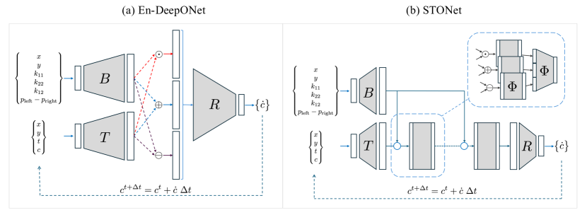
3.2 STONet
Here, we present an extension of the En-DeepONet architecture that resembles the multi-head attention mechanism of transformer networks [31]. The network architecture is depicted in fig. 1(b). The architecture consists of an encoding branch and a trunk network. The output of the branch network is then combined with the output of the trunk network, using elementwise operations such as multiplication or addition, and passed to the new attention block. One may add multiple attention blocks. The final output is then passed on to the output root network. The network architecture is expressed mathematically as
| (12) | ||||
| (13) | ||||
| (14) | ||||
| (15) | ||||
| (16) | ||||
| (17) | ||||
| (18) | ||||
| (19) |
where denotes a single fully-connected layer, and is the total number of attention blocks. Lastly, the network is trained on the concentration rate, therefore concentration field is predicted auto-regressively using the forward Euler update as
| (20) |
3.3 Optimization
The optimization of neural operators involves adjusting the parameters of the branch, trunk, and root networks to minimize a loss function that measures the discrepancy between the predicted and true outputs. In this study, the network output is the concentration rate , as mentioned previously. Hence, the loss function is based on the mean squared error between the predicted and observed solute concentrations. The optimization is performed using the Adam optimizer [18], a variant of the stochastic gradient descent. The gradients are computed using backpropagation through the computational graph of the neural operator. Regularization techniques, such as weight decay or dropout, may be employed to prevent overfitting and improve the generalization of the model.
4. Results and Discussion
In this section, we present the results of our numerical experiments on the performance of the proposed neural operator for surrogate modeling of solute transport in micro-cracked reservoirs. We compare the accuracy and computational efficiency of our approach to the finite element method. Additionally, we evaluate the effectiveness of the neural operator in handling different input scenarios and encoding heterogeneous properties of the porous medium. Finally, we discuss the potential applications of our model in environmental impact assessment and groundwater management.
4.1 Problem Description
A schematic of the problem considered in this study of a solute through a micro-cracked reservoir is shown in fig. 2. The domain under consideration has dimensions of cm. The solution is injected from the left side and transported through the domain, driven by a pressure difference between the left and right boundaries. The porous reservoir is assumed to be confined between two impervious layers and contains randomly distributed micro-cracks of varying density and orientations. The micro-fracture orientations are sampled randomly from a normal distribution with varying mean values but fixed standard deviation, i.e., , where is sampled uniformly as . The representative elementary volume (REV) dimensions for assessing the permeability field (using eq. (5)) are assumed cm. Fracture density, i.e., the number of cracks per REV, is sampled from a Poisson’s distribution as , where is sampled uniformly as . Fracture length and aperture are sampled from log-normal distributions and , respectively. The pressure on the left side is kept fixed, while the pressure on the right side is also randomly perturbed from a normal distribution, i.e., . fig. 3 depicts a sample medium with micro-fractures.
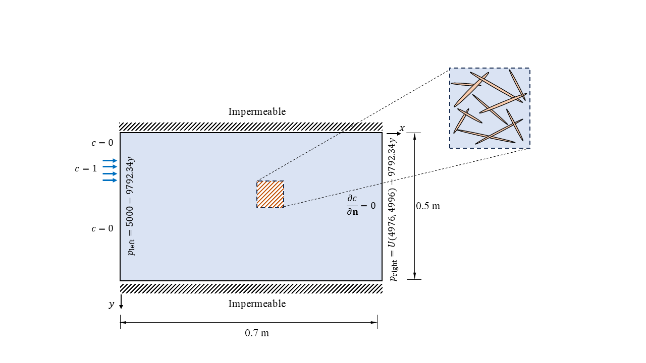
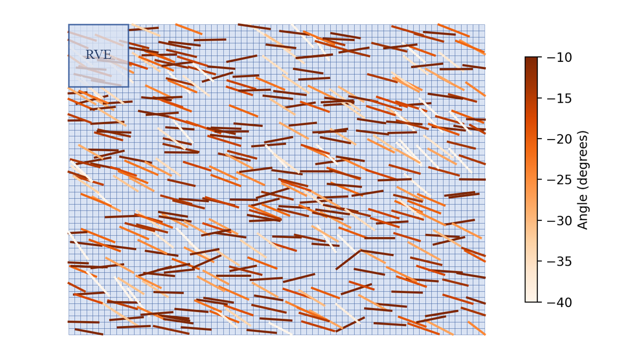
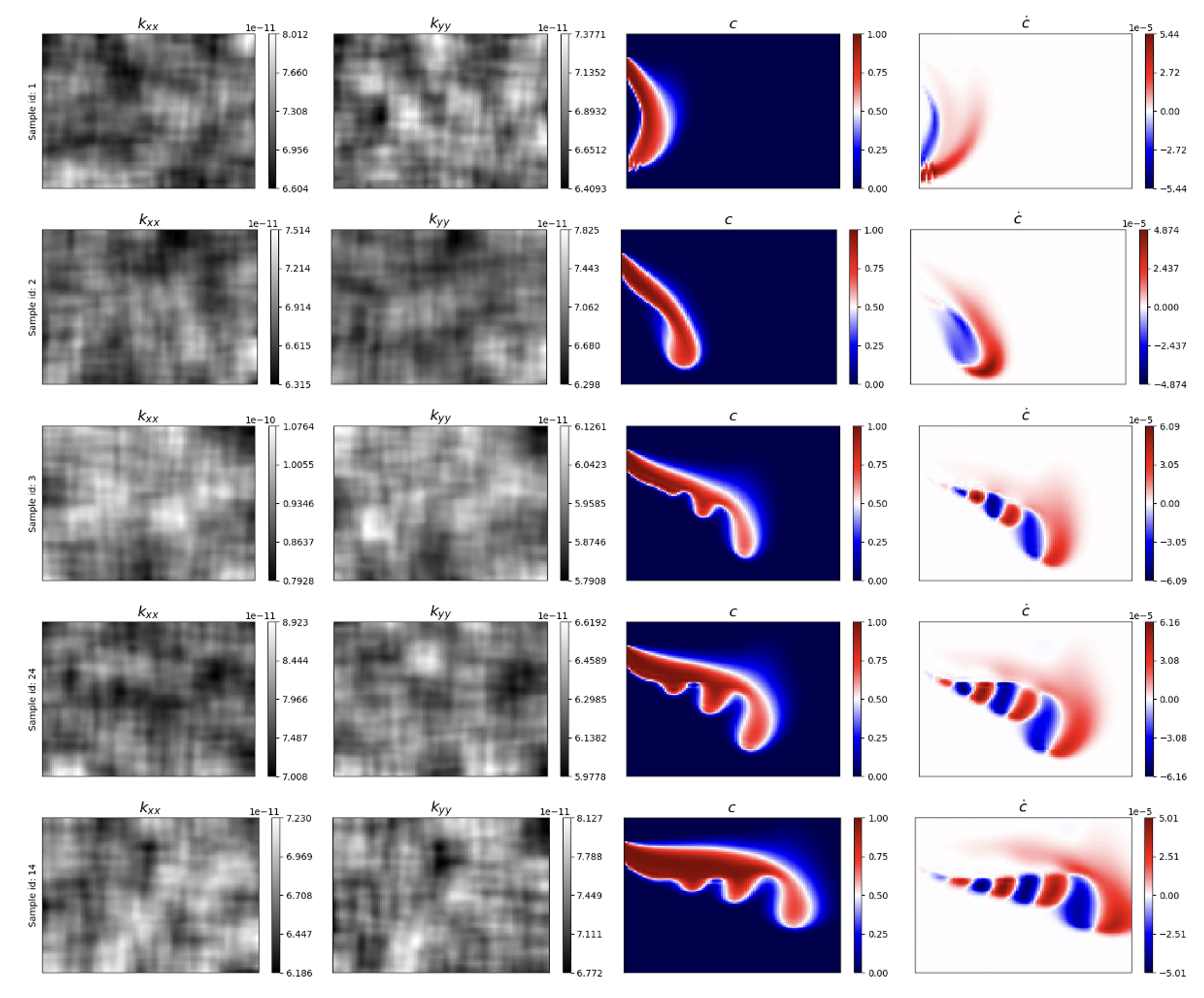
Figure 4 depicts a few snapshots of the solute concentration for different micro-crack distributions. The equivalent permeability field () and () are plotted in the left two columns, while the right two columns highlight concentration and the rate of change of concentration at the last time step (i.e., hr). The changes in the concentration patterns are due to different fracture orientations and pressure gradients.
The training dataset consists of 500 FEM simulations, and the test dataset consists of 25 random unseen samples. The domain is discretized using an element dimension of cm, resulting in a total of 3,500 elements and 3,621 nodes. We run the simulation for a total of h using s implicit time increments. However, the outputs are recorded only at h time increments. The generated dataset covers a wide range of fracture densities, orientations, and lengths, providing a diverse set of training examples for our neural operator.
4.2 Sampling Strategy
Since concentration remains near zero for a large portion of the domain (as shown in fig. 4), to reduce the batch size and computational demand, we sub-sample 1,500 random nodes using an importance sampling strategy. Out of these, 1,000 points were selected based on concentration density, while the remaining 500 nodes were uniformly distributed over the domain.
4.3 Training Performance
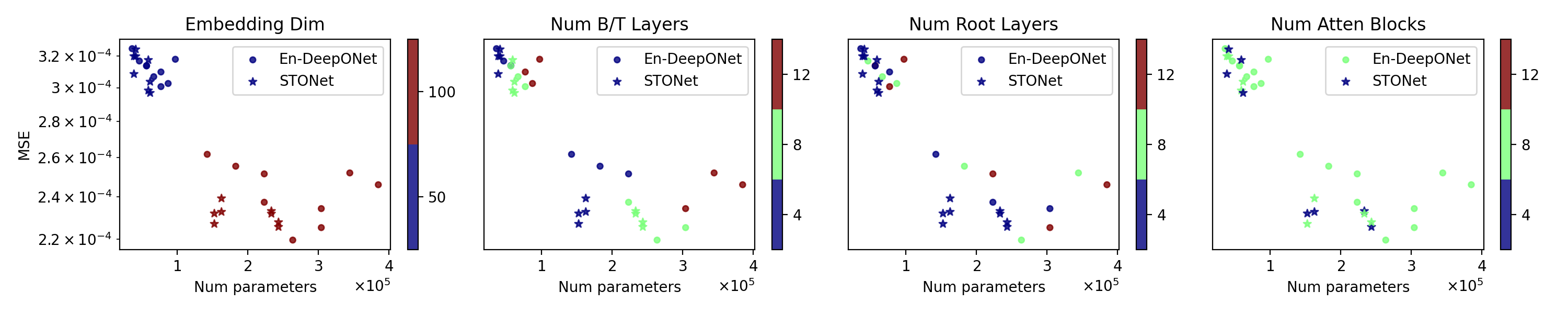
Let us first compare the performance of the new En-DeepONet architecture (i.e., STONet) with respect to the original architecture. To this end, we vary the network width and embedding dimensions in , the number of layers of the branch and trunk networks in , and the number of the layers of the root network in and number of attention blocks in . The results are shown in fig. 5, where circles indicate the loss with the traditional En-DeepONet architecture, and the star symbols the loss with the new STONet architecture. We observe that for a similar number of parameters, the new STONet architecture outperforms the previous architecture without an increase in the computational cost. We also observe that both architectures improve their performance for larger network widths.
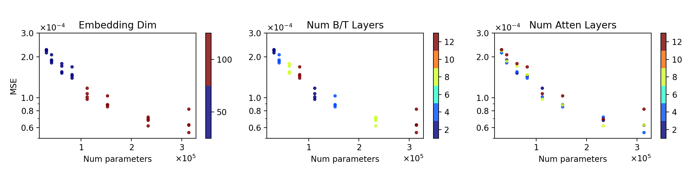
Next, to arrive at the optimal neural architecture for modeling this dataset, we explored several network sizes. The first variable is the network width of all networks (i.e., B, T, R, ) along with their output dimension (embedding) from . The second variable is the number of layers in the branch and trunk networks from . The third variable is the number of attention blocks from . The training is performed for 2,000 epochs, and the average loss for the last 100 epochs is compared.
The results of hyper-parameter exploration are shown in fig. 6. The horizontal axis shows the total number of parameters, while the vertical axis presents the average of the loss value for the last 100 epochs. It is apparent that wider networks lead to a significant improvement in performance. The optimal choice of parameters seems to be 100 for network width, 8 layers for the branch and trunk networks, 8 attention blocks, and 2 root layers. Therefore, this architecture is utilized with further training (up to 50,000 epochs) to arrive at the results presented in the next section.
4.4 Model Performance
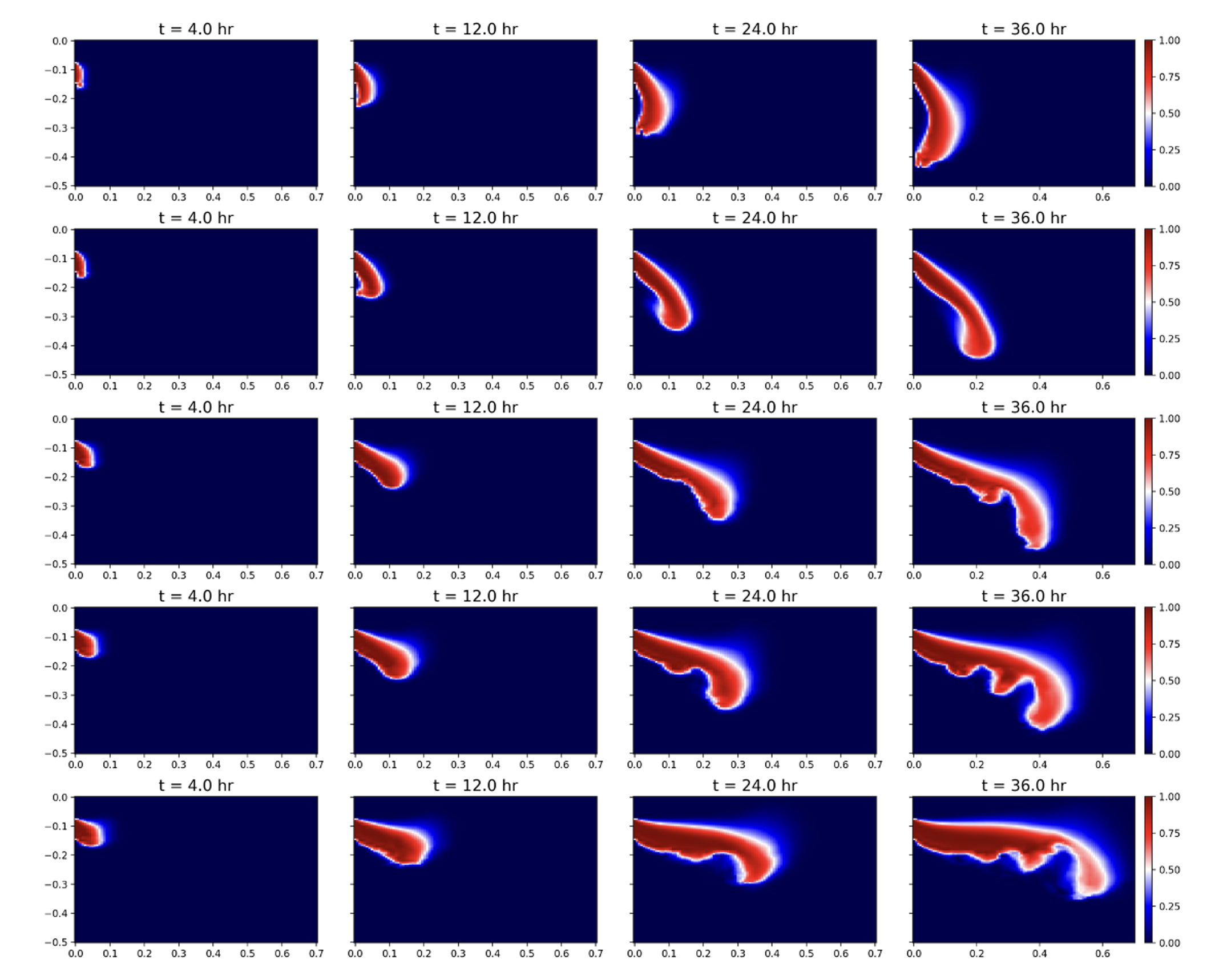
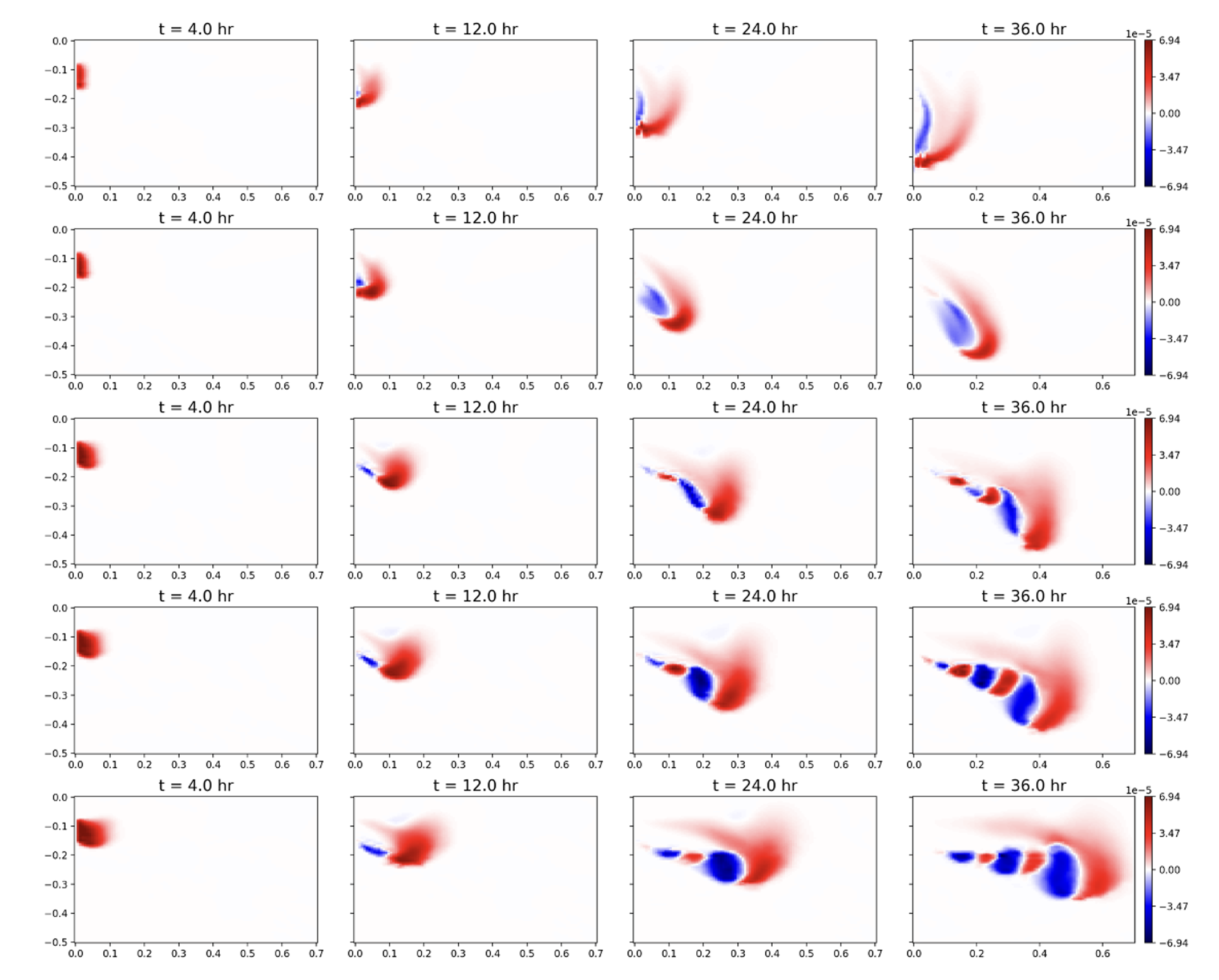
Figure 7 depicts the predictions for the concentration on five random realizations from the test set. The corresponding predictions for the rate of change of concentration are shown in fig. 8. The results from the full-physics simulations for these five test cases were shown earlier in fig. 4. It is apparent that STONet predicts the full-physics results accurately. The fundamental difference is that the STONet, having been pre-trained, can be used for fast prediction of density-driven flow and transport with any new fracture network, while the FEM simulation would need to be recomputed altogether for any new configuration.
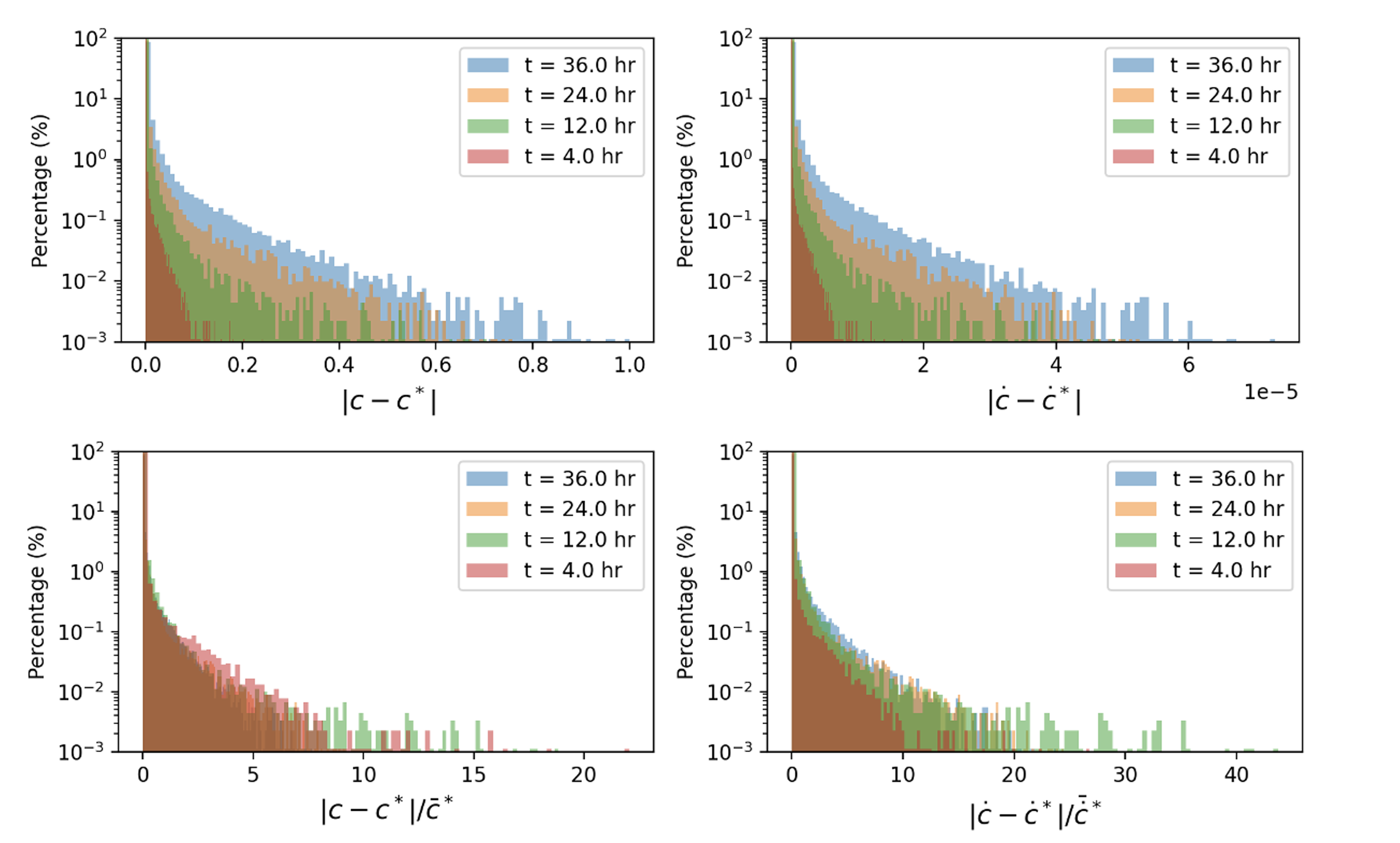
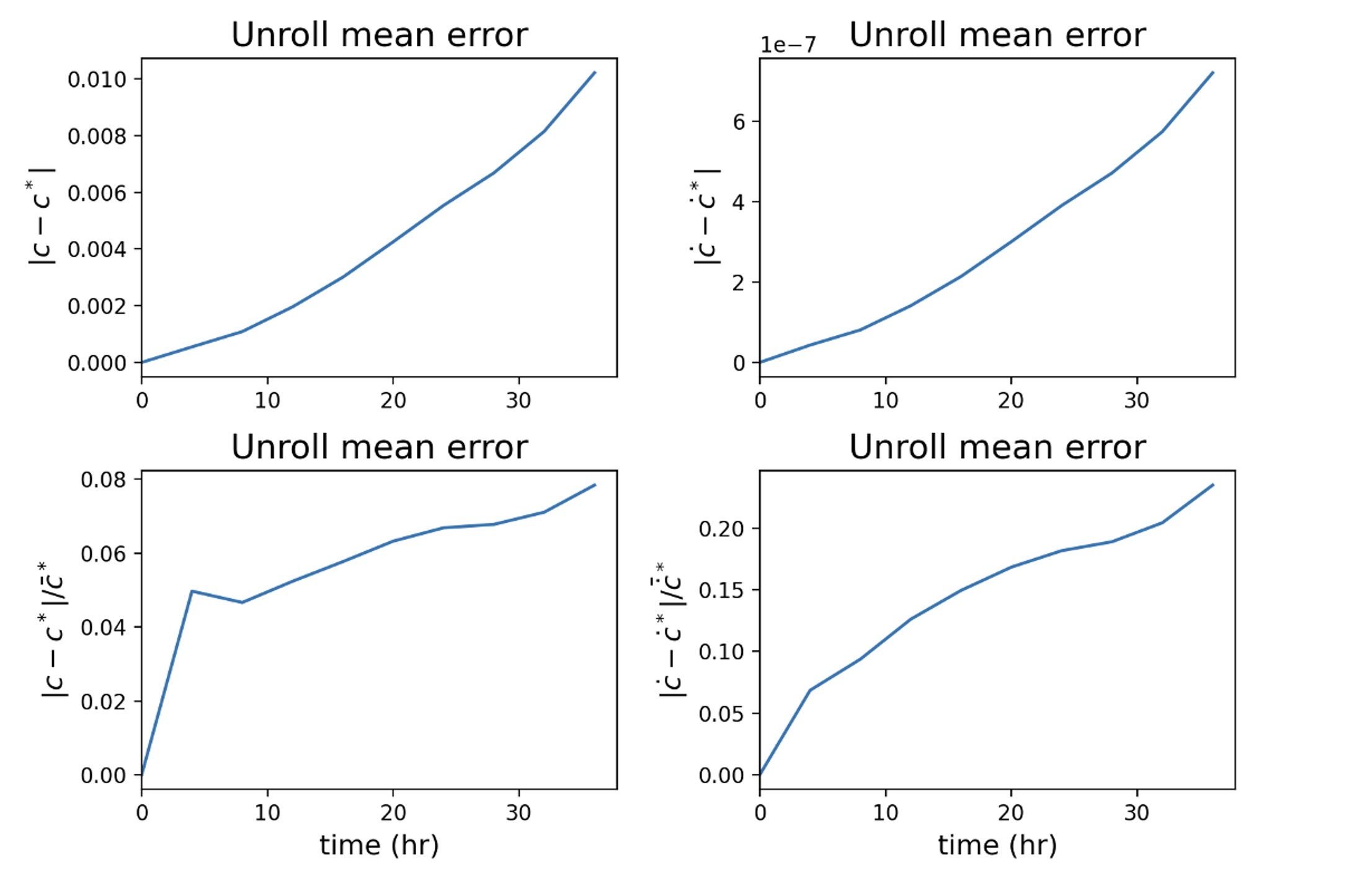
The distributions for pointwise absolute and relative error at different time steps for concentration and concentration rate are plotted in Figure 9. Overall, STONet’s prediction error is very small, with most predictions having below 1% error. The top figures depict the absolute error distributions and highlight the presence of accumulation error as can be observed from widening distributions at different time steps. However, the distribution of relative error at different time steps, as shown in the bottom figures, remains nearly unchanged, indicating a predictable fixed error distribution over time, which is highly desirable. This is also confirmed by inspecting the mean absolute and relative error evolution over time, as plotted in fig. 10. It is worth noting that the accumulation error might be controlled with the addition of observational data and additional training samples using data assimilation techniques such as Active Learning [32].
5. Conclusions
In this study, we have presented a new Enriched-DeepONet architecture, STONet, for emulating density-driven flow and solute transport in micro-cracked reservoirs. Our approach effectively encodes heterogeneous properties and predicts the concentration rate, achieving accuracy comparable to that of the finite element method. The computational efficiency of STONet enables rapid and accurate predictions of solute transport, facilitating both parameter identification and groundwater management optimization.
The STONet model developed in this work has the potential to be applied for fracture network identification and efficient tracing and control of solute transport in micro-cracked reservoirs. By rapidly and accurately predicting the concentration rate, the model can help identify the location and connectivity of fractures in the porous media, which is crucial for optimizing the management of groundwater resources. Additionally, the model can be used to predict the transport of solutes in different scenarios, such as accidental contaminant spills, allowing for accurate and efficient decision-making. Overall, the ML model has the potential to significantly improve the sustainable management of underground aquifers, contributing to both local and global efforts towards sustainable groundwater resource utilization.
Conflicts of Interest
The authors have no conflicts of interest to declare.
Author Contributions
EH conceptualized the problem and contributed to the theoretical development and implementation. MHA contributed to the implementation, running the test cases and generating the figures. MM prepared the training dataset. All authors contributed to drafting and revising the manuscript.
Data availability
The data and code for reproducing the results reported in this manuscript will be published at https://github.com/ehsanhaghighat/STONet.
References
- Abarca et al. [2006] E. Abarca, E. Vázquez-Suñé, J. Carrera, B. Capino, D. Gámez, and F. Batlle. Optimal design of measures to correct seawater intrusion. Water Resources Research, 42(9):W09415, 2006.
- Amini et al. [2022] D. Amini, E. Haghighat, and R. Juanes. Physics-informed neural network solution of thermo–hydro–mechanical processes in porous media. Journal of Engineering Mechanics, 148(11):04022070, 2022.
- Cai et al. [2021] S. Cai, Z. Mao, Z. Wang, M. Yin, and G. E. Karniadakis. Physics-informed neural networks (pinns) for fluid mechanics: A review. Acta Mechanica Sinica, 37(12):1727–1738, 2021.
- Cuomo et al. [2022] S. Cuomo, V. S. Di Cola, F. Giampaolo, G. Rozza, M. Raissi, and F. Piccialli. Scientific machine learning through physics–informed neural networks: Where we are and what’s next. Journal of Scientific Computing, 92(3):88, 2022.
- Dentz et al. [2006] M. Dentz, D. Tartakovsky, E. Abarca, A. Guadagnini, X. Sanchez-Vila, and J. Carrera. Variable-density flow in porous media. Journal of fluid mechanics, 561:209–235, 2006.
- Diersch and Kolditz [2002] H.-J. Diersch and O. Kolditz. Variable-density flow and transport in porous media: approaches and challenges. Advances in water resources, 25(8-12):899–944, 2002.
- Diersch [2013] H.-J. G. Diersch. FEFLOW: finite element modeling of flow, mass and heat transport in porous and fractured media. Springer Science & Business Media, 2013.
- Faulkner et al. [2010] D. Faulkner, C. Jackson, R. Lunn, R. Schlische, Z. Shipton, C. Wibberley, and M. Withjack. A review of recent developments concerning the structure, mechanics and fluid flow properties of fault zones. Journal of Structural Geology, 32(11):1557–1575, 2010.
- Haghighat et al. [2021] E. Haghighat, M. Raissi, A. Moure, H. Gomez, and R. Juanes. A physics-informed deep learning framework for inversion and surrogate modeling in solid mechanics. Computer Methods in Applied Mechanics and Engineering, 379:113741, 2021.
- Haghighat et al. [2022] E. Haghighat, D. Amini, and R. Juanes. Physics-informed neural network simulation of multiphase poroelasticity using stress-split sequential training. Computer Methods in Applied Mechanics and Engineering, 397:115141, 2022.
- Haghighat et al. [2024] E. Haghighat, U. bin Waheed, and G. Karniadakis. En-deeponet: An enrichment approach for enhancing the expressivity of neural operators with applications to seismology. Computer Methods in Applied Mechanics and Engineering, 420:116681, 2024.
- Juanes et al. [2002] R. Juanes, J. Samper, and J. Molinero. A general and efficient formulation of fractures and boundary conditions in the finite element method. International Journal for Numerical Methods in Engineering, 54(12):1751–1774, 2002.
- Karniadakis et al. [2021] G. E. Karniadakis, I. G. Kevrekidis, L. Lu, P. Perdikaris, S. Wang, and L. Yang. Physics-informed machine learning. Nature Reviews Physics, 3(6):422–440, 2021.
- Khoei et al. [2016] A. Khoei, N. Hosseini, and T. Mohammadnejad. Numerical modeling of two-phase fluid flow in deformable fractured porous media using the extended finite element method and an equivalent continuum model. Advances in water resources, 94:510–528, 2016.
- Khoei et al. [2023a] A. Khoei, S. Mousavi, and N. Hosseini. Modeling density-driven flow and solute transport in heterogeneous reservoirs with micro/macro fractures. Advances in Water Resources, 182:104571, 2023a.
- Khoei et al. [2023b] A. Khoei, S. Saeedmonir, N. Hosseini, and S. Mousavi. An x–fem technique for numerical simulation of variable-density flow in fractured porous media. MethodsX, 10:102137, 2023b.
- Khoei and Taghvaei [2024] A. R. Khoei and M. Taghvaei. A computational dual-porosity approach for the coupled hydro-mechanical analysis of fractured porous media. International Journal for Numerical and Analytical Methods in Geomechanics, 2024.
- Kingma [2014] D. P. Kingma. Adam: A method for stochastic optimization. arXiv preprint arXiv:1412.6980, 2014.
- Kovachki et al. [2023] N. Kovachki, Z. Li, B. Liu, K. Azizzadenesheli, K. Bhattacharya, A. Stuart, and A. Anandkumar. Neural operator: Learning maps between function spaces with applications to pdes. Journal of Machine Learning Research, 24(89):1–97, 2023.
- LeCun et al. [2015] Y. LeCun, Y. Bengio, and G. Hinton. Deep learning. nature, 521(7553):436–444, 2015.
- Li et al. [2020] Z. Li, N. Kovachki, K. Azizzadenesheli, B. Liu, K. Bhattacharya, A. Stuart, and A. Anandkumar. Neural operator: Graph kernel network for partial differential equations. arXiv preprint arXiv:2003.03485, 2020.
- Lu et al. [2021] L. Lu, P. Jin, G. Pang, Z. Zhang, and G. E. Karniadakis. Learning nonlinear operators via deeponet based on the universal approximation theorem of operators. Nature machine intelligence, 3(3):218–229, 2021.
- Molinero et al. [2002] J. Molinero, J. Samper, and R. Juanes. Numerical modeling of the transient hydrogeological response produced by tunnel construction in fractured bedrocks. Engineering Geology, 64(4):369–386, 2002.
- Musuuza et al. [2009] J. L. Musuuza, S. Attinger, and F. A. Radu. An extended stability criterion for density-driven flows in homogeneous porous media. Advances in water resources, 32(6):796–808, 2009.
- Niaki et al. [2021] S. A. Niaki, E. Haghighat, T. Campbell, A. Poursartip, and R. Vaziri. Physics-informed neural network for modelling the thermochemical curing process of composite-tool systems during manufacture. Computer Methods in Applied Mechanics and Engineering, 384:113959, 2021.
- Oda [1986] M. Oda. An equivalent continuum model for coupled stress and fluid flow analysis in jointed rock masses. Water resources research, 22(13):1845–1856, 1986.
- Raissi et al. [2019] M. Raissi, P. Perdikaris, and G. E. Karniadakis. Physics-informed neural networks: A deep learning framework for solving forward and inverse problems involving nonlinear partial differential equations. Journal of Computational physics, 378:686–707, 2019.
- Saeedmonir et al. [2024] S. Saeedmonir, M. Adeli, and A. Khoei. A multiscale approach in modeling of chemically reactive porous media. Computers and Geotechnics, 165:105818, 2024.
- Schincariol et al. [1997] R. A. Schincariol, F. W. Schwartz, and C. A. Mendoza. Instabilities in variable density flows: Stability and sensitivity analyses for homogeneous and heterogeneous media. Water resources research, 33(1):31–41, 1997.
- Sebben et al. [2015] M. L. Sebben, A. D. Werner, and T. Graf. Seawater intrusion in fractured coastal aquifers: A preliminary numerical investigation using a fractured henry problem. Advances in water resources, 85:93–108, 2015.
- Vaswani [2017] A. Vaswani. Attention is all you need. Advances in Neural Information Processing Systems, 2017.
- Wang et al. [2023] N. Wang, H. Chang, and D. Zhang. Inverse modeling for subsurface flow based on deep learning surrogates and active learning strategies. Water Resources Research, 59(7):e2022WR033644, 2023.
- Wang et al. [2021] S. Wang, H. Wang, and P. Perdikaris. Learning the solution operator of parametric partial differential equations with physics-informed deeponets. Science advances, 7(40):eabi8605, 2021.
- Wen et al. [2022] G. Wen, Z. Li, K. Azizzadenesheli, A. Anandkumar, and S. M. Benson. U-fno—an enhanced fourier neural operator-based deep-learning model for multiphase flow. Advances in Water Resources, 163:104180, 2022.
- Zeytounian [2003] R. K. Zeytounian. Joseph boussinesq and his approximation: a contemporary view. Comptes Rendus Mecanique, 331(8):575–586, 2003.
- Zhou et al. [2008] C. B. Zhou, R. S. Sharma, Y. F. Chen, and G. Rong. Flow–stress coupled permeability tensor for fractured rock masses. International Journal for Numerical and Analytical Methods in Geomechanics, 32(11):1289–1309, 2008.