Rydberg Atomic Quantum Receivers for
Classical Wireless Communications and Sensing:
Their Models and Performance

Abstract

The significant progress of quantum sensing technologies offer numerous radical solutions for measuring a multitude of physical quantities at an unprecedented precision. Among them, Rydberg atomic quantum receivers (RAQRs) emerge as an eminent solution for detecting the electric field of radio frequency (RF) signals, exhibiting a great potential in assisting classical wireless communications and sensing. So far, most experimental studies have aimed for the proof of physical concepts to reveal its promise, while the practical signal model of RAQR-aided wireless communications and sensing remained under-explored. Furthermore, the performance of RAQR-based wireless receivers and their advantages over the conventional RF receivers have not been fully characterized. To fill the gap, we introduce the superheterodyne version of RAQRs to the wireless community by presenting an end-to-end reception scheme. We then develop a corresponding equivalent baseband signal model relying on a realistic reception flow. Our scheme and model provide explicit design guidance to RAQR-aided wireless systems. We next study the performance of RAQR-aided wireless systems based on our model, and compare them to a half-wavelength dipole antenna based conventional RF receiver. The results show that the RAQR is capable of achieving a substantial receive signal-to-noise ratio (SNR) gain of $\sim 22.6$ decibel (dB) and $\sim 33.5$ dB in the standard (unoptimized) and optimized configurations, respectively.

I Introduction

The growing thirst for high data rate, large-scale connectivity, and ultra-reliable low latency are the distinctive features of the next-generation (NG) wireless systems, in which a multitude of upper-layer applications and a wide variety of functionalities over a large spatial distribution are expected to be supported [1]. To support these visions, developing advanced high-sensitivity receivers and exploiting a wide range of untapped spectral resources becomes paramount. Both require the radio-frequency (RF) receivers capable of detecting RF signals with extremely low strength and broadband spectrum. To realize these visions, the conventional technology road-map relies on the advances of integrated circuits (ICs) and antenna technologies.

State-of-the-art RF receivers rely on well-calibrated antennas, filters, amplifiers, and mixers [2]. The sensitivity of IC-based receivers is typically limited by the extrinsic noise background, the bandwidth, the noise figure of ICs, and the signal-to-noise ratio (SNR) required for demodulation. Therefore, designing high-quality ICs becomes an effective technique of increasing the sensitivity of RF receivers. Furthermore, strong reception capability may be achieved by harnessing multiple antennas, where multiple copies of an RF signal can be obtained for suppressing noise contamination and/or wireless channel fading. The emergence of multiple-input multiple-output (MIMO) systems relies on sophisticated multiple-antenna technology. Their concept has evolved from the massive MIMO philosophy [3] to the development of holographic MIMO [4, 5]. For broadband signal reception and processing, the RF receivers may be implemented by relying on multiple IC channels, where each channel is responsible for a specific frequency band. Such a naive IC stacking scheme is bulky, power-thirsty, and heavily relies on advanced IC manufacturing technologies, suffering from many design challenges, particularly when designing complex high-frequency receivers.

The ‘second quantum revolution’ [6] rests on three main pillars of quantum technologies, which are quantum computing, quantum communications, and quantum sensing. Specifically, quantum sensing includes but it is not limited to quantum precision measurements and quantum metrology, which rely on the use of quantum phenomena to perform a measurement of a physical quantity [7]. The physical quantity is associated with the intrinsic properties of microscopic particles that are capable of facilitating an unprecedented level of sensitivity. Based on this, a multitude of quantum sensing applications have emerged for measuring a wide variety of physical quantities, such as electric fields, magnetic fields, frequency, temperature, pressure, rotation, acceleration, and so forth [8]. Among the various quantum sensing technologies, those relying on Rydberg atoms exhibit an exceptional sensitivity in detecting electric fields [9, 10, 11], paving the way for realizing Rydberg atomic quantum receiver (RAQR) aided wireless communications and sensing [12]. Additionally, the ambition of using quantum-domain solutions for enhancing the performance of classical wireless systems was documented for example in [13, 14].

Apart from their extremely high sensitivity, RAQRs have numerous compelling advantages, such as broadband tunability, compact form factor, and International System of Units (SI)-traceability [11, 12]. Hence they offer a radical solution to those RF reception challenges. Firstly, the high sensitivity of RAQRs is a direct benefit of the highly-excited state of Rydberg atoms, where their outermost electrons are excited to a very high energy level. The highly-excited states exhibit a remarkably large dipole moment that is extremely sensitive to the external coupling of RF signals. The high sensitivity of RAQRs has been experimentally shown to be on the order of µV/cm/$\sqrt{\text{Hz}}$ using a standard structure [15, 16, 11]. This has also been improved to $55$ nV/cm/$\sqrt{\text{Hz}}$ using a superheterodyne structure [17, 18], and can be further enhanced via repumping [19]. Another recent work further enhanced the sensitivity to $3.98$ nV/cm/$\sqrt{\text{Hz}}$ [20]. The sensitivity limit of RAQRs may even reach pV/cm/$\sqrt{\text{Hz}}$ obeying the standard quantum limit (SQL). Secondly, RAQRs are capable of receiving RF frequencies spanning from near direct-current to Terahertz (THz) frequencies using a single vapor cell, exhibiting broadband tunability. One or more of the RF signals to be processed may be at different but specific discrete frequencies [21, 22, 23], or at any frequency of a specific continuous range [24, 25, 26]. Thirdly, RAQRs can directly down-convert RF signals to baseband without using any complex processing, hence significantly simplifying the receiver’s structure compared to that of the conventional RF receiver. More particularly, the size of RAQRs is independent of the wavelength of RF signals. Furthermore, RAQRs are capable of acquiring precise measurements directly linked to SI without any calibration. Finally, RAQRs are omnidirectional, capable of receiving RF signals from all angular directions.

The above-mentioned prominent features and powerful capabilities of RAQRs make them appealing in assisting classical wireless communications and sensing. However, the current studies are essentially limited to an experimental perspective from the physics community. They focused on improving the sensitivity [18, 19, 20], and on developing multi-band [21, 22, 23] or continuous-band detection [24, 25, 26]. They also realize various functionalities, such as detection of amplitude [15, 16, 11], phase [17, 18, 19], polarization [27, 28, 29], modulation [30, 31, 32], spatial direction [33], and spatial displacement [34]. Furthermore, several initial applications verifying the benefits of RAQRs in assisting communications were experimentally presented in [35, 36, 37, 38]. The above experimental studies have demonstrated the feasibility of RAQRs, but they fail to support theoretical studies due to the lack of a complete end-to-end signal model. There are also a pair of emerging studies [39, 40] from the communication society, which introduce RAQRs to MIMO communications from a signal processing perspective. These mainly emphasize their algorithmic designs based on a system model abstracted from a two-level quantum system. However, this model may be simple and inaccurate in describing a realistic RAQR that is typically a four-level quantum system. Moreover, a comprehensive overview of RAQRs designed for classical wireless communications and sensing was presented in [12]. In summary, the study of RAQRs for classical wireless communications and sensing is in its infancy. Clearly, a practical signal model, bridging physics and communications/sensing, is urgently needed for system design and signal processing.

To fill this knowledge gap and unlock the full potential of RAQRs in classical wireless communications and sensing, we study the superheterodyne RAQR as a benefit of its high sensitivity and capability in both amplitude and phase detection. Explicitly, we offer the following contributions.

• We study the typical four-level quantum scheme in depicting the realistic superheterodyne RAQRs, and derive a closed-form expression of the density coefficient related to the so-called $\ket{1}$→$\ket{2}$ transition under realistic assumptions. We associate the probe beam with this density coefficient for characterizing its amplitude and phase. The expression derived offers a precise evaluation on the transformation (transfer function of RAQRs) from the input RF signal to the output probe beam. It also paves the way for jointly optimizing diverse parameters of RAQRs, e.g., the frequency detuning and power of laser beams and the local oscillator (LO).

• We construct an end-to-end RAQR-aided wireless reception scheme by detailing each of the functional blocks and derive the corresponding input-output equivalent baseband signal model of the overall system. The scheme follows a realistic signal reception flow of an RAQR, offering explicit design guidance for RAQR-aided wireless systems. The proposed signal model reveals that the RAQR imposes a gain and phase shift on the baseband transmit signal, where these factors are determined by both the atomic response and the specific photodetection scheme. The form of our signal model is consistent with that of the conventional RF receiver, paving the way for performing various signal processing tasks.

• We further investigate the noise sources that contaminate an RAQR, where both extrinsic and intrinsic noises are considered. The former includes the black-body radiation induced thermal noise [41], while the latter encompasses the photodetector’s shot noise (PSN) [42, Ch. 5], the intrinsic thermal noise (ITN) [43, Ch. 16], and the quantum projection noise (QPN) [44, 16, 45]. The PSN may dominate among all noise sources, and the QPN can be reasonably neglected by increasing the number of Rydberg atoms in the vapor cell.

• We next study the performance of RAQR-aided wireless systems, where we present the receive SNR of the system for two different photodetection schemes, namely the direct incoherent optical detection and the balanced coherent optical detection. We theoretically demonstrate that the latter scheme outperforms the former scheme in terms of the receive SNR. Their SNR ratio is derived for the PSN-dominated case. Furthermore, we compare the RAQRs to the conventional RF receivers, where we derive the lower bound condition of the RAQR gain to guarantee its superiority over its conventional counterparts. Particularly, the RAQRs having a modest setup is capable of outperforming a half-wavelength dipole antenna based RF receiver in terms of the receive SNR, offering an extra SNR gain of $\sim 22.6$ dB and $\sim 33.5$ dB in the standard (unoptimized) and optimized configurations, respectively.

• We finally perform diverse numerical simulations to validate the proposed signal model and characterize the performance of the RAQRs. Our results verify their effectiveness and demonstrate the superiority of RAQRs in assisting classical wireless communications and sensing.

Organization and Notations: The article is organized as follows. In Section II, we construct the quantum response model of the superheterodyne RAQRs. In Section III, we propose an RAQR-aided wireless reception scheme and detail the corresponding equivalent baseband signal model. In Section IV, we analyse the performance of RAQRs. We then proceed by presenting our simulation results in Section V, and finally conclude the article in Section VI. The notations $\frac{\mathrm{d}\bm{\rho}}{\mathrm{d}t}$ represent the differential of $\bm{\rho}$ with respect to time; $\commutator{\bm{H}}{\bm{\rho}}=\bm{H}\bm{\rho}-\bm{\rho}\bm{H}$ represents the commutator; $\left\{\bm{\varGamma},\bm{\rho}\right\}=\bm{\varGamma}\bm{\rho}+\bm{\rho}\bm{\varGamma}$ stands for the anticommutator; $\mathscr{R}\{\cdot\}$ and $\mathscr{I}\{\cdot\}$ take the real and imaginary parts of a complex number; $\text{diag}\{\cdot\}$ denotes the diagonal of a matrix; $\chi^{\prime}$ represents the derivative of $\chi$; $\hbar$ is the reduced Planck constant and $\jmath^{2}=1$; $c$ is the speed of light in free space and $\epsilon_{0}$ is the vacuum permittivity; $\eta$ is the quantum efficiency of the photodetector and $q$ is the elementary charge.

II The Quantum Response Model of RAQR

We adopt the superheterodyne structure of RAQRs [18] in our receiver, as a benefit of its high sensitivity and powerful capability of receiving various modulated RF signals, which will not be detailed hereafter. The architecture of RAQR is portrayed in Fig 1(a). Briefly, it consists of a vapor cell containing alkali atoms (Cesium (Cs) or Rubidium (Rb) atoms), and a pair of laser beams (probe and coupling). The laser beams counter-propagate through the vapor cell to form a spatially overlapped receive area, in which Rydberg atoms are prepared. A local RF source having a resonant frequency identical to the transition frequency between the Rydberg states employed serves as the LO. The superposition of the desired RF signal and LO alters the atomic response, which is optically read-out and subsequently detected by a photodetector. The RAQR serves as an RF to optical converter, which is facilitated by utilizing the EIT phenomenon [9, 10, 11, 12].

II-A The Electron Transition Model of RAQR

The electron transitions happening in the receive area of the vapor cell may be described by a four-level ladder scheme, as shown in Fig. 1(b). The electron transition between the ground state $\ket{1}$ and the excited state $\ket{2}$ is (near-) resonantly coupled with the probe beam having a Rabi frequency [11] of $\Omega_{p}$ and angular frequency of $\omega_{p}$. This excited state is further driven by the coupling beam of Rabi frequency $\Omega_{c}$ and of angular frequency $\omega_{c}$. The LO of Rabi frequency $\Omega_{l}$ and of angular frequency $\omega_{l}$ further (near-) resonantly excites the transition between the so-called Rydberg states $\ket{3}$ and $\ket{4}$. The probe, coupling and LO fields may be detuned (have a frequency difference) around their corresponding resonant frequencies. The detuning frequencies (frequency differences) corresponding to the probe beam, the coupling beam, and the LO are $\Delta_{p}=\omega_{12}-\omega_{p}$, $\Delta_{c}=\omega_{23}-\omega_{c}$, and $\Delta_{l}=\omega_{34}-\omega_{l}$, respectively, where $\omega_{i-1,i}$ is the resonant angular frequency between level $\ket{i-1}$ and $\ket{i}$, $i=2,3,4$. $\gamma_{i}$ is the spontaneous decay rate of the $i$-th level. To elaborate a little further, $\gamma$ and $\gamma_{c}$ are the relaxation rates related to the atomic transition effect and the atomic collision effect, respectively. For simplicity, we assume $\gamma=\gamma_{c}=0$. Additionally, we assume that the decay rates of level $\ket{3}$ and level $\ket{4}$ are comparatively low so that they can be reasonably ignored. The impinging RF signal to be detected produces a coupling $\Omega_{x}\cos{(2\pi f_{\delta}t+\theta_{\delta})}$, which has a frequency offset of $f_{\delta}$ and a phase offset of $\theta_{\delta}$ relative to the LO. Furthermore, the RAQR requires $\Omega_{x}\ll\Omega_{l}$, implying that the impinging RF is weak compared to the LO [18].

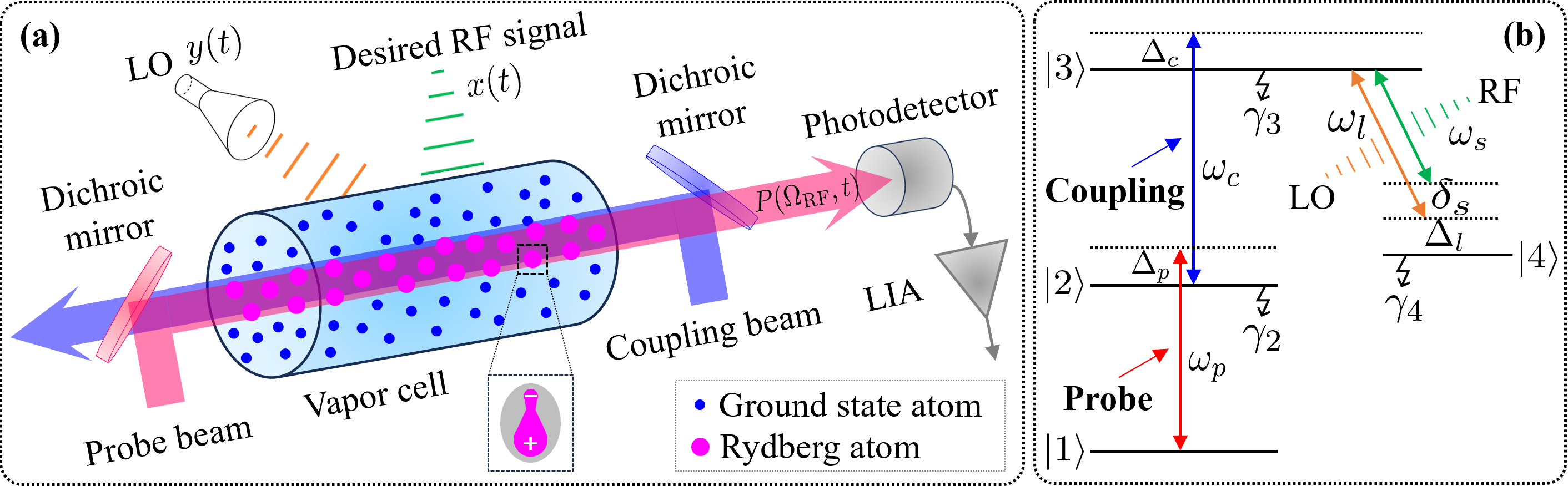
Figure 1: (a) The superheterodyne structure of RAQRs, and (b) its corresponding four-level scheme.

To elaborate a little further, typically, the Lindblad master equation is applied for characterizing the dynamics of the four-level transition scheme, which is given by [46, Ch. 10]

$$\frac{\mathrm{d}\bm{\rho}}{\mathrm{d}t}=-\jmath\commutator{\bm{H}}{\bm{\rho}}-\frac{1}{2}\left\{\bm{\varGamma},\bm{\rho}\right\}+\bm{\varLambda},$$ (1)

where $\bm{H}$, $\bm{\varGamma}$ and $\bm{\varLambda}$ are the Hamiltonian, the relaxation matrix, and the decay matrix, respectively. They are given by [46]

$$\bm{H} =\left[{\begin{array}[]{*{20}{c}}0&{\frac{{{\Omega_{p}}}}{2}}&0&0\\ {\frac{{{\Omega_{p}}}}{2}}&{{\Delta_{p}}}&{\frac{{{\Omega_{c}}}}{2}}&0\\ 0&{\frac{{{\Omega_{c}}}}{2}}&{{\Delta_{p}}+{\Delta_{c}}}&{\frac{{{\Omega_{\text{RF}}}}}{2}}\\ 0&0&{\frac{{{\Omega_{\text{RF}}}}}{2}}&{{\Delta_{p}}+{\Delta_{c}}+{\Delta_{l}}}\end{array}}\right],$$ (6)

$\bm{\varGamma}=\text{diag}\{\gamma,\gamma+\gamma_{2},\gamma+\gamma_{3}+\gamma_{c},\gamma+\gamma_{4}\}$, and $\bm{\varLambda}=\text{diag}\{\gamma+\gamma_{2}\rho_{22}+\gamma_{4}\rho_{44},\gamma_{3}\rho_{33},0,0\}$. In (6), $\Omega_{\text{RF}}=\Omega_{l}+\Omega_{x}\cos{(2\pi f_{\delta}t+\theta_{\delta})}$ is the Rabi frequency of the superposition of the LO plus the desired RF signal.

Based on the above assumptions, we can formulate a closed-form expression of the steady-state (when $\frac{\mathrm{d}\bm{\rho}}{\mathrm{d}t}=0$) solution of the density matrix $\bm{\rho}$. More particularly, we are interested in $\rho_{21}$ of $\bm{\rho}$, since it is associated with the probe beam to be measured. Specifically, we derive $\rho_{21}$ as follows

$$\rho_{21}(\Omega_{\text{RF}})={\Omega_{p}}\times$$

$$\frac{{A_{1}}\Omega_{{\rm{RF}}}^{4}+{A_{2}}\Omega_{{\rm{RF}}}^{2}+{A_{3}}-\jmath\left({B_{1}}\Omega_{{\rm{RF}}}^{4}+{B_{2}}\Omega_{{\rm{RF}}}^{2}+{B_{3}}\right)}{{C_{1}}\Omega_{{\rm{RF}}}^{4}+{C_{2}}\Omega_{{\rm{RF}}}^{2}+{C_{3}}},$$ (7)

where the coefficients $A_{1},A_{2},A_{3}$, $B_{1},B_{2},B_{3}$, $C_{1},C_{2},C_{3}$ are presented in Appendix A. We note that these coefficients can be simplified in the following special cases:

1. The probe beam is not perfectly resonant, while the coupling beam and LO are perfectly resonant, i.e., $\Delta_{p}\neq 0$, $\Delta_{c}=\Delta_{l}=0$.

2. The coupling beam is not perfectly resonant, while the probe beam and LO are perfectly resonant, i.e., $\Delta_{c}\neq 0$, $\Delta_{p}=\Delta_{l}=0$.

3. The LO is not perfectly resonant, while the probe and coupling beams are perfectly resonant, i.e., $\Delta_{l}\neq 0$, $\Delta_{p}=\Delta_{c}=0$.

The corresponding coefficient expressions can be formulated by substituting zero into the corresponding location of $\Delta_{p}$, $\Delta_{c}$ and $\Delta_{l}$, respectively, which are omitted here.

Remark 1: The above three cases may become important when optimizing the three detuning frequencies independently to obtain an enhanced sensitivity of the RAQRs, as studied in [47, 48]. It is worth noting that these studies are no longer relevant however, when the three detuning frequencies have to be jointly optimized. But their joint optimization will offer an improved sensitivity over those of [47, 48]. Our expression (7) is more general than that of previous studies and can be employed for jointly optimizing the detuning frequencies, which will be the focus of future work.

II-B The RF-to-Optical Transformation Model of RAQR

The RAQR realizes an RF-to-optical transformation that depends on the electron transition model presented in Section II-A. The desired RF signal serves as the input of the RAQR and the probe beam acts as its output. To begin with, we assume that the laser beams are Gaussian beams, and express the probe beam at the access area of the atomic vapor cell as

$$P_{0}(t) =\sqrt{2\mathcal{P}_{0}}\cos(2\pi f_{p}t+\phi_{0})=\sqrt{2}\mathscr{R}\left\{P_{0b}e^{\jmath 2\pi f_{p}t}\right\},$$ (8)

where $\mathcal{P}_{0}$, $f_{p}$, and $\phi_{0}$ are the power, frequency, and phase of the input probe beam, respectively. The power is given by $\mathcal{P}_{0}=\frac{\pi c\epsilon_{0}}{8\ln{2}}F_{p}^{2}\left|U_{0}\right|^{2}$ [49], where $F_{p}$ represents the full width at half maximum (FWHM) of the probe beam and $U_{0}$ is the amplitude of this electric field. Furthermore, $P_{0b}=\sqrt{\mathcal{P}_{0}}e^{\jmath\phi_{0}}$ denotes the equivalent baseband signal of the passband probe beam. After propagating through the vapor cell, the probe beam is influenced by Rydberg atoms both in terms of its amplitude and phase at the output of the vapor cell. Let us denote the amplitude and phase of the output probe beam by $U_{p}(\Omega_{\text{RF}})$ and $\phi_{p}(\Omega_{\text{RF}})$, respectively. They can be associated with their input counterparts formulated as [46, Ch. 10], [50]

$$U_{p}(\Omega_{\text{RF}}) =U_{0}e^{-\frac{\pi d}{\lambda_{p}}\mathscr{I}\{\chi(\Omega_{\text{RF}})\}},$$ (9)

$$\phi_{p}(\Omega_{\text{RF}}) =\phi_{0}+\frac{\pi d}{\lambda_{p}}\mathscr{R}\{\chi(\Omega_{\text{RF}})\},$$ (10)

where $\lambda_{p}$ is the wavelength of the probe laser, $d$ denotes the length of the vapor cell, and $\chi(\Omega_{\text{RF}})$ is the susceptibility of the atomic vapor medium. In (9) and (10), we have $\chi(\Omega_{\text{RF}})=-\frac{2N_{0}\mu_{12}^{2}}{\epsilon_{0}\hbar\Omega_{p}}\rho_{21}(\Omega_{\text{RF}})$, where $N_{0}$ is the atomic density in the vapor cell and $\mu_{12}$ is the dipole moment of transition of $\ket{1}\rightarrow\ket{2}$. Therefore, the output probe beam may be formulated as

$$P(\Omega_{\text{RF}},t) =\sqrt{2\mathcal{P}_{1}(\Omega_{\text{RF}})}\cos\left(2\pi f_{p}t+\phi_{p}(\Omega_{\text{RF}})\right)$$

$$=\sqrt{2}\mathscr{R}\left\{P_{b}(\Omega_{\text{RF}},t)e^{\jmath 2\pi f_{p}t}\right\},$$ (11)

where $\mathcal{P}_{1}(\Omega_{\text{RF}})=\frac{\pi c\epsilon_{0}}{8\ln{2}}F_{p}^{2}\left|U_{p}(\Omega_{\text{RF}})\right|^{2}$ is the power of the output probe beam and $P_{b}(\Omega_{\text{RF}},t)=\sqrt{\mathcal{P}_{1}(\Omega_{\text{RF}})}e^{\jmath\phi_{p}(\Omega_{\text{RF}})}$ denotes the equivalent baseband signal.

III The Proposed RAQR-Aided Wireless Scheme and its Signal Model

Upon incorporating the RAQR into classical wireless communications and sensing to form an RAQR-aided wireless system, we investigate the end-to-end system from an equivalent baseband signal perspective.

III-A RF Signal to be Detected

The RF signals to be detected may be constituted by a modulated communication signal or a sensing signal (such as radar, sonar, and ultrasound signals). We assume that these signals propagate in form of plane waves. Then we have the unified mathematical model of

$$x(t)=\sqrt{2\mathcal{P}_{x}}\cos(2\pi f_{c}t+\theta_{x})=\sqrt{2}\mathscr{R}\left\{x_{b}(t)e^{\jmath 2\pi f_{c}t}\right\},$$ (12)

where $\mathcal{P}_{x}$ and $\theta_{x}$ are the power and phase of the RF signal. The power is given by $\mathcal{P}_{x}=\frac{1}{2}c\epsilon_{0}A_{e}\left|U_{x}\right|^{2}$, where $A_{e}$ is the effective receiver aperture of the RAQR and $U_{x}$ is the amplitude of the RF signal. Furthermore, $x_{b}(t)=\sqrt{\mathcal{P}_{x}}e^{\jmath\theta_{x}}$ represents the equivalent baseband signal. We present two cases of practical communication and sensing signals.

Communication signal: We consider a conventional RF transmitter that relies on an in-phase and quadrature-phase (IQ) modulation scheme [51, Ch. 2]. The digital baseband signal is interpolated to an analog baseband signal via the sinc function obeying the sampling theorem. The interpolated signal is thus expressed as $s_{b}(t)=\sum_{n}s_{b}(n)\text{sinc}(Wt-n)$, where $s_{b}(n)$ denotes the $n$-th sample, $W$ represents the sampling rate, and $\text{sinc}(t)=\sin(\pi t)/(\pi t)$. The analog baseband signal is then upconverted to its passband counterpart $s(t)=\sqrt{2\mathcal{P}_{s}}\cos(2\pi f_{c}t+\theta_{s})=\sqrt{2}\mathscr{R}\left\{s_{b}(t)e^{\jmath 2\pi f_{c}t}\right\}$, where $\mathcal{P}_{s}$ is the transmit power of $s(t)$. Specifically, $\mathcal{P}_{s}=\frac{1}{2}c\epsilon_{0}A_{s}\left|U_{s}\right|^{2}$, where $A_{s}$ represents the effective transmit aperture and $U_{s}$ is the amplitude of the RF signal. Furthermore, $s_{b}(t)=\sqrt{\mathcal{P}_{s}}e^{\jmath\theta_{s}}$ represents the equivalent baseband signal. Similarly, $U_{s}$, $\theta_{s}$ and the variables related to them are time-invariant during a symbol transmission period, we thus neglect the time index for simplicity. Let us consider a linear time-varying wireless channel $h(\tau,t)=\sum_{i}a_{i}(t)\delta\left[\tau-\tau_{i}(t)\right]$ having the $i$-th path gain $a_{i}(t)$ and delay $\tau_{i}(t)$. Then the baseband signal $x_{b}(t)$ is connected to the transmitted baseband signal $s_{b}(t)$ in the form of $x_{b}(t)=\sqrt{A_{e}}\sum_{i}a_{i}(t)e^{-\jmath 2\pi f_{c}\tau_{i}(t)}s_{b}\left[t-\tau_{i}(t)\right]$. Upon sampling $x_{b}(t)$ at multiples of $1/W$, we formulate the sampled outputs as follows [51, Ch. 2]

$$x_{b}(m) =\sqrt{A_{e}}\sum_{\ell}h_{\ell}(m)s_{b}(m-\ell),$$ (13)

where we have $h_{\ell}(m)=\sum_{i}a_{i}\left(\frac{m}{W}\right)e^{-\jmath 2\pi f_{c}{\tau_{i}}\left(\frac{m}{W}\right)}\text{sinc}$ $\left[\ell-\tau_{i}\left(\frac{m}{W}\right)\right]$ with $\ell=m-n$.

Sensing signal: The sensing signal $x(t)$ received by the RAQR is an echo (a decay and delayed replica) of the transmitted signal $s(t)$. It has an equivalent baseband signal expressed as $s_{b}(t)=\sqrt{\frac{A_{s}c\epsilon_{0}}{2}}U_{s}(t-pT)e^{\jmath 2\pi f_{c}(t-pT)}$, where $p$ and $T$ are the index of the $p$-th pulse and the pulse-repetition interval, respectively. Let us consider line-of-sight propagation having a path loss of $a(t)$. Then the equivalent baseband signal of $x(t)$ is given by $x_{b}(t)=a(t)s_{b}(t-t_{d})$, where $t_{d}\approx\frac{2}{c}(R_{0}-vpT)$ is the round-trip time ($R_{0}$ is the nominal range). Upon sampling this echo at a time instant $m$, we formulate the sampled output as follows [52, Ch. 2]

$$x_{b}(m) =\sqrt{A_{e}}a(m)s_{b}\left(m-\frac{2(R_{0}-vpT)}{c}\right),$$ (14)

where $v$ is the velocity of the moving target.

III-B RAQR Based Wireless Receiver

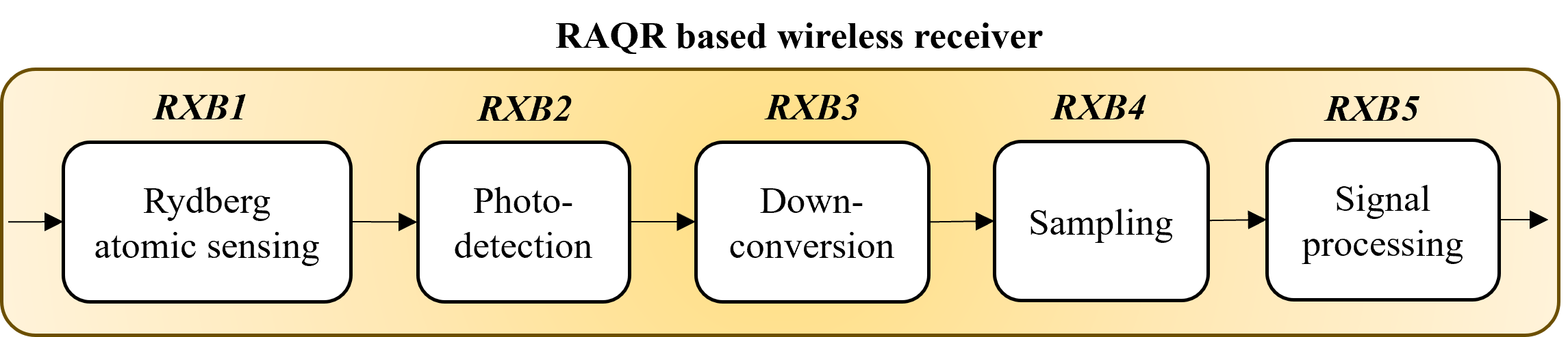
Figure 2: Illustration of the RAQR-aided wireless receiver.

We first present a detailed block diagram to illustrate the end-to-end reception process of the RAQR-aided wireless system, and then derive the corresponding end-to-end equivalent baseband signal model. The block diagram of the RAQR-aided wireless system is presented in Fig. 2.

III-B1 Rydberg Atomic Sensing

The superposition of the desired RF signal and the LO will be received by Rydberg atoms. Let us first denote the LO by $y(t)=\sqrt{2\mathcal{P}_{y}}\cos(2\pi f_{l}t+\theta_{y})=\sqrt{2}\mathscr{R}\left\{y_{b}(t)e^{\jmath 2\pi f_{l}t}\right\}$, where $\mathcal{P}_{y}$ represents the power and $y_{b}(t)=\sqrt{\mathcal{P}_{y}}e^{\jmath\theta_{y}}$ is the equivalent baseband signal. The power is given by $\mathcal{P}_{y}=\frac{1}{2}c\epsilon_{0}A_{e}\left|U_{y}\right|^{2}$, where $U_{y}$ represents the amplitude of the LO. Recall that $f_{\delta}=f_{c}-f_{l}$ and $\theta_{\delta}=\theta_{x}-\theta_{y}$ are the frequency difference and phase difference between the RF signal and the LO. Then we can formulate the incident signal superposition as follows

$$z(t)=x(t)+y(t) =\sqrt{2}\mathscr{R}\left\{\left[x_{b}(t)e^{\jmath 2\pi f_{\delta}t}+y_{b}(t)\right]e^{\jmath 2\pi f_{l}t}\right\}$$

$$\overset{(a)}{\approx}\sqrt{2\mathcal{P}_{z}}\cos(2\pi f_{l}t+\theta_{y}),$$ (15)

where $\mathcal{P}_{z}=\frac{1}{2}c\epsilon_{0}A_{e}\left|U_{z}\right|^{2}$ represents the power of $z(t)$. In the expression of $\mathcal{P}_{z}$, we have the amplitude $U_{z}$ formulated as

$$U_{z} =\sqrt{\left|U_{x}\right|^{2}+\left|U_{y}\right|^{2}+2U_{x}U_{y}\cos(2\pi f_{\delta}t+\theta_{\delta})}$$

$$\overset{(b)}{\approx}U_{y}+U_{x}\cos(2\pi f_{\delta}t+\theta_{\delta}).$$ (16)

See Appendix B for the proofs of (15) and (16). Furthermore, we obey the relationships of $\Omega_{\text{RF}}=\sqrt{A_{e}c\epsilon_{0}}U_{z}\mu_{34}/\hbar=\sqrt{2\mathcal{P}_{z}}\mu_{34}/\hbar$, $\Omega_{y}=\sqrt{A_{e}c\epsilon_{0}}U_{y}\mu_{34}/\hbar=\sqrt{2\mathcal{P}_{y}}\mu_{34}/\hbar$, and $\Omega_{x}=\sqrt{A_{e}c\epsilon_{0}}U_{x}\mu_{34}/\hbar=\sqrt{2\mathcal{P}_{x}}\mu_{34}/\hbar$, where $\mu_{34}$ represents the dipole moment corresponding to the electron transition between Rydberg states. Then the separation form of (16) facilitates the expression of the superimposed Rabi frequency $\Omega_{\text{RF}}=\Omega_{l}+\Omega_{x}\cos{(2\pi f_{\delta}t+\theta_{\delta})}$ presented in (6).

To gain deeper insights concerning the output probe beam (11), we utilize $\Omega_{l}\gg\Omega_{x}$ and perform Taylor series expansion of the equivalent baseband signal $P_{b}(\Omega_{\text{RF}},t)=\sqrt{\mathcal{P}_{1}(\Omega_{\text{RF}})}e^{\jmath\phi_{p}(\Omega_{\text{RF}})}$ in the vicinity of a given value $\Omega_{\text{RF}}=\Omega_{l}$. Ignoring the high-order terms due to the fast decay of ${\left({\Omega_{\text{RF}}-\Omega_{l}}\right)}^{n}$ and retaining the first-order term, we have the approximation $P_{b}(\Omega_{\text{RF}},t)\approx P_{b}(\Omega_{l},t)+P_{b}^{{}^{\prime}}(\Omega_{l},t)\left(\Omega_{\text{RF}}-\Omega_{l}\right)$. Consequently, the probe beam (11) is approximated by

$$P\left(\Omega_{\text{RF}},t\right) \approx\sqrt{2}\mathscr{R}\bigg{\{}\bigg{[}\sqrt{\mathcal{P}_{1}(\Omega_{l})}e^{\jmath\phi_{p}(\Omega_{l})}\bigg{]}{{e^{\jmath 2\pi{f_{p}}t}}}\bigg{\}}$$

$$-\sqrt{2}\mathscr{R}\bigg{\{}\bigg{[}\sqrt{2\mathcal{P}_{1}(\Omega_{l})\mathcal{P}_{x}}\kappa_{0}(\Omega_{l})\cos\left({2\pi f_{\delta}t+\theta_{\delta}}\right)\bigg{.}\bigg{.}$$

$$\bigg{.}\bigg{.}\;\;\times\exp\left({\jmath\phi_{p}(\Omega_{l})+\jmath\psi_{p}(\Omega_{l})}\right)\bigg{]}{{e^{\jmath 2\pi{f_{p}}t}}}\bigg{\}},$$ (17)

where we have

$$\kappa_{0}(\Omega_{l})=\frac{\pi d\mu_{34}}{\hbar\lambda_{p}}\sqrt{{{\left[{{\mathscr{I}}\{\chi^{\prime}({\Omega_{l}})\}}\right]}^{2}}+{{\left[{{\mathscr{R}}\{\chi^{\prime}({\Omega_{l}})\}}\right]}^{2}}},$$ (18)

$$\psi_{p}(\Omega_{l})=\arccos\frac{{{\mathscr{I}}\{\chi^{\prime}({\Omega_{l}})\}}}{\sqrt{{{\left[{{\mathscr{I}}\{\chi^{\prime}({\Omega_{l}})\}}\right]}^{2}}+{{\left[{{\mathscr{R}}\{\chi^{\prime}({\Omega_{l}})\}}\right]}^{2}}}},$$ (19)

$$\mathscr{R}\{\chi^{\prime}\left(\Omega_{l}\right)\}=-\frac{4N_{0}\mu_{12}^{2}}{\epsilon_{0}\hbar}{\Omega_{l}}\left[\frac{{2{A_{1}}\Omega_{l}^{2}+{A_{2}}}}{{{C_{1}}\Omega_{{l}}^{4}+{C_{2}}\Omega_{{l}}^{2}+{C_{3}}}}\right.$$

$$\left.\qquad\quad\;\;\;-\frac{\left({{A_{1}}\Omega_{{l}}^{4}+{A_{2}}\Omega_{{l}}^{2}+{A_{3}}}\right)\left({2{C_{1}}\Omega_{l}^{2}+{C_{2}}}\right)}{{{{\left({{C_{1}}\Omega_{{l}}^{4}+{C_{2}}\Omega_{{l}}^{2}+{C_{3}}}\right)}^{2}}}}\right],$$ (20)

$$\mathscr{I}\{{\chi^{\prime}}\left(\Omega_{l}\right)\}=\frac{4N_{0}\mu_{12}^{2}}{\epsilon_{0}\hbar}{\Omega_{l}}\left[\frac{{2{B_{1}}\Omega_{l}^{2}+{B_{2}}}}{{{C_{1}}\Omega_{{l}}^{4}+{C_{2}}\Omega_{{l}}^{2}+{C_{3}}}}\right.$$

$$\left.\qquad\quad\;\;\;-\frac{\left({{B_{1}}\Omega_{{l}}^{4}+{B_{2}}\Omega_{{l}}^{2}+{B_{3}}}\right)\left({2{C_{1}}\Omega_{l}^{2}+{C_{2}}}\right)}{{{{\left({{C_{1}}\Omega_{{l}}^{4}+{C_{2}}\Omega_{{l}}^{2}+{C_{3}}}\right)}^{2}}}}\right].$$ (21)

Remark 2: As seen from (17), the output probe beam contains a ‘constant’ term independent of the RF signal and a ‘varying’ term influenced by the strength, frequency, and phase of the RF signal. All the information of the desired RF signal is embedded into the amplitude of the output probe beam, which will be measured by the photodetector for recovering the full information of the desired RF signal.

III-B2 Photodetection

The probe beam will be detected by a photodetector. Next, we will study two detection schemes, namely the direct incoherent optical detection (DIOD) and the balanced coherent optical detection (BCOD) [53, Ch. 8].

DIOD: In this scheme, the output probe beam is directly received, integrated over a period, and then generates a photocurrent according to the incident beam intensity, as modelled in Fig. 3(a). We first derive the power of the equivalent baseband signal relying on (11), which is further transformed to an output photocurrent according to the relationship $I_{\text{ph}}^{\text{(D)}}(t)=\frac{\eta q}{\hbar\omega_{p}}\mathcal{P}_{b}(\Omega_{\text{RF}})$. A voltage will be produced by the photocurrent after passing through a load (assuming a unit value), which is further amplified by a low noise amplifier (LNA) (gain $G$). Consequently, the amplified voltage is expressed as

$$V^{\text{(D)}}(t) =GI_{\text{ph}}^{\text{(D)}}(t)=K\mathcal{P}_{1}(\Omega_{\rm{RF}})$$

$$\overset{(c)}{\approx}K\mathcal{P}_{1}(\Omega_{l})\Big{[}1-2\kappa_{1}(\Omega_{l})\cos{\varphi_{1}({\Omega_{l}})}\Big{.}$$

$$\Big{.}\qquad\qquad\quad\times\sqrt{2\mathcal{P}_{x}}\cos\left(2\pi f_{\delta}t+\theta_{\delta}\right)\Big{]},$$ (22)

where we have ${K\triangleq\frac{{G\eta q}}{{\hbar\omega_{p}}}}$, $\kappa_{1}(\Omega_{l})={\frac{{\pi d\mu_{34}}}{{\hbar{\lambda_{p}}}}}\left|{\mathscr{I}}\{\chi^{\prime}({\Omega_{l}})\}\right|$, and $\varphi_{1}({\Omega_{l}})=\arccos{\frac{{\mathscr{I}}\{\chi^{\prime}({\Omega_{l}})\}}{\left|{\mathscr{I}}\{\chi^{\prime}({\Omega_{l}})\}\right|}}$. The approximation in (22) is derived using Taylor series expansion in the vicinity of a given value of $\Omega_{\text{RF}}=\Omega_{l}$. Given $\Omega_{l}$, (22) is a superposition of a constant plus an RF-dependent time-varying component.

Figure 3: Illustration of two typical optical detection schemes: (a) the DIOD scheme, and (b) the BCOD scheme.

BCOD: A local optical beam exists in this scheme, as portrayed in Fig. 3(b). We assume that its carrier frequency and FWHM are identical to those of the probe beam. Then we can express the local optical beam in the form of $P_{l}(t)=\sqrt{2\mathcal{P}_{l}}\cos(2\pi f_{p}t+\phi_{l})=\sqrt{2}\mathscr{R}\left\{P_{lb}(t)e^{\jmath 2\pi f_{p}t}\right\}$, where $\mathcal{P}_{l}=\frac{\pi c\epsilon_{0}}{8\ln{2}}F_{p}^{2}\left|U_{l}\right|^{2}$ and $P_{lb}(t)=\sqrt{\mathcal{P}_{l}}e^{\jmath\phi_{l}}$. Furthermore, the probe beam and the local optical beam are combined to form two distinct optical beams, namely ${P_{1}}=\frac{1}{{\sqrt{2}}}\left[{{P_{l}}\left(t\right)-P\left({{\Omega_{{\rm{RF}}}},t}\right)}\right]$ and ${P_{2}}=\frac{1}{{\sqrt{2}}}\left[{{P_{l}}\left(t\right)+P\left({{\Omega_{{\rm{RF}}}},t}\right)}\right]$. They are detected by two photodetectors, respectively. The photocurrents generated are subtracted to obtain an output photocurrent, given by $I_{\text{ph}}^{\text{(B)}}(t)=\frac{{\eta q}}{{\hbar\omega_{p}}}\left[{{P_{lb}}\left(t\right){P_{b}^{*}}\left({{\Omega_{{\rm{RF}}}},t}\right)+P_{lb}^{*}\left(t\right)P_{b}\left({{\Omega_{{\rm{RF}}}},t}\right)}\right]$ [53]. Upon using the same resistance and LNA as in DIOD, we formulate the output voltage of the BCOD scheme as follows

$$V^{\text{(B)}}(t) =GI_{\text{ph}}^{\text{(B)}}(t)=2K\sqrt{\mathcal{P}_{l}\mathcal{P}_{1}(\Omega_{\rm{RF}})}\cos\left({\phi_{l}}-{\phi_{p}}({\Omega_{{\rm{RF}}}})\right)$$

$$\overset{(d)}{\approx}2K\sqrt{\mathcal{P}_{l}\mathcal{P}_{1}(\Omega_{l})}\Big{[}\cos\left({\phi_{l}}-{\phi_{p}}({\Omega_{l}})\right)-\kappa_{2}({\Omega_{l}})\Big{.}$$

$$\Big{.}\qquad\times\cos{\varphi_{2}({\Omega_{l}})}\sqrt{2\mathcal{P}_{x}}\cos\left({2\pi{f_{\delta}}t+{\theta_{\delta}}}\right)\Big{]},$$ (23)

where $\kappa_{2}(\Omega_{l})=\kappa_{0}(\Omega_{l})$ and ${\varphi_{2}({\Omega_{l}})}={\phi_{l}}-{\phi_{p}}({\Omega_{l}})+{\psi_{p}}({\Omega_{l}})$. See Appendix C for the proof of $(d)$. Similarly, (23) contains a constant and an RF-dependent time-varying component.

III-B3 Down-conversion

The output voltage of the photodetector is forwarded to a lock-in amplifier (LIA) to realize the down-conversion, as shown in Fig. 4. After lowpass filtering, the constant component is eliminated and the output of the LIA only includes the RF-dependent time-varying component.

Based on (22) and (23), we can extract the time-varying component of $V^{\text{(D)}}(t)$ and $V^{\text{(B)}}(t)$ in a unified form as follows

$$\tilde{V}(t) =2K\widetilde{\mathcal{P}}\kappa(\Omega_{l})\cos{\varphi({\Omega_{l}})}\sqrt{2\mathcal{P}_{x}}\cos\left({2\pi f_{\delta}t+\theta_{\delta}}\right)$$

$$=\sqrt{2}\mathscr{R}\left\{\tilde{V}_{b}(t)e^{\jmath 2\pi f_{\delta}t}\right\},$$ (24)

where we have $\widetilde{\mathcal{P}}\in\{\mathcal{P}_{1}(\Omega_{l}),\sqrt{\mathcal{P}_{l}\mathcal{P}_{1}(\Omega_{l})}\}$, $\kappa(\Omega_{l})\in\{\kappa_{1}(\Omega_{l}),\kappa_{2}(\Omega_{l})\}$, and $\varphi({\Omega_{l}})\in\{\varphi_{1}({\Omega_{l}}),\varphi_{2}({\Omega_{l}})\}$ associated with the DIOD and the BCOD, respectively. The equivalent baseband signal in (24) is formulated as

$$\tilde{V}_{b}(t) =2K\widetilde{\mathcal{P}}\kappa(\Omega_{l})\cos{\varphi({\Omega_{l}})}\sqrt{\mathcal{P}_{x}}e^{\jmath\theta_{\delta}}\triangleq\varrho\Phi x_{b}(t),$$ (25)

where $\varrho$ and $\Phi$ denote the gain and phase of RAQR, respectively, which are expressed as

$$\varrho =\begin{cases}2K\mathcal{P}_{1}(\Omega_{l})\kappa_{1}(\Omega_{l}),&\text{DIOD},\\ 2K\sqrt{\mathcal{P}_{l}\mathcal{P}_{1}(\Omega_{l})}\kappa_{2}(\Omega_{l}),&\text{BCOD},\end{cases}$$ (26)

$$\Phi =\begin{cases}\frac{e^{-\jmath\left({\theta_{y}}-\varphi_{1}({\Omega_{l}})\right)}}{2}+\frac{e^{-\jmath\left({\theta_{y}}+\varphi_{1}({\Omega_{l}})\right)}}{2},&\text{DIOD},\\ \frac{e^{-\jmath\left({\theta_{y}}-\varphi_{2}({\Omega_{l}})\right)}}{2}+\frac{e^{-\jmath\left({\theta_{y}}+\varphi_{2}({\Omega_{l}})\right)}}{2},&\text{BCOD}.\end{cases}$$ (27)

III-B4 Sampling

Sampling both sides of (25) at multiples of $1/W$ as shown in Fig. 4, we have the sampled output as

$$\tilde{V}_{b}(m) =\varrho\Phi x_{b}(m).$$ (28)

Figure 4: Illustration of the down-conversion and the sampling.

Equivalent baseband signal model for communications: Upon replacing $x_{b}(m)$ by $s_{b}$ based on (13), we arrive at the equivalent baseband signal model of wireless communications in the form of

$$\tilde{V}_{b}(m) =\sqrt{A_{e}}\varrho\Phi\sum_{\ell}h_{\ell}(m)s_{b}(m-\ell),$$ (29)

where $h_{\ell}(m)$ is shown as a complex Gaussian random variable exhibiting the circular symmetry property, namely, $h_{\ell}(m)\sim\mathcal{CN}(0,\sigma_{\ell}^{2})$ [51, Ch. 2]. Furthermore, upon adding the additive noise (denoted by $w(m)$) to (29), we formulate the noisy discrete-time baseband signal model as follows

$$\tilde{V}_{b}(m)=\sqrt{A_{e}}\varrho\Phi\sum_{\ell}h_{\ell}(m)s_{b}(m-\ell)+w(m).$$ (30)

Even if (30) is capable of depicting the wideband systems, we emphasize that RAQRs have a narrow instantaneous bandwidth of $\leq 10$ MHz [31], where only a small frequency range around the resonant frequency can be closely coupled. Based on this situation, we provide the following equivalent baseband signal model for narrowband systems

$$\tilde{V}_{b}(m)=\sqrt{A_{e}}\varrho\Phi h_{\text{com}}(m)s_{b}(m)+w(m),$$ (31)

where $h_{\text{com}}(m)=h_{\ell=0}(m)\sim\mathcal{CN}(0,\sigma_{\ell=0}^{2})$.

Equivalent baseband signal model for sensing: Upon replacing $x_{b}(m)$ by $s_{b}$ based on (14), we have the equivalent baseband signal model in the form of

$$\tilde{V}_{b}(m) =\sqrt{A_{e}}\varrho\Phi h_{\text{sen}}(m)s_{b}\left(m-\frac{2\left(R_{0}-vpT\right)}{c}\right),$$ (32)

where $h_{\text{sen}}(m)=a(m)$. We assume $U_{s}\left(t-pT-t_{d}\right)\approx U_{s}(t-pT)$, implying that the amplitude of $s_{b}$ is constant over the round-trip period of $t_{d}=\frac{2(R_{0}-vpT)}{c}$. Then we have $s_{b}\left(m-\frac{2(R_{0}-vpT)}{c}\right)\approx e^{-\jmath\frac{4\pi f_{c}}{c}(R_{0}-vpT)}s_{b}(m)$, where the phase shift $e^{-\jmath\frac{4\pi f_{c}}{c}(R_{0}-vpT)}$ can be integrated into $h_{\text{sen}}(m)$. Therefore, we have the noisy form of (32) as follows

$$\tilde{V}_{b}(m) =\sqrt{A_{e}}\varrho\Phi\bar{h}_{\text{sen}}(m)s_{b}\left(m\right)+w(m),$$ (33)

where $\bar{h}_{\text{sen}}(m)=a(m)e^{-\jmath\frac{4\pi f_{c}}{c}(R_{0}-vpT)}$.

Remark 3: It is seen from both models for communications and sensing that the RAQR imposes a gain $\varrho$ and a phase shift $\Phi$ to the RF signal. These parameters are determined by both the atomic response and the photodetection scheme selected. Particularly, the phase shift may be integrated into $h(m)\in\{h_{\text{com}}(m),h_{\text{sen}}(m),\bar{h}_{\text{sen}}(m)\}$ to form an equivalent wireless channel $\Phi h(m)$. For communication purposes, upon exploiting the circular symmetry property, we have $\Phi h(m)\sim\mathcal{CN}(0,\sigma_{\ell}^{2})$ for any given $\Phi\in\{\Phi_{1},\Phi_{2}\}$.

III-C Noise Sources in RAQR-Aided Wireless Systems

In this part, we focus our attention on the noise sources that affect the RAQR both extrinsically and intrinsically.

III-C1 Extrinsic Noise Source

The black-body radiation induced extrinsic thermal noise (ETN) is included in this category. Upon assuming an electrically large enclosure of the volume formed by media at temperature $T$ that surround the receiver, we formulate the intensity of the ETN as $\mathcal{P}_{\text{EN}}=\frac{1}{2}c\rho_{v}n(\omega_{x},T)\hbar\omega_{x}$ [41], where $\rho_{v}=8\pi f_{c}^{2}/c^{3}$ represents the volumetric and spectral density of modes and $\omega_{x}=2\pi f_{c}$ is the angular frequency. Specifically, $n(\omega_{x},T)$ obeys the boson Bose-Einstein distribution $n(\omega_{x},T)=$ ${1\mathord{\left/{\vphantom{1{\left({\exp\left({\frac{{\hbar{\omega_{x}}}}{{{k_{B}}T}}}\right)-1}\right)}}}\right.\kern-1.2pt}{\left({\exp\left({\frac{{\hbar{\omega_{x}}}}{{{k_{B}}T}}}\right)-1}\right)}}$ [41], where $k_{B}$ is the Boltzmann constant.

It is worth noting that $\mathcal{P}_{\text{EN}}$ represents the total intensity of both the electric and magnetic fields, and it is for triple-polarization. In our system, we assume that the RAQR only receives the electric field in single polarization. Therefore, the intensity of the ETN becomes $\mathcal{P}_{\text{en}}=\frac{1}{6}\mathcal{P}_{\text{EN}}$. Note that the ETN will be amplified by the LNA of the photodetector. Given the effective receiver aperture $A_{e}$ and the LNA gain $G$, the power of the extrinsic noise imposed on the baseband signal $\tilde{V}_{b}(m)$ across bandwidth $B\ll f_{c}$ is derived as

$$N_{\text{extrinsic}}=G^{2}A_{e}\mathcal{P}_{\text{en}}B=G^{2}\frac{c\hbar\omega_{x}\rho_{v}}{12}n(\omega_{x},T)A_{e}B.$$ (34)

III-C2 Intrinsic Noise Sources

Several different intrinsic noise sources are considered as follows.

Photodetector’s shot noises (PSNs): Consider a PIN photodiode, then two shot noise sources arise in the photodetector, namely, the photon shot noise and the dark-current shot noise. For the DIOD scheme, upon denoting the average photocurrent and the average dark-current by $\bar{I}_{\text{ph}}$ and $\bar{I}_{\text{d}}$, respectively, where $\bar{I}_{\text{ph}}=\frac{{\eta q}}{{\hbar\omega_{p}}}\mathcal{P}_{1}(\Omega_{l})$, we formulate the noise power of the PSNs (after LNA) across bandwidth $B$ as follows [42, Ch. 5]

$$N_{\text{shot}}^{\text{(D)}}=2qB\left(\bar{I}_{\text{ph}}+\bar{I}_{\text{d}}\right)G^{2}.$$ (35)

For the BCOD scheme, let us denote the average photocurrents generated by the two photodetectors by $\bar{I}_{\text{ph}}^{\text{(1)}}$ and $\bar{I}_{\text{ph}}^{\text{(2)}}$, respectively. They correspond to $P_{1}$ and $P_{2}$, respectively, and are formulated as $\bar{I}_{\text{ph}}^{\text{(1)}}=\bar{I}_{\text{ph}}^{\text{(2)}}=\frac{{\eta q}}{{2\hbar\omega_{p}}}\mathcal{P}_{l}$. Upon assuming that the dark-currents generated in the two photodetectors are at the same power level, we formulate the noise power of the PSNs (after LNA) across bandwidth $B$ as follows [53, Ch. 8], [42, Ch. 5]

$$N_{\text{shot}}^{\text{(B)}}=2qB\left(\bar{I}_{\text{ph}}^{\text{(1)}}+\bar{I}_{\text{ph}}^{\text{(2)}}+2\bar{I}_{\text{d}}\right)G^{2}.$$ (36)

Intrinsic thermal noise (ITN): It is also known as the Johnson noise and it is induced by the random motions of conduction electrons. The ITN power across bandwidth $B$ is given by

$$N_{\text{thermal}}=4k_{\text{B}}TB.$$ (37)

Note that the ITN produced in the system comes from the LNA, LIA, and the remaining electronic components, e.g., ADCs. Therefore, $T$ becomes an equivalent noise temperature characterizing the combined effect of all these components. Based on [43, Ch. 16], the noise temperature of the LNA dominates, namely, we have $T\approx T_{\text{LNA}}$.

Quantum projection noise (QPN): QPN is also known as the atomic shot noise, which is inevitably produced due to the probabilistic collapse of the wavefunction during its measurements. It is governed by the SQL, which reveals that, when measuring with $N$ quantum-mechanically uncorrelated atoms, the probabilistic collapse from a superposition state to either eigenstate of each atom wavefunction results in the limit of phase measurement, given by $\varphi=\varphi_{\text{SQL}}=\frac{1}{\sqrt{N}}$ [44, 16, 45]. One may employ an extremely large number of Rydberg atoms to reduce this noise so that it can be reasonably neglected.

III-C3 Total Noise Power

Based on the above discussions, we model $w(m)$ in (30), (31) and (33) as a complex additive white Gaussian noise process obeying $w(m)\sim\mathcal{CN}(0,\sigma_{w}^{2})$, where

$$\sigma_{w}^{2}=N_{\text{extrinsic}}+N_{\text{shot}}+N_{\text{thermal}}.$$ (38)

IV Performance Analysis and Comparison

In this section, we study the receive SNR of a narrowband RAQR-aided wireless system. One can further derive the capacity (spectral efficiency) and/or study the bit-error-rate of an RAQR-aided communication system based on the receive SNR. Relying on (31), (33), and (38), we formulate the SNR of the receive signal in (39) at the top of next page, where $h(m)\in\{h_{\text{com}}(m),h_{\text{sen}}(m)\}$.

$$\mathsf{SNR} =\frac{|\sqrt{A_{e}}\varrho\Phi h(m)|^{2}}{\sigma_{w}^{2}}\mathcal{P}_{s}=\left\{\begin{aligned} &{\frac{{A_{e}\varrho_{1}^{2}\cos^{2}{\varphi_{1}({\Omega_{l}})}|{h}(m){|^{2}}{{\cal P}_{{s}}}}}{G^{2}A_{e}{{\cal P}_{{\rm{en}}}}B+qBG\left({2K{{\cal P}_{1}}({\Omega_{l}})}+2{{\bar{I}}_{\rm{d}}}RG\right)+4{k_{\rm{B}}}TB}},&&{{\rm{DIOD}}}.\\ &{\frac{{A_{e}\varrho_{2}^{2}\cos^{2}{\varphi_{2}({\Omega_{l}})}|{h}(m){|^{2}}{{\cal P}_{{s}}}}}{G^{2}A_{e}{{\cal P}_{{\rm{en}}}}B+qBG\left({2K{{\cal P}_{l}}}+4{{\bar{I}}_{\rm{d}}}RG\right)+4{k_{\rm{B}}}TB}},&&{{\rm{BCOD}}}.\\ \end{aligned}\right.$$ (39)

To simplify the SNR expression, the dark-current term can be reasonably neglected because it is relatively small compared to its photocurrent counterpart. Additionally, $\cos^{2}{\varphi_{1}({\Omega_{l}})}=1$ always holds and one may configure the phase of the local optical beam $\phi_{l}$ to retain $\varphi_{2}(\Omega_{l})=0$, so that $\cos^{2}{\varphi_{2}({\Omega_{l}})}=1$. Based on these discussions, we approximate (39) to

$$\overline{\mathsf{SNR}} \approx\frac{{{A_{e}}{\varrho^{2}}|{h}(m){|^{2}}{{\cal P}_{{s}}}}}{{G^{2}{A_{e}}{{\cal P}_{{\rm{en}}}}B+2qBGK{\cal P}+4{k_{\rm{B}}}TB}},$$ (40)

where $\mathcal{P}\in\{\mathcal{P}_{1}(\Omega_{l}),\mathcal{P}_{l}\}$ corresponds to the DIOD and the BCOD, respectively. In the RAQR paradigm, PSN may become the dominant noise (one can verify this via simple numerical comparison between PSN and other noise sources). Therefore, the SNR can be further simplified to

$$\overline{\mathsf{SNR}}_{1} \approx\frac{{{A_{e}}{\varrho^{2}}|{h}(m){|^{2}}{{\cal P}_{{s}}}}}{2qBGK{\cal P}}$$

$$=\begin{cases}\frac{{2\eta}}{{\hbar\omega_{p}}}\frac{A_{e}}{B}{\mathcal{P}_{1}(\Omega_{l})\kappa_{1}^{2}(\Omega_{l})}|{h}(m){|^{2}}{{\cal P}_{s}}&\text{DIOD},\\ \frac{{2\eta}}{{\hbar\omega_{p}}}\frac{A_{e}}{B}{\mathcal{P}_{1}(\Omega_{l}){\kappa_{2}^{2}}({\Omega_{l}})}|{h}(m){|^{2}}{{\cal P}_{s}}&\text{BCOD}.\end{cases}$$ (41)

Remark 4: It is seen from (41) that $\overline{\mathsf{SNR}}_{1}$ is independent of ${\cal P}_{l}$ for the BCOD scheme and it is also independent of the LNA gain $G$ of both schemes. It is determined by the product of $\mathcal{P}_{1}(\Omega_{l})$ and $\kappa^{2}(\Omega_{l})$, $\kappa(\Omega_{l})\in\{\kappa_{1}(\Omega_{l}),\kappa_{2}(\Omega_{l})\}$ for a given $A_{e}$, $B$, and the channel ${h}(m)$. To achieve higher receive SNR, one may (jointly) optimize the frequency detuning and power of the probe, coupling, and LO signals to obtain an optimal product of $\mathcal{P}_{1}(\Omega_{l})$ and $\kappa^{2}(\Omega_{l})$, which will be our future work.

We then compare DIOD and BCOD based on the SNR ratio $\overline{\mathsf{Ratio}}=\overline{\mathsf{SNR}}_{\rm{(BCOD)}}/\overline{\mathsf{SNR}}_{\rm{(DIOD)}}$. Based on (40), we obtain

$$\overline{\mathsf{Ratio}} ={\left({\frac{{{\varrho_{2}}}}{{{\varrho_{1}}}}}\right)^{2}}\frac{{{G^{2}{\cal P}_{{\rm{en}}}}+\frac{{2qGK{{\cal P}_{1}}({\Omega_{l}})+4{k_{\rm{B}}}T}}{{{A_{e}}}}}}{{{G^{2}{\cal P}_{{\rm{en}}}}+\frac{{2qGK{{\cal P}_{l}}+4{k_{\rm{B}}}T}}{{{A_{e}}}}}}$$

$$={\left({\frac{{{\kappa_{2}}({\Omega_{l}})}}{{{\kappa_{1}}({\Omega_{l}})}}}\right)^{2}}\frac{{\frac{{{G^{2}{\cal P}_{{\rm{en}}}}}}{{{{\cal P}_{1}}({\Omega_{l}})}}+\frac{{2qGK}}{{{A_{e}}}}+\frac{{4{k_{\rm{B}}}T}}{{{{\cal P}_{1}}({\Omega_{l}}){A_{e}}}}}}{{\frac{{{G^{2}{\cal P}_{{\rm{en}}}}}}{{{{\cal P}_{l}}}}+\frac{{2qGK}}{{{A_{e}}}}+\frac{{4{k_{\rm{B}}}T}}{{{{\cal P}_{l}}{A_{e}}}}}}\geq 1,$$ (42)

where $\overline{\mathsf{Ratio}}\geq 1$ is due to ${\kappa_{1}}({\Omega_{l}})\leq{\kappa_{2}}({\Omega_{l}})$ and $\mathcal{P}_{l}\geq\mathcal{P}_{1}({\Omega_{l}})$, suggesting that the BCOD scheme always outperforms the DIOD scheme in terms of the receive SNR. To gain deeper insights, we consider the PSN dominant case, namely $2qBGK{\cal P}\gg\max\{G^{2}{A_{e}}{{\cal P}_{{\rm{en}}}}B,4{k_{\rm{B}}}TB\}$, then the SNR ratio can be further simplified to

$$\overline{\mathsf{Ratio}}_{1} ={\left({\frac{{{\kappa_{2}}({\Omega_{l}})}}{{{\kappa_{1}}({\Omega_{l}})}}}\right)^{2}}=1+{{\left(\frac{{{\mathscr{R}}\{\chi^{\prime}({\Omega_{l}})\}}}{{{\mathscr{I}}\{\chi^{\prime}({\Omega_{l}})\}}}\right)}^{2}}\geq 1.$$ (43)

Remark 5: When considering the ‘no detuning’ case of the laser beams and the LO, namely $\Delta_{p}=\Delta_{c}=\Delta_{l}=0$, we obtain ${\mathscr{R}}\{\chi^{\prime}({\Omega_{l}})\}=0$, so that $\overline{\mathsf{Ratio}}_{1}=1$ always holds. This reveals that the receive SNR of the DIOD scheme is exactly the same as that of the BCOD scheme, as it will be observed in our simulation results, where the curve of BCOD coincides with that of the DIOD. It is emphasized that ${\mathscr{R}}\{\chi^{\prime}({\Omega_{l}})\}\neq 0$ and the BCOD scheme always achieves a higher receive SNR than that of the DIOD scheme, when the frequency detuning parameters are optimized instead of being fixed to zero.

IV-A Comparisons to Conventional RF Receivers

IV-A1 Signal Model of Conventional RF Receivers

Before comparing the RAQRs to the conventional RF receivers, we follow [43, Ch. 16] and present a typical single-antenna reception structure for the conventional RF receivers in Fig. 5. The system consists of an antenna (gain $G_{\text{Ant}}$ and noise temperature $T_{\text{Ant}}$), an LNA (gain $G_{\text{LNA}}$ and noise temperature $T_{\text{LNA}}$), and the remaining components (equivalent gain $G_{\text{REC}}$ and equivalent noise temperature $T_{\text{REC}}$), such as transmission lines, mixers, lowpass filters and ADCs. Upon considering the narrowband systems, we derive the input-output equivalent baseband signal model as follows

$$\tilde{V}_{0}(m)=\sqrt{A_{\text{ant}}}\varrho_{0}h(m)s_{b}(m)+w_{0}(m),$$ (44)

where $\varrho_{0}=G_{\text{Ant}}G_{\text{LNA}}G_{\text{REC}}$ represents the gain of the conventional RF receivers, $A_{\text{ant}}$ is the effective receiver aperture of the antenna, and $w_{0}$ is the AWGN of the RF receiver. Specifically, the noise includes the ETN and the ITN, where the ETN will be amplified by the LNA of the system. Then, we have $w(m)\sim\mathcal{CN}(0,N_{\text{RF}})$ with $N_{\text{RF}}=G_{\text{LNA}}^{2}A_{\text{ant}}\mathcal{P}_{\text{en}}B+4k_{\text{B}}T_{\text{E}}B$, where $T_{\text{E}}$ is the equivalent noise temperature of the whole system excluding the antenna, given by $T_{\text{E}}=T_{\text{LNA}}+\frac{1}{G_{\text{LNA}}}T_{\text{REC}}$ [43, Ch. 16]. When employing high-gain LNAs, one can neglect the second term of $T_{\text{E}}$ because it is comparably small. Based on these discussions, we formulate the receive SNR as

$$\mathsf{SNR}_{0} \approx\frac{{{A_{{\rm{ant}}}}\varrho_{0}^{2}|{h}(m){|^{2}}{{\cal P}_{{s}}}}}{G_{\text{LNA}}^{2}{A_{{\rm{ant}}}}{{\cal P}_{{\rm{en}}}}B+4{k_{\rm{B}}}{T_{{\rm{LNA}}}}B}.$$ (45)

Figure 5: Illustration of the conventional RF receiver.

IV-A2 Comparison Between RAQRs and Conventional RF Receivers

We compare them in terms of the SNR ratio. Based on (40) and (45), we formulate the SNR ratio as

$$\mathsf{Ratio}_{0}=\frac{\overline{\mathsf{SNR}}}{\mathsf{SNR}_{0}}={\left({\frac{\varrho}{{{\varrho_{0}}}}}\right)^{2}}\frac{{{{{G_{{\rm{LNA}}}^{2}}}{\cal P}_{{\rm{en}}}}+\frac{{4{k_{\rm{B}}}{T_{{\rm{LNA}}}}}}{{{A_{{\rm{ant}}}}}}}}{{{G^{2}{\cal P}_{{\rm{en}}}}+\frac{{2qGK{\cal P}+4{k_{\rm{B}}}T}}{{{A_{e}}}}}}.$$ (46)

$\mathsf{Ratio}_{0}\geq 1$ implies that the SNR achieved by the RAQRs is greater than that achieved by the conventional RF receivers. To obtain this SNR gain, we formulate the following lower bound condition (LBC)

$$\varrho \geq{\varrho_{0}}\sqrt{\frac{{{A_{{\rm{ant}}}}}}{{{A_{e}}}}}\sqrt{\frac{{G^{2}{A_{e}}{{\cal P}_{{\rm{en}}}}+2qGK{\cal P}+4{k_{\rm{B}}}T}}{{{G_{{\rm{LNA}}}^{2}}{A_{{\rm{ant}}}}{{\cal P}_{{\rm{en}}}}+4{k_{\rm{B}}}{T_{{\rm{LNA}}}}}}}.$$ (47)

The interpretation of the LBC is that the RAQR gain should be greater than the right side of the inequality to show their superiority over the conventional RF receivers. Furthermore, (47) also serves as a criterion for the assessment of diverse parameters, such as the LNA gain, the noise temperature, and the receiver aperture. When considering the special case, where $A_{e}=A_{\text{ant}}$, $G=G_{\rm{LNA}}$, and $T=T_{\rm{LNA}}$, we further reformulate (47) to

$$\varrho \geq{\varrho_{0}}\sqrt{1+\frac{{2q{G_{{\rm{LNA}}}}K{\cal P}}}{{{G_{{\rm{LNA}}}^{2}}{A_{{\rm{ant}}}}{{\cal P}_{{\rm{en}}}}+4{k_{\rm{B}}}{T_{{\rm{LNA}}}}}}}.$$ (48)

The LBC in (48) can be a metric for comparing the RAQRs to the conventional RF receivers in terms of the identical receiver aperture and the identical LNA gain and noise temperature.

IV-A3 Effective Receiver Aperture

Assuming that the laser beams are Gaussian beams, we approximate the receiver aperture, where the probe/coupling beams are spatially-overlapped in the vapor cell, as a cylinder. The effective receiver aperture of RAQRs $A_{e}$ is the surface area of the cylinder. Upon assuming that the FWHMs of the probe and coupling beams are identical, and the radius of the cylinder is given by $r_{0}=F_{p}/\sqrt{2\ln{2}}$, we obtain RAQR’s effective receiver aperture as $A_{e}=\frac{\pi F_{p}^{2}}{\ln{2}}+\sqrt{\frac{2}{\ln{2}}}\pi dF_{p}$. We employ a $\lambda/2$-spaced dipole antenna in the conventional RF benchmark receivers. The maximum effective receiver aperture of such a dipole antenna is provided by its physical area, i.e., $A_{\text{ant}}=\lambda^{2}/(4\pi)$. Upon comparing the RAQRs and the half-wavelength dipole antenna, we observe that the former’s effective receiver aperture is determined by both the laser’s radius and the vapor cell’s length, while the latter’s is only related to the wavelength of the RF receive signal.

V Simulation Results

V-A Simulation Configurations

Upon following the configurations in [18], we consider a vapor cell (length $d=2$ cm) filled up with Cs atoms that has an atomic density of $N_{0}=4.89\times 10^{10}\text{cm}^{-3}$. To build a four-level scheme, the probe beam having a wavelength of $852$ nm and a beam diameter of $1.7$ mm excites the atoms from the ground state 6S _1/2 to the excited state 6P _3/2 . The power of the probe beam at the access point of the atoms is $29.8$ µW, which corresponds to a Rabi frequency of $2\pi\times 5.7$ MHz. The coupling beam excites the atoms from 6P _3/2 to the Rydberg state 47D _5/2 , where the wavelength and beam diameter are $510$ nm and $1.7$ mm, respectively. The power of the coupling beam at the access point of the atoms is $17$ mW, corresponding to a Rabi frequency of $2\pi\times 0.97$ MHz. The LO signal is configured with a carrier frequency of $6.9458$ GHz to couple the Rydberg states 47D _5/2 and 48P _3/2 . The desired RF signal to be received is near this transition frequency, with a small frequency offset of $150$ kHz. The powers of the LO and the desired RF signal are $10$ dBm and $-150$ dBm, respectively. In this article, we consider a bandwidth of $1$ MHz, which is within the typical value of atomic responses $<10$ MHz [31]. The decay rates of the four energy levels are $\gamma=0$, $\gamma_{2}=2\pi\times 5.2$ MHz, $\gamma_{3}=2\pi\times 3.9$ kHz, and $\gamma_{4}=2\pi\times 1.7$ kHz, respectively. The decay rates related to the collisions are ignored, yielding $\gamma_{c}=0$.

For fair comparison, a single half-wavelength dipole antenna is employed for the conventional RF receivers, which is widely used and generally serves as the gain standard. It is isotropic and has a gain around $G_{\text{Ant}}=2.1$ dB [54, Ch. 17]. Recall from [55] that the LNA gains at various frequencies obey $\leq 30$ dB. We thus set $G_{\text{LNA}}=30$ dB as the benchmark. For the conventional RF receivers, we assume $G_{\text{REC}}=0$ dB. We select a typical LNA noise temperature of $T_{\text{LNA}}=100$ Kelvin [41]. In the photodetection stage of the RAQRs, the quantum efficiency is configured as $\eta=0.8$. The LNA used in the photodetector has a gain of $G=30$ dB and a noise temperature of $T=100$ Kelvin.

Unless otherwise stated, our simulations will follow the above configurations. We will first validate the correctness of our model, and then simulate the effects of several critical parameters on the receive SNR (40), the gain (26) of RAQR-DIOD and RAQR-BCOD, respectively, and the gain of LBC (47). In all simulations, we present:

1. The effective receiver aperture of the RAQRs obeying the above configuration, which is different from that of the dipole antenna, namely $A_{e}\neq A_{\text{ant}}$.

2. The effective receiver aperture of the RAQRs is configured the same as that of the dipole antenna, namely $A_{e}=A_{\text{ant}}$.

Additionally, in the receive SNR simulations, we present:

1. The standard (unoptimized) case, where the detunings are $\Delta_{p/c/l}=0$ and the probe beam power is $29.8$ µW.

2. The optimized case, where the detunings and probe beam power are numerically optimized. The detunings are obtained as $\Delta_{p}=2\pi\times(-3.7)$ MHz, $\Delta_{l}=2\pi\times 0.02$ MHz, and $\Delta_{c}=2\pi\times$($1.92$, $2.04$, $2.16$, $2.3$, $1.36$, $1.54$) MHz for the carrier frequencies of $6.9458$, $7.9752$, $9.2186$, $11.6187$, $13.4078$, $15.5513$ GHz. The probe beam power is $9.4$ µW.

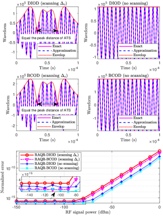
Figure 6: The waveforms and the normalized approximation error of the proposed signal model.

V-B Validation of the Proposed Signal Model

We validate our signal model by showing the coincidence of waveforms between the time-varying component (24) constructed by our model and the exact one obtained by removing the constant component of (11). We then quantify the normalized approximation error between the approximate probe beam (17) and the exact probe beam (11). We select an observation window of $0.1$ ms to capture the waveforms, during which we keep the amplitude of the RF signal constant. We also consider two cases: ① Scan $\Delta_{c}$ from $2\pi\times(-4)$ MHz to $2\pi\times 4$ MHz during the observation window, while keeping $\Delta_{p}=\Delta_{l}=0$; ② Fix $\Delta_{p}=\Delta_{c}=\Delta_{l}=0$ without any scanning. The results obtained are shown in Fig. 6.

It is observed from Fig. 6 that the approximate and exact waveforms coincide for both the scanning and no-scanning cases. The envelopes of the exact waveforms can be accurately captured in both cases. Note that the waveforms of the scanning-based scenario exhibit a time-varying envelop related to the Autler–Townes splitting [9, 10, 11, 12] of the probe beam, as indicated in the scanning-based sub-figures. This is because the envelope of the DIOD scheme is changed by $\kappa_{1}({\Omega_{l}})$ when scanning $\Delta_{c}$. By contrast, the waveforms of the no-scanning case have a constant envelope. We then observe from Fig. 6 that the normalized approximation errors related to the two cases appear to be flat below a critical point (around $-80$ dBm) of the RF signal’s power, and gradually increase after the critical point. This is because the approximation error of $U_{z}\approx U_{y}+U_{x}\cos(2\pi f_{\delta}t+\theta_{\delta})$ gradually increases as the RF signal’s power increases compared to a fixed-power LO ($10$ dBm), which causes an increased error for the approximate probe beam. Overall, the errors are small enough and can be controlled, while satisfying the condition of $\mathcal{P}_{y}\gg\mathcal{P}_{x}$.

V-C Performance of the RAQR-Aided Wireless Systems

Performance Versus (vs.) Atomic Density: Upon fixing all other parameters and varying the atomic density with $N_{0}=(1\sim 9)\times 10^{10}$ $\text{cm}^{-3}$, we plot the curves in Fig. 9.

It is observed that the receive SNR of RAQR logarithmically increases in dB vs. the atomic density. Both the S1 and S2 cases of RAQR under the unoptimized state (S3) outperform the half-wavelength dipole antenna based conventional RF receiver across the entire atomic density range, as observed from Fig. 9(a). More particularly, when the atomic density is $5\times 10^{10}$ $\text{cm}^{-3}$ (near the configuration of $N_{0}=4.89\times 10^{10}\text{cm}^{-3}$ in [18]), the S1 and S2 cases under the S3 configuration exhibit $\sim 22.6$ dB and $\sim 29$ dB gain over the conventional RF receiver, respectively, as portrayed in Fig. 9(a).

Another observation of the S1 and S2 cases under S3 is that the gain of the BCOD is higher than that of the DIOD, as seen in Fig. 9(b). However, the receive SNR of the BCOD is similar to that of the DIOD in Fig. 9(a). The extra gain of the BCOD does not result in the increase of the receive SNR. This is explained in the Remark 5 of Section IV, where the PSN dominates among all noise sources and the S3 is associated with $\Delta_{p}=\Delta_{c}=\Delta_{l}=0$.

The extra receive SNR gain of the RAQR can be further improved for the S1 and S2 cases under the optimized state S4. As depicted in Fig. 9(a), the extra receive SNR gains of the S1 case under S4 become $\sim 29$ dB and $\sim 33.5$ dB for the DIOD and the BCOD, respectively, exhibiting an increment of $\sim 6.4$ dB and $\sim 10.9$ dB over the $\sim 22.6$ dB of the unoptimized case, respectively. Note that the BCOD always outperforms the DIOD under the S4 configuration. We emphasize that our results are consistent with that in [21], which shows that RAQRs exhibit $100$ to $10000$ times ($40$ dB to $80$ dB) higher sensitivity than dipole antennas in detecting electric fields.

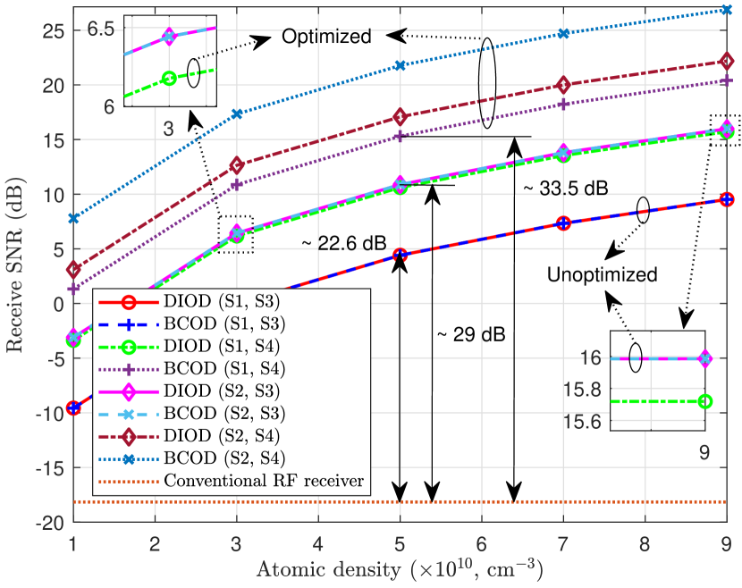
(a)

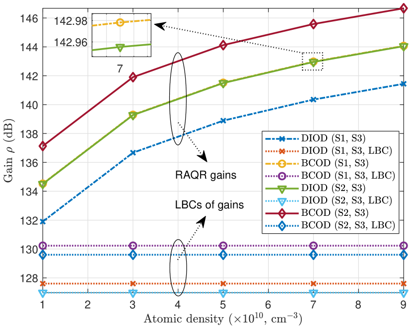
(b)

Figure 7: The receive SNR and RAQR gain vs. the atomic density.

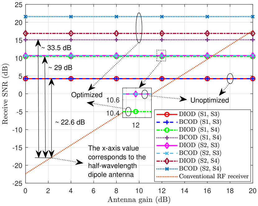
(c)

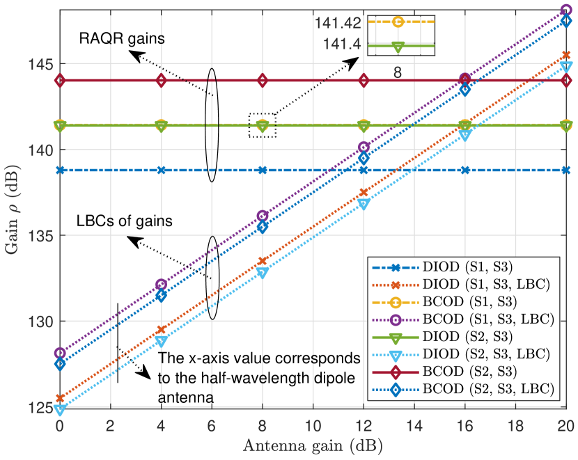
(d)

Figure 8: The receive SNR and RAQR gain vs. the antenna gain.

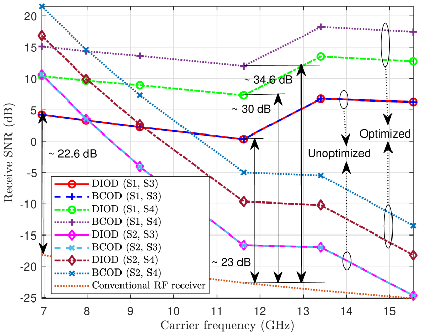
(a)

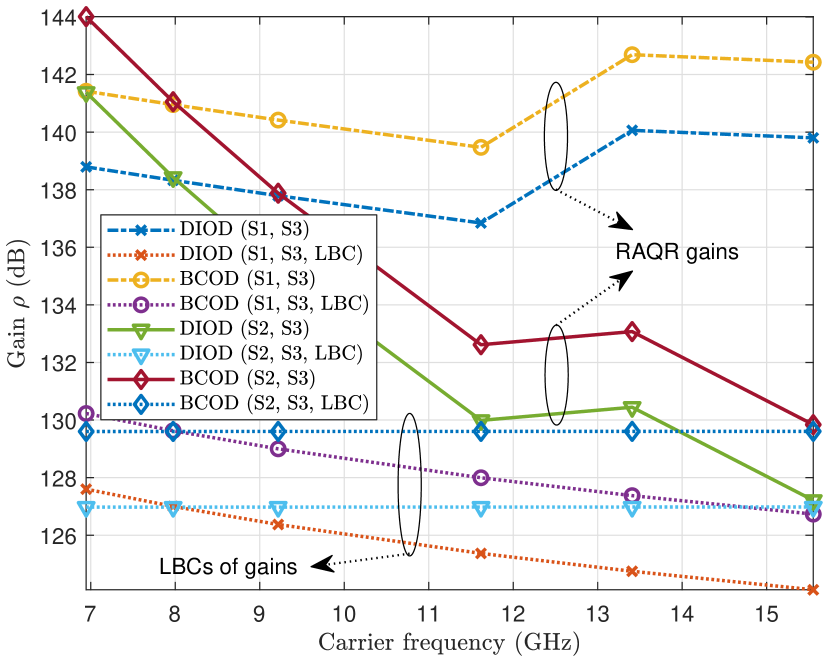
(b)

Figure 9: The receive SNR and RAQR gain vs. the carrier frequency.

Performance vs. Antenna Gain: We fix all other parameters and vary the antenna gain from $0$ dB to $20$ dB. This influences the receive SNR of the conventional RF receiver, as shown in Fig. 9(a), and affects the LBC of the RAQR gain, as depicted in Fig. 9(b). From both sub-figures that the receive SNRs and the RAQR gains remain constant across the entire range of the antenna gain, once the other parameters are given. It is observed that the DIOD and BCOD in both the S1 and S2 cases under the S3 and S4 configurations outperform the conventional RF receivers in terms of the receive SNR across a large range studied, as seen in Fig. 9(a). The RAQR gains satisfy their corresponding LBCs across this range to guarantee the superiority of RAQRs, as seen in Fig. 9(b). Notably, the half-wavelength dipole antenna has been marked in both sub-figures, where its receive SNR is significantly lower than that of the RAQR, exhibiting a gap of $\sim 22.6$ dB and $\sim 29$ dB to the S1 and S2 cases under the S3 configuration, respectively. The gaps are further enlarged under the optimized configuration S4. As marked in Fig. 9(a), these gaps become $\sim 29$ dB and $\sim 33.5$ dB in the S1 case under the S4 configuration for the DIOD and the BCOD, respectively.

Performance vs. Carrier Frequency: It is worth noting that the RAQRs are limited to receiving RF signals at specific discrete frequencies that are coupled to different but specific transitions between two Rydberg states. We follow the configurations of Cs atoms in [56, TABLE I] for receiving different carrier frequencies, namely $6.9458$, $7.9752$, $9.2186$, $11.6187$, $13.4078$, $15.5513$ GHz. The transition from the ground state to the excited state is 6S _1/2 →6P _3/2 , which is realized obeying the same configurations of the laser beams as stated above. The simulation results are presented in Fig. 9.

Let us observe the RAQR of the S1 case under the S3 and S4 configurations in Fig. 9(a), the curves slightly decrease from $6.9458$ GHz to $11.6187$ GHz, then suddenly increase from $11.6187$ GHz to $13.4078$ GHz, and become flat at the rest of the frequency range. The trend is mainly determined by the dipole moment, but is less related to the carrier frequency. The higher the dipole moment, the higher the receive SNR. By contrast, the receive SNR of the conventional RF receiver gradually drops vs. the carrier frequency. This trend is essentially due to the reduction of its effective receiver aperture. The SNR difference between the DIOD (BCOD) of the (S1, S3) case and the conventional RF receiver exceeds $\sim 22.6$ dB and becomes larger with the increase of the carrier frequency, as seen in Fig. 9(a). This trend holds for the DIOD and the BCOD of the (S1, S4) case, but the SNR differences are further augmented to $\sim 30$ dB for the DIOD and $\sim 34.6$ dB for the BCOD at the $11.6187$ GHz.

For the S2 case under the S3 and S4 configurations, we observe that the receive SNRs of the DIOD and BCOD drop substantially vs. the increase of the carrier frequencies. Our explanation is that higher carrier frequencies correspond to the reduced effective receiver apertures of RAQRs (holding $A_{e}=A_{\text{ant}}$) that further reduce the number of participating Rydberg atoms (note that the atomic density keeps constant). This is why these curves drop dramatically. Even if the attenuation is significant in this case, it still remarkably outperforms the conventional RF receivers across the frequency range studied. We emphasize that the effective receiver aperture of RAQRs is preferably fixed in practical applications. Similar trends can be observed from Fig. 9(b) for the RAQR gain. More particularly, the S1 and S2 cases of both the DIOD and BCOD schemes always have higher gains than their corresponding LBCs, respectively. This guarantees the superiority of RAQRs over the conventional RF receivers across the frequencies studied.

VI Conclusions

In this article, we have proposed an end-to-end RAQR-aided wireless receiver scheme by presenting its functional blocks and constructed a corresponding equivalent baseband signal model. Our model follows a realistic signal reception flow and takes into consideration the actual implementation of the RAQRs, which makes our model practical. The proposed scheme and model may be readily harnessed for system design and signal processing for future RAQR-aided wireless communications and sensing. We have further studied the DIOD and BCOD photodetection schemes, and have theoretically demonstrated that the BCOD scheme always outperforms the DIOD scheme. We have also compared the RAQRs to the conventional RF receivers and shown the superiority of RAQRs in achieving a substantial receive SNR gain of $\sim 22.6$ dB and $\sim 33.5$ dB in the standard (unoptimized) and optimized configurations, respectively.

Our results unveil the great potential of RAQRs and offer an easy-to-handle framework for future studies. Our signal model is expected to facilitate the following aspects

1. The current signal model is conceived for narrowband single-input single-output (SISO) systems, which serves as a basis to construct signal models for complex wireless systems, e.g., wideband and MIMO systems.

2. Based on the proposed signal model, theoretical studies and system design are facilitated for RAQR-aided wireless systems. Our model also allows system comparisons in a convenient way.

3. The proposed signal model facilitates the development of advanced signal processing approaches and optimization algorithms for realizing various upper-level objectives in the RAQR-aided wireless systems.

To exploit the potential of RAQRs, we foresee the following potent research directions for future RAQR-aided wireless communications and sensing.

1. Wideband RAQRs: The current study is limited to specific discrete frequencies that are determined by the transitions of Rydberg states. The practical wireless communication and sensing applications prefer the wideband receiving and processing capabilities of RAQRs.

2. RAQ-MIMO: The current implementations are essentially restricted to a single pair of laser beams to form a SISO system. The great potential of RAQRs is expected to be further exploited to form an RAQ-MIMO system.

3. Practical boundary: The current study hinges on the standard configurations inherited from the physics community. But the influence of diverse parameters and configurations should be investigated to explore the practical boundaries and facilitate the practical deployments.

Appendix A The Coefficients of (7)

The coefficients of (7) are derived as follows

$${A_{1}}=-2{\Delta_{p}},$$ (49)

$${A_{2}}=16{\Delta_{c}^{2}}\Delta_{p}+32\Delta_{c}{\Delta_{p}^{2}}+16\Delta_{l}\Delta_{c}\Delta_{p}-2\Delta_{c}{\Omega_{c}^{2}}$$

$$+16{\Delta_{p}^{3}}+16\Delta_{l}{\Delta_{p}^{2}}-2\Delta_{p}{\Omega_{c}^{2}}-2\Delta_{l}{\Omega_{c}^{2}},$$ (50)

$${A_{3}}=-32{\Delta_{c}^{4}}\Delta_{p}-64{\Delta_{c}^{3}}\Delta_{l}\Delta_{p}-128{\Delta_{c}^{3}}{\Delta_{p}^{2}}+8{\Delta_{c}^{3}}{\Omega_{c}^{2}}$$

$$-32{\Delta_{c}^{2}}{\Delta_{l}^{2}}\Delta_{p}-192{\Delta_{c}^{2}}\Delta_{l}{\Delta_{p}^{2}}+16{\Delta_{c}^{2}}\Delta_{l}{\Omega_{c}^{2}}-192{\Delta_{c}^{2}}{\Delta_{p}^{3}}$$

$$+24{\Delta_{c}^{2}}\Delta_{p}{\Omega_{c}^{2}}-64\Delta_{c}{\Delta_{l}^{2}}{\Delta_{p}^{2}}+8\Delta_{c}{\Delta_{l}^{2}}{\Omega_{c}^{2}}-192\Delta_{c}\Delta_{l}{\Delta_{p}^{3}}$$

$$+32\Delta_{c}\Delta_{l}\Delta_{p}{\Omega_{c}^{2}}-128\Delta_{c}{\Delta_{p}^{4}}+24\Delta_{c}{\Delta_{p}^{2}}{\Omega_{c}^{2}}-32{\Delta_{l}^{2}}{\Delta_{p}^{3}}$$

$$+8{\Delta_{l}^{2}}\Delta_{p}{\Omega_{c}^{2}}-64\Delta_{l}{\Delta_{p}^{4}}+16\Delta_{l}{\Delta_{p}^{2}}{\Omega_{c}^{2}}$$

$$-32{\Delta_{p}^{5}}+8{\Delta_{p}^{3}}{\Omega_{c}^{2}},$$ (51)

$${B_{1}}={\gamma_{2}},$$ (52)

$${B_{2}}=8\gamma_{2}\left(-{\Delta_{c}^{2}}-2\Delta_{c}\Delta_{p}-\Delta_{l}\Delta_{c}-{\Delta_{p}^{2}}-\Delta_{l}\Delta_{p}\right),$$ (53)

$${B_{3}}=16\gamma_{2}{\Delta_{c}^{4}}+32\gamma_{2}{\Delta_{c}^{3}}\Delta_{l}+64\gamma_{2}{\Delta_{c}^{3}}\Delta_{p}+16\gamma_{2}{\Delta_{c}^{2}}{\Delta_{l}^{2}}$$

$$+96\gamma_{2}{\Delta_{c}^{2}}\Delta_{l}\Delta_{p}+96\gamma_{2}{\Delta_{c}^{2}}{\Delta_{p}^{2}}+32\gamma_{2}\Delta_{c}{\Delta_{l}^{2}}\Delta_{p}$$

$$+96\gamma_{2}\Delta_{c}\Delta_{l}{\Delta_{p}^{2}}+64\gamma_{2}\Delta_{c}{\Delta_{p}^{3}}+16\gamma_{2}{\Delta_{l}^{2}}{\Delta_{p}^{2}}$$

$$+32\gamma_{2}\Delta_{l}{\Delta_{p}^{3}}+16\gamma_{2}{\Delta_{p}^{4}},$$ (54)

$${C_{1}}=4\Delta_{p}^{2}+2\Omega_{p}^{2}+\gamma_{2}^{2},$$ (55)

$${C_{2}}=-32{\Delta_{c}^{2}}{\Delta_{p}^{2}}-16{\Delta_{c}^{2}}{\Omega_{p}^{2}}-8{\Delta_{c}^{2}}{\gamma_{2}^{2}}-64\Delta_{c}{\Delta_{p}^{3}}$$

$$-32\Delta_{l}\Delta_{c}{\Delta_{p}^{2}}+8\Delta_{c}\Delta_{p}{\Omega_{c}^{2}}-32\Delta_{c}\Delta_{p}{\Omega_{p}^{2}}-16\Delta_{c}\Delta_{p}{\gamma_{2}^{2}}$$

$$-16\Delta_{l}\Delta_{c}{\Omega_{p}^{2}}-8\Delta_{l}\Delta_{c}{\gamma_{2}^{2}}-32{\Delta_{p}^{4}}-32\Delta_{l}{\Delta_{p}^{3}}+8{\Delta_{p}^{2}}{\Omega_{c}^{2}}$$

$$-16{\Delta_{p}^{2}}{\Omega_{p}^{2}}-8{\Delta_{p}^{2}}{\gamma_{2}^{2}}+8\Delta_{l}\Delta_{p}{\Omega_{c}^{2}}-16\Delta_{l}\Delta_{p}{\Omega_{p}^{2}}$$

$$-8\Delta_{l}\Delta_{p}{\gamma_{2}^{2}}+2{\Omega_{c}^{2}}{\Omega_{p}^{2}}+2{\Omega_{p}^{4}},$$ (56)

$${C_{3}}=64{\Delta_{c}^{4}}{\Delta_{p}^{2}}+32{\Delta_{c}^{4}}{\Omega_{p}^{2}}+16{\Delta_{c}^{4}}{\gamma_{2}^{2}}+128{\Delta_{c}^{3}}\Delta_{l}{\Delta_{p}^{2}}$$

$$+64{\Delta_{c}^{3}}\Delta_{l}{\Omega_{p}^{2}}+32{\Delta_{c}^{3}}\Delta_{l}{\gamma_{2}^{2}}+256{\Delta_{c}^{3}}{\Delta_{p}^{3}}-32{\Delta_{c}^{3}}\Delta_{p}{\Omega_{c}^{2}}$$

$$+128{\Delta_{c}^{3}}\Delta_{p}{\Omega_{p}^{2}}+64{\Delta_{c}^{3}}\Delta_{p}{\gamma_{2}^{2}}+64{\Delta_{c}^{2}}{\Delta_{l}^{2}}{\Delta_{p}^{2}}+32{\Delta_{c}^{2}}{\Delta_{l}^{2}}{\Omega_{p}^{2}}$$

$$+16{\Delta_{c}^{2}}{\Delta_{l}^{2}}{\gamma_{2}^{2}}+384{\Delta_{c}^{2}}\Delta_{l}{\Delta_{p}^{3}}-64{\Delta_{c}^{2}}\Delta_{l}\Delta_{p}{\Omega_{c}^{2}}$$

$$+192{\Delta_{c}^{2}}\Delta_{l}\Delta_{p}{\Omega_{p}^{2}}+96{\Delta_{c}^{2}}\Delta_{l}\Delta_{p}{\gamma_{2}^{2}}+384{\Delta_{c}^{2}}{\Delta_{p}^{4}}$$

$$-96{\Delta_{c}^{2}}{\Delta_{p}^{2}}{\Omega_{c}^{2}}+192{\Delta_{c}^{2}}{\Delta_{p}^{2}}{\Omega_{p}^{2}}+96{\Delta_{c}^{2}}{\Delta_{p}^{2}}{\gamma_{2}^{2}}+4{\Delta_{c}^{2}}{\Omega_{c}^{4}}$$

$$+8{\Delta_{c}^{2}}{\Omega_{c}^{2}}{\Omega_{p}^{2}}+8{\Delta_{c}^{2}}{\Omega_{p}^{4}}+128\Delta_{c}{\Delta_{l}^{2}}{\Delta_{p}^{3}}-32\Delta_{c}{\Delta_{l}^{2}}\Delta_{p}{\Omega_{c}^{2}}$$

$$+64\Delta_{c}{\Delta_{l}^{2}}\Delta_{p}{\Omega_{p}^{2}}+32\Delta_{c}{\Delta_{l}^{2}}\Delta_{p}{\gamma_{2}^{2}}+384\Delta_{c}\Delta_{l}{\Delta_{p}^{4}}$$

$$-128\Delta_{c}\Delta_{l}{\Delta_{p}^{2}}{\Omega_{c}^{2}}+192\Delta_{c}\Delta_{l}{\Delta_{p}^{2}}{\Omega_{p}^{2}}+96\Delta_{c}\Delta_{l}{\Delta_{p}^{2}}{\gamma_{2}^{2}}$$

$$+8\Delta_{c}\Delta_{l}{\Omega_{c}^{4}}+16\Delta_{c}\Delta_{l}{\Omega_{c}^{2}}{\Omega_{p}^{2}}+8\Delta_{c}\Delta_{l}{\Omega_{p}^{4}}+256\Delta_{c}{\Delta_{p}^{5}}$$

$$-96\Delta_{c}{\Delta_{p}^{3}}{\Omega_{c}^{2}}+128\Delta_{c}{\Delta_{p}^{3}}{\Omega_{p}^{2}}+64\Delta_{c}{\Delta_{p}^{3}}{\gamma_{2}^{2}}+8\Delta_{c}\Delta_{p}{\Omega_{c}^{4}}$$

$$+16\Delta_{c}\Delta_{p}{\Omega_{c}^{2}}{\Omega_{p}^{2}}+16\Delta_{c}\Delta_{p}{\Omega_{p}^{4}}+64{\Delta_{l}^{2}}{\Delta_{p}^{4}}-32{\Delta_{l}^{2}}{\Delta_{p}^{2}}{\Omega_{c}^{2}}$$

$$+32{\Delta_{l}^{2}}{\Delta_{p}^{2}}{\Omega_{p}^{2}}+16{\Delta_{l}^{2}}{\Delta_{p}^{2}}{\gamma_{2}^{2}}+4{\Delta_{l}^{2}}{\Omega_{c}^{4}}+8{\Delta_{l}^{2}}{\Omega_{c}^{2}}{\Omega_{p}^{2}}$$

$$+4{\Delta_{l}^{2}}{\Omega_{p}^{4}}+128\Delta_{l}{\Delta_{p}^{5}}-64\Delta_{l}{\Delta_{p}^{3}}{\Omega_{c}^{2}}+64\Delta_{l}{\Delta_{p}^{3}}{\Omega_{p}^{2}}$$

$$+32\Delta_{l}{\Delta_{p}^{3}}{\gamma_{2}^{2}}+8\Delta_{l}\Delta_{p}{\Omega_{c}^{4}}+16\Delta_{l}\Delta_{p}{\Omega_{c}^{2}}{\Omega_{p}^{2}}+8\Delta_{l}\Delta_{p}{\Omega_{p}^{4}}$$

$$+64{\Delta_{p}^{6}}-32{\Delta_{p}^{4}}{\Omega_{c}^{2}}+32{\Delta_{p}^{4}}{\Omega_{p}^{2}}+16{\Delta_{p}^{4}}{\gamma_{2}^{2}}+4{\Delta_{p}^{2}}{\Omega_{c}^{4}}$$

$$+8{\Delta_{p}^{2}}{\Omega_{c}^{2}}{\Omega_{p}^{2}}+8{\Delta_{p}^{2}}{\Omega_{p}^{4}}.$$ (57)

Appendix B The Proofs of (15) and (16)

The power of the superposition $z(t)$ can be obtained by its equivalent baseband signal $z_{b}(t)={x_{b}}(t){e^{\jmath 2\pi{f_{\delta}}t}}+{y_{b}}(t)$ as

$$\mathcal{P}_{z} =z_{b}^{2}\left(t\right)=\left[{{x_{b}}(t){e^{\jmath 2\pi{f_{\delta}}t}}+{y_{b}}(t)}\right]{\left[{{x_{b}}(t){e^{\jmath 2\pi{f_{\delta}}t}}+{y_{b}}(t)}\right]^{*}}$$

$$=\mathcal{P}_{x}+\mathcal{P}_{y}+\sqrt{\mathcal{P}_{x}\mathcal{P}_{y}}\left[{{e^{\jmath\left({2\pi{f_{\delta}}t+{\theta_{\delta}}}\right)}}+{e^{-\jmath\left({2\pi{f_{\delta}}t+{\theta_{\delta}}}\right)}}}\right]$$

$$=\mathcal{P}_{x}+\mathcal{P}_{y}+2\sqrt{\mathcal{P}_{x}\mathcal{P}_{y}}\cos\left({2\pi{f_{\delta}}t+{\theta_{\delta}}}\right).$$

Therefore, based on the relationship of $\mathcal{P}_{z}=\frac{1}{2}c\epsilon_{0}A_{e}\left|U_{z}\right|^{2}$, the amplitude $U_{z}$ is formulated as

$${U_{z}}=\sqrt{\left|U_{x}\right|^{2}+\left|U_{y}\right|^{2}+2{U_{x}}{U_{y}}\cos\left({2\pi{f_{\delta}}t+{\theta_{\delta}}}\right)}.$$

We then write $z_{b}(t)=\sqrt{\mathcal{P}_{x}}{e^{\jmath{\theta_{x}}}}{e^{\jmath 2\pi{f_{\delta}}t}}+\sqrt{\mathcal{P}_{y}}{e^{\jmath{\theta_{y}}}}$ in the form of its real and imaginary parts as follows

$${z_{b}}\left(t\right) =\sqrt{\mathcal{P}_{x}}\cos\left({2\pi{f_{\delta}}t+{\theta_{x}}}\right)+\sqrt{\mathcal{P}_{y}}\cos\left({{\theta_{y}}}\right)$$

$$+\jmath\left[\sqrt{\mathcal{P}_{x}}\sin\left({2\pi{f_{\delta}}t+{\theta_{x}}}\right)+\sqrt{\mathcal{P}_{y}}\sin\left({{\theta_{y}}}\right)\right].$$

Let us denote the phase of $z_{b}(t)$ by $\theta_{z}$. We then obtain $\tan(\theta_{z})\approx\tan(\theta_{y})$ in (58). Therein, $(1)$ holds using $A\sin(x)+B\sin(y)=(A+B)\sin(\frac{x+y}{2})\cos(\frac{x-y}{2})+(A-B)\cos(\frac{x+y}{2})\sin(\frac{x-y}{2})$ and $A\cos(x)+B\cos(y)=(A+B)\cos(\frac{x+y}{2})\cos(\frac{x-y}{2})-(A-B)\sin(\frac{x+y}{2})\sin(\frac{x-y}{2})$, respectively. The approximation $(2)$ holds relying on $\sqrt{\mathcal{P}_{y}}\gg\sqrt{\mathcal{P}_{x}}$.

$$\tan({\theta_{z}}) \overset{(1)}{=}\frac{{\left({\sqrt{\mathcal{P}_{x}}+\sqrt{\mathcal{P}_{y}}}\right)\sin\left({\frac{{2\pi{f_{\delta}}t+{\theta_{x}}+{\theta_{y}}}}{2}}\right)\cos\left({\frac{{2\pi{f_{\delta}}t+{\theta_{x}}-{\theta_{y}}}}{2}}\right)+\left({\sqrt{\mathcal{P}_{x}}-\sqrt{\mathcal{P}_{y}}}\right)\cos\left({\frac{{2\pi{f_{\delta}}t+{\theta_{x}}+{\theta_{y}}}}{2}}\right)\sin\left({\frac{{2\pi{f_{\delta}}t+{\theta_{x}}-{\theta_{y}}}}{2}}\right)}}{{\left({\sqrt{\mathcal{P}_{x}}+\sqrt{\mathcal{P}_{y}}}\right)\cos\left({\frac{{2\pi{f_{\delta}}t+{\theta_{x}}+{\theta_{y}}}}{2}}\right)\cos\left({\frac{{2\pi{f_{\delta}}t+{\theta_{x}}-{\theta_{y}}}}{2}}\right)-\left({\sqrt{\mathcal{P}_{x}}-\sqrt{\mathcal{P}_{y}}}\right)\sin\left({\frac{{2\pi{f_{\delta}}t+{\theta_{x}}+{\theta_{y}}}}{2}}\right)\sin\left({\frac{{2\pi{f_{\delta}}t+{\theta_{x}}-{\theta_{y}}}}{2}}\right)}}$$

$$\overset{(2)}{\approx}\frac{{\sin\left({\frac{{2\pi{f_{\delta}}t+{\theta_{x}}+{\theta_{y}}}}{2}}\right)\cos\left({\frac{{2\pi{f_{\delta}}t+{\theta_{x}}-{\theta_{y}}}}{2}}\right)-\cos\left({\frac{{2\pi{f_{\delta}}t+{\theta_{x}}+{\theta_{y}}}}{2}}\right)\sin\left({\frac{{2\pi{f_{\delta}}t+{\theta_{x}}-{\theta_{y}}}}{2}}\right)}}{{\cos\left({\frac{{2\pi{f_{\delta}}t+{\theta_{x}}+{\theta_{y}}}}{2}}\right)\cos\left({\frac{{2\pi{f_{\delta}}t+{\theta_{x}}-{\theta_{y}}}}{2}}\right)+\sin\left({\frac{{2\pi{f_{\delta}}t+{\theta_{x}}+{\theta_{y}}}}{2}}\right)\sin\left({\frac{{2\pi{f_{\delta}}t+{\theta_{x}}-{\theta_{y}}}}{2}}\right)}}=\frac{{\sin\left({{\theta_{y}}}\right)}}{{\cos\left({{\theta_{y}}}\right)}}=\tan({\theta_{y}}).$$ (58)

Further applying the Taylor series expansion to the above $U_{z}$, we have (16). The proofs are completed.

Appendix C The Proof of (23)

We first derive the expression of $V^{\text{(B)}}(t)=GI_{\text{ph}}^{\text{(B)}}(t)R$ as

$$V^{\text{(B)}}(t) =K\Big{[}{P_{lb}}\left(t\right){P_{b}^{*}}\left({{\Omega_{{\rm{RF}}}},t}\right)+P_{lb}^{*}\left(t\right)P_{b}\left({{\Omega_{{\rm{RF}}}},t}\right)\Big{]}$$

$$=2K\sqrt{\mathcal{P}_{l}\mathcal{P}_{1}(\Omega_{\rm{RF}})}\cos\left({{\phi_{l}}-{\phi_{p}}({\Omega_{{\rm{RF}}}})}\right).$$

We apply $\Omega_{l}\gg\Omega_{x}$ and express $P_{\text{mix}}(\Omega_{\text{RF}})\triangleq\sqrt{2\mathcal{P}_{1}(\Omega_{\rm{RF}})}\cos\left({{\phi_{l}}-{\phi_{p}}({\Omega_{{\rm{RF}}}})}\right)$ in the vicinity of a given point $\Omega_{\text{RF}}=\Omega_{l}$ using the Taylor series expansion. Upon retaining the first-order term and ignoring the high-order terms, we have $P_{\text{mix}}(\Omega_{\text{RF}})\approx P_{\text{mix}}(\Omega_{l})+P^{\prime}_{\text{mix}}(\Omega_{l})\left(\Omega_{\text{RF}}-\Omega_{l}\right)$. Specifically, the first-order derivative is derived as

$$P^{\prime}_{\text{mix}}(\Omega_{\text{RF}})\big{|}_{\Omega_{\text{RF}}=\Omega_{l}}={\left[\sqrt{2\mathcal{P}_{1}(\Omega_{\rm{RF}})}\cos\left({{\phi_{l}}-{\phi_{p}}({\Omega_{{\rm{RF}}}})}\right)\right]^{\prime}}\Big{|}_{\Omega_{\text{RF}}=\Omega_{l}}$$

$$=\left({-\frac{{\pi d}}{{{\lambda_{p}}}}}\right)\sqrt{2\mathcal{P}_{1}(\Omega_{l})}\Big{[}\cos\left({{\phi_{l}}-{\phi_{p}}({\Omega_{l}})}\right){\mathscr{I}}\{{\chi^{\prime}}({\Omega_{l}})\}\Big{.}$$

$$\Big{.}\qquad\qquad\qquad\qquad\qquad\quad-\sin\left({{\phi_{l}}-{\phi_{p}}({\Omega_{l}})}\right){\mathscr{R}}\{{\chi^{\prime}}({\Omega_{l}})\}\Big{]}.$$

Upon defining ${{\mathscr{I}}\{{\chi^{\prime}}({\Omega_{l}})\}}=A\cos{\psi_{p}({\Omega_{l}})}$ and ${{\mathscr{R}}\{{\chi^{\prime}}({\Omega_{l}})\}}=A\sin{\psi_{p}({\Omega_{l}})}$, where $A\triangleq\sqrt{{{\left[{{\mathscr{I}}\{\chi^{\prime}({\Omega_{l}})\}}\right]}^{2}}+{{\left[{{\mathscr{R}}\{\chi^{\prime}({\Omega_{l}})\}}\right]}^{2}}}$ and $\psi_{p}({\Omega_{l}})=\arccos\frac{{{\mathscr{I}}\{\chi^{\prime}({\Omega_{l}})\}}}{A}$, we have

$$P^{\prime}_{\text{mix}}(\Omega_{\text{RF}})\big{|}_{\Omega_{\text{RF}}=\Omega_{l}} =-\frac{{\pi d}}{{{\lambda_{p}}}}\sqrt{2\mathcal{P}_{1}(\Omega_{l})}A\cos\left({\phi_{l}}-{\phi_{p}}({\Omega_{l}})+\psi_{p}({\Omega_{l}})\right).$$

Further exploiting the relationship $\Omega_{x}=\sqrt{A_{e}c\epsilon_{0}}U_{x}\mu_{34}/\hbar=\sqrt{2\mathcal{P}_{x}}\mu_{34}/\hbar$, and defining $\kappa_{2}(\Omega_{l})\triangleq\frac{\pi d\mu_{34}}{\hbar\lambda_{p}}A$ and ${\varphi_{2}({\Omega_{l}})}\triangleq{\phi_{l}}-{\phi_{p}}({\Omega_{l}})+{\psi_{p}}({\Omega_{l}})$, we have $V^{\text{(B)}}(t)$ approximated to

$$V^{\text{(B)}}(t) \approx K\sqrt{2\mathcal{P}_{l}}P_{\text{mix}}(\Omega_{l})+K\sqrt{2\mathcal{P}_{l}}P^{\prime}_{\text{mix}}(\Omega_{l})\left(\Omega_{\text{RF}}-\Omega_{l}\right)$$

$$\approx 2K\sqrt{\mathcal{P}_{l}\mathcal{P}_{1}(\Omega_{l})}\Big{[}\cos\left({\phi_{l}}-{\phi_{p}}({\Omega_{l}})\right)-\kappa_{2}({\Omega_{l}})\Big{.}$$

$$\Big{.}\qquad\times\cos{\varphi_{2}({\Omega_{l}})}\sqrt{2\mathcal{P}_{x}}\cos\left({2\pi{f_{\delta}}t+{\theta_{\delta}}}\right)\Big{]},$$

which completes the proof.

References

- [1] ITU, “Framework and overall objectives of the future development of IMT for 2030 and beyond,” International Telecommunication Union (ITU) Recommendation (ITU-R), 2023.
- [2] J. Moghaddasi and K. Wu, “Multifunction, multiband, and multimode wireless receivers: A path toward the future,” IEEE Microw. Mag., vol. 21, no. 12, pp. 104–125, Dec. 2020.
- [3] E. G. Larsson et al., “Massive MIMO for next generation wireless systems,” IEEE Commun. Mag., vol. 52, no. 2, pp. 186–195, 2014.
- [4] T. Gong, P. Gavriilidis, R. Ji, C. Huang, G. C. Alexandropoulos, L. Wei, Z. Zhang, M. Debbah, H. V. Poor, and C. Yuen, “Holographic MIMO communications: Theoretical foundations, enabling technologies, and future directions,” IEEE Commun. Surveys Tuts., vol. 26, no. 1, pp. 196–257, 2024.
- [5] T. Gong et al., “Near-field channel modeling for holographic MIMO communications,” IEEE Wireless Commun., vol. 31, no. 3, pp. 108–116, 2024.
- [6] J. P. Dowling and G. J. Milburn, “Quantum technology: the second quantum revolution,” Philos. Transact. A Math. Phys. Eng. Sci., vol. 361, no. 1809, pp. 1655–1674, 2003.
- [7] C. L. Degen, F. Reinhard, and P. Cappellaro, “Quantum sensing,” Rev. Mod. Phys., vol. 89, no. 3, p. 035002, 2017.
- [8] M. Gschwendtner et al., “Quantum sensing can already make a difference. but where?” J. Innov. Manag., vol. 12, no. 1, 2024.
- [9] N. Schlossberger et al., “Rydberg states of alkali atoms in atomic vapour as SI-traceable field probes and communications receivers,” Nat. Rev. Phys., pp. 1–15, 2024.
- [10] H. Zhang et al., “Rydberg atom electric field sensing for metrology, communication and hybrid quantum systems,” Sci. Bull., vol. 69, no. 10, pp. 1515–1535, 2024.
- [11] C. T. Fancher et al., “Rydberg atom electric field sensors for communications and sensing,” IEEE Trans. Quantum Eng., vol. 2, pp. 1–13, 2021.
- [12] T. Gong et al., “Rydberg atomic quantum receivers for classical wireless communication and sensing,” arXiv preprint arXiv:2409.14501, 2024.
- [13] P. Botsinis, S. X. Ng, and L. Hanzo, “Quantum search algorithms, quantum wireless, and a low-complexity maximum likelihood iterative quantum multi-user detector design,” IEEE Access, vol. 1, pp. 94–122, 2013.
- [14] P. Botsinis et al., “Quantum search algorithms for wireless communications,” IEEE Commun. Surv. Tutor., vol. 21, no. 2, pp. 1209–1242, 2019.
- [15] J. A. Sedlacek et al., “Microwave electrometry with Rydberg atoms in a vapour cell using bright atomic resonances,” Nat. Phys., vol. 8, no. 11, pp. 819–824, Nov. 2012.
- [16] H. Fan et al., “Atom based RF electric field sensing,” J. Phys. B At. Mol. Opt. Phys., vol. 48, no. 20, p. 202001, Sep. 2015.
- [17] M. T. Simons et al., “A Rydberg atom-based mixer: Measuring the phase of a radio frequency wave,” Appl. Phys. Lett., vol. 114, no. 11, 2019.
- [18] M. Jing et al., “Atomic superheterodyne receiver based on microwave-dressed Rydberg spectroscopy,” Nat. Phys., vol. 16, no. 9, pp. 911–915, Sep. 2020.
- [19] N. Prajapati et al., “Enhancement of electromagnetically induced transparency based Rydberg-atom electrometry through population repumping,” Appl. Phys. Lett., vol. 119, no. 21, 2021.
- [20] S. Borówka et al., “Continuous wideband microwave-to-optical converter based on room-temperature Rydberg atoms,” Nat. Photon., vol. 18, no. 1, pp. 32–38, 2024.
- [21] C. L. Holloway et al., “Broadband Rydberg atom-based electric-field probe for SI-traceable, self-calibrated measurements,” IEEE Trans. Antennas Propag., vol. 62, no. 12, pp. 6169–6182, Dec. 2014.
- [22] Y. Zhou et al., “Theoretical investigation on the mechanism and law of broadband terahertz wave detection using Rydberg quantum state,” IEEE Photonics J., vol. 14, no. 3, pp. 1–8, 2022.
- [23] C. Holloway et al., “A multiple-band Rydberg atom-based receiver: AM/FM stereo reception,” IEEE Antennas Propag. Mag., vol. 63, no. 3, pp. 63–76, June 2021.
- [24] M. T. Simons et al., “Continuous radio-frequency electric-field detection through adjacent Rydberg resonance tuning,” Phys. Rev. A, vol. 104, no. 3, p. 032824, 2021.
- [25] X.-H. Liu et al., “Continuous-frequency microwave heterodyne detection in an atomic vapor cell,” Phys. Rev. Appl., vol. 18, no. 5, p. 054003, 2022.
- [26] S. Berweger et al., “Rydberg-state engineering: investigations of tuning schemes for continuous frequency sensing,” Phys. Rev. Appl., vol. 19, no. 4, p. 044049, 2023.
- [27] J. Sedlacek et al., “Atom-based vector microwave electrometry using rubidium Rydberg atoms in a vapor cell,” Phys. Rev. Lett., vol. 111, no. 6, p. 063001, 2013.
- [28] D. A. Anderson, E. G. Paradis, and G. Raithel, “A vapor-cell atomic sensor for radio-frequency field detection using a polarization-selective field enhancement resonator,” Appl. Phys. Lett., vol. 113, no. 7, 2018.
- [29] D. A. Anderson et al., “A self-calibrated SI-traceable Rydberg atom-based radio frequency electric field probe and measurement instrument,” IEEE Trans. Antennas Propag., vol. 69, no. 9, pp. 5931–5941, Sep. 2021.
- [30] ——, “An atomic receiver for AM and FM radio communication,” IEEE Trans. Antennas Propag., vol. 69, no. 5, pp. 2455–2462, 2020.
- [31] C. L. Holloway et al., “Detecting and receiving phase-modulated signals with a Rydberg atom-based receiver,” IEEE Antennas Wirel. Propag. Lett., vol. 18, no. 9, pp. 1853–1857, Sep. 2019.
- [32] J. Nowosielski et al., “Warm Rydberg atom-based quadrature amplitude-modulated receiver,” Opt. Express, vol. 32, no. 17, pp. 30 027–30 039, Aug. 2024.
- [33] A. K. Robinson et al., “Determining the angle-of-arrival of a radio-frequency source with a Rydberg atom-based sensor,” Appl. Phys. Lett., vol. 118, no. 11, Mar. 2021.
- [34] F. Zhang et al., “Quantum wireless sensing: Principle, design and implementation,” in Proc. 29th Ann. Int. Conf. Mobile Comput. Netw., 2023, pp. 1–15.
- [35] D. H. Meyer et al., “Digital communication with Rydberg atoms and amplitude-modulated microwave fields,” Appl. Phys. Lett., vol. 112, no. 21, 2018.
- [36] Y. Cai et al., “High-sensitivity Rydberg-atom-based phase-modulation receiver for frequency-division-multiplexing communication,” Phys. Rev. Appl., vol. 19, no. 4, p. 044079, 2023.
- [37] J. Yuan et al., “A Rydberg atom-based receiver with amplitude modulation technique for the fifth-generation millimeter-wave wireless communication,” IEEE Antennas Wirel. Propag. Lett., 2023.
- [38] P. Zhang et al., “Image transmission utilizing amplitude modulation in Rydberg atomic antenna,” IEEE Photonics J., 2024.
- [39] M. Cui, Q. Zeng, and K. Huang, “Towards atomic MIMO receivers,” arXiv preprint arXiv:2404.04864, 2024.
- [40] ——, “IQ-aware precoding for atomic MIMO receivers,” arXiv preprint arXiv:2408.14366, 2024.
- [41] G. Santamaria-Botello et al., “Comparison of noise temperature of Rydberg-atom and electronic microwave receivers,” arXiv preprint arXiv:2209.00908, 2022.
- [42] S. O. Kasap et al., Optoelectronics and Photonics: Principles and Practices. Pearson Education UK, 2013.
- [43] S. J. Orfanidis, Electromagnetic waves and antennas. Rutgers University New Brunswick, NJ, 2016.
- [44] J. Kitching, S. Knappe, and E. A. Donley, “Atomic sensors–a review,” IEEE Sens. J., vol. 11, no. 9, pp. 1749–1758, 2011.
- [45] K. C. Cox et al., “Quantum-limited atomic receiver in the electrically small regime,” Phys. Rev. Lett., vol. 121, no. 11, p. 110502, 2018.
- [46] M. Auzinsh, D. Budker, and S. Rochester, Optically polarized atoms: understanding light-atom interactions. Oxford University Press, 2010.
- [47] S. Wu et al., “Theoretical analysis of heterodyne Rydberg atomic receiver sensitivity based on transit relaxation effect and frequency detuning,” arXiv preprint arXiv:2306.17790, 2023.
- [48] ——, “Atomic superheterodyne receiver sensitivity estimation based on homodyne readout,” in 2024 IEEE INC-USNC-URSI Radio Science Meeting (Joint with AP-S Symposium). IEEE, 2024, pp. 193–194.
- [49] A. K. Robinson et al., “Atomic spectra in a six-level scheme for electromagnetically induced transparency and Autler-Townes splitting in Rydberg atoms,” Phy. Rev. A, vol. 103, no. 2, p. 023704, 2021.
- [50] D. H. Meyer et al., “Optimal atomic quantum sensing using electromagnetically-induced-transparency readout,” Phys. Rev. A, vol. 104, no. 4, p. 043103, Oct. 2021.
- [51] D. Tse and P. Viswanath, Fundamentals of wireless communication. Cambridge university press, 2005.
- [52] M. A. Richards et al., Fundamentals of radar signal processing. Mcgraw-hill New York, 2005, vol. 1.
- [53] H. A. Haus, Electromagnetic noise and quantum optical measurements. Springer Science & Business Media, 2012.
- [54] C. A. Balanis, Antenna theory: analysis and design. John wiley & sons, 2016.
- [55] L. Belostotski and S. Jagtap, “Down with noise: An introduction to a low-noise amplifier survey,” IEEE Solid-State Circuits Mag., vol. 12, no. 2, pp. 23–29, 2020.
- [56] M. T. Simons et al., “Simultaneous use of Cs and Rb Rydberg atoms for dipole moment assessment and RF electric field measurements via electromagnetically induced transparency,” J. Appl. Phys., vol. 120, no. 12, 2016.