Temporal modulation on mixed convection in turbulent channels

Abstract

We studied flow organization and heat transfer properties in mixed turbulent convection within Poiseuille-Rayleigh-Bénard channels subjected to temporally modulated sinusoidal wall temperatures. Three-dimensional direct numerical simulations were performed for Rayleigh numbers ranging from $10^{6}\leq Ra\leq 10^{8}$, a Prandtl number $Pr=0.71$, and a bulk Reynolds number $Re_{b}\approx 5623$. We found that high-frequency wall temperature oscillations had minimal impact on flow structures, while low-frequency oscillations induced adaptive changes, forming stable stratified layers during cooling. Proper orthogonal decomposition (POD) analysis revealed a dominant streamwise unidirectional shear flow mode. Large-scale rolls oriented in the streamwise direction appeared as higher POD modes and were significantly influenced by lower-frequency wall temperature variations. Long-time averaged statistics showed that the Nusselt number increased with decreasing frequency by up to 96%, while the friction coefficient varied by less than 15%. High-frequency modulation predominantly influenced near-wall regions, enhancing convective effects, whereas low frequencies reduced these effects via stable stratified layer formation. Phase-averaged statistics showed that high-frequency modulation resulted in phase-stable streamwise velocity and temperature profiles, while low-frequency modulation caused significant variations due to weakened turbulence. Turbulent kinetic energy (TKE) profiles remained high near the wall during both heating and cooling at high frequency, but decreased during cooling at low frequencies. TKE budget analysis revealed that during heating, TKE production was dominated by shear near the wall and by buoyancy in the bulk region; while during cooling, the production, distribution, and dissipation of TKE were all nearly zero.

1 Introduction

Mixed convection, driven by both shear and buoyancy forces, occurs ubiquitously in nature and has widespread applications in industry (Caulfield, 2021). For example, this complex interaction is essential for understanding the behavior of atmospheric currents, where stratification can be stable (warmer air above cooler layers), unstable (lower layers are heated and rising), or neutral (temperature gradient minimal affecting air movements) (Zhang, 2024). During the day, unstable stratification can form large longitudinally-aligned rollers (Brown, 1980; Young et al., 2002; Dror et al., 2023). These structures generate rows of cumulus clouds and create striped patterns on sand dunes (Hanna, 1969; Andreotti et al., 2009; Kok et al., 2012). At night, the atmospheric boundary layer is usually stably stratified, with temperature increasing with height, inhibiting vertical mixing and resulting in a more layered, less turbulent atmosphere (Nieuwstadt, 1984). Another example is in nuclear engineering, where mixed convection is crucial for designing and operating Generation IV nuclear reactors, such as sodium-cooled and lead-cooled fast reactors. A key component of these reactors is the primary circuit, where heat generated from nuclear fission is transferred to a coolant before being converted to steam for electricity generation (Komen et al., 2023). Paradigms for studying mixed convection include the Poiseuille-Rayleigh-Bénard (PRB) and the Couette-Rayleigh-Bénard (CRB) systems, which combine Poiseuille (or Couette) flow with Rayleigh-Bénard (RB) convective flow. Although extensive efforts have been devoted to studying shear-driven wall turbulence in Poiseuille flow (or Couette flow) systems (Marusic et al., 2010; Smits et al., 2011; Jiménez, 2012, 2013; Graham & Floryan, 2021; Marusic et al., 2021; Chen & Sreenivasan, 2023; Yao et al., 2022), and buoyancy-driven thermal turbulence in RB systems(Ahlers et al., 2009; Lohse & Xia, 2010; Chilla et al., 2012; Wang et al., 2020; Jiang et al., 2020; Xia et al., 2023; Lohse & Shishkina, 2024; Lohse, 2024), the interplay between horizontal shear and vertical buoyancy in mixed convection remains relatively less understood.

In turbulent channel flows with stable temperature stratification, fluid density increases with depth, and buoyancy forces act to return displaced fluid parcels to their original position, causing oscillations around the equilibrium point and forming internal gravity waves (Zonta et al., 2022). In contrast, in turbulent channel flows with unstable temperature stratification, thermal plumes significantly influence momentum and heat transport from the wall (Komori et al., 1982; Iida & Kasagi, 1997). When heat conduction in the bottom wall is coupled with fluid flow in the channel, the thermal properties and thickness of the conducting solid wall strongly affect the solid-fluid interfacial temperatures (Garai et al., 2014). Pirozzoli et al. (2017) and Blass et al. (2020, 2021) found that at high friction Reynolds number ($Re_{\tau}$, describing the shear strength) and high Rayleigh number ($Ra$, describing the buoyancy strength) in both PRB and CRB systems, large-scale quasi-streamwise roll structures form, occupying the entire channel height, a behavior not observed in pure turbulent channel flow or pure turbulent RB convection. Using Pirozzoli et al. (2017)’s direct numerical simulation (DNS) data, Madhusudanan et al. (2022) developed a linearized Naver-Stokes-based model that accurately captures the trends of these quasi-streamwise rolls, emphasizing the significant impact of the relative effect of shear and buoyancy (characterized by the Richardson number $Ri_{b}$) on the predicted coherent structures. Meanwhile, Cossu (2022) showed that the linear instability of turbulent mean flow to coherent perturbations is linked to the onset of large-scale rolls and predicted the critical Rayleigh number for their formation. Recently, Howland et al. (2024) studied a differentially heated vertical channel subject to a Poiseuille-like horizontal pressure gradient, which is relevant to industrial heat exchangers in applied thermal engineering.

In the exploration of turbulent flows driven by time-dependent forcing, such as atmospheric circulation driven by the sun’s radiation causing daily warming and cooling cycles, efforts have been made to investigate temporally modulated turbulent RB convection. For example, Jin & Xia (2008) experimentally imposed periodic pulses of energy to drive the convective flow, achieving a 7% increase in heat transfer efficiency as measured by the Nusselt number ($Nu$). Niemela & Sreenivasan (2008) experimentally assessed the flow structure under sinusoidal heating modulation at the lower boundary and discovered a core region with near-superconducting behavior, where thermal waves propagate without attenuation. Due to experimental challenges in achieving a broad range of modulation frequencies, Yang et al. (2020) performed DNS over four orders of magnitude of modulation frequencies and reported an appreciable enhancement of $Nu$ by up to 25%. Using the concept of the Stokes thermal boundary layer, they explained the onset frequency of the $Nu$ enhancement and the optimal frequency at which $Nu$ is maximal. Later, Urban et al. (2022) used helium gas in cryogenic conditions to create convection cells that respond quickly to temperature changes, allowing them to achieve high modulation amplitudes and a wide range of frequencies. Their results confirmed Yang et al. (2020)’s numerical predictions regarding the significant enhancement of $Nu$. These advancements in understanding temporally modulated buoyancy-driven natural convection lead to the question of how temporal modulation affects flow organization and heat transfer efficiency in mixed convection.

In this work, we aim to investigate the effects of temporal modulation on mixed convection in turbulent channels. Motivated by the studies of atmospheric currents in desert regions, we consider stable, unstable, or neutral stratification conditions, achieved by temporally modulating the bottom wall temperature. Based on data from moderate resolution imaging spectroradiometer observations (Sharifnezhadazizi et al., 2019), we applied sinusoidal modulation to the bottom wall to mimic diurnal variations in land surface temperature. By analyzing turbulent quantities over time within the modulation period, we can unravel the transient mechanisms and phase dynamics of the flow structure (Manna et al., 2015; Ebadi et al., 2019). The rest of this paper is organized as follows. In $\S$ 2, we present numerical details for the DNS of mixed convection. In $\S$ 3, we first describe the instantaneous flow and heat transfer features in the temporally modulated mixed convection channel, followed by an analysis of long-time averaged statistics and phase-averaged statistics. The long-time averaged quantity is calculated as $\overline{\mathbb{F}}(\mathbf{x})=\lim_{N_{\text{total}}\to\infty}[\sum\mathbb{F}(\mathbf{x},t)]/N_{\text{total}}$, where $\mathbb{F}(\mathbf{x},t)$ is the instantaneous field, and $N_{\text{total}}$ is the total snapshot number of the instantaneous field. The phase averaged quantity $\left\langle\mathbb{F}\left(\mathbf{x}\right)\right\rangle_{\phi}$ is calculated as $\left\langle\mathbb{F}(\mathbf{x})\right\rangle_{\phi}=\lim_{N_{\text{cycles}}\to\infty}[\sum\mathbb{F}(\mathbf{x},t_{k})]/N_{\text{cycles}}$, where $N_{\text{cycles}}$ is the number of cycles and $t_{k}$ are the times corresponding to the phase $\phi$. In $\S$ 4, the main findings of the present work are summarized.

2 Numerical method

2.1 Direct numerical simulation of thermal turbulence

In incompressible thermal convection, we employ the Boussinesq approximation to account for temperature as an active scalar that influences the velocity field through buoyancy effects in the vertical direction, assuming constant transport coefficients. The flow is also driven by a body force (or equivalently a mean pressure gradient) that accounts for shear effects in the horizontal direction. The equations governing fluid flow and heat transfer can be written as

$$\nabla\cdot{{\boldsymbol{u}}}=0$$ (1)

$$\frac{\partial\mathbf{u}}{\partial t}+\mathbf{u}\cdot\nabla\mathbf{u}=-\frac{1}{\rho_{0}}\nabla P+\nu\nabla^{2}\mathbf{u}+f_{b}\hat{\mathbf{x}}+g\beta(T-T_{0})\hat{\mathbf{y}}$$ (2)

$$\frac{{\partial T}}{{\partial t}}+{{\boldsymbol{u}}}\cdot\nabla T=\alpha{\nabla^{2}}T$$ (3)

Here, ${{\boldsymbol{u}}}$ is the fluid velocity, and $P$ and ${T}$ are the pressure and temperature of the fluid, respectively. The coefficients $\beta$, $\nu$, and $\alpha$ denote the thermal expansion coefficient, kinematic viscosity, and thermal diffusivity, respectively. Reference state variables are indicated by subscripts zeros. The vectors $\hat{\mathbf{x}}$ and $\hat{\mathbf{y}}$ are unit vectors in the streamwise and wall-normal directions, respectively. The term $g$ represents the gravitational acceleration in the wall-normal direction. The term $f_{b}$ represents a body force used to maintain a constant bulk flow rate in the streamwise direction. This forcing is spatially uniform but time-dependent, allowing precise control over the flow rate at each time step (Pirozzoli et al., 2017). While a constant pressure gradient is commonly used to drive flow in channel simulations, in the presence of buoyancy forces, a constant pressure gradient can lead to variations in the bulk flow rate, as buoyancy may either enhance or oppose the mean flow depending on the temperature distribution. By maintaining a constant flow rate in mixed convection, we can use the mean flow strength as a control parameter, allowing us to effectively attribute changes in flow behavior to specific factors such as thermal stratification or flow strength.

Introducing the non-dimensional variables

$$\begin{split}&{{\boldsymbol{x}}^{*}}={\boldsymbol{x}}/H,\;\;\;{t^{*}}=t/({H/u_{b}}),\;\;\;{\boldsymbol{u}}^{*}={{\boldsymbol{u}}}/u_{b}\\ {P^{*}}=P/&({\rho_{0}}{u_{b}}^{2}),\;\;\;T^{*}=({T}-{T_{0}})/{\Delta_{T}},\;\;\;{f_{b}}^{*}=f_{b}/({{u_{b}}^{2}/H})\end{split}$$ (4)

where $u_{b}$ is the bulk velocity, $H$ denotes the channel height, and $\Delta_{T}=T_{\text{hot}}-T_{\text{cold}}$ is the temperature difference between the heating and cooling walls. We can rewrite (1)-(3) in a dimensionless form:

$$\nabla\cdot{\boldsymbol{u}}^{*}=0$$ (5)

$$\frac{\partial\mathbf{u}^{*}}{\partial t^{*}}+\mathbf{u}^{*}\cdot\nabla\mathbf{u}^{*}=-\nabla P^{*}+\frac{1}{Re_{b}}\nabla^{2}\mathbf{u}^{*}+f_{b}^{*}\hat{\mathbf{x}}+\frac{Ra}{Re_{b}^{2}Pr}T^{*}\hat{\mathbf{y}}$$ (6)

$$\frac{{\partial{T^{*}}}}{{\partial{t^{*}}}}+{{\boldsymbol{u}}^{*}}\cdot\nabla{T^{*}}=\frac{1}{{Re_{b}Pr}}{\nabla^{2}}{T^{*}}$$ (7)

Here, the control dimensionless parameters include the bulk Reynolds number ($Re_{b}$), Rayleigh number ($Ra$) and Prandtl number ($Pr$), which are defined as

$$Re_{b}=\frac{Hu_{b}}{\nu},\;\;\;Ra=\frac{{g\beta{\Delta_{T}}{H^{3}}}}{{\nu\alpha}},\;\;\;Pr=\frac{\nu}{\alpha}$$ (8)

The global competition between shear and buoyancy effects can be quantified by the bulk Richardson number ($Ri_{b}$) as $Ri_{b}=Ra/(Re_{b}^{2}Pr)$. The extreme cases of $Ri_{b}=0$ represents purely shear driving, and $Ri_{b}=\infty$ represents purely buoyancy driving. We adopt the finite volume method implemented in the open-source OpenFOAM solver (Version 8) for direct numerical simulation. Specifically, we use the transient buoyantPimpleFoam solver with the turbulence model turned off. Convective terms and viscous terms are discretized using a second-order central differencing scheme, while temporal terms are discretized using a second-order implicit backward differencing scheme based on three-time levels. Pressure-velocity coupling is achieved with the pressure-implicit splitting of operators (PISO) algorithm, with PISO corrections set to four, following the settings by Komen et al. (2014). For the momentum equation, we use a preconditioned bi-conjugate gradient method designed for asymmetric matrices, along with diagonal-based incomplete LU preconditioning. The pressure equation is solved using the geometric agglomerated algebraic multi-grid method. Time advancement is controlled by adaptive time stepping, with the adaptive time step regulated by the cell-face Courant number, keeping the maximum cell-face Courant numbers below 0.5. More numerical details and validation of the OpenFOAM solver can be found in Komen et al. (2014, 2017); Kooij et al. (2018). To verify our OpenFOAM results, we also conducted simulations at $Re_{b}\approx 3162$, $Ra=10^{7}$ and $Pr=1$ using an in-house solver based on the lattice Boltzmann method (Xu et al., 2017, 2019; Xu & Li, 2023). The results from both the open-source OpenFOAM solver and the in-house lattice Boltzmann solver were consistent, as discussed in Appendix A.

2.2 Simulation settings

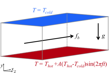
Figure 1: Schematic illustration of the temporally modulated mix convection channel.

We explore the dynamics of mixed convection within a three-dimensional (3-D) channel of dimensions $L\times H\times W$, as illustrated in figure 1. Here, $L$ is the length, $H$ is the height and $W$ is the width of the simulation domain, $x$ denotes the streamwise direction, $y$ denotes the wall-normal direction and $z$ denotes the spanwise direction. The computational domain size is chosen as $2\pi h\times 2h\times\pi h$ to ensure the spanwise domain size is close to the minimal spanwise size required to achieve developed turbulence in mixed convection simulations (Pirozzoli et al., 2017). Here, $h=H/2$ is the half-height of the channel. Periodic boundary conditions for velocity and temperature are applied in the streamwise and spanwise directions to exploit statistical homogeneity. In the wall-normal direction, no-slip velocity boundary conditions are imposed on the top and bottom walls of the channel. The grid size distribution is symmetric about the mid-plane, with cell sizes increasing geometrically from the wall to the bulk using a geometric progression. Specifically, the cell size for the $i$th grid $\Delta y_{i}$ can be defined as $\Delta y_{i}=\Delta y_{\text{wall}}q^{i-1}$ (for $i=1,2,\cdots,M$), where $\Delta y_{\text{wall}}$ is the starting cell size, $q$ is the common ratio of the geometric progression, and $M$ is the number of cells in the half-channel. The expansion ratio $r$ of the cell size, defined as the ratio of the end cell size $\Delta y_{\text{bulk}}$ to the starting cell size $\Delta y_{\text{wall}}$, is expressed as $r=\Delta y_{\text{bulk}}/\Delta y_{\text{wall}}$. This gives $q=r^{1/(M-1)}$ and $\Delta y_{\text{wall}}=h(1-q)/(1-q^{M})$. We set $r=8$ for $Ra=10^{6}$, $r=5$ for $Ra=10^{7}$ and $10^{8}$ in the simulations. We referenced the grid setup used by Pirozzoli et al. (2017), which is based on the resolution requirements for pure buoyant flow (Shishkina et al., 2010) and pure channel flow (Bernardini et al., 2014). We performed an a posteriori validation for all simulation cases, ensuring that the grid size in each coordinate direction is less than three Kolmogorov units in all cases.

$Ra$	$Ri_{b}$	$f^{*}$	$Re_{\tau}$ (bottom/top)	$Re_{\tau}$ difference	$N_{x}\times N_{y}\times N_{z}$
$10^{6}$	0.0445	unmodulated	$175.05/176.03$	$0.56\%$	$192\times 156\times 96$
$10^{6}$	0.0445	1	$175.44/175.75$	$0.18\%$	$192\times 156\times 96$
$10^{6}$	0.0445	0.1	$169.02/179.75$	$6.35\%$	$192\times 156\times 96$
$10^{6}$	0.0445	0.01	$167.82/178.10$	$6.13\%$	$192\times 156\times 96$
$10^{7}$	0.445	unmodulated	$197.90/198.71$	$0.41\%$	$384\times 256\times 192$
$10^{7}$	0.445	1	$197.50/197.35$	$0.08\%$	$384\times 256\times 192$
$10^{7}$	0.445	0.1	$202.33/212.50$	$5.03\%$	$384\times 256\times 192$
$10^{7}$	0.445	0.01	$187.11/214.35$	$14.56\%$	$384\times 256\times 192$
$10^{8}$	4.45	unmodulated	$272.43/273.01$	$0.21\%$	$384\times 256\times 192$
$10^{8}$	4.45	1	$270.25/272.21$	$0.73\%$	$384\times 256\times 192$
$10^{8}$	4.45	0.1	$266.75/286.46$	$7.39\%$	$384\times 256\times 192$
$10^{8}$	4.45	0.01	$251.19/295.31$	$15.56\%$	$384\times 256\times 192$

Table 1: Numerical details on flow quantities. The columns from left to right indicate the following: Rayleigh number $Ra$, bulk Richardson number $Ri_{b}$, wall-temperature modulation frequency $f^{*}$, friction Reynolds number $Re_{\tau}$ at the bottom and top wall, respectively, and their relative differences due to asymmetric boundary conditions, grid number $N_{x}\times N_{y}\times N_{z}$.

For the temperature boundary condition, the top wall is maintained at a constant low temperature of $T_{\text{top}}=T_{\text{cold}}$, while the bottom wall is subjected to a sinusoidal modulation $T_{\text{bottom}}=T_{\text{hot}}+A(T_{\text{hot}}-T_{\text{cold}})\sin(2\pi ft)$. Here, $A$ is the modulation amplitude, $f$ is the modulation frequency, and $t$ is time. We define the phase angle of the modulation as $\phi=2\pi ft$, and this phase angle $\phi$ will be used to describe the temporal progression of the modulation. The modulation amplitude is fixed as $A=2$, resulting in a temperature difference $\Delta_{T}^{*}=\left(T_{\text{bottom}}-T_{\text{top}}\right)/\left(T_{\text{hot}}-T_{\text{cold}}\right)=1+2\sin\left(2\pi ft\right)$, covering the regimes of unstable stratification ($\Delta_{T}>0$), neutral stratification ($\Delta_{T}=0$), and stable stratification ($\Delta_{T}<0$). Previously, Yang et al. (2020) fixed the modulation amplitude as $A=1$ in RB convection, which did not explore the stable stratification cases because $A=1$ leads to $\Delta_{T}\geq 0$ . We adopt the buoyancy timescale $t_{f}=\sqrt{H/(g\beta\Delta_{T})}$ to non-dimensionalize the modulation period $T_{\text{period}}$ as $T_{\text{period}}^{*}=T_{\text{period}}/t_{f}$ (Yang et al., 2020). We set the dimensionless modulation frequency $f^{*}$ in the range $0.01\leq f^{*}=1/T_{\text{period}}^{*}=t_{f}/T_{\text{period}}\leq 1$. Another approach is to adopt the bulk convective timescale $t_{b}=H/u_{b}$ to non-dimensionalize the modulation period as $T_{\text{period}}^{*}=T_{\text{period}}/t_{b}$. In this case, the modulation frequency is given by $f^{*}_{b}=t_{b}/T_{\text{period}}=f^{*}t_{b}/t_{f}$, leading to $f^{*}_{b}=\sqrt{Ri_{b}}f^{*}$. Because the wall temperature modulation changes the buoyancy within the flow system, we will focus on discussing $f^{*}$ in the following analysis.

To determine the Rayleigh number, the time-averaged temperature difference $\langle{\Delta_{T}}\rangle_{t}=T_{\text{hot}}-T_{\text{cold}}$ is adopted as $Ra=g\beta\langle{\Delta_{T}}\rangle_{t}H^{3}/(\nu\alpha)$, and the Rayleigh number is in the range of $10^{6}\leq Ra\leq 10^{8}$. We fix the Prandtl number as $Pr=0.71$ for the working fluid of air. The bulk Reynolds number is $Re_{b}=10^{3.75}\approx 5623$, and the corresponding friction Reynolds number $Re_{\tau}=u_{\tau}h/\nu$ is also provided in table 1, where $u_{\tau}=\sqrt{\langle{\tau_{w}}\rangle/\rho}$ is the friction velocity associated with the mean wall shear stress $\langle{\tau_{w}}\rangle$. We are particularly interested in the mixed convection regime, such that the Richardson number is in the range of $0.0445\leq Ri_{b}\leq 4.45$. A list of the bulk flow parameters obtained from all the simulations conducted in this study is provided in table 1, and their relevance to atmospheric currents in desert regions is discussed in Appendix B.

3 Results and discussion

3.1 Instantaneous flow and heat transfer features

In figure 2, we show snapshots of iso-surfaces of the $Q$-criterion, colored by the local temperature $T^{*}$, and the corresponding video can be viewed in supplementary movie 1. The $Q$-criterion visualizes vortices where the magnitude of vorticity $\mathbf{\Omega}=[\nabla\mathbf{u}-(\nabla\mathbf{u})^{T}]/2$ exceeds the magnitude of the strain rate $\mathbf{S}=[\nabla\mathbf{u}+(\nabla\mathbf{u})^{T}]/2$, making it an effective tool for illustrating vortical structures (Hunt et al., 1988). At a higher modulation frequency of $f^{*}=1$ (see figures 2a,c,e,g), the vortex structure are concentrated near the wall and appear relatively unchanged across different phase angle. At a lower modulation frequency of $f^{*}=0.01$ (see figures 2b,d,f,h), the effect of temporal modulation on wall temperature is evident, and the vortex structure exhibits a pronounced temporal evolution. Specifically, an increased number of structures are identified at $\phi=\pi/2$ and $\phi=\pi$, carried by hot fluids. An interesting observation is that when the wall temperature modulation leads to a stable condition (see figure 2h), the vortices near the bottom wall almost disappear. The absence of vortex interaction implies that the turbulent flow near the bottom wall is significantly weakened, although vortices still emerge and turbulent flow remains active on the top wall. The slower modulation frequency allows for the development of diverse flow structures and temperature distributions at each phase, indicating the fluid’s ability to adapt to each state of the heating and cooling cycles. In contrast, rapid modulation does not give the fluid enough time to significantly rearrange its structure within one modulation cycle, resulting in a consistent pattern regardless of the phase angle.

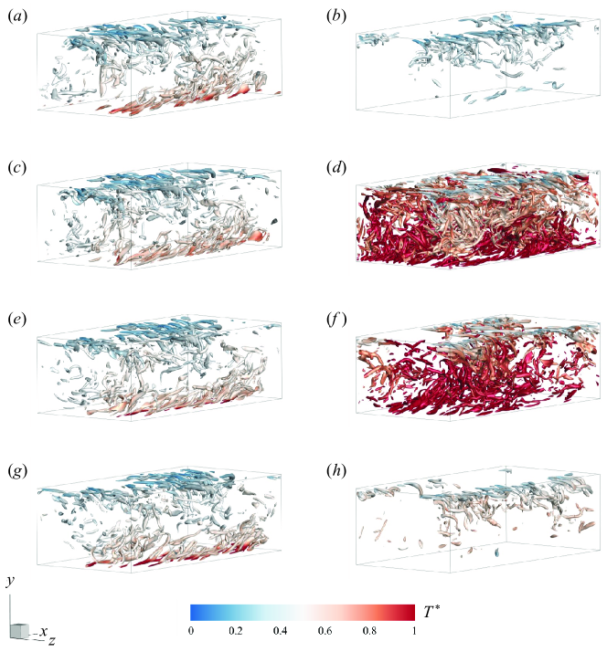
Figure 2: Typical instantaneous iso-surfaces of the $Q$-criterion, $Q^{*}=\left(\|\mathbf{\Omega}^{*}\|^{2}-\|\mathbf{S}^{*}\|^{2}\right)/2=15$ colored by the local temperature $T^{*}$, at phase angle (a,b) $\phi=0$, (c,d) $\phi=\pi/2$, (e,f) $\phi=\pi$, (g,h) $\phi=3\pi/2$, with frequency (a,c,e,g) $f^{*}=1$, (b,d,f,h) $f^{*}=0.01$, for $Ra=10^{7}$ and $Re_{b}\approx 5623$.

We show the instantaneous velocity component $v^{*}$ at the channel center plane ($y=h$) in figure 3, corresponding to the instantaneous state presented in figure 2. In convective flow, rising fluids are warmer, and falling fluids are colder; thus, we do not show the corresponding temperature field $T^{*}$ at this plane. However, we have verified that the correlation coefficient between $v^{*}$ and $T^{*}$ is larger than 0.47. At a Rayleigh number of $Ra=10^{7}$ and a bulk Reynolds number of $Re_{b}\approx 5623$, with a fixed Prandtl number of $Pr=0.71$, the corresponding Richardson number is $Ri_{b}=0.45$. At this intermediate Richardson number, the shear-driven and buoyancy-driven turbulence production rates are nearly balanced. The flow exhibits rolls pointing in the streamwise direction, with a strong meandering behavior due to the wavy instability of the rolls. This overall trend is similar to that reported by Pirozzoli et al. (2017). In addition, we found that at a higher modulation frequency of $f^{*}=1$ (see figures 3a,c,e,g), the pair of counter-rotating rolls within the flow domain remains relatively stable in strength. The stability of these rolls demonstrates the flow’s resilience against high-frequency thermal perturbations, suggesting an inherent inertia in the thermal field that resists rapid changes. However, at a lower modulation frequency of $f^{*}=0.01$ (see figures 3b,d,f,h), the strength of the roll varies with the phase angle. Specifically, the rolls are stronger during the heating phase ($T_{\text{bottom}}>T_{\text{hot}}$); it is much weaker, or even disappear, during the cooling phase ($T_{\text{bottom}}<T_{\text{hot}}$).

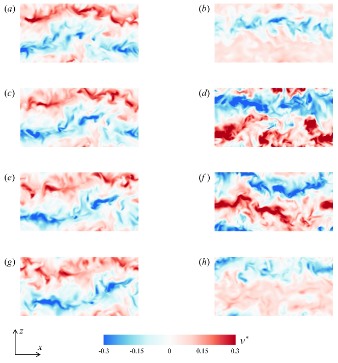
Figure 3: Typical instantaneous velocity component $v^{*}$ at channel center plane ($y=h$) at phase angle (a,b) $\phi=0$, (c,d) $\phi=\pi/2$, (e,f) $\phi=\pi$, (g,h) $\phi=3\pi/2$, with frequency (a,c,e,g) $f^{*}=1$, (b,d,f,h) $f^{*}=0.01$, for $Ra=10^{7}$ and $Re_{b}\approx 5623$.

We show the temperature field $T^{*}$ in the cross-stream plane, which complements the velocity contours at the channel center plane shown in figure 3. During the heating phase, we observe frequent hot plume emissions near the bottom wall, becoming more pronounced after the wall temperature cycle reaches its peak (see figures 4e,f). In contrast, during the cooling phase (see figures 4g,h), plume emissions from the bottom wall are absent due to stable stratification, resulting in the weakening of buoyancy forces. In this stable stratification, internal gravity waves separate the bottom cold part and the top hot part (Zonta et al., 2022). We also observe the effect of modulation frequency on temperature evolution. At a higher frequency of $f^{*}=1$, the upward- and downward-travelling plumes detaching from the boundary layers are almost unaffected by the phase angle, explaining the relatively stable pair of counter-rotating rolls found in figures 3(a,c,e,g). At a lower frequency of $f^{*}=0.01$, the slower frequency allows the temperature to respond to changes in the thermal boundaries and adapt to each state of the modulation cycle (see figures 4b,d,f,h). During the heating phase, hot rising plumes deeply penetrate into the bulk region of the channel. During the cooling phase, a stably stratified layer forms near the bottom wall, acting as a thermal blanket. The overall behaviour mirrors the dynamics observed in atmospheric flow (Dupont & Patton, 2022). After sunrise, the ground heats up, destabilizing atmospheric conditions and forming a mixed layer with a relatively uniform temperature profile due to turbulent mixing. After sunset, the ground cools down more rapidly than the air above it, forming a stable boundary layer close to the surface. This layer sits beneath the remnants of the daytime mixed layer, where turbulence gradually decays in the absence of additional production mechanisms.

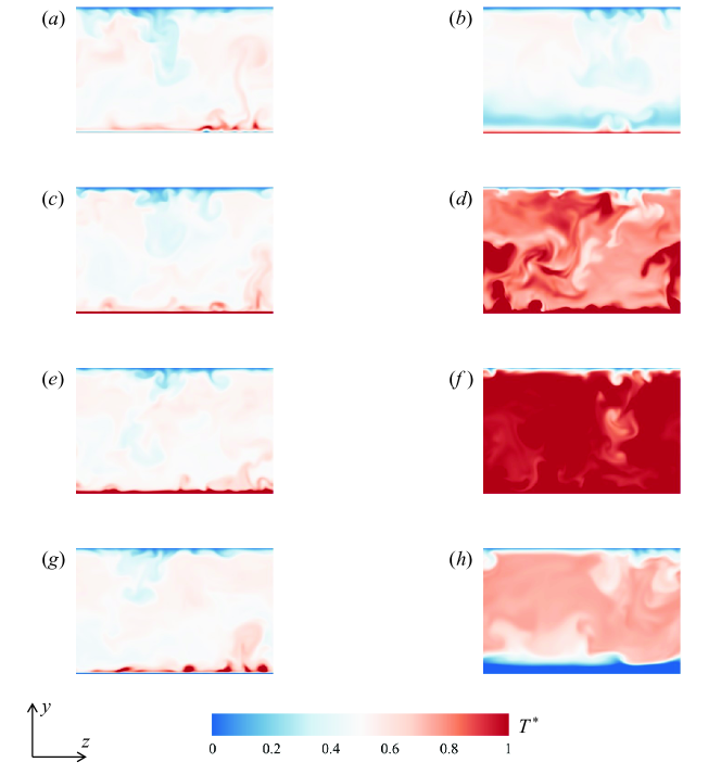
Figure 4: Typical instantaneous temperature $T^{*}$ in cross-stream plane at phase angle (a,b) $\phi=0$, (c,d) $\phi=\pi/2$, (e,f) $\phi=\pi$, (g,h) $\phi=3\pi/2$, with frequency (a,c,e,g) $f^{*}=1$, (b,d,f,h) $f^{*}=0.01$, for $Ra=10^{7}$ and $Re_{b}\approx 5623$.

To examine the influence of wall temperature modulation on local heat transfer properties, we show slices of vertical convective heat flux $v^{*}\delta T^{*}$ in figure 5, corresponding to the instantaneous state presented in figure 2. Here, the temperature fluctuation is defined as $\delta T^{*}=T^{*}-0.5$. At a higher frequency of $f^{*}=1$ (see figures 5a,c,e,g), positive values of vertical heat flux predominantly appear within the channel, while negative values occur near both the top and bottom walls. This counter-gradient heat transfer is attributed to sweeps of hotter fluid toward the bottom wall and colder fluid toward the top wall. In contrast, at a lower frequency of $f^{*}=0.01$ (see figures 5b,d,f,h), there is a strong counter-gradient heat flux in the bulk region of the channel, driven by the bulk dynamics of rolls, similar to the mechanism in RB convection (Gasteuil et al., 2007; Huang & Zhou, 2013). Detached plumes move with the streamwise-oriented roll, and after reaching the opposite wall, some plumes retain thermal energy and remain hotter or colder than their surroundings. They continue moving with the rolls, resulting in the falling of hot fluid or the rising of cold fluid, thus generating negative vertical heat flux.

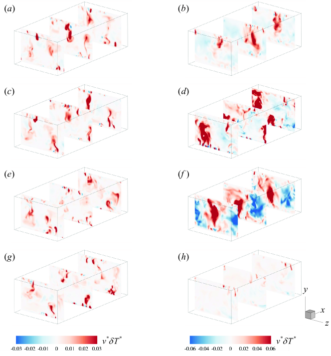
Figure 5: Typical instantaneous vertical convective heat flux $v^{*}\delta T^{*}$ at phase angle (a,b) $\phi$ = 0, (c,d) $\phi$ = $\pi$/2, (e,f) $\phi$ = $\pi$, (g,h) $\phi$ = 3$\pi$/2, with frequency (a,c,e,g) $f^{*}=1$, (b,d,f,h) $f^{*}=0.01$, for $Ra=10^{7}$ and $Re_{b}\approx 5623$.

We further show the instantaneous streamwise velocity component $u^{*}$ at a near-wall station of $y=0.05h$ in figure 6. At a higher modulation frequency of $f^{*}=1$ (see figures 6a,c,e,g), near-wall streaks are observed even in the presence of strong buoyancy. These streaks are often associated with vigorous momentum transfer and robust turbulence production. However, at a lower modulation frequency of $f^{*}=0.01$ (see figures 6b,d,f,h), during the cooling phase, which leads to stable stratification of the fluid, the near-wall burst-sweep process is completely disrupted (see figure 6h). This disruption ceases turbulence production and shows tendencies of relaminarization near the bottom wall. During the heating phase, which leads to unstable stratification, the near-wall streaks appear again.

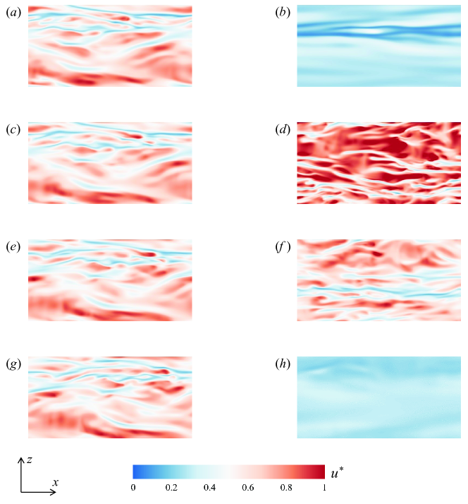
Figure 6: Typical instantaneous velocity component $u^{*}$ at near-wall station ($y=0.05h$) at phase angle (a,b) $\phi=0$, (c,d) $\phi=\pi/2$, (e,f) $\phi=\pi$, (g,h) $\phi=3\pi/2$, with frequency (a,c,e,g) $f^{*}=1$, (b,d,f,h) $f^{*}=0.01$, for $Ra=10^{7}$ and $Re_{b}\approx 5623$.

To extract the large-scale coherent flow structures, we perform proper orthogonal decomposition (POD) on the turbulent dataset (Berkooz et al., 1993). The POD has been widely employed to study the dynamics of large-scale circulation in convection cells (Podvin & Sergent, 2015; Castillo-Castellanos et al., 2019; Soucasse et al., 2019; Xu et al., 2021). Specifically, the spatiotemporal flow velocity field $\mathbf{u}(\textbf{x},t)$ is decomposed into a superposition of empirical orthogonal eigenfunctions $\mathbf{\phi}_{i}(\mathbf{x})$ and their scalar amplitudes $a_{i}(t)$ as

$$\mathbf{u}(\mathbf{x},t)=\sum_{i=1}^{\infty}a_{i}(t)\mathbf{\phi}_{i}(\mathbf{x}).$$ (9)

Here, $\mathbf{u}(\mathbf{x},t)=[u(\mathbf{x},t),v(\mathbf{x},t),w(\mathbf{x},t)]^{T}$ represents the vector field with components $u$, $v$, and $w$. $\mathbf{\phi}_{i}(\mathbf{x})=[\phi_{i}^{u}(\mathbf{x}),\phi_{i}^{v}(\mathbf{x}),\phi_{i}^{w}(\mathbf{x})]^{T}$ represents the spatial eigenfunctions (i.e. the POD modes), and $a_{i}(t)$ are the temporal coefficients representing the time-dependent amplitudes of the corresponding modes. We used at least 900 snapshots to adequately capture the flow structure, ensuring the dominant modes are representative. At parameters of $Ra=10^{7}$ and $Re_{b}\approx 5623$ (i.e. the corresponding $Ri_{b}=0.445$), we have the most energetic POD mode corresponds to the streamwise unidirectional shear flow with parallel streamlines pointing along the $x$-direction. Then, in figures 7(a,b,c), we present the second most energetic POD modes, which are essentially the dominant mode for the fluctuation velocity field. Regardless of the temporal modulation frequency of the bottom wall temperature, streamwise-oriented rolls that full filled the whole channel height are observed. We also examined the time series of mode amplitudes $a_{i}(t)$ and studied the relationship between wall temperature $T_{\text{bottom}}\left(t\right)=T_{\text{hot}}+2(T_{\text{hot}}-T_{\text{cold}})\sin(2\pi ft)$ and the second POD mode amplitude $a_{2}(t)$ by calculating their cross-correlation functions as

$$R_{T_{\text{bottom}},a_{2}}\left(\tau\right)=\frac{\left\langle\left[T_{\text{bottom}}\left(t+\tau\right)-\left\langle T_{\text{bottom}}\right\rangle\right]\left[a_{2}(t)-\left\langle a_{2}\right\rangle\right]\right\rangle}{\sigma_{T_{\text{bottom}}}\sigma_{a_{2}}}$$ (10)

where $\sigma_{T_{\text{bottom}}}$ and $\sigma_{a_{2}}$ are the standard deviation of $T_{\text{bottom}}$ and ${a_{2}}$, respectively. As shown in figures 7(d,e,f), at higher modulation frequency of $f^{*}=1$ and $f^{*}=0.1$, $T_{\text{bottom}}$ are uncorrelated with ${a_{2}}$, indicating that the large-scale rolls are not influenced by changes in wall temperature. However, at a lower modulation frequency of $f^{*}=0.01$, we observe a strong correlation between $T_{\text{bottom}}$ and $a_{2}$, implying that the strength of the large-scale rolls is significantly affected by temperature modulation on the wall. These large-scale rolls are a recognized structural characteristic of atmospheric boundary layers, present in scenarios with mean streamwise flow and exhibiting overall streamwise helical patterns. These patterns are responsible for transporting warmer air towards the capping inversion and cooler air towards the ground (Jayaraman & Brasseur, 2021).

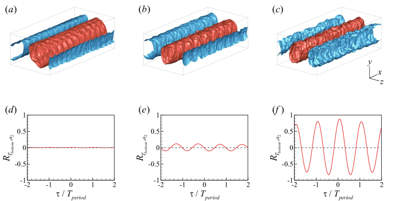
Figure 7: (a-c) The second most energetic POD modes, visualizations of isosurfaces of vertical velocity $v$ (red color represents $v>0$ and blue color represents $v<0$), and (d-f) the cross-correlation functions between bottom wall temperature $T_{\text{bottom}}(t)$ and POD mode amplitudes $a_{2}(t)$ as a function of dimensionless lag time $\tau/T_{\text{period}}$, at modulation frequency of (a,d) $f^{*}=1$, (b,e) $f^{*}=0.1$, (c,f) $f^{*}=0.01$, for $Ra=10^{7}$ and $Re_{b}\approx 5623$.

We then computed the energy content of the $i$th POD mode $\lambda_{i}$. In figure 8, we show the spectra of $\lambda_{i}$, where each value of $\lambda_{i}$ is normalized by the total energy $\sum\lambda_{i}$. At $Ra=10^{7}$, the energy content of the first POD mode $\lambda_{1}$ dominates, accounting for over 95% of the total energy and representing the mean flow (streamwise unidirectional shear flow). The energy content of the second and third POD modes $\lambda_{2}$ and $\lambda_{3}$, each contributes approximately 0.1-0.6% of the total energy. At a higher Rayleigh number of $Ra=10^{8}$, with the same bulk Reynolds number of $Re_{b}\approx 5623$, the energy contained in the first mode reduces to about 80% due to the enhanced effect of buoyancy, while the second and third modes each contribute around 2% of the total energy. These results indicate that both the second and third modes play a role in capturing the flow dynamics, suggesting that the flow morphology is influenced by the interaction between these modes rather than by a single dominant structure.

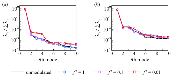
Figure 8: The energy contained in each mode, for (a) $Ra=10^{7}$ and (b) $Ra=10^{8}$.

Due to the periodicity in the wall boundary conditions, the streamwise-oriented rolls are non-stationary and continually move along the spanwise direction. To illustrate this, we quantitatively describe the movement of the rolls by tracking their center. Because the axes of these rolls align with the streamwise and do not exhibit the complex motion seen in RB convection (Vogt et al., 2018; Li et al., 2022; Teimurazov et al., 2023), we can track their edges by identifying locations where the vertical velocity component is minimal or maximal. The center of each roll is then determined by calculating the arithmetic mean of these points. The POD analysis reveals that not only the second most energetic POD modes but also higher POD modes can represent these rolls. For example, at $Ra=10^{7}$, $Re_{b}\approx 5623$, and $f^{*}=0.1$, both the second and third POD modes correspond to streamwise-oriented rolls, albeit offset along the spanwise direction. Thus, we use both the second and third POD modes to recover the streamwise-oriented roll at $f^{*}=0.1$. Figure 9(a) shows the instantaneous recovered flow field at $x=L/2$, representing a pair of counter-rotating streamwise-oriented rolls. Here, we mark the edges and center of one roll to demonstrate the effectiveness of our approach to tracking the roll motion. When the roll center exits one side of the domain, we account for the domain’s periodicity by wrapping its position to the opposite side, resulting in a continuous trajectory. In figure 9(b), we plot the time series of the center of this roll along the spanwise direction. The results suggest that the streamwise-oriented roll moves along the spanwise direction, occasionally appearing to exit from one side of the domain and re-enter from the other.

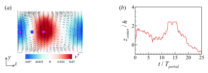
Figure 9: (a) Typical instantaneous flow field recovered using the second and third POD mode at $Ra=10^{7}$, $Re_{b}\approx 5623$ and $f^{*}=0.1$. The contour represents the vertical velocity component, and the arrow represents the velocity field of recovered velocity components. The magenta diamonds mark the edges the rolls, the blue circles mark the roll center. (b) The time series of the position of roll center.

A smaller domain may restrict the formation of large structures due to the imposed periodic boundary conditions and limited spatial extent (Stevens et al., 2024), thus we conducted additional simulations in a larger domain ($4\pi h\times 2h\times 2\pi h$). In this expanded domain, at $Ra=10^{7}$ and $Re_{b}\approx 5623$ (i.e. the corresponding $Ri_{b}=0.445$), we observed two pairs of counter-rotating straight rolls (see figure 10a), which align with expectations based on domain scaling. In other words, doubling the horizontal extent resulted in two roll pairs, compared to one pair in the smaller domain. We then examined the second POD modes in this large domain at $Ra=10^{8}$ and $Re_{b}\approx 5623$ (i.e. the corresponding $Ri_{b}=4.45$). As shown in figure 10(b), the isosurfaces reveal variations in the vertical velocity, with alternating regions of upward (positive) and downward (negative) flow. The higher Rayleigh number induces stronger buoyancy forces and increased thermal driving, which leads to the breakdown of coherent rolls into smaller, more chaotic structures. While these structures remain somewhat aligned in the streamwise direction, they appear increasingly fragmented, indicating a transition toward a more convection-dominated state. Accordingly, we refer to these structures at $Ra=10^{8}$ as fragmented streamwise-oriented rolls.

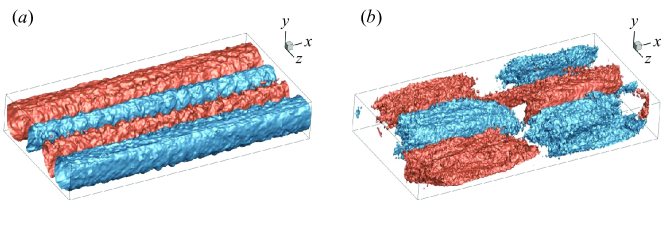
Figure 10: The second POD mode in a domain size of $4\pi h\times 2h\times 2\pi h$, visualizations of isosurfaces of vertical velocity (red color represents $v>0$ and blue color represents $v<0$) at (a) $Ra=10^{7}$, (b) $Ra=10^{8}$, with $f^{*}=0.1$.

3.2 Long-time averaged statistics

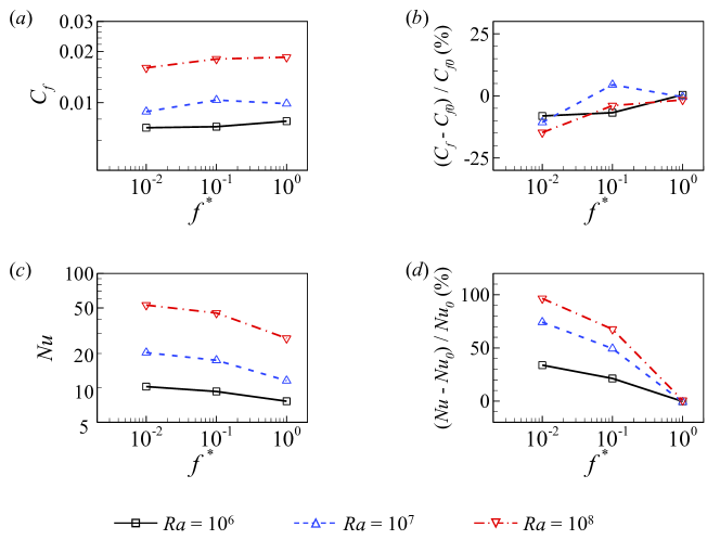
Figure 11: (a) Friction coefficient, (b) values of $C_{f}/C_{f0}-1$, (c) Nusselt number, (d) values of $Nu/Nu_{0}-1$, as functions of $f^{*}$ for various $Ra$. Here, $C_{f0}$ and $Nu_{0}$ are the friction coefficient and Nusselt numbers without wall temperature modulation, respectively.

To study changes induced on the mean flow and temperature by the wall temperature modulation, we now focus on the long-time averaged statistics. In figure 11, we present statistics of aerodynamic drag and heat transfer as a function of modulation frequency for various Rayleigh numbers, which is a topic of interest in meteorology and engineering (Yerragolam et al., 2022, 2024). In figure 11(a), we examine the aerodynamic drag in terms of friction coefficients ($C_{f}$) at the bottom wall, which is calculated as $C_{f}=2\langle\tau_{w}\rangle/(\rho u_{b}^{2})$. The increased drag due to the emission of plumes in thermal field is consistent with that reported by Scagliarini et al. (2015); Pirozzoli et al. (2017); Howland et al. (2024). With wall temperature modulation, we observe that aerodynamic drag is not very sensitive to the wall temperature modulation frequency. Figure 11(b) further visualizes the relative changes of $C_{f}$ with wall temperature modulation, showing that the variation in $C_{f}$ is less than 15%. In figure 11(c), we examine the heat transfer efficiency in terms of the Nusselt number ($Nu$), which is calculated as $Nu=\sqrt{RaPr/Ri_{b}}\left\langle v^{*}T^{*}\right\rangle_{V,t}+1$. Here, $\langle\cdots\rangle_{V,t}$ denotes the ensemble average over the whole channel and over the time. The $Nu$ at the highest modulation frequency is the same as that without wall temperature modulation. With the decrease in modulation frequency, we observe enhanced heat transfer efficiency for all Rayleigh numbers. Previously, in pure RB convection, Yang et al. (2020) reported a regime where the modulation is too fast to affect $Nu$, a regime where $Nu$ increases with decreasing $f^{*}$, and a regime where $Nu$ decreases with further decreasing $f^{*}$. Our results in mixed PRB convection cover the first two regimes reported in pure RB convection, yet we did not further explore slower frequency due to the high computational cost in the 3-D simulation. Figure 11(d) further visualizes that among the three Rayleigh numbers, the $Ra=10^{8}$ results in the largest magnitude of heat transfer efficiency, up to 96%. At high Rayleigh numbers, convective patterns are more vigorous, and wall temperature modulation has a more disruptive effect. Higher frequencies likely cause more frequent disturbances in the boundary layers, reducing heat transfer efficiency by breaking up coherent thermal plumes.

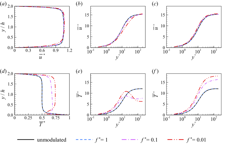
Figure 12: Mean profiles of (a-c) streamwise velocity and (d-f) temperature: (a,d) along the whole channel height, (b,e) along the bottom half-height, (c,f) along the top half-height, for $Ra=10^{7}$ and $Re_{b}\approx 5623$.

In figure 12, we show the mean profiles for streamwise velocity and temperature across the channel height to illustrate the effects of wall temperature modulation on the mean flow. We denote the mean velocity and mean temperature by an overbar, and the fluctuating quantities by a prime, thus we have $u=\overline{u}+u^{\prime}$ and $T=\overline{T}+T^{\prime}$. Consistent with our observations on flow organization, these mean profiles are similar between scenarios without wall temperature modulation and those with the highest modulation frequency ($f^{*}=1$). For the mean streamwise velocity profile, it is symmetric about the mid-plane $y=h$ at the highest frequency of $f^{*}=1$; however, slight asymmetry is observed at lower frequencies of $f^{*}=0.1$ and 0.01 (see figure 12a). This asymmetrical is also evident from table 1, which shows the relative differences in friction Reynolds numbers. To highlight the modulation effect in the near-wall regions, we replot the velocity data using wall scaling in figures 12(b) and 12(c). Here, the superscript ’+’ indicates normalization using the kinematic viscosity $\nu$ and the friction velocity $u_{\tau}$ in wall units. The distances from the walls are then given by $y^{+}=yu_{\tau}/\nu$. We can see that at lower frequencies, the average streamwise velocity $\overline{u}^{+}=\overline{u}/u_{\tau}$ decreases near the bottom wall (see figure 12b) and increases near the top wall (see figure 12c). As for the mean temperature profile, at $f^{*}=1$, the temperature decreases monotonically from the bottom wall, stabilizing at a constant value of the arithmetic mean temperature $T^{*}=0.5$ in the bulk region, and is antisymmetric about the mid-plane (see figure 12d). This pattern recovers the canonical RB convection profile. However, at $f^{*}=0.1$ and 0.01, deviations from the profiles without wall modulation are evident. The temperature first decreases and then increases near the bottom wall, until it reaches a plateau in the bulk region. Similar to findings in the RB convection (Yang et al., 2020), our results suggest that at lower modulation frequencies, the bulk temperature increases compared to cases without wall temperature modulation. We also replot the temperature data using wall scaling, as shown in figures 12(e) and 12($f$). For a straightforward comparison between the heating and cooling sides, we calculate the average temperature as $\overline{T}^{+}=\left|\overline{T}-\langle T_{\text{wall}}\rangle\right|/T_{\tau}$. Here, $\langle T_{\text{wall}}\rangle$ is the mean temperature at either the bottom wall or top wall, and the friction temperature $T_{\tau}=Q/u_{\tau}$ is used to normalize the average temperature, where $Q$ is total vertical heat flux, calculated as $Q=(\alpha\Delta_{T}/H)Nu$. At $f^{*}=0.1$ and 0.01, we observe a peak in the $\overline{T}^{+}$ profile at $y^{+}\approx 17$ (see figure 12e) due to the formation of thermal Stokes layers by the oscillatory wall temperature (Yang et al., 2020); however, such a peak is absent at a higher frequency of $f^{*}=1$, as well as near the top wall where the wall temperature is constant (see figure 12$f$).

To examine the influence of wall-temperature modulation on turbulence quantities, in figure 13, we present the root-mean-square fluctuation of velocity components and temperature along the lower half-height of the channel. The peak of the root-mean-square (r.m.s.) streamwise velocity profile consistently occurs at $y^{+}\approx 15$ (see figure 13a), where turbulent eddies are most active, similar to observations in turbulent channel flow without convection (Moser et al., 1999). The wall-normal velocity fluctuation increases throughout the half-channel height due to wall temperature modulation, becoming comparable to or even larger than the streamwise component (see figure 13b). These fluctuations, sensitive to buoyancy effects, suggest that lower-frequency thermal modulations enhance buoyancy-driven turbulence. The spanwise velocity fluctuation also increases in the near-wall region with wall temperature modulation (see figure 13c). This increase in wall-normal and spanwise velocity fluctuation implies that fluid columns rising from the bottom wall activate cross-stream eddies near the wall. As for the r.m.s. of the temperature (see figure 13d), lower frequency wall temperature modulations ($f^{*}=0.01$) yield higher peaks in temperature fluctuations near the wall, indicating a more unstable thermal boundary layer with larger eddies under slower temperature modulation. In contrast, higher frequencies ($f^{*}=1$) appear to stabilize the thermal boundary layer, leading to less pronounced temperature fluctuations.

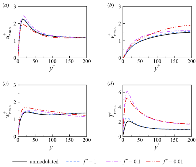
Figure 13: Root-mean-square fluctuation of (a) streamwise velocity, (b) wall-normal velocity, (c) spanwise velocity, and (d) temperature along the bottom half-height of the channel, for $Ra=10^{7}$ and $Re_{b}\approx 5623$.

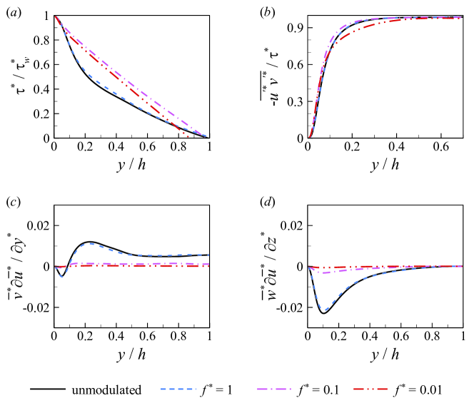
Figure 14: Profile of (a) total shear stress, (b) percentage of Reynolds stress to the total shear stress, (c) convective term component $\overline{v}^{*}\partial\overline{u}^{*}/\partial y$, (d) convective term component $\overline{w}^{*}\partial\overline{u}^{*}/\partial z$ along the channel half-height, for $Ra=10^{7}$ and $Re_{b}\approx 5623$.

Wall temperature modulation also influences the wall-normal behavior of momentum flux. Because the mean flow is predominantly in the axial direction for our investigated flow parameters, we plot the distribution of shear stress $\tau(y)=\rho\nu d\overline{u}/dy-\overline{u^{\prime}v^{\prime}}$ in terms of dimensionless function $\tau^{*}/\tau_{w}^{*}$ across the lower half of the channel height (from $y=0$ to $y=h$) in figure 14(a), where $\tau_{w}^{*}$ is the dimensionless wall shear stress. In figure 14(b), we further show the contribution of Reynolds stress $-\overline{u^{\prime*}v^{\prime*}}$ to the total shear stress $\tau^{*}$. At a higher frequency of $f^{*}=1$, the total shear stress exhibits a non-linear distribution, whereas at lower frequencies of $f^{*}=0.1$ and $f^{*}=0.01$, it decreases linearly along the channel’s half-height. The linear distribution of $\tau^{*}/\tau_{w}^{*}$ at lower frequencies resembles the shear stress profile observed in a pure turbulent channel without convection. To further explain the deviation from linear total shear stress at higher frequencies, we examine the mean-momentum equation along the streamwise direction within the mixed convection channel

$$\begin{split}\overline{u}^{*}\frac{\partial\bar{u}^{*}}{\partial x^{*}}+\overline{v}^{*}\frac{\partial\bar{u}^{*}}{\partial y^{*}}+\overline{w}^{*}\frac{\partial\bar{u}^{*}}{\partial z^{*}}&=-\frac{\partial\overline{P}^{*}}{\partial x^{*}}+\frac{1}{Re_{b}}\left(\frac{\partial^{2}\overline{u}^{*}}{\partial x^{*2}}+\frac{\partial^{2}\overline{u}^{*}}{\partial y^{*2}}+\frac{\partial^{2}\overline{u}^{*}}{\partial z^{*2}}\right)\\ &-\left(\frac{\partial\overline{u^{\prime*}u^{\prime*}}}{\partial x^{*}}+\frac{\partial\overline{u^{\prime*}v^{\prime*}}}{\partial y^{*}}+\frac{\partial\overline{u^{\prime*}w^{\prime*}}}{\partial z^{*}}\right)+\overline{f_{b}}^{*}\\ \end{split}$$ (11)

Here, the terms for $\partial\left(\cdot\right)/\partial x^{*}$ and $\partial^{2}(\cdot)/\partial x^{*2}$ are near zero in the fully developed region, where velocity statistics no longer vary with the streamwise direction, as confirmed by our DNS results. Due to the detachment of thermal plumes from the wall and their horizontal spreading, the homogeneous condition along the spanwise direction may be violated, making the terms $\partial(\cdot)/\partial z^{*}$ and $\partial^{2}(\cdot)/\partial z^{*2}$ non-zero near the wall. However, we numerically verified (not shown here for simplicity) that the magnitudes of $(1/Re_{b})\partial^{2}\overline{u}^{*}/\partial z^{*2}$ and $\partial\overline{u^{\prime*}w^{\prime*}}/\partial z^{*}$ are three orders smaller than the other terms, so they can be neglected. Thus, (11) can be rewritten as

$$\frac{\partial}{\partial y^{*}}\left(\frac{1}{Re_{b}}\frac{\partial\overline{u}^{*}}{\partial y^{*}}-\overline{u^{\prime*}v^{\prime*}}\right)=\overline{v}^{*}\frac{\partial\overline{u}^{*}}{\partial y^{*}}+\overline{w}^{*}\frac{\partial\overline{u}^{*}}{\partial z^{*}}-\overline{f_{b}}^{*}\ \ \ \Rightarrow\ \ \ \frac{d\tau^{*}}{dy^{*}}=\overline{v^{*}}\frac{\partial\overline{u}^{*}}{\partial y^{*}}+\overline{w}^{*}\frac{\partial\overline{u}^{*}}{\partial z^{*}}-\overline{f_{b}}^{*}$$ (12)

At a higher frequency of $f^{*}=1$, the convection effects are more pronounced for the mean flow, resulting in finite values for the components $\overline{v}^{*}\partial\overline{u}^{*}/\partial y^{*}$ and $\overline{w}^{*}\partial\overline{u}^{*}/\partial z^{*}$, as shown in figures 14(c) and 14(d). At lower frequencies of $f^{*}=0.1$ and $0.01$, the convection effects are substantially reduced for the mean flow, making $\overline{v}^{*}\partial\overline{u}^{*}/\partial y^{*}$ and $\overline{w}^{*}\partial\overline{u}^{*}/\partial z^{*}$ close to zero, restoring conditions similar to a pure turbulent channel. This reduced convection for the mean flow is mainly attributed to the formation of a stably stratified layer near the bottom wall, which acts as a thermal blanket, effectively suppressing buoyancy forces.

Figure 15: Profiles of (a,b) flux Richardson number and (c,d) turbulent Prandlt number, along the (a,c) the bottom half channel and (b,d) the top half channel, respectively, for $Ra=10^{7}$ and $Re_{b}\approx 5623$.

We quantify the local relative dynamic importance of buoyancy compared to friction using the flux Richardson number, which is calculated as (Pirozzoli et al., 2017)

$$Ri_{f}=\frac{-\beta g\overline{\nu^{\prime}T^{\prime}}}{\overline{u^{\prime}\nu^{\prime}}d\bar{u}/dy}$$ (13)

In figures 15(a) and 15(b), we plot $Ri_{f}$ along the bottom and top halves of the channel height, respectively. Regardless of the wall modulation frequency, the near-wall region ($y\leq 0.2h$) is dominated by shear. However, as we move farther away from the wall, convection begins to emerge and eventually dominates in the bulk region. We also quantify the ratio of turbulent momentum to thermal diffusivity via the turbulent Prandlt number $Pr_{t}$, which is frequently used in modeling turbulent heat transfer. For simple shear flows, the Reynolds analogy suggests that $Pr_{t}$ is of the order of unity (Kays, 1994). Using DNS results, we can calculate $Pr_{t}$ as

$$Pr_{t}=\frac{\nu_{t}}{\alpha_{t}}=\frac{\overline{u^{\prime}v^{\prime}}}{\overline{v^{\prime}T^{\prime}}}\frac{d\overline{T}/dy}{d\overline{u}/dy}$$ (14)

Here, $\nu_{t}$ is turbulent viscosity and $\alpha_{t}$ is the thermal eddy diffusivity. On the bottom side (see figure 15c), at a high frequency of $f^{*}=1$ and the unmodulated case, $Pr_{t}$ is close to unity in the near-wall region; however, at lower modulation frequencies, $Pr_{t}$ deviates from unity significantly because the temperature is more efficiently transported compared to momentum. On the top side (see figure 15d), $Pr_{t}$ approximates unity near the wall, yet it exhibits a large variation in the bulk region. These features of the $Pr_{t}$ distribution present challenges in turbulence modeling, where a constant value is often assumed.

3.3 Phase-averaged statistics

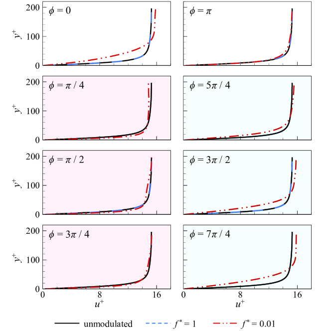
Figure 16: Phase-averaged streamwise velocity profiles $\left\langle u^{+}(y)\right\rangle_{\phi}$ along the bottom half-height for $Ra=10^{7}$ and $Re_{b}\approx 5623$. For the case without wall temperature modulation, we present the long-time averaged profiles to guide the eye.

Because the wall temperature modulation inherently induces unsteady flow and temperature evolution, we now focus on the phase-averaged statistics. We will present the variability of the physical quantities during different phases of the flow cycle and how they are affected by the wall temperature modulation. In the following, we denote with the brackets $\left\langle\cdot\right\rangle$ all quantities that have been phase averaged. We first calculate the phase-averaged streamwise velocity $\left\langle u^{+}(\mathbf{x})\right\rangle_{\phi}$ and plot its profile $\left\langle u^{+}\left(y\right)\right\rangle_{\phi}=\left[\int_{0}^{L}\int_{0}^{W}\left\langle u^{+}\left(\mathbf{x}\right)\right\rangle_{\phi}dzdx\right]/\left(LW\right)$ along the bottom half of the channel height, as shown in figure 16. At a high frequency of $f^{*}=1$, the flow maintains a velocity profile consistent with that under constant wall temperature. However, at a lower frequency of $f^{*}=0.01$, the velocity profiles deviate from those without wall-temperature modulation, particularly in the near-wall region where the thermal boundary layer causes variations in the velocity gradients. An interesting observation is that during the cooling phase (e.g. at a phase angle of $\phi=5\pi/4,3\pi/2,7\pi/4$), the streamwise velocity near the wall significantly decreases. This occurs because the turbulence intensity near the bottom wall is greatly weakened by the cooling. As a result, the reduced turbulence results in lower surface drag on the fluid above, leading to an acceleration of the flow and a higher plateau away from the wall compared to the constant wall temperature condition. This trend aligns with the dynamics of the nocturnal low-level jet in atmospheric flow. At night, surface cooling creates stable conditions and temperature inversions, which suppress turbulence near the ground. This suppression reduces surface drag and allows for the formation of nocturnal jets characterized by higher wind speeds above the cooled surface layer. Understanding the behavior of nocturnal jets is crucial for sandstorms, air pollution, wind energy utilization, and aviation safety (Liu et al., 2014).

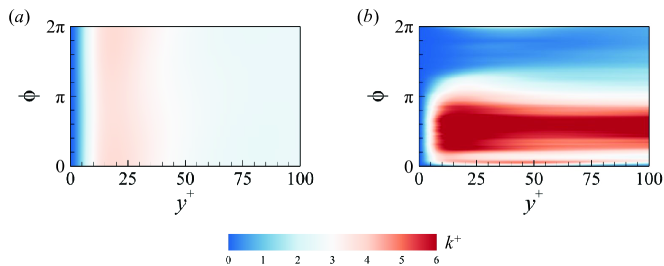
Figure 17: Space-phase diagrams of turbulent kinetic energy along the bottom half-height for $Ra=10^{7}$ and $Re_{b}\approx 5623$: (a) $f^{*}=1$, (b) $f^{*}=0.01$.

The behavior of velocity distribution can be further understood by studying the phase-averaged turbulent kinetic energy (TKE) as $k^{+}=\langle{u_{i}^{\prime+}u_{i}^{\prime+}}\rangle_{\phi}/2$. Here, the subscript $i$ is a dummy index, and the superscript (^′) denotes the fluctuation part of an instantaneous flow variable. In figure 17, we show the space-phase diagram of turbulence intensities. At a high frequency of $f^{*}=1$ (see figure 17a), we can infer that the perturbation is relatively intense in the region $10\leq y^{+}\leq 40$ across different phases, and such consistent TKE leads to phase-averaged velocity profiles that are insensitive to phase variations. At a low frequency of $f^{*}=0.01$ (see figure 17b), there is phase-dependent variation in TKE diagrams, and turbulence intensity is strengthened and reduced alternately in one cycle. During heating phases, the flow behaves as unstable stratification, and TKE exhibits significant peaks in the range of $y^{+}\geq 10$; during cooling phases, the flow behaves similarly to stable stratification, TKE decreases to almost zero, and turbulence intensities are suppressed. Such reduced TKE results in lower velocity close to the wall and higher velocity aloft, as previously observed in figure 16. We examine the phase-averaged TKE equation of incompressible mixed convection, which is written as

$$\frac{\partial k^{+}}{\partial t^{+}}+\langle u_{j}^{+}\rangle_{\phi}\partial_{j^{+}}k^{+} =\underbrace{-\langle u_{i}^{\prime+}u_{j}^{\prime+}\rangle_{\phi}\partial_{j^{+}}\langle u_{i}^{+}\rangle_{\phi}}_{\langle P\rangle}$$ (15)

$$\quad\underbrace{-\partial_{j^{+}}\langle P^{\prime+}u_{j}^{\prime+}\rangle_{\phi}}_{\langle\Pi\rangle}\underbrace{-\frac{1}{2}\partial_{j^{+}}\langle u_{i}^{\prime+}u_{i}^{\prime+}u_{j}^{\prime+}\rangle_{\phi}}_{\langle T\rangle}+\underbrace{\partial_{j^{+}}\partial_{j^{+}}k^{+}}_{\langle D\rangle}$$

$$\quad\underbrace{-\langle(\partial_{j^{+}}u_{i}^{\prime+})^{2}\rangle_{\phi}}_{\langle\varepsilon\rangle}+\underbrace{\frac{Ra}{Pr(2Re_{\tau})^{3}}\langle T^{\prime*}v^{\prime+}\rangle_{\phi}}_{\langle B\rangle}$$

In the above, the terms $\langle P\rangle$ and $\langle B\rangle$ represent the production by shear and buoyancy, respectively; the terms $\langle\Pi\rangle$, $\langle T\rangle$, $\langle D\rangle$ represent turbulent diffusion by pressure-velocity fluctuations, velocity fluctuations, viscous diffusion, respectively; the term $\langle\varepsilon\rangle$ represents dissipation. In figure 18, we show the TKE budgets for $Ra=10^{7}$, $Re_{b}\approx 5623$, and $f^{*}=0.01$. The shear-induced and buoyancy-induced TKE productions are strongly influenced by the wall temperature modulation in both amplitude and peak position. Specifically, during the heating phase (e.g. at a phase angle of $\phi=\pi/4,\pi/2,3\pi/4$), the TKE production is dominated by shear in the near-wall region, while it is dominated by buoyancy in the bulk region. During the cooling phase (e.g. at a phase angle of $\phi=5\pi/4,3\pi/2,7\pi/4$), the TKE productions are all near zero along the whole channel height. For other terms of the budget, including the velocity-pressure gradient, the viscous diffusion, and the turbulent transport, the in-cycle variation is also evident during the heating phase in the near-wall region but shows minor variation during the cooling phase (see the insets in figure 18).

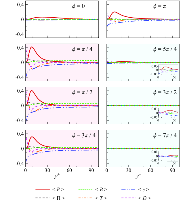
Figure 18: Phase-averaged turbulent kinetic energy budgets along the bottom half-height for $Ra=10^{7}$, $Re_{b}\approx 5623$ and $f^{*}=0.01$.

We then analyze the phase-averaged temperature $\left\langle T^{*}\left(\mathbf{x}\right)\right\rangle_{\phi}$ , and plot its profile $\left\langle T^{*}\left(y\right)\right\rangle_{\phi}=\left[\int_{0}^{L}\int_{0}^{W}\left\langle T^{*}\left(\mathbf{x}\right)\right\rangle_{\phi}dzdx\right]/\left(LW\right)$ along the bottom half channel height, as shown in figure 19. At a high frequency of $f^{*}=1$, the temperature profiles deviate from those without wall-temperature modulation only in the region of $y<0.1h$. Farther away from the wall, the influence of the modulation is limited. At a lower frequency of $f^{*}=0.01$, both the near-wall and bulk temperatures are influenced by the modulation. During the heating phase (e.g. at a phase angle of $\phi=\pi/4,\pi/2,3\pi/4$), the temperature decreases upward in the boundary layer, resulting in an unstably stratified flow. During the cooling phase (e.g. at a phase angle of $\phi=5\pi/4,3\pi/2,7\pi/4$), the temperature increases upward in the boundary layer, forming a statistically stable boundary layer. This stabilization suppresses turbulence and reduces mixing, leading to the formation of a residual layer above the stable boundary layer that retains the thermal stratification from the previous cycle. In meteorology, this residual layer is analogous to the one that retains the adiabatic lapse rate from the previous day, as described by Stull (2015).

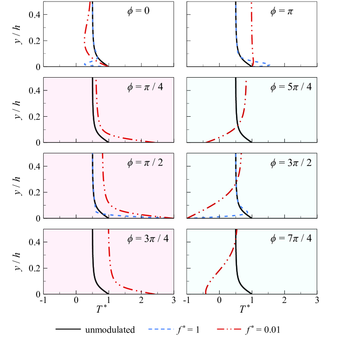
Figure 19: Phase-averaged temperature profiles $\left\langle T^{*}(y)\right\rangle_{\phi}$ along the bottom half channel height for $Ra=10^{7}$ and $Re_{b}\approx 5623$.

Heat accumulates within the boundary layer during the heating phase and is lost during the cooling phase, making temperature profiles dependent on the accumulated heating or cooling. In figure 20, we plot the phase-averaged dimensionless heat flux, represented by the Nusselt number at the bottom wall as $Nu_{\text{bottom}}=-\langle\partial T^{*}/\partial y^{*}\rangle_{\text{bottom},t}$. Here, $\langle\cdots\rangle_{\text{bottom},t}$ denotes the ensemble average over the bottom wall and over the time. At a high frequency of $f^{*}=1$ (see figure 20a), the phase-averaged $Nu_{\text{bottom}}$ exhibits substantial oscillation amplitude. This occurs because high modulation frequency causes rapid changes in thermal conditions, temporarily enhancing convective heat transfer. However, significant peaks and valleys may require robust control mechanisms to manage these rapid changes without causing fatigue due to thermal stress, thereby adding complexity to the system device components in applied thermal engineering applications. As the modulation frequency decreases (see figures 20b and 20c), the oscillation amplitude of $Nu_{\text{bottom}}$ decreases, indicating more stable heat transfer with smaller deviations from the baseline. This is ideal for applications requiring consistent thermal management without significant fluctuations. On the other hand, the long-time averaged values of Nusselt numbers generally increase as the modulation frequency decreases: $Nu$ is 11.58 at $f^{*}=1$ while $Nu$ is 20.36 at $f^{*}=0.01$ (marked by the dash lines in figure 20). These results suggest that the average $Nu$ might not fully capture the extreme fluctuations, which are critical for predicting and optimizing heat transfer in various engineering applications.

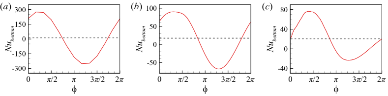
Figure 20: Phase-averaged dimensionless heat flux in terms of Nusselt number at the bottom wall, (a) $f^{*}=1$, (b) $f^{*}=0.1$, (c) $f^{*}=0.01$, for $Ra=10^{7}$ and $Re_{b}\approx 5623$. The dash lines represent long-time averaged values of $Nu$ at various modulation frequencies.

In addition, we observe the asymmetry in the Nusselt number $Nu_{\text{bottom}}$ during the heating and cooling phases at low modulation frequencies. At low frequencies (e.g. $f^{*}=0.01$), the system experiences extended periods of heating and cooling, allowing distinct thermal and flow structures to develop in each phase. The fluid’s thermal inertia causes a delayed response in heat transfer: while the heating phase rapidly amplifies convection, the cooling phase is moderated by the residual thermal energy in the fluid. Specifically, during the heating phase, as the bottom wall temperature increases and buoyancy forces enhance, the upward convective currents accelerate rapidly. The increasing temperature gradient thins the thermal boundary layer, reducing thermal resistance and enhancing heat transfer efficiency. As a result, $Nu_{\text{bottom}}$ rises quickly, forming higher but narrower peaks above the average value. During the cooling phase, as the bottom wall temperature decreases and buoyancy forces weaken, the established convective motions persist due to the fluid’s inertia. The decreasing temperature gradient thickens the thermal boundary layer, increasing thermal resistance and slowing down heat transfer. This results in a more gradual reduction in $Nu_{\text{bottom}}$, producing lower but wider regions below the average value.

Finally, we differentiate between the oscillatory flow induced by wall-temperature modulation and the fluctuating fields. To that end, we adopt the phase decomposition method, which has been widely applied in the investigation of turbulent flows subjected to periodic forcing, such as channel turbulence or turbulent boundary layers with oscillating walls (Choi, 2002; Ricco et al., 2012; Ebadi et al., 2019), oscillatory or pulsating pipe flows (Manna et al., 2015; Jelly et al., 2020), and the oscillatory thermal turbulence (Wu et al., 2021, 2022). The key idea of phase decomposition method is to split the instantaneous field $\mathbb{F}{\left(\mathbf{x},t\right)}$ into the long-time averaged quantity $\overline{\mathbb{F}}(\mathbf{x})$, the oscillatory quantity $\tilde{\mathbb{F}}{\left(\mathbf{x},t_{n}\right)}$, and the turbulent fluctuation $\mathbb{F}^{\prime}(\mathbf{x},t)$, which is written as

$$\mathbb{F}(\mathbf{x},t)=\overline{\mathbb{F}}(\mathbf{x})+\overset{\sim}{\operatorname*{\mathbb{F}}}(\mathbf{x},t_{n})+\mathbb{F}^{\prime}(\mathbf{x},t)$$ (16)

Here, the oscillatory quantity is calculated as $\widetilde{\mathbb{F}}(\mathbf{x},t_{n})=\left\langle\mathbb{F}(\mathbf{x})\right\rangle_{\phi}-\overline{\mathbb{F}}(\mathbf{x})$. We divide the oscillating period $T_{\text{period}}$ into $M$ evenly spaced intervals, and $t_{n}=(n-1)T_{\text{period}}/M$ is the time corresponding to the phase angle of $\phi_{n}=2(n-1)\pi/M$. Previously, Yang et al. (2020) investigated the thermal Stokes problem in pure RB convection, where the temperature oscillated in modulated pure RB convection. The oscillatory temperature can be obtained analytically as $\tilde{T}(y,t_{n})=Ae^{-y^{*}/\lambda_{s}^{*}}\sin(\phi_{n}-y^{*}/\lambda_{s}^{*})$, with the Stokes thermal boundary layer thickness being $\lambda_{s}^{*}=\pi^{-1/2}f^{*-1/2}Ra^{-1/4}Pr^{-1/4}$. Here, the term $Ae^{-y^{*}/\lambda_{s}^{*}}$ indicates that the effect of the oscillating boundary temperature decays exponentially with distance from the boundary, while the term $\sin(\phi_{n}-y^{*}/\lambda_{s}^{*})$ indicates a phase lag of $y^{*}/\lambda_{s}^{*}$ in the temperature oscillation as we move away from the boundary.

We compare the analytical and numerical solutions of oscillatory temperature in mixed PRB convection, as shown in figure 21. A good agreement is observed at a high frequency of $f^{*}=1$ (see figure 21a); however, deviations occur at lower frequencies of $f^{*}=0.1$ and 0.01 (see figures 21b and 21c). These discrepancies may be attributed to two factors. First, the penetration depth of the temperature disturbance induced by the oscillating wall temperature is inversely proportional to the modulation frequency. Consequently, at lower frequencies, the temperature disturbance penetrates deeper into the flow, potentially exceeding the thermal boundary layer thickness. Within the thermal boundary, we can assume a heat conduction profile for the temperature, which aligns with the analytical model (Yang et al., 2020). Outside the thermal boundary, the effects of convection become significant, causing deviations from the analytical predictions. In figure 21, we mark the depth where the oscillating temperature’s amplitude drops to 1% of its maximum value (approximately equal to 4.6$\lambda_{s}^{*}$), as well as the thermal boundary layer thickness (determined from the peak positions of the r.m.s. temperature profile). The results show that at a higher frequency of $f^{*}=1$, the oscillating temperature penetration depth is of the same order of magnitude as the thermal boundary layer thickness. However, at a lower frequency of $f^{*}=0.01$, the penetration depth is an order of magnitude thicker than the thermal boundary layer thickness.

Moreover, our simulations included an imposed pressure gradient (achieved via an equivalent body force), which introduces mean shear that affects the velocity field throughout the fluid domain, including within the thermal boundary layer. This shear enhances convective transport parallel to the wall, modifying the temperature profile. A critical factor here is the ratio of the thermal diffusion timescale to the convective timescale induced by the mean shear. We denote the thermal diffusion timescale $t_{\text{diff}}$ as the characteristics time it takes for heat to diffuse across the penetration depth $\lambda_{s}$, with $t_{\text{diff}}\propto\lambda_{s}^{2}/\alpha$ (where $\alpha$ is the thermal diffusivity). We also denote the convective timescale $t_{\text{conv}}$ as the characteristics time it takes for fluid particles to be advected by the mean shear across the penetration depth, with $t_{\text{conv}}\propto\lambda_{s}/U$ (where $U$ is the characteristic velocity of the Poiseuille flow near the wall). Comparing these timescales, we have the ratio $t_{\text{diff}}/t_{\text{conv}}\propto f^{*-1/2}$. As the modulation frequency $f^{*}$ decreases, the thermal diffusion timescale $t_{\text{diff}}$ becomes larger compared to the convective timescale $t_{\text{conv}}$, indicating that convection becomes more significant within the penetration depth. This increased significance of convection, driven by the mean shear, contributes to the discrepancies between the analytical and simulation results.

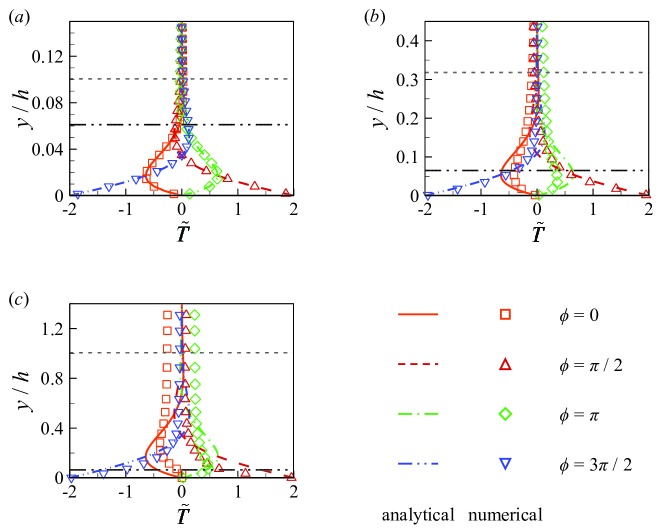
Figure 21: Comparison of oscillatory temperature from analytical and numerical solutions, at (a) $f^{*}=1$, (b) $f^{*}=0.1$, (c) $f^{*}=0.01$, for $Ra=10^{7}$ and $Re_{b}\approx 5623$. The gray dashed lines show the depth where the oscillating temperature’s amplitude drops to 1% of its maximum value, and the black dash-dotted lines show the thermal boundary layer thickness.

4 Conclusion

In this work, we have performed DNS of mixed convection in turbulent PRB channels with sinusoidal wall temperature modulation. High-frequency wall temperature oscillations resulted in a relatively unchanged flow structure, while low-frequency oscillations caused the flow structures to adapt over time, forming stable stratified layers during the cooling phase. Using the POD method, we identified the most energetic mode as a dominant streamwise unidirectional shear flow. Regardless of modulation frequency, streamwise-oriented large-scale rolls appeared as higher POD modes. Streamwise-oriented rolls were strongly correlated with wall temperature variations at lower frequencies, indicating a significant influence on roll strength. We also tracked the movements of roll centres, showing that large-scale rolls exhibit non-stationary behaviour influenced by the periodic boundary conditions of the computational domain. In addition, vertical convective heat flux analysis revealed counter-gradient heat transfer driven by thermal plumes at high frequencies and by bulk roll dynamics at low frequencies.

We then explored the impact of wall temperature modulation on long-time averaged statistics of mean flow and temperature. The friction coefficient showed less than a 15% variation with modulation frequency. In contrast, the Nusselt number increased as the frequency decreased, particularly at higher Rayleigh numbers, with an increase up to 96%. High-frequency modulation minimally affected the mean profiles of streamwise velocity and temperature. However, lower frequencies increased the velocity near the top wall and decreased it near the bottom wall, and the temperature profile deviated from that of canonical RB convection. Total shear stress varied non-linearly at high frequencies but linearly at lower frequencies, resembling the behavior of a pure turbulent channel without convection. This difference arises because high-frequency modulation enhances convective effects near the wall, while lower frequencies reduce these effects by forming a stable stratified layer.

Finally, we analyzed phase-averaged statistics to understand variability during different phases of the flow cycle. At high modulation frequency, the phase-averaged streamwise velocity profile remained stable. However, at low frequencies, the velocity decreased near the wall and increased away from it due to weakened turbulence. The TKE profiles were consistently high near the wall at high frequency, but they were lower during the cooling phases at low frequency. The TKE budget analysis revealed that shear dominated TKE production near the wall during heating, while buoyancy dominated in the bulk region; both TKE productions were nearly zero during cooling. High modulation frequency confined temperature deviations to the region near the wall, whereas lower frequency affected temperatures both near the wall and in the bulk region. During heating, temperature decreased upward in the boundary layer, leading to unstable stratification. During cooling, temperature increased upward, creating a stable boundary layer that suppressed turbulence and formed a residual layer. Phase-averaged Nusselt numbers showed substantial oscillation amplitude at high frequency due to rapid thermal changes, while oscillations decreased with lower frequency, leading to more stable and efficient heat transfer.

Overall, our study highlights the complex interplay between wall temperature modulation frequency and flow dynamics in mixed convection, providing insights relevant to meteorology and heat transfer engineering applications. However, we acknowledge that the limited spanwise domain size may inhibit the development of the largest coherent structures and alter the flow morphology compared to larger domains representative of atmospheric flows. Furthermore, the limited range of flow parameters restricts our ability to fully mimic the extreme flow conditions in atmospheric currents. Therefore, caution should be exercised when generalizing these results to larger-scale flows, such as those in the atmospheric boundary layer. Future studies with larger computational domains and higher Rayleigh and Reynolds numbers could provide additional insights into scale-dependent behaviors and further validate the applicability of our conclusions to real-world atmospheric flows.

[Supplementary data]Supplementary material and movies are available at
https://doi.org/10.1017/jfm.2024…

[Funding]This work was supported by the National Natural Science Foundation of China (NSFC) through Grants No. 12272311, No. 12125204, and No. 12388101, the Young Elite Scientists Sponsorship Program by CAST (2023QNRC001), and the 111 project of China (Project No. B17037).

[Declaration of interests]The authors report no conflict of interest.

[Author ORCIDs]Ao Xu, https://orcid.org/0000-0003-0648-2701; Heng-Dong Xi, https://orcid.org/0000-0002-2999-2694

Appendix A Cross-validation of solvers against benchmark data.

Here, we validate the consistency of results among the benchmark data from Pirozzoli et al. (2017), our in-house solver based on the lattice Boltzmann method (LBM), and the OpenFOAM solver based on the finite volume method (FVM). As shown in figure 22, we compare flow quantities including the mean profiles of temperature and streamwise velocity, as well as the root-mean-square fluctuations of temperature, streamwise velocity, wall-normal velocity, and spanwise velocity along the bottom half-height of the channel. The results demonstrate good agreement among all three datasets, confirming the accuracy and reliability of our simulation results. Furthermore, table 2 provides a detailed quantitative comparison of flow quantities. The numerical comparison shows minimal deviations, with discrepancies remaining within acceptable ranges for turbulent simulations, further reinforcing the consistency of the results.

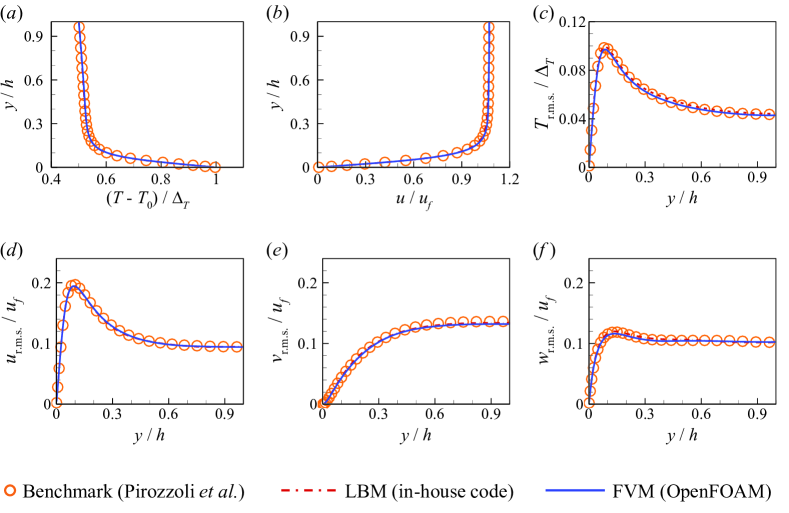
Figure 22: Comparison of data from Pirozzoli et al. (2017) as benchmark, our in house code based on LBM, and OpenFOAM code based on FVM. Mean profiles of (a) temperature and (b) streamwise velocity, mean-square fluctuation of (c) temperature, (d) streamwise velocity, (e) wall-normal velocity, and (f) spanwise velocity along the bottom half-height of the channel for $Re_{b}\approx 3162$, $Ra=10^{7}$, and $Pr=1$.

Flow database	$Re_{\tau}$	$Nu$	$C_{f}$	$N_{x}$	$N_{y}$	$N_{z}$
Benchmark (Pirozzoli et al.)	142.59	11.622	$1.62\times 10^{-2}$	256	256	128
LBM (in-house code)	142.08	11.713	$1.62\times 10^{-2}$	420	210	210
FVM (OpenFOAM)	141.62	11.616	$1.60\times 10^{-2}$	256	256	128

Table 2: Quantitative comparison of flow quantities among benchmark, LBM and FVM solvers. The columns from left to right indicate the following: flow database, friction Reynolds number ($Re_{\tau}$), Nusselt number ($Nu$), skin friction coefficient ($C_{f}$), grid number in the streamwise, wall-normal, and spanwise directions ($N_{x}$, $N_{y}$, $N_{z}$).

Appendix B Parameter estimation for desert atmospheric currents.

We consider typical desert atmospheric conditions, where the characteristic height $H$ is approximately 1000 m, representing the atmospheric boundary layer height. For air at a mean temperature $T_{\text{mean}}=300$ K, the thermal expansion coefficient is $\beta=3.36\times 10^{-3}$ K^-1, the kinematic viscosity is $\nu=1.57\times 10^{-5}$ m²/s, and the thermal diffusivity is $\alpha=2.22\times 10^{-5}$ m²/s. The temperature difference across the atmospheric boundary layer can be $\Delta_{T}\approx 20$ K or more. The gravitational acceleration is $g=9.8$ m/s².

i) Modulation Amplitude. In desert regions, surface temperatures fluctuate significantly due to strong solar heating during the day and rapid radiative cooling at night, leading to both unstable and stable stratification over 24 hours. To mimic this, we vary the bottom wall temperature as $T_{\text{bottom}}=T_{\text{hot}}+A(T_{\text{hot}}-T_{\text{cold}})\sin(2\pi ft)$, representing a sinusoidal variation around $T_{\text{hot}}=[(T_{\text{bottom}})_{\min}+(T_{\text{bottom}})_{\max}]/2$. Data from the moderate resolution imaging spectroradiometer observations (Sharifnezhadazizi et al., 2019) indicate that land surface temperatures in the Shara Desert range between $(T_{\text{bottom}})_{\min}=280$ K and $(T_{\text{bottom}})_{\max}=310$ K, suggesting an average bottom wall temperature of $T_{\text{hot}}=295$ K. Above the atmospheric boundary layer, diurnal cycles are absent, so the top wall temperature is fixed as $T_{\text{top}}=T_{\text{cold}}$. Assuming a lapse rate-adjusted temperature at the top boundary, we estimate $T_{\text{top}}=T_{\text{cold}}\approx T_{\text{hot}}–6.5$ K/km $\times$ 1 km $\approx 288.5$ K. Thus, $A=\left[(T_{\text{bottom}})_{\max}-T_{\text{hot}}\right]/(T_{\text{hot}}-T_{\text{cold}})\approx 2.3$, closely matching our chosen value of $A=2$.

ii) Modulation Frequency. The diurnal frequency associated with the day-night cycle is relatively low. On Earth, a 24-hour diurnal period corresponds to a frequency of approximately $f_{\text{diurnal}}=1/(24\times 3600\ \text{s})\approx 1.16\times 10^{-5}$ Hz. To relate this to our dimensionless frequency $f^{*}$, we estimate the free-fall time scale as $t_{f}=\sqrt{H/(g\beta\Delta_{T})}\approx 39$ s, yielding a dimensionless diurnal frequency of $f^{*}=f_{\text{diurnal}}t_{f}\approx 4.5\times 10^{-4}$. This value is two orders of magnitude smaller than the lower limit of our study (i.e. $f^{*}=0.01$). Exploring lower frequencies would require significantly more computational resources to ensure the convergence of phase-averaged statistics over extended simulation times.

iii) Prandlt number. The Prandlt number characterizes the thermophysical properties of a fluid and is defined as $Pr=\nu/\alpha$. It quantifies the ratio of viscous diffusion to thermal diffusivity. For air, we have $Pr\approx 0.71$, which closely matches our settings.

iv) Rayleigh number. The Rayleigh number characterizes the intensity of convection in a fluid system and is defined as $Ra=g\beta\Delta_{T}H^{3}/(\nu\alpha)$. It quantifies the balance between buoyancy-driven forces and diffusive transport (viscous and thermal diffusion). For typical desert atmospheric conditions, we have $Ra\approx 2\times 10^{18}$.

v) Friction Reynolds number. The friction Reynolds number characterizes turbulent shear near the wall and is defined as $Re_{\tau}=u_{\tau}H/\nu$. To estimate the friction velocity $u_{\tau}$, we use the logarithmic wind profile $U(z)=u_{\tau}/\kappa\ln(z/z_{0})$, where $\kappa\approx 0.4$ is the von Kármán constant, and $z_{0}$ is the roughness length. For desert surfaces, we estimate $z_{0}=0.01$ m. During sandstorms, wind speeds reach 13.9 m/s or higher (i.e. Level 7 on the Beaufort scale, measured at $z=10$ m), resulting in a friction velocity of $u_{\tau}\approx 0.8$ m/s, giving $Re_{\tau}\approx 5\times 10^{7}$.

vi) Bulk Reynolds number. The bulk Reynolds number represents the ratio of inertial forces to viscous forces in the flow, considering the average motion of the fluid across the entire flow domain, and is defined as $Re_{b}=u_{b}H/\nu$. Using the logarithmic wind profile, we obtain the mean bulk velocity $u_{b}$ as $\left(\int_{z_{0}}^{H}U(z)dz\right)/H\approx u_{\tau}/\kappa\left[\ln(H)-1-\ln(z_{0})\right]\approx 21$ m/s, leading to $Re_{b}\approx 1\times 10^{9}$. The corresponding bulk Richardson number is $Ri_{b}=Ra/(Re_{b}^{2}Pr)\sim O(1)$, suggesting that global buoyancy and shear effects are comparable.

These high Rayleigh and Reynolds numbers align with the expected intense turbulence and large-scale atmospheric motions, indicating an extreme flow condition. There remains a significant gap between current computational capabilities and the requirements for direct numerical simulation or large eddy simulation of sheared thermal turbulence under such extreme parameters.

References

- Ahlers et al. (2009) Ahlers, G., Grossmann, S. & Lohse, D. 2009 Heat transfer and large scale dynamics in turbulent Rayleigh-Bénard convection. Rev. Mod. Phys. 81 (2), 503–537.
- Andreotti et al. (2009) Andreotti, B., Fourriere, A., Ould-Kaddour, F., Murray, B. & Claudin, P. 2009 Giant aeolian dune size determined by the average depth of the atmospheric boundary layer. Nature 457 (7233), 1120–1123.
- Berkooz et al. (1993) Berkooz, G., Holmes, P. & Lumley, J. L. 1993 The proper orthogonal decomposition in the analysis of turbulent flows. Annu. Rev. Fluid Mech. 25 (1), 539–575.
- Bernardini et al. (2014) Bernardini, M., Pirozzoli, S. & Orlandi, P. 2014 Velocity statistics in turbulent channel flow up to . J. Fluid Mech. 742, 171–191.
- Blass et al. (2021) Blass, A., Tabak, P., Verzicco, R., Stevens, R.J.A.M. & Lohse, D. 2021 The effect of Prandtl number on turbulent sheared thermal convection. J. Fluid Mech. 910, A37.
- Blass et al. (2020) Blass, A., Zhu, X., Verzicco, R., Lohse, D. & Stevens, R.J.A.M. 2020 Flow organization and heat transfer in turbulent wall sheared thermal convection. J. Fluid Mech. 897, A22.
- Brown (1980) Brown, R. A. 1980 Longitudinal instabilities and secondary flows in the planetary boundary layer: A review. Rev. Geophys. 18 (3), 683–697.
- Castillo-Castellanos et al. (2019) Castillo-Castellanos, A., Sergent, A., Podvin, B. & Rossi, M. 2019 Cessation and reversals of large-scale structures in square Rayleigh–Bénard cells. J. Fluid Mech. 877, 922–954.
- Caulfield (2021) Caulfield, C. P. 2021 Layering, instabilities, and mixing in turbulent stratified flows. Annu. Rev. Fluid Mech. 53 (1), 113–145.
- Chen & Sreenivasan (2023) Chen, X. & Sreenivasan, K.R. 2023 Reynolds number asymptotics of wall-turbulence fluctuations. J. Fluid Mech. 976, A21.
- Chilla et al. (2012) Chilla, T., Evrard, E. & Schulz, C. 2012 On the territoriality of cross-border cooperation: “Institutional Mapping” in a multi-level context. Eur. Plan. Stud. 20 (6), 961–980.
- Choi (2002) Choi, K.-S. 2002 Near-wall structure of turbulent boundary layer with spanwise-wall oscillation. Phys. Fluids 14 (7), 2530–2542.
- Cossu (2022) Cossu, C. 2022 Onset of large-scale convection in wall-bounded turbulent shear flows. J. Fluid Mech. 945, A33.
- Dror et al. (2023) Dror, T., Koren, I., Liu, H. & Altaratz, O. 2023 Convective steady state in shallow cloud fields. Phys. Rev. Lett. 131 (13), 134201.
- Dupont & Patton (2022) Dupont, S. & Patton, E. G. 2022 On the influence of large-scale atmospheric motions on near-surface turbulence: Comparison between flows over low-roughness and tall vegetation canopies. Bound.-Layer Meteor. 184 (2), 195–230.
- Ebadi et al. (2019) Ebadi, A., White, C. M., Pond, I. & Dubief, Y. 2019 Mean dynamics and transition to turbulence in oscillatory channel flow. J. Fluid Mech. 880, 864–889.
- Garai et al. (2014) Garai, A., Kleissl, J. & Sarkar, S. 2014 Flow and heat transfer in convectively unstable turbulent channel flow with solid-wall heat conduction. J. Fluid Mech. 757, 57–81.
- Gasteuil et al. (2007) Gasteuil, Y., Shew, W. L., Gibert, M., Chillà, F., Castaing, B. & Pinton, J.-F. 2007 Lagrangian temperature, velocity, and local heat flux measurement in Rayleigh-Bénard convection. Phys. Rev. Lett. 99 (23), 234302.
- Graham & Floryan (2021) Graham, M. D. & Floryan, D. 2021 Exact coherent states and the nonlinear dynamics of wall-bounded turbulent flows. Annu. Rev. Fluid Mech. 53 (1), 227–253.
- Hanna (1969) Hanna, S. R. 1969 The formation of longitudinal sand dunes by large helical eddies in the atmosphere. J. Appl. Meteorol. Climatol. 8 (6), 874–883.
- Howland et al. (2024) Howland, C.J., Yerragolam, G.S., Verzicco, R. & Lohse, D. 2024 Turbulent mixed convection in vertical and horizontal channels. J. Fluid Mech. 998, A48.
- Huang & Zhou (2013) Huang, Y.-X. & Zhou, Q. 2013 Counter-gradient heat transport in two-dimensional turbulent Rayleigh–Bénard convection. J. Fluid Mech. 737, R3.
- Hunt et al. (1988) Hunt, J. C. R., Wray, A. A. & Moin, P. 1988 Eddies, streams, and convergence zones in turbulent flows. Studying Turbulence Using Numerical Simulation Databases, 2. Proceedings of the 1988 Summer Program .
- Iida & Kasagi (1997) Iida, O. & Kasagi, N. 1997 Direct numerical simulation of unstably stratified turbulent channel flow. ASME J. Heat Transf. 119 (1), 53–61.
- Jayaraman & Brasseur (2021) Jayaraman, B. & Brasseur, J. G. 2021 Transition in atmospheric boundary layer turbulence structure from neutral to convective, and large-scale rolls. J. Fluid Mech. 913, A42.
- Jelly et al. (2020) Jelly, T. O., Chin, R. C., Illingworth, S. J., Monty, J. P., Marusic, I. & Ooi, A. 2020 A direct comparison of pulsatile and non-pulsatile rough-wall turbulent pipe flow. J. Fluid Mech. 895, R3.
- Jiang et al. (2020) Jiang, H., Zhu, X., Wang, D., Huisman, S.G. & Sun, C. 2020 Supergravitational turbulent thermal convection. Sci. Adv. 6 (40), eabb8676.
- Jiménez (2012) Jiménez, J. 2012 Cascades in wall-bounded turbulence. Annu. Rev. Fluid Mech. 44 (1), 27–45.
- Jiménez (2013) Jiménez, J. 2013 Near-wall turbulence. Phys. Fluids 25 (10), 101302.
- Jin & Xia (2008) Jin, X.-L. & Xia, K.-Q. 2008 An experimental study of kicked thermal turbulence. J. Fluid Mech. 606, 133–151.
- Kays (1994) Kays, W. M. 1994 Turbulent Prandtl number. Where are we? ASME J. Heat Transf. 116 (2), 284–295.
- Kok et al. (2012) Kok, J. F., Parteli, E. J. R., Michaels, T. I. & Karam, D. B. 2012 The physics of wind-blown sand and dust. Rep. Prog. Phys. 75 (10), 106901.
- Komen et al. (2014) Komen, E., Shams, A., Camilo, L. & Koren, B. 2014 Quasi-DNS capabilities of OpenFOAM for different mesh types. Comput. Fluids 96, 87–104.
- Komen et al. (2017) Komen, E. M. J., Camilo, L. H., Shams, A., Geurts, B. J. & Koren, B. 2017 A quantification method for numerical dissipation in quasi-DNS and under-resolved DNS, and effects of numerical dissipation in quasi-DNS and under-resolved DNS of turbulent channel flows. J. Comput. Phys. 345, 565–595.
- Komen et al. (2023) Komen, E. M. J., Mathur, A., Roelofs, F., Merzari, E. & Tiselj, I. 2023 Status, perspectives, and added value of high fidelity simulations for safety and design. Nucl. Eng. Des. 401, 112082.
- Komori et al. (1982) Komori, S., Ueda, H., Ogino, F. & Mizushina, T. 1982 Turbulence structure in unstably-stratified open-channel flow. Phys. Fluids 25 (9), 1539–1546.
- Kooij et al. (2018) Kooij, G. L., Botchev, M. A., Frederix, E. M. A., Geurts, B. J., Horn, S., Lohse, D., van der Poel, E. P., Shishkina, O., Stevens, R.J.A.M. & Verzicco, R. 2018 Comparison of computational codes for direct numerical simulations of turbulent Rayleigh–Bénard convection. Comput. Fluids 166, 1–8.
- Li et al. (2022) Li, Y.-Z., Chen, X., Xu, A. & Xi, H.-D. 2022 Counter-flow orbiting of the vortex centre in turbulent thermal convection. J. Fluid Mech. 935, A19.
- Liu et al. (2014) Liu, H., He, M., Wang, B. & Zhang, Q. 2014 Advances in low-level jet research and future prospects. J. Meteorol. Res. 28 (1), 57–75.
- Lohse (2024) Lohse, D. 2024 Asking the right questions on Rayleigh–Bénard turbulence. J. Fluid Mech. 1000, F3.
- Lohse & Shishkina (2024) Lohse, D. & Shishkina, O. 2024 Ultimate Rayleigh-Bénard turbulence. Rev. Mod. Phys. 96 (3), 035001.
- Lohse & Xia (2010) Lohse, D. & Xia, K.-Q. 2010 Small-scale properties of turbulent Rayleigh-Bénard convection. Annu. Rev. Fluid Mech. 42 (1), 335–364.
- Madhusudanan et al. (2022) Madhusudanan, A., Illingworth, S. J., Marusic, I. & Chung, D. 2022 Navier-Stokes–based linear model for unstably stratified turbulent channel flows. Phys. Rev. Fluids 7 (4), 044601.
- Manna et al. (2015) Manna, M., Vacca, A. & Verzicco, R. 2015 Pulsating pipe flow with large-amplitude oscillations in the very high frequency regime. Part 2. Phase-averaged analysis. J. Fluid Mech. 766, 272–296.
- Marusic et al. (2021) Marusic, I., Chandran, D., Rouhi, A., Fu, M. K., Wine, D., Holloway, B., Chung, D. & Smits, A. J. 2021 An energy-efficient pathway to turbulent drag reduction. Nat. Commun. 12 (1), 5805.
- Marusic et al. (2010) Marusic, I., McKeon, B. J., Monkewitz, P. A., Nagib, H. M., Smits, A. J. & Sreenivasan, K. R. 2010 Wall-bounded turbulent flows at high Reynolds numbers: Recent advances and key issues. Phys. Fluids 22 (6), 065103.
- Moser et al. (1999) Moser, R. D., Kim, J. & Mansour, N. N. 1999 Direct numerical simulation of turbulent channel flow up to . Phys. Fluids 11 (4), 943–945.
- Niemela & Sreenivasan (2008) Niemela, J. J. & Sreenivasan, K. R. 2008 Formation of the “superconducting” core in turbulent thermal convection. Phys. Rev. Lett. 100 (18), 184502.
- Nieuwstadt (1984) Nieuwstadt, F. T. M. 1984 The turbulent structure of the stable, nocturnal boundary layer. J. Atmos. Sci. 41 (14), 2202–2216.
- Pirozzoli et al. (2017) Pirozzoli, S., Bernardini, M., Verzicco, R. & Orlandi, P. 2017 Mixed convection in turbulent channels with unstable stratification. J. Fluid Mech. 821, 482–516.
- Podvin & Sergent (2015) Podvin, B. & Sergent, A. 2015 A large-scale investigation of wind reversal in a square Rayleigh–Bénard cell. J. Fluid Mech. 766, 172–201.
- Ricco et al. (2012) Ricco, P., Ottonelli, C., Hasegawa, Y. & Quadrio, M. 2012 Changes in turbulent dissipation in a channel flow with oscillating walls. J. Fluid Mech. 700, 77–104.
- Scagliarini et al. (2015) Scagliarini, A., Einarsson, H., Gylfason, Á. & Toschi, F. 2015 Law of the wall in an unstably stratified turbulent channel flow. J. Fluid Mech. 781, R5.
- Sharifnezhadazizi et al. (2019) Sharifnezhadazizi, Z., Norouzi, H., Prakash, S., Beale, C. & Khanbilvardi, R. 2019 A global analysis of land surface temperature diurnal cycle using MODIS observations. J. Appl. Meteorol. Climatol. 58 (6), 1279–1291.
- Shishkina et al. (2010) Shishkina, O., Stevens, R.J.A.M., Grossmann, S. & Lohse, D. 2010 Boundary layer structure in turbulent thermal convection and its consequences for the required numerical resolution. New J. Phys. 12 (7), 075022.
- Smits et al. (2011) Smits, A. J., McKeon, B. J. & Marusic, I. 2011 High–Reynolds number wall turbulence. Annu. Rev. Fluid Mech. 43 (1), 353–375.
- Soucasse et al. (2019) Soucasse, L., Podvin, B., Rivière, P. & Soufiani, A. 2019 Proper orthogonal decomposition analysis and modelling of large-scale flow reorientations in a cubic Rayleigh–Bénard cell. J. Fluid Mech. 881, 23–50.
- Stevens et al. (2024) Stevens, R.J.A.M., Hartmann, R., Verzicco, R. & Lohse, D. 2024 How wide must Rayleigh–Bénard cells be to prevent finite aspect ratio effects in turbulent flow? J. Fluid Mech. 1000, A58.
- Stull (2015) Stull, R. B. 2015 Practical meteorology: an algebra-based survey of atmospheric science. University of British Columbia.
- Teimurazov et al. (2023) Teimurazov, A., Singh, S., Su, S., Eckert, S., Shishkina, O. & Vogt, T. 2023 Oscillatory large-scale circulation in liquid-metal thermal convection and its structural unit. J. Fluid Mech. 977, A16.
- Urban et al. (2022) Urban, P., Hanzelka, P., Králik, T., Musilová, V. & Skrbek, L. 2022 Thermal waves and heat transfer efficiency enhancement in harmonically modulated turbulent thermal convection. Phys. Rev. Lett. 128 (13), 134502.
- Vogt et al. (2018) Vogt, T., Horn, S., Grannan, A. M. & Aurnou, J. M. 2018 Jump rope vortex in liquid metal convection. Proc. Natl. Acad. Sci. U. S. A. 115 (50), 12674–12679.
- Wang et al. (2020) Wang, B.-F., Zhou, Q. & Sun, C. 2020 Vibration-induced boundary-layer destabilization achieves massive heat-transport enhancement. Sci. Adv. 6 (21), eaaz8239.
- Wu et al. (2021) Wu, J.-Z., Dong, Y.-H., Wang, B.-F. & Zhou, Q. 2021 Phase decomposition analysis on oscillatory Rayleigh–Bénard turbulence. Phys. Fluids 33 (4), 045108.
- Wu et al. (2022) Wu, J.-Z., Wang, B.-F. & Zhou, Q. 2022 Massive heat transfer enhancement of Rayleigh-Bénard turbulence over rough surfaces and under horizontal vibration. Acta Mech. Sin. 38 (2), 321319.
- Xia et al. (2023) Xia, K.-Q., Huang, S.-D., Xie, Y.-C. & Zhang, L. 2023 Tuning heat transport via coherent structure manipulation: recent advances in thermal turbulence. Natl. Sci. Rev. 10 (6), nwad012.
- Xu et al. (2021) Xu, A., Chen, X. & Xi, H.-D. 2021 Tristable flow states and reversal of the large-scale circulation in two-dimensional circular convection cells. J. Fluid Mech. 910, A33.
- Xu & Li (2023) Xu, A. & Li, B.-T. 2023 Multi-GPU thermal lattice Boltzmann simulations using OpenACC and MPI. Int. J. Heat Mass Transf. 201, 123649.
- Xu et al. (2019) Xu, A., Shi, L. & Xi, H.-D. 2019 Lattice Boltzmann simulations of three-dimensional thermal convective flows at high Rayleigh number. Int. J. Heat Mass Transf. 140, 359–370.
- Xu et al. (2017) Xu, A., Shi, L. & Zhao, T. S. 2017 Accelerated lattice Boltzmann simulation using GPU and OpenACC with data management. Int. J. Heat Mass Transf. 109, 577–588.
- Yang et al. (2020) Yang, R., Chong, K. L., Wang, Q., Verzicco, R., Shishkina, O. & Lohse, D. 2020 Periodically modulated thermal convection. Phys. Rev. Lett. 125 (15), 154502.
- Yao et al. (2022) Yao, J., Chen, X. & Hussain, F. 2022 Direct numerical simulation of turbulent open channel flows at moderately high Reynolds numbers. J. Fluid Mech. 953, A19.
- Yerragolam et al. (2024) Yerragolam, G.S., Howland, C.J., Stevens, R.J.A.M., Verzicco, R., Shishkina, O. & Lohse, D. 2024 Scaling relations for heat and momentum transport in sheared Rayleigh-Bénard convection. arXiv preprint arXiv:2403.04418 1000, A74.
- Yerragolam et al. (2022) Yerragolam, G.S., Verzicco, R., Lohse, D. & Stevens, R.J.A.M. 2022 How small-scale flow structures affect the heat transport in sheared thermal convection. J. Fluid Mech. 944, A1.
- Young et al. (2002) Young, G. S., Kristovich, D. A. R., Hjelmfelt, M. R. & Foster, R. C. 2002 Rolls, streets, waves, and more: A review of quasi-two-dimensional structures in the atmospheric boundary layer. Bull. Amer. Meteorol. Soc. 83 (7), 997–1002.
- Zhang (2024) Zhang, H. 2024 Structure and coupling characteristics of multiple fields in dust storms. Acta Mech. Sin. 40, 123339.
- Zonta et al. (2022) Zonta, F., Sichani, P. H. & Soldati, A. 2022 Interaction between thermal stratification and turbulence in channel flow. J. Fluid Mech. 945, A3.