Isochronous and period-doubling diagrams for symplectic maps of the plane

Abstract

Symplectic mappings of the plane serve as key models for exploring the fundamental nature of complex behavior in nonlinear systems. Central to this exploration is the effective visualization of stability regimes, which enables the interpretation of how systems evolve under varying conditions. While the area-preserving quadratic Hénon map has received significant theoretical attention, a comprehensive description of its mixed parameter-space dynamics remain lacking. This limitation arises from early attempts to reduce the full two-dimensional phase space to a one-dimensional projection, a simplification that resulted in the loss of important dynamical features. Consequently, there is a clear need for a more thorough understanding of the underlying qualitative aspects.

This paper aims to address this gap by revisiting the foundational concepts of reversibility and associated symmetries, first explored in the early works of G.D. Birkhoff. We extend the original framework proposed by Hénon by adding a period-doubling diagram to his isochronous diagram, which allows to represents the system’s bifurcations and the groups of symmetric periodic orbits that emerge in typical bifurcations of the fixed point. A qualitative and quantitative explanation of the main features of the region of parameters with bounded motion is provided, along with the application of this technique to other symplectic mappings, including cases of multiple reversibility. Modern chaos indicators, such as the Reversibility Error Method (REM) and the Generalized Alignment Index (GALI), are employed to distinguish between various dynamical regimes in the mixed space of variables and parameters. These tools prove effective in differentiating regular and chaotic dynamics, as well as in identifying twistless orbits and their associated bifurcations. Additionally, we discuss the application of these methods to real-world problems, such as visualizing dynamic aperture in accelerator physics, where our findings have direct relevance.

I Introduction

The study of dynamical systems often reveals intricate structures and behaviors, bridging mathematics, physics, and computational science. By iterating discrete-time mappings or solving differential equations, we uncover regimes of motion that can be stable or unstable, periodic or quasiperiodic, regular or chaotic, or, let say, converge to an attractor. Domains corresponding to different regimes of motion for various dynamical systems are known to present complex shapes in the space of both phase-space variables and the system’s parameters.

A cornerstone of exploring complex dynamical systems lies in the visualization and classification of stability regimes. These visual tools, such as bifurcation diagrams and control plots, form the foundation for understanding transitions and behaviors within these systems. By offering a visual language, they allow researchers to interpret how systems evolve under varying parameters and initial conditions.

Among the most famous examples of such visualizations are the Mandelbrot-Brooks-Matelski (MBM), Julia, and Fatou sets. These sets collectively serve as a powerful framework for analyzing the interplay between stability, chaos, and fractal geometries in the context of iterated complex functions.

The story of these sets begins in the early 1900s with French mathematicians Gaston Julia Julia (1918) and Pierre Fatou Fatou (1917a, b), who pioneered the study of iterations of complex functions. In 1978, Robert W. Brooks and Peter Matelski Brooks and Matelski (1981) were the first to depict these structures graphically, with their original plots reconstructed in pallettes (a.1) and (b.1) of Fig. 1. Shortly after, Benoit Mandelbrot used the computational power of IBM’s Research Center to create high-resolution visualizations of the MBM set Mandelbrot (1980), forever linking these fractal structures to the emerging field of chaos theory.

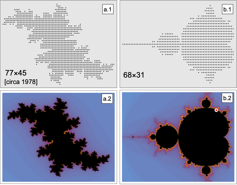
Figure 1: Julia and MBM sets. The top row shows the Julia set (a.1) for $f(z)=z^{2}+C$ with $C=0.1+0.6\,i$ and the Mandelbrot-Brooks-Matelski (MBM) set (b.1) reproduced from the original work of Brooks and Matelski Brooks and Matelski (1981). The bottom row presents high-resolution, colorized versions of these sets, generated using Wolfram Mathematica built-in functions. The red point in (b.2) corresponds to $0.1+0.6\,i$.

All three sets arise from iterating the quadratic map:

$$z\mapsto z^{\prime}=z^{2}+C,\qquad\qquad z\in\mathbb{C},$$

with complex parameter

$$C\in\mathbb{C},$$

but each set, however, explores a distinct aspect of the system. The MBM set identifies all complex values of $C$, for which the iteration, starting from $z_{0}=0$ remains bounded. Within the Mandelbrot set, the behavior of the system is stable. These stable regions correspond to black areas in visualizations, while points outside the set represent parameters where the orbit diverges. These diverging regions are often color-coded to reflect the rate of escape, see plot (b.2) in Fig. 1. The boundary of the Mandelbrot set is a fractal, infinitely complex and self-similar, serving as a control plot for mapping stability.

Each point in the Mandelbrot set corresponds to a unique Julia set, linking parameter space to phase space, for instance, the red point in plot (b.2) corresponds to the Julia set depicted in plot (a.2). Julia sets examine the dynamics for a fixed parameter $C$, focusing on the phase space of initial conditions $z_{0}$. These sets form the boundary between points that generate bounded orbits and those that escape to infinity. When $C$ lies inside the Mandelbrot set, the corresponding Julia set is connected, resembling a cohesive fractal structure. Conversely, if $C$ is outside the Mandelbrot set, the Julia set is a Cantor set, consisting of disconnected points scattered across the plane. The boundary of the Julia set is where chaotic dynamics dominate, with points neither escaping nor converging but instead forming fractal patterns. Fatou set complements this picture, representing regions of phase space where the dynamics are smooth and predictable, such as convergence to fixed points or periodic orbits.

Real plane mappings provide two other prominent examples of quadratic iterations: the dissipative Hénon–Pomeau map Hénon (1976), characterized by its strange attractor and two parameters, and the area-preserving quadratic Hénon map Hénon (1969), which depends on a single parameter. Both are among the most extensively studied dynamical systems of the plane.

We speculate that the Hénon–Pomeau attractor has garnered greater attention due to its broader range of applications. Notably, in 1993, a colored version of the control plot illustrating the structure of its parameter space was published in Gallas (1993). In contrast, the area-preserving Hénon map has received significant theoretical attention Sterling et al. (1999); Dullin and Meiss (2000); Dullin et al. (2000), with its phase space diagrams setting the standard for illustrating chaotic dynamics. Yet, despite its theoretical prominence, comprehensive visualizations of its mixed variable-parameter space remain limited, even though this was originally attempted in Hénon’s seminal work.

This set was intended to be a control plot, summarizing the continuum of two-dimensional phase space portraits into a two-dimensional representation of the mapping’s parameter and a coordinate along the symmetry line, Fig. 2. However, much like the original image generated by Brooks and Matelski, which was limited to under 100 pixels in each dimension (approximately 1 kilopixel), the resolution of the Hénon set — restricted to $199\times 159$ pixels (about 30,000 sample trajectories) — lacked the clarity needed to capture the full intricacy of the system’s dynamics.

Modern computational tools, such as the built-in functions MandelbrotSetPlot[] and JuliaSetPlot[] introduced in Wolfram Mathematica 10.0 Inc. (2013), provide efficient visualization of the MBM set, enabling the creation of high-resolution, detailed images in seconds (bottom row in Fig. 1). However, similar advances in visualizing the combined parameter-variable spaces of the area-preserving Hénon map have not been fully realized. As a result, the intricate dynamics of this mapping remain partially obscured, underscoring the need for further exploration and development of visualization techniques tailored to such systems.

More importantly, beyond its low resolution, there is a fundamental qualitative issue: the dramatic reduction of a 2D phase space to a 1D representation of initial conditions led to the loss of crucial information, a limitation that Hénon himself observed. This gap in understanding highlights the need for a renewed exploration of these structures, inspired by the numerous classical studies.

This article aims to address several interconnected goals:

(i) Our investigation began with an effort to identify missing features in Hénon’s diagram, which led us to explore the concepts of reversibility, associated symmetries, and their implications for invariant sets. These ideas, though not completely recognized by Hénon at the time, had been anticipated by G.D. Birkhoff during the same period as Fatou and Julia’s pioneering research (please see Lewis Jr. (1961) for the list of references). In the 1950s, René J. DeVogelaere DeVogelaere (1958) further developed this understanding, and later, E. McMillan utilized these symmetries to discover his integrable systems McMillan (1971). Despite these advances, as noted in J.A.G. Roberts’ and G.R.W. Quispel’s comprehensive review Roberts and Quispel (1992), awareness of these concepts has remained limited across different scientific disciplines. In Subsections III.2 and III.3, we revisit and consolidate key properties of these symmetries. Further, in Subsections III.4 and III.5, we discuss how these symmetries extend beyond isolated periodic orbits to groups of such orbits that emerge in typical bifurcations. In doing so, we propose extending the original isochronous diagram introduced by Hénon, which captures bifurcations of fixed points, to include additional period-doubling diagram for 2-cycles and, where applicable, further diagrams for cases of multiple reversibility. This collection of two-dimensional plots significantly reduces the complexity of analyzing the original three-dimensional space of two variables and a parameter, while effectively revealing the locations of previously overlooked symmetric periodic orbits.

(ii) In Section IV, we examine modern visualization techniques to study dynamical regimes Bazzani et al. (2023); Das et al. (2017). These include mode-locking, Frequency Map Analysis (FMA) Laskar (1999, 2003), the Reversibility Error Method (REM) Panichi et al. (2016, 2017), and the Generalized Alignment Index (GALI) Skokos et al. (2007); Skokos and Manos (2016). We demonstrate that REM and GALI are not only effective tools for distinguishing between regular and chaotic dynamics in phase space but also highly efficient at detecting bifurcations of isolated periodic trajectories in parameter space. Furthermore, these methods can pinpoint twistless bifurcations, which are associated with the emergence of non-isolated structures in phase space.

(iii) Section V provides a qualitative description of stability diagrams using models such as the chaotic Arnold circle map and the integrable McMillan mappings. For a more comprehensive treatment, an auxiliary article Zolkin et al. (2024a) examines the intricate relationships between McMillan integrable systems and typical chaotic mappings in standard form. Using the twist variable, which measures the derivative of the rotation number with respect to the action variable, we offer a quantitative description of small-amplitude dynamics and investigate some numerical aspects of resonance overlap at larger amplitudes. A dedicated Subsection V.4 explores the twistless orbit and the bifurcations it induces, including its impact on Arnold tongues.

(iv) Finally, in Section VI, we provide diagrams for various homogeneous power function Hénon mappings that are directly linked to horizontal dynamics in model accelerator lattices, incorporating thin nonlinear magnets such as sextupoles, octupoles, decapoles, and duodecapoles. Additionally, we analyze the Chirikov Chirikov (1971, 1979) mapping, which models longitudinal motion in accelerator rings with thin RF stations. This section bridges theoretical concepts with practical applications, underscoring the relevance of our findings.

II Hénon set

In Hénon’s original article Hénon (1969), he considered an area-preserving (symplectic) mapping of the plane ($\mathbb{R}^{2}\mapsto\mathbb{R}^{2}$) defined as follows:

$$\mathrm{T}_{2}:\qquad\begin{array}[]{l}x^{\prime}=g_{2}(x,y),\\[7.11317pt] y^{\prime}=h_{2}(x,y),\end{array}$$

where the $(^{\prime})$ symbol denotes the application of the map, and $g_{2}$ and $h_{2}$ are second-degree polynomials:

$$\begin{array}[]{r}g_{2}(x,y)=a_{1}\,x+b_{1}\,y+c_{1}\,x^{2}+d_{1}\,x\,y+e_{1}\,y^{2},\\[7.11317pt] h_{2}(x,y)=a_{2}\,x+b_{2}\,y+c_{2}\,x^{2}+d_{2}\,x\,y+e_{2}\,y^{2}.\end{array}$$

Assuming a stable invariant point at the origin:

$$\big{|}\operatorname{tr}\,\mathrm{d}\mathrm{T}_{2}(x,y=0)\big{|}<2$$

and using the fact that for an area-preserving map, the Jacobian determinant must be equal to one:

$$\boldsymbol{\mathrm{J}}=\det\mathrm{d}\mathrm{T}_{2}=\begin{vmatrix}\partial x^{\prime}/\partial x&\partial x^{\prime}/\partial y\\[7.11317pt] \partial y^{\prime}/\partial x&\partial y^{\prime}/\partial y\end{vmatrix}=1,$$

Hénon was able to show that by a linear change of coordinates, the transformation can be reduced to a much simpler form:

$$\mathrm{T}:\qquad\begin{array}[]{r}\displaystyle x^{\prime}=x\,\cos\psi-\left[y-F(x)\right]\,\sin\psi,\\[7.11317pt] \displaystyle y^{\prime}=x\,\sin\psi\,+\left[y-F(x)\right]\cos\psi,\end{array}$$ (1)

with only one intrinsic parameter $\psi$ remaining, and quadratic force function $F(x)=x^{2}$. This parameter is irreducible and represents the rotation angle in the infinitesimal vicinity of the origin, providing a rotation number of the fixed point:

$$\nu_{0}=\frac{\psi}{2\,\pi},$$

which is independent of the mapping’s representation.

He discussed some properties of the mapping, including certain invariant points: fixed points ($n=1$) and low order $n$-cycles ($n=2,3,4$), defined as

$$(x,y)=\mathrm{T}^{n}(x,y),\qquad\qquad n\in\mathbb{Z}.$$

For the readers’ convenience, we provide all analytical expressions relevant to the discussion of periodic orbits and their domains of stability in Appendix A at the end of this article. Next, he acknowledged that mapping (1) and its inverse can be seen as a convolution of two simpler area-preserving transformations:

$$\mathrm{T}=\mathrm{Rot}(\psi)\circ\mathrm{S}_{-F},\qquad\qquad\mathrm{T}^{-1}=\mathrm{S}_{F}\circ\mathrm{Rot}(-\psi),$$

where $\mathrm{Rot}(\psi)$ is the rotation about the origin by an angle $\psi$:

$$\mathrm{Rot}(\psi)=\mathrm{Rot}^{-1}(-\psi):\quad\begin{bmatrix}x^{\prime}\\[7.11317pt] y^{\prime}\end{bmatrix}=\begin{bmatrix}\cos\psi&-\sin\psi\\[7.11317pt] \sin\psi&\cos\psi\end{bmatrix}\begin{bmatrix}x\\[7.11317pt] y\end{bmatrix},$$

and $\mathrm{S}_{\pm F}$ is a nonlinear vertical shear:

$$\mathrm{S}_{\pm F}=\mathrm{S}^{-1}_{\mp F}:\qquad\begin{array}[]{ll}x^{\prime}=x,\\[7.11317pt] y^{\prime}=y\pm F(x).\end{array}$$

He further remarked on the existence of the symmetry line

$$L_{1}:\qquad y=x\,\tan[\psi/2]$$

which explains the bilateral (mirror) symmetry in phase-space portraits (refer to the dashed green line in Fig. 2) and is associated with the form of the map, but not the specific form of the force function $F(x)$. For illustrations we reconstructed and slightly updated to match our notation his original plots and combined them in Fig. 2; as some of his plots were hand drawn, and, in order to incorporate some additional information minor stylistic changes were made, while attempting to preserve its original spirit.

He then analyzed long-term stability through numerical experiments/tracking, utilizing several hundred iterates for each orbit in specific case studies across various values of the mapping parameter $\psi$ (plots [H1]–[H10] in Fig. 2). Moreover, he attempted to capture the entirety of dynamical regimes in a 2D symbol plot (the main plot [H0] at the top left), where orbit types were described as a function of the initial position along the symmetry line $L_{1}$ and the value of $\nu_{0}$. He distinguished three types of trajectories: those that orbit the origin on a closed curve (stable), those that follow closed curves around chains of islands (mode-locked), and those that disperse to infinity (unstable). However, as mentioned in Hénon (1969), certain important details, such as even chains of islands, were sometimes missed, indicating an incompleteness in the summarized depiction compared to the full 2D phase-space dynamics:

…Plot [H3] exhibits a string of 5 large islands. One of the islands is situated on the positive $L_{1}$ axis; this explains the large band on plot [H0]. The same plot [H0] shows that these islands move away from the center and grow larger when $\nu_{0}$ increases; they are first inside the curve region (this is the case for plot [H3]), then outside. Similar bands appear on plot [H0] for smaller values of $\nu_{0}$; they correspond to strings of 7 and 9 islands. The chain of 6 islands of plot [H2] does not appear on plot [H0] because none of the islands is on the axis of symmetry. (Incidentally, it seems that all strings with an even number of islands possess this property, namely, the centers of the islands are never on the axis of symmetry. We have not been able to find an explanation for this observed fact.)…

In the following, we explore the mystery surrounding Hénon’s set — a question partially addressed by G.D. Birkhoff — and examine additional methods to enrich the original fractal structure, making it even more informative.

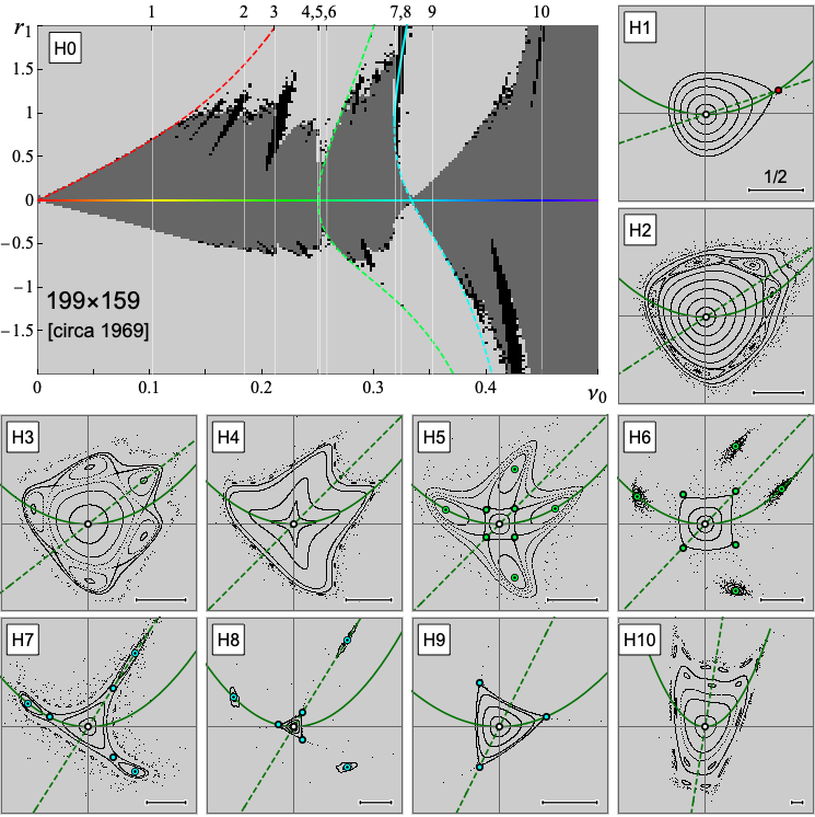
Figure 2: Hénon set. The main plot at the top [H0] serves as a summary for all values of $\nu_{0}$, depicting distance $r_{1}$ to initial points along the first symmetry line $L_{1}$ (after Hénon Hénon (1969)). Pixels in different colors correspond to various trajectory types: light gray indicates escape, dark gray represents successive points on a closed curve, and black denotes points on a string of islands. Full and dashed curves depict stable and unstable $n$-cycles for $n=1,\ldots,4$ respectively, with color indicating the rotation number calibrated by $\nu_{0}$. Vertical marks and letters above refer to corresponding phase-space portraits $(x,y)$, [H1]–[H10], each displaying several sample trajectories (black dots), isolated $n$-cycles (same color as in the summary plot), and both symmetry lines (dashed and solid curves in dark green for $L_{1}$ and $L_{2}$ respectively).

III Missing islands

III.1 Form of the map

Before addressing the issue of missing islands, we may benefit from making a few key adjustments. While the form of map (1) is already quite straightforward, we introduce an alternative representation referred to here as the McMillan form (see, e.g., McMillan (1971); Turaev (2002); Zolkin et al. (2023, 2024b) for details):

$$\mathrm{M}:\qquad\begin{array}[]{l}q^{\prime}=p,\\[7.11317pt] p^{\prime}=-q+f(p).\end{array}$$ (2)

The two forms of the map are related by a change of variables:

$$\begin{array}[]{ll}x=p,&\qquad q=x\,\cos\psi+y\,\sin\psi,\\[7.11317pt] y=q\,\csc\psi-p\,\cot\psi,&\qquad p=x,\end{array}$$ (3)

with a modified force function:

$$f(x)=2\,x\,\cos\psi+F(x)\,\sin\psi.$$

While the determinants of these transformations (3) are constant and independent of dynamical variables, they differ from unity, introducing additional scaling:

$$-\csc\psi\qquad\text{and}\qquad-\sin\psi.$$ (4)

(i) Hénon’s consideration of general second-degree polynomials was constrained by the requirement for a stable fixed point at the origin, ruling out dynamics beyond the period-doubling bifurcation. This could be addressed by using a hyperbolic rotation instead of the standard rotation matrix, though this requires a further modification of the map’s linear “normal” form. Parametrizing the new force function as

$$f(q)=a\,q+q^{2},$$

the McMillan form allows a trace with an absolute value greater than 2, extending the range of possible dynamical regimes.

(ii) The Hénon set extends along $L_{1}$ when $\nu_{0}$ approaches a half-integer (1/2), growing infinitely. The scaling from Eq. (4) allows us to adjust the fractal size, making it easier to examine large-amplitude details in this parameter range. Subsection V.2 discusses the implications of this scaling in greater detail.

(iii) The McMillan form of the map can also be decomposed as a composition of two simpler symplectic mappings:

$$\mathrm{M}=\mathrm{S}_{f}\circ\mathrm{Rot}(\pi/2),\qquad\mathrm{M}^{-1}=\mathrm{Rot}(-\pi/2)\circ\mathrm{S}_{-f}.$$

Additionally, as noted by E. McMillan McMillan (1971), there is another decomposition:

$$\mathrm{M}=\mathrm{R}_{f}\circ\mathrm{Ref}(\pi/4),\qquad\quad\,\mathrm{M}^{-1}=\mathrm{Ref}(\pi/4)\circ\mathrm{R}_{f},$$

where $\mathrm{Ref(\psi)}$ represents a reflection about a line through the origin at angle $\psi$ with the $q$ axis:

$$\mathrm{Ref}(\psi):\quad\begin{bmatrix}q^{\prime}\\[7.11317pt] p^{\prime}\end{bmatrix}=\begin{bmatrix}\cos 2\psi&\sin 2\psi\\[7.11317pt] \sin 2\psi&-\cos 2\psi\end{bmatrix}\begin{bmatrix}q\\[7.11317pt] p\end{bmatrix}$$

and $\mathrm{R}_{f}$ is a nonlinear vertical reflection:

$$\mathrm{R}_{f}:\qquad\begin{array}[]{ll}q^{\prime}=q,\\[7.11317pt] p^{\prime}=-p+f(q).\end{array}$$

Both reflections ($\mathrm{R}$) have a Jacobian determinant of $-1$, making them involutory transformations with

$$\mathrm{R}^{-1}=\mathrm{R},\qquad\mathrm{R}^{2}=\mathrm{I}_{2},$$ (5)

where $\mathrm{I}_{2}$ is the $2\times 2$ identity matrix. As a result, each reflection has a line of fixed points:

$$l_{1}:\,\mathrm{Fix}\,[\mathrm{Ref}(\pi/4)]=\left\{(q,p)|\,p=q\right\}$$

and

$$l_{2}:\,\mathrm{Fix}\,[\mathrm{R}_{f}]=\left\{(q,p)|\,p=f(q)/2\right\},$$

with all other initial conditions forming 2-cycles under $\mathrm{R}_{1,2}$, according to Eq. (5). Thus, this decomposition reveals two symmetry lines.

For the transformation in its original form, we have:

$$\mathrm{T}=\mathrm{Ref}(\psi/2)\circ\mathrm{R}_{F},\qquad\quad\,\mathrm{T}^{-1}=\mathrm{R}_{F}\circ\mathrm{Ref}(\psi/2),$$

with corresponding first and second symmetry lines:

$$L_{1}:\,y=x\,\tan(\psi/2)\qquad\text{and}\qquad L_{2}:\,y=F(x)/2.$$

Comparing these two forms of the map, we see that in the McMillan form, the first symmetry line $l_{1}$ is fixed and independent of $f(q)$, while in Hénon’s form, the first symmetry line $L_{1}$ rotates as $\nu_{0}$ increases, and the second symmetry $L_{2}$ is determined solely by $F(q)$, which is independent of $\psi$.

Another modification we adopt in the McMillan form, unlike Hénon’s original setup, is to use the horizontal projection onto the $q$-axis, denoted $q_{1,2}$ for $L_{1,2}$, instead of measuring distance along the symmetry line $q_{1}^{\dagger}$. This projection is simpler than calculating distance, especially for the second symmetry, which is defined by a curve rather than a line. In the Hénon form, however, using this projection is less convenient, as the orientation of $L_{1}$ depends on $\psi$.

Long before McMillan’s work, G.D. Birkhoff and, later, R. deVogelaere DeVogelaere (1958) had already explored the decomposition of transformations into two involutions, highlighting the significance of reversibility in a series of publications from 1914 to 1945 (see Lewis Jr. (1961) and references therein). In the following section, we review the fundamental properties of reversibility and consider its implications, laying the groundwork for a deeper understanding.

III.2 Symmetry lines and reversibility

Despite the long history of time-reversibility, A.J. Roberts observed in his 1992 report Roberts and Quispel (1992) that “…reversible dynamical systems have received far less attention and the treatment that they have received has tended to be less systematic. This has led to the situation where the literature on the subject is quite scattered, with some authors not being aware of the generality of the mathematical theory underlying their results.” Here, we summarize relevant findings from Lewis Jr. (1961); DeVogelaere (1958), as well as Roberts and Quispel (1992), to provide context for further discussion.

A transformation $\mathrm{T}$ is termed reversible, if it can be expressed as a composition of two involutions:

$$\mathrm{T}=\mathrm{R}_{2}\circ\mathrm{R}_{1},\qquad\qquad\mathrm{R}_{1,2}^{2}=\mathrm{I}_{2},$$ (6)

where $\mathrm{R}_{1}$ and $\mathrm{R}_{2}$ are the reversing symmetries of $\mathrm{T}$. As discussed in detail in Roberts and Quispel (1992), this definition of reversibility does not require $\mathrm{T}$ to be conservative, area-preserving, measure-preserving, or even to operate on an even-dimensional manifold. For a reversible map (6), we find:

$$\mathrm{R}_{1}=\mathrm{R}_{2}\circ\mathrm{T}=\mathrm{T}^{-1}\circ\mathrm{R}_{2},\quad\,\,\mathrm{R}_{2}=\mathrm{T}\circ\mathrm{R}_{1}=\mathrm{R}_{1}\circ\mathrm{T}^{-1},$$

which ensures that $\mathrm{T}$ is invertible, with

$$\mathrm{T}^{-1}=\mathrm{R}_{1}\circ\mathrm{R}_{2}.$$

This implies that the map and its inverse are conjugate to each other, as there exists an invertible conjugating transformation $\mathrm{P}$ such that

$$\mathrm{T}^{-1}=\mathrm{P}\circ\mathrm{T}\circ\mathrm{P}^{-1},$$ (7)

because, for both symmetries, we have

$$\mathrm{T}^{-1}=\mathrm{R}_{1}\circ\mathrm{T}\circ\mathrm{R}_{1}\quad\text{and}\quad\mathrm{T}^{-1}=\mathrm{R}_{2}\circ\mathrm{T}\circ\mathrm{R}_{2}.$$

Mappings that satisfy (7) with $\mathrm{P}$ not necessarily an involution are considered weakly reversible.

As deVogelaere noted DeVogelaere (1958), if $\mathrm{R}$ is a reversing symmetry of $\mathrm{T}$, then so is the entire family of symmetries $\left\{\mathrm{T}^{k}\circ\mathrm{R}\right\}$, forming an infinite group along with the iterates of the map $\left\{\mathrm{T}^{k}\right\}$. A map can also possess additional, independent families of reversing symmetries, not necessarily but often weakly reversible, in which case it is called a multiply reversible map. A notable case discussed in Roberts and Quispel (1992) is that of doubly reversible mappings, such as reversible odd maps, where $\mathrm{T}$ commutes with the rotation $\mathrm{Rot}(\pi)$.

Lastly, the set of fixed points of $\mathrm{R}$, $\mathrm{Fix}\,\mathrm{R}$, and those of $\mathrm{Fix}\,\mathrm{T}^{n}\mathrm{R}$, form an infinite family of symmetry lines. When $\mathrm{R}$ is an orientation-reversing $C^{1}$ involution of the plane, these lines are non-intersecting and do not terminate, remaining analytic if $\mathrm{R}$ is analytic, as originally discussed in J.D. Finn’s dissertation. For maps in Hénon form, we denote the symmetry lines as $L_{1,2}$, while in McMillan form, we use $l_{1,2}$ for the first two symmetry lines $\mathrm{Fix},\mathrm{R}_{1,2}$.

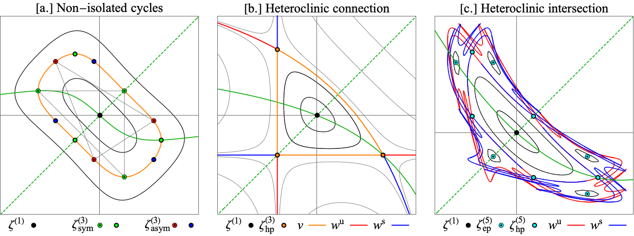
Figure 3: Invariant orbits. Plot (a.) demonstrates non-isolated $n$-cycles using the McMillan map with $f(q)=-\frac{9}{5}\,q/(q^{2}+1)$. The closed orange curve represents an invariant level set with rotation number $1/3$. Symmetric orbits are shown in green, while asymmetric orbits appear in blue and red. Connecting lines illustrate iterations between points. Plot (b.) shows a heteroclinic connection in another integrable McMillan map, $f(q)=\frac{16}{5}\,q/(q-4)$. Red and blue curves depict the unstable ($w^{\mathrm{u}}$) and stable ($w^{\mathrm{s}}$) manifolds associated with the hyperbolic 3-cycle $\zeta^{(3)}_{\mathrm{hp}}$, with the heteroclinic connection $v$ in orange. Plot (c.) uses the chaotic Hénon map $f(q)=-\frac{9}{5}\,q+q^{2}$, revealing a chain of 5 islands with stable and unstable manifolds intersecting heteroclinically. In all plots, the fixed point at the origin is marked in black, while other periodic orbits are colored as per legend. Black orbits represent irrational rotations, and gray in (b.) indicates unstable trajectories. Green dashed and solid lines denote the first, $p=q$, and second, $p=f(q)/2$, symmetry lines.

III.3 Invariant sets

In this subsection, we define and review some fundamental properties of invariant sets and orbits in area-preserving mappings, following Roberts and Quispel (1992). Fig. 3 illustrates these concepts with phase space portraits of various integrable and chaotic systems.

For a stable orbit of a point $\zeta_{0}=(q_{0},p_{0})$ under an area-preserving mapping $\mathrm{T}$, the trajectory typically exhibits one of three behaviors in phase space:

(i) The trajectory forms a zero-dimensional set of $n$ distinct points visited in a unique periodic sequence:

$$\mathrm{T}^{n}\zeta_{0}=\zeta_{0},\qquad\qquad n>0.$$ (8)

This set of points is called an $n$-cycle:

$$\zeta^{(n)}=\left\{\zeta_{0},\zeta_{1},\ldots,\zeta_{n-1}\right\},$$

or a fixed point if $n=1$. In Fig. 3 the fixed point at the origin is shown in black, while other periodic orbits ($n>1$) are color-coded.

(ii) The trajectory forms a one-dimensional set that lies on an invariant curve, $C$, in the plane. In chaotic systems, these curves correspond to KAM curves or circles and are densely filled in a quasiperiodic manner. The rotation number for such curves is irrational, resulting in an angular increment that is incommensurate with $2\,\pi$ (black closed curves in all plots). In nonlinear integrable systems, however, the rotation number is often a continuous function of amplitude. Consequently, when $\nu$ crosses rational values $m/n$, such invariant curves break into an infinite number of $n$-cycles, as shown by the orange curve in plot (a.). We refer to these as non-isolated $n$-cycles, in contrast to isolated $n$-cycles, which lack other orbits of the same period nearby (provided their eigenvalues are not roots of unity). In chaotic systems, rational rotation numbers typically correspond to centers $\zeta^{(n)}_{\mathrm{ep}}$ (elliptic periodic points) or nodes $\zeta^{(n)}_{\mathrm{hp}}$ (hyperbolic periodic points) of island chains.

(iii) The trajectory appears to wander without period or quasiperiodicity, densely covering a region of the phase space. In these cases, the orbit exhibits exponential sensitivity to initial conditions and is classified as chaotic.

A set of points, $\Gamma$, is called invariant under the mapping $\mathrm{T}$, if $\mathrm{T}\,\Gamma=\Gamma$. Thus, by definition (8), all points in an $n$-cycle form an invariant set. Likewise, a curve $C$ on the plane can be invariant if

$$\forall\,\zeta\in C:\qquad\zeta^{\prime}=\mathrm{T}\,\zeta\in C.$$

In Fig. 3, all closed curves around the fixed point at the origin are invariant, while a curve surrounding one of the five islands (in plot c.) is not; here, each curve is sequentially visited, making all five curves together an invariant set.

Stable (elliptic) periodic points are typically surrounded by elliptical orbits, hence the name. In contrast, each point in an unstable (hyperbolic) $n$-cycle has associated stable ($w^{\mathrm{s}}$) and unstable ($w^{\mathrm{u}}$) manifolds:

$$w^{\mathrm{s,u}}\left[\zeta^{(n)}_{k}\right]=\left\{\zeta_{0}\,:\,\lim_{N\rightarrow\infty}\mathrm{T}^{\pm(n\cdot N)}\zeta_{0}=\zeta^{(n)}_{k}\right\}$$

aligned with the eigenvectors of $\mathrm{d}\mathrm{T}^{n}[\zeta^{(n)}_{k}]$ near $\zeta^{(n)}_{k}$. For $n>1$, the orbit hops between branches of the same stability (similar to transitioning between islands) while following the manifolds either toward or away from the cycle. Thus, all stable or all unstable branches collectively form another example of an invariant set.

In integrable systems, these manifolds may extend to infinity (as shown by the red and blue curves in plot b.) or form a connection (orange curve):

$$v=w^{\mathrm{s}}\left[\zeta^{(n)}_{i}\right]\bigcap w^{\mathrm{u}}\left[\zeta^{(n)}_{j}\right]$$

called heteroclinic if $i\neq j$ or homoclinic if the point connects to itself, $i=j$. In chaotic systems, stable and unstable manifolds may intersect, forming an intricate, ongoing network of heteroclinic/homoclinic intersections — often called tangles (see plot c.).

We note that if $\Gamma$ is an invariant set, then so is $\mathrm{R}\,\Gamma$, where $\mathrm{R}$ is one of the involutions of $\mathrm{T}$. For example, the stable (unstable) manifold of a point $\zeta^{(n)}_{k}$ maps under $\mathrm{R}$ to the unstable (stable) manifold of $\mathrm{R}\,\zeta^{(n)}_{k}$. An invariant set is termed symmetric, if it is invariant under both $\mathrm{T}$ and $\mathrm{R}$. This definition can apply to a curve, a periodic or aperiodic orbit, or a collection of such objects.

As McMillan observed McMillan (1971), for integrable systems, constant level sets, $\mathcal{K}[p,q]=\mathrm{const}$, must be symmetric:

$$\mathcal{K}[\zeta_{0}]=\mathcal{K}[\mathrm{T}\,\zeta_{0}]\quad\text{and}\quad\mathcal{K}[\zeta_{0}]=\mathcal{K}[\mathrm{R}\,\zeta_{0}].$$

In chaotic systems, these level sets correspond to collections of orbits sharing an “energy” level that persists despite perturbations. In plot (a.) of Fig. 3, the closed orange curve with a rotation number of $1/3$ represents a symmetric invariant set. Among the trajectories on it, only the two shown in green are symmetric by themselves. Other orbits, such as those shown in red and blue, are asymmetric. However, the red and blue orbits are constructed as reflections of each other with respect to $\mathrm{R}$ and, as a pair, they form a symmetric invariant set (not an orbit!).

The same principle applies to manifolds $w^{\mathrm{u,s}}$, which, while individually invariant only under $\mathrm{T}$, together form a symmetric set. However, in this case, the intersection of the two unions, $\mathrm{V}=\Gamma\bigcap\mathrm{R}\,\Gamma$, can be nonempty, making $\mathrm{V}$ a symmetric invariant (strict) subset of $\Gamma$. Thus, invariant sets generally consist of symmetric invariant subsets alongside pairs of asymmetric subsets. For instance, in plot (b.) we observe a symmetric 3-cycle along with a pair of associated stable and unstable manifolds. In contrast, plot (c.) presents a scenario where, instead of a periodic symmetric subset, we have a symmetric orbit that intersects both manifolds and exhibits perpetual wandering.

III.4 Symmetric groups

Since for any point in a symmetric orbit, $\zeta\in\Gamma_{\mathrm{sym}}$,

$$\exists\,k\in\mathbb{Z}:\,\,\mathrm{R}\,\zeta=\mathrm{T}^{k}\zeta\in\Gamma_{\mathrm{sym}},$$

its trajectory must “hop across” the symmetry line if $k$ is odd,

$$\mathrm{T}^{-1}\circ\mathrm{R}\,\left(\mathrm{T}^{(k-1)/2}\zeta\right)=\mathrm{T}^{(k-1)/2}\zeta$$ (9)

or “cross” it if $k$ is even,

$$\mathrm{R}\,\left(\mathrm{T}^{k/2}\zeta\right)=\mathrm{T}^{k/2}\zeta.$$ (10)

Conversely, if a trajectory crosses (10) the symmetry line $\mathrm{Fix}\,\mathrm{R}$, it is symmetric with respect to $\mathrm{R}$ and the entire family of symmetries $(\mathrm{T}^{n}\circ\mathrm{R})$. This is evident as each point of its orbit lies on the symmetry line according to

$$\begin{array}[]{l}\mathrm{T}^{i}\,\mathrm{Fix}\,(\mathrm{R}_{1})=\mathrm{Fix}\,(\mathrm{T}^{2\,i}\circ\mathrm{R}_{1}),\\[7.11317pt] \mathrm{T}^{i}\,\mathrm{Fix}\,(\mathrm{R}_{2})=\mathrm{Fix}\,(\mathrm{T}^{2\,i+1}\circ\mathrm{R}_{1}).\end{array}$$ (11)

If a point lies at the intersection of two distinct symmetry lines, it is termed doubly symmetric. Each doubly symmetric point is periodic under $\mathrm{T}$, and each symmetric periodic point is doubly symmetric Lewis Jr. (1961); DeVogelaere (1958), as indicated by

$$(\mathrm{T}^{m}\circ\mathrm{R})\circ(\mathrm{T}^{n}\circ\mathrm{R})\,\zeta=\mathrm{T}^{m-n}\,\zeta=\zeta.$$ (12)

Thus, for symmetric periodic orbits, each point lies on an intersection of the entire subfamily of symmetries. Eqs. (11,12) further imply that if $\zeta$ and $\mathrm{T}^{r}\zeta\neq\zeta$ lie on the same symmetry line, the orbit has an even period of $2r$. Moreover, a symmetric periodic orbit has an even period if and only if it includes two points on the same symmetry line.

While much attention has been given to symmetric periodic orbits, isolated cycles with similar stability can appear in degenerate groups — on the same energy level — alongside asymmetric orbits. As we’ll see, such groups often split. To clarify the dynamics of these groups, we consider a symbolic model illustrated in Fig. 4. In this model, a symmetric group of $n$ points (in black) is divided evenly by each of the two symmetry lines (in green). Each iteration, $\mathrm{T}=\mathrm{R}_{2}\circ\mathrm{R}_{1}$, is a sequential application of two involutions, here represented by linear reflections $\mathrm{Ref}(\theta)$. By aligning the first symmetry line with the horizontal axis ($\theta_{1}=0$), and using

$$\mathrm{Ref}(\theta_{2})\circ\mathrm{Ref}(\theta_{1})=\mathrm{Rot}(2\,\theta_{2}-2\,\theta_{1})$$

we see that the rotation number must satisfy

$$\nu=2\,k/n$$

where $k$ is the angle between symmetries divided over $2\,\pi$.

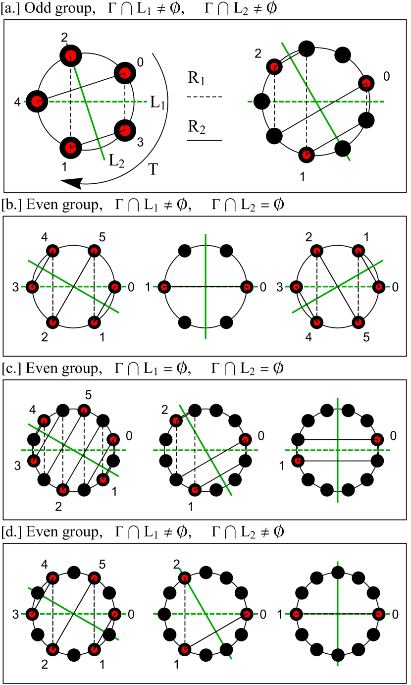
Figure 4: Symmetric groups. Plot (a.) illustrates the dynamics of odd symmetric groups with $n=5$ and $9$ points. The next three plots show the dynamics of even symmetric groups: one that intersects only a single symmetry line (b.), one that intersects no symmetry lines (c.), and one that intersects both (d.). In all plots, the first symmetry line $L_{1}=\mathrm{Fix}\,\mathrm{R}_{1}$ is shown as a dashed green horizontal line, and the second symmetry line $L_{2}=\mathrm{Fix}\,\mathrm{R}_{2}$ is solid. Dashed and solid black lines represent the iterates of a point under the reflections $\mathrm{R}_{1,2}$, respectively. Each diagram includes a sample periodic orbit (in red), with numerals indicating the iterate number. Since the combination of two reflections is equivalent to a rotation, the orbits traverse the intersection of the symmetry lines in a clockwise direction.

For an odd symmetric group or individual $n$-cycle, geometry dictates that each symmetry line contains one point of the group/cycle, as this is the only way to evenly split an odd group. These orbits cannot have more than one crossing per line, implying an even period. If $\nu$ is a reducible fraction, the group splits into $n/m$ $m$-cycles, where $l/m$ is an irreducible form of $\nu$, as illustrated in Fig. 4 (a.) for $n=9$ and $2\,k=3$.

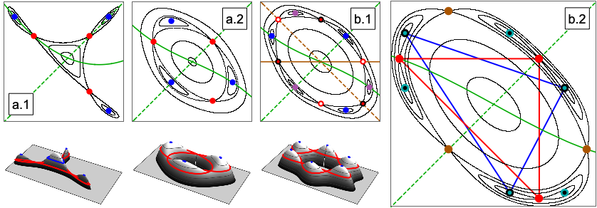
Figure 5: Islands and symmetries. The top row shows phase-space portraits for various Hénon mappings with force functions of the form $f(q)=a\,q+b\,q^{2}+c\,q^{3}$. Each plot illustrates the result of a specific bifurcation, with the corresponding triplets of coefficients $[a,b,c]$: (a.1) saddle-node ($\mathrm{SN}_{1/3}$) $[-0.84,1,0]$, or a touch-and-go bifurcation if the image is cropped to remove the blue points; (a.2) 3-island chain $[-0.9,0.02,-1]$; (b.1) doubled 3-island chain $[-0.85,0,-1]$; and (b.2) asymmetric split $[-1.1,6\times 10^{-3},1]$. The bottom row illustrates the invariant level sets of an integrable system with a similar phase-space topology. In all plots, isolated 3-cycles are shown in color, and the first and second symmetry lines are indicated by solid and dashed green lines. Plot (b.1) also shows an additional independent family of symmetries in brown.

For odd symmetric cycles or groups, there is a single crossing and one hop per symmetry line. In contrast, even groups are more complex: each symmetry line may exhibit either two crossings or two hops. Symmetric even cycles can only cross one symmetry line or must split, as shown in Fig. 4 (d.). Degeneracies occur again if $\nu$ is reducible, as illustrated in the middle diagram of Fig. 4 (b.) for $n=6$ and $2\,k=3$.

The two bottom plots explore cases where the even group crosses neither symmetry line (c.) or both symmetry lines (d.). In these cases, both $2\,k$ and $n$ must be even, requiring the group to split, at least in half, consistent with the fact that symmetric even cycles cannot cross both lines. Only in case (c.) does the group completely disappear. In all other cases, even with degeneracies, at least one symmetry line intersects one of the orbits. Asymmetric periodic orbits that do not cross symmetry lines appear in pairs. Thus, although these orbits do not lie on symmetry lines (case c.), if they represent centers or nodes of chains of islands, the connections and intersections of their surrounding manifolds $w^{\mathrm{u,s}}$ must form symmetric sets.

III.5 Islands and bifurcations

Finally, we apply the insights we’ve gathered to understand how island chains, which emerge from typical bifurcations around fixed points, interact with the two primary symmetry lines. While we do not aim to fully classify symplectic map bifurcations, we follow Barrio and Blesa (2009) and refer the reader to Abraham and Marsden (1978) for a comprehensive description.

All fixed points and 2-cycles lie on intersections at $L_{1}\cap L_{2}$ and $L_{2}\cap L_{2}^{-1}$, respectively. Thus, by analyzing both symmetry lines, we reliably encounter isochronous bifurcations (i.e., those involving appearance or disappearance of solutions without changing cycle frequency), such as transcritical (T), saddle-node (SN), pitchforks (PF), and period-doubling (PD) bifurcations. Accordingly, we suggest naming diagrams along $L_{1}$ as isochronous and those along $L_{2}$ as period-doubling diagrams.

Turning to cycles with periods $n\geq 3$, Figure 5 illustrates examples of more complex bifurcations through phase-space plots, featuring isolated period-3 orbits.

Touch-and-Go (TG): In this simple bifurcation, an $n$-cycle goes through a fixed point without altering its stability. As the cycle surrounds the fixed point, it must be symmetric, appearing on symmetry lines according to its parity.

Saddle-Node: Here, a pair of stable and unstable $n$-cycles emerges from a cusp along a curve (e.g., $\mathrm{SN}_{1/3}$ bifurcation in the quadratic Hénon map), as shown in Fig. 5 (a.1). Due to their opposing stability (i.e., distinct energy levels), each cycle is an invariant set and remains symmetric.

$n$-Island Chain: Illustrated in Fig. 5 (a.2), this case differs from (a.1) in that the manifolds $w^{u,s}$ span across symmetry lines with heteroclinic intersections, rather than homoclinic ones. While in the previous case, both the node and the center of the islands must appear on the same side of the same symmetry line, now, for odd $n$, stable and unstable solutions appear on opposite sides of each symmetry line. For even $n$, cycles appear on both sides of two different symmetry lines. Once again, both stable and unstable $n$-cycles form symmetric orbits independently, with each crossing a symmetry line.

Doubled $n$-island Chain: Plot (b.1) illustrates this case, where a group of two unstable 3-cycles (shown in red/white and red/black) is absent on both symmetry lines, $L_{1,2}$. This phase plot corresponds to the cubic Hénon map with an odd force function $f(q)=a\,q+q^{3}$, resulting in multiple reversibilities. By considering an additional family of independent symmetries along $L_{1}^{*}:\,p=-q$ and $L_{2}^{*}:\,p=0$ (see Section oct), we can locate the missing nodes.

Asymmetric bifurcation: Finally, plot (b.2) illustrates the case where the force function is neither even nor odd, resulting in a pair of asymmetric 3-cycles (in cyan) that fully evade symmetry lines. However, as noted earlier, these cycles are surrounded by two asymmetric homoclinic intersections with a symmetric unstable 3-cycle centered within them. Consequently, their presence is indirectly observable in our diagrams, as the stability of a symmetric point will necessarily shift.

IV Fractal Coloring Methods

Building on the analysis above, Hénon’s stability diagram can be refined in several key ways. First, increasing the number of iterations allows for finer fractal resolution, capturing more detailed structures. Second, adding a period-doubling diagram along the second symmetry line provides conceptual completeness. Finally, by using color, we can achieve a deeper distinction between types of trajectories, particularly highlighting differences between regular and chaotic motion.

Hénon’s original work used phase-space portraits, generated by tracing a few carefully chosen initial conditions, each revealing a typical trajectory. To make these plots representative of the system’s behavior, either deep knowledge of the $n$-cycle stability or a wide sampling of trajectories is needed. Despite the limitations, these portraits became widely accepted due to their simplicity and effectiveness in visualizing dynamical systems.

Directly assigning colors to each trajectory can result in visual clutter, as distant initial conditions in phase space may belong to the same invariant curve. A more effective approach uses intrinsic properties as color variables — e.g., the rotation number for stable trajectories. With advances in computational power, modern algorithms Bazzani et al. (2023); Das et al. (2017) have enabled high-resolution scientific visualizations that reveal complex behaviors in chaotic dynamics. These methods enable dense sampling across the phase plane, with points colored by corresponding indicators. The Frequency Map Analysis (FMA) Laskar (1999, 2003), for instance, tracks the variation in rotation numbers to reveal areas of its numerical diffusion. Other techniques, such as the Reversibility Error Method (REM) Panichi et al. (2016, 2017) or chaos indicators based on the Lyapunov exponents like the fast Lyapunov indicators (FLIs) Froeschlé et al. (1997), along with the Smaller (SALI) and the Generalized (GALI) Alignment Indices Skokos et al. (2007); Skokos and Manos (2016) proved to be especially effective at distinguishing chaotic from regular dynamics.

Transitioning from phase-space plots to stability diagrams, Figure 6 demonstrates initial conditions along both symmetry lines, colored by different dynamical indicators. The top row shows a mode-locking (ML) plot highlighting the rotation number; here, filtering emphasizes mode-locked regions in black, with solid and dashed lines denoting isolated 1-, 2-, 3- and 4-cycles. The rows below depict stable trajectories, with colors corresponding to $\log_{10}(10^{-16}+ind)$ for both FMA and GALI indicators. For the FMA indicator, $ind_{\text{FMA}}=|\nu_{1}-\nu_{2}|$, where $\nu_{1,2}$ are the rotation numbers calculated over the first and second halves of the iteration window. For the GALI indicator, the value is derived from the product of singular values of the normalized tangent matrix after $n$ iterations. Chaotic trajectories are characterized by $color\approx 0$ for FMA and $color\approx 10^{-16}$ for GALI/REM.

Each indicator reveals unique details. The ML plot highlights Arnold tongues — chains of islands — but lacks internal tongue structure detail, which is more visible in GALI and REM plots. Among these, REM has proven particularly fast and efficient for phase-space and stability diagrams, so it will serve as our standard method for most of the remaining analysis. Starting from a given initial condition, the REM dynamical indicator is evaluated by iterating the map in the forward direction and then in the backward direction, $ind_{\text{REM}}=\sqrt{(q_{fin}-q_{ini})^{2}-(p_{fin}-p_{ini})^{2}}$. Due to finite numerical precision, the final state will generally deviate from the initial condition. This effect is notably amplified for chaotic initial conditions, resulting in a substantially larger return error in such cases.

One notable feature in the ML plot is the large region surrounding the origin, labeled “AT” for anti-tongue. For GALI and REM plots, this feature shrinks closer to a line, while the FMA plot omits it. The following table schematically outlines differences among different fractal coloring methods:

$$\begin{array}[]{l|ccc}&\text{ ML }&\text{ FMA }&\text{GALI/REM}\\ \hline\cr\text{Tongues}&+&+&+\\ \text{Tongue structure}&-&\pm&+\\ \text{Anti-tongue}&\pm&-&+\end{array}$$

In the next section, we discuss these features in detail, while here we briefly explain the choice of the term “anti-tongue.” First, by refining the mode-locking threshold, we observe that Arnold tongues stabilize into finite areas where advanced indicators reveal intricate internal structures, while the anti-tongue, in contrast, narrows down to a thin line. Furthermore, while the Arnold tongue’s center aligns with the isolated stable $n$-cycle, the anti-tongue converges to a twistless torus — a continuous invariant curve in phase space. Visually, in the mode-locking plot, the anti-tongue contrasts with the V-shaped tongues, forming an inverted $\Lambda$-shape when it touches a fixed point. Finally, consistent with its name, the anti-tongue can “annihilate” upon collision with a real tongue, disappearing in a bifurcation — mirroring the behavior of particle-antiparticle pairs in physics.

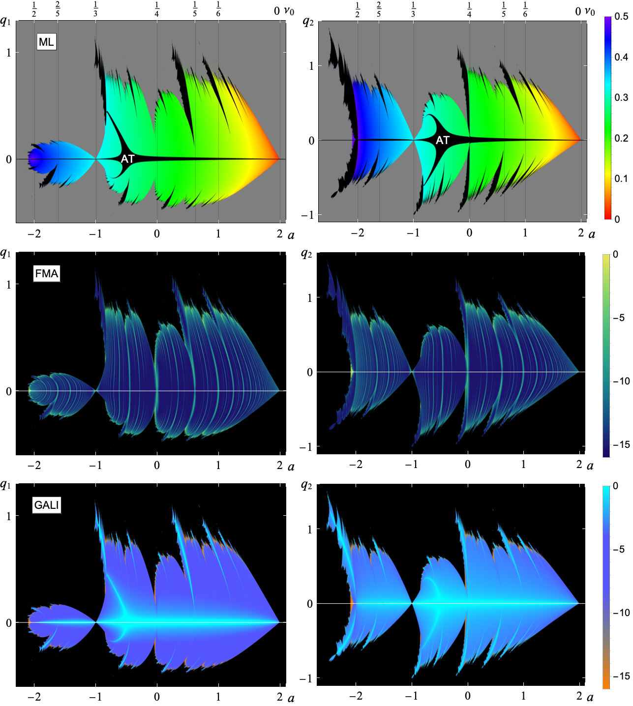
Figure 6: Isochronous and Period-doubling diagrams. The left and right columns display stability diagrams along the first $l_{1}$ (isochronous) and second $l_{2}$ (period-doubling) symmetry lines, respectively. In each plot, the abscissa represents the transformation trace $a$ at the origin, while the ordinate corresponds to the horizontal coordinate along the symmetry line. Different rows present various indicators: rotation number with mode-locking (in black) (ML), frequency map analysis (FMA), and the generalized alignment index (GALI). Unstable orbits are shown in gray in the top plots and in black in the middle and bottom rows.

V Understanding the diagram

V.1 Circle map and mode-locking

Before diving into the detailed analysis of our stability diagrams, it’s useful to revisit a specific dynamical system from the family of circle endomorphisms introduced by V. Arnold Givental et al. (2009); Boyland (1986); Ivankov and Kuznetsov (2001). This system is often employed to explore how intrinsic variables, such as the rotation number, change with system parameters, providing a foundational understanding that will support more advanced generalizations. Additionally, as will be seen in the final section, it has a direct connection to a particular case study of the Chirikov map.

The standard circle map is a one-dimensional transformation of a circle onto itself:

$$\mathrm{T}_{\nu_{0},\epsilon}:\,\theta^{\prime}=\phi(\theta)\mod 2\pi,\qquad\qquad\theta\in\mathbb{S}^{1}=[0;2\pi),$$

where the map is computed modulo $2\pi$, and the iterative function or two parameters is defined as:

$$\phi(\theta)=\theta+\Omega+\epsilon\,\sin{\theta},\qquad\qquad\Omega=2\,\pi\,\nu_{0}.$$ (13)

Here, $\nu_{0}\in[0;1)$ represents the bare/natural rotation number of an oscillatory system, while $\epsilon>0$ corresponds to the coupling strength, describing the level of externally applied nonlinearity.

By analyzing the behavior of $\phi(\theta)$, we can identify key scenarios depending on the value of $\epsilon$, with Fig. 7 providing a visual representation:

$\bullet$ Unperturbed case, $\epsilon=0$. The system exhibits a rigid rotation:

$$\theta^{\prime}=\theta+\Omega,$$

where every point moves at a constant angular velocity, $\Omega$. This motion is non-chaotic and highly regular, with the rotation number equal to $\nu_{0}$. For rational values of $\nu_{0}=p/q\in\mathbb{Q}$, the orbit completes $p$ full rotations around the circle exactly after $q$ iterations, forming a $q$-cycle. For irrational values of $\nu_{0}$, the motion is quasiperiodic, gradually covering the circle densely over time without ever repeating in a strictly periodic pattern.

$\bullet$ Small perturbations, $0<\epsilon<1$. In this range, the function $\phi(\theta)$ remains monotonically increasing (green curve in Fig. 7), meaning all orbits have to move forward. The map $\mathrm{T}_{\nu_{0},\epsilon}$ is an analytic diffeomorphism — smooth, invertible, and differentiable (along with its inverse) transformation. This case is particularly interesting to us, as it provides a qualitative framework for interpreting our diagrams.

$\bullet$ High perturbations, $\epsilon>1$. When $\epsilon$ exceeds 1, the function $\phi(\theta)$ is no longer bijective (as shown by the cyan curve in Fig. 7), making the circle map $\mathrm{T}_{\nu_{0},\epsilon}$ noninvertible. This opens the possibility to more complex dynamics, such as bistability and subharmonic routes to chaos.

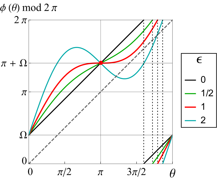
Figure 7: Standard circle map’s iterative function. The solid colored curves represent one period of the $\phi(\theta)\,\mathrm{mod}\,2\pi$ for different values of the coupling strength parameter $\epsilon=0,1/2,1,2$ as indicated in the legend. The red curve marks the critical case. The black dashed line corresponds to a linear function with a slope of 1, included for reference.

$\bullet$ Critical case, $\epsilon=1$. The value $\epsilon=1$ is referred to as critical, as it marks the boundary between two qualitatively different behaviors seen in the intervals $0<\epsilon<1$ and $\epsilon>1$. The map becomes an analytic homeomorphism of the circle, featuring a single cubic critical point where $\phi(\theta)$ is still continuous and invertible, but its inverse is no longer smooth (refer to red point/curve in Fig. 7).

In the space of the map’s parameters, for each orbit with initial condition $\theta_{0}$, the rotation number (if it exists) is given by the limit:

$$\nu=\frac{1}{2\,\pi}\,\lim_{n\rightarrow\infty}\frac{\phi^{n}(\theta_{0})-\theta_{0}}{n}.$$

The set of parameters corresponding to a given rotation number $\alpha$,

$$\mathcal{T}_{\alpha}=\{(\nu_{0},\epsilon)|\,\nu=\alpha\}$$

is known as the Arnold $\alpha$-tongue. For any fixed value of $0<\epsilon\leq 1$, the rotation number $\nu$ as a function of $\nu_{0}$ forms a continuous, non-decreasing curve known as the “devil’s staircase,” with flat steps of non-zero width at each rational value of $\nu$. These flat regions correspond to mode-locked states, where the dynamics are periodic, and the system is said to be “locked” to a specific rational rotation number. The boundaries of these regions are determined by algebraic curves satisfying the periodic condition for orbits with unit multipliers. Two examples of this staircase for $\epsilon=1/2$ (green) and $\epsilon=1$ (red) are shown in the top plot of Fig. 8. For $\epsilon=0$, the staircase degenerates into a linear function (black), with the flat segments disappearing entirely, as the set of rational numbers in the interval $[0,1]$ has a total measure of zero.

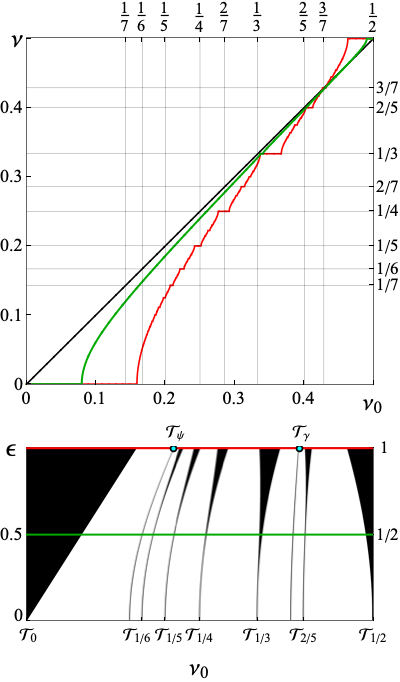
Figure 8: Arnold tongues. The top plot shows examples of devil’s staircases, where the rotation number $\nu$ is plotted against the bare tune $\nu_{0}$, with constant values of $\epsilon=1$ (red) and $\epsilon=1/2$ (green). The bottom plot schematically illustrates several Arnold tongues in the $(\nu_{0},\epsilon)$ space, shown in black. Rational tongues $\mathcal{T}_{\alpha}$ corresponding to mode-locking are labeled along the horizontal axis, where $\alpha$ matches the value of $\nu_{0}$. Two curves associated with irrational tongues, for $\psi=\sqrt[5]{2}-1$ and $\gamma=2-\phi$ (with $\phi$ as the golden ratio), are marked at the top, with terminal points indicated in cyan. The red and green lines link the devil’s staircases in the top plot to their corresponding parameter spaces below.

As $\epsilon$ increases, the measure of mode-locked states grows from zero to one, leading to a transition where quasiperiodic states become rare at $\epsilon=1$. At this critical point, the staircase becomes “complete,” meaning it is constant almost everywhere except on a Cantor set, with a fractal dimension of approximately $\approx 0.870$. This transition creates the familiar V-shaped regions, or rational tongues, in the parameter space, as shown in the bottom plot of Fig. 8. For a fixed value of $\epsilon$, rational tongues can be ordered by width, following a Farey sequence.

While rational tongues have an interior, tongues with irrational rotation numbers correspond to Lipschitz continuous curves connecting points $(\alpha,0)$ with $(\alpha_{t},1)$, where $\alpha_{t}$ is a terminal value. In the bottom plot of Fig. 9, two constant level sets of $\nu$ are shown for $\mathcal{T}_{\psi,\gamma}$, where $\psi=\sqrt[5]{2}-1$ and $\gamma=2-\varphi=(3-\sqrt{5})/2$ (with $\varphi$ being the golden ratio and the golden mean (GM) critical point at $\alpha_{t}\approx 0.607$).

For $\epsilon>1$, rational tongues may overlap, leading to complex behaviors such as bistability, where the system can exhibit two distinct stable states depending on the initial conditions, or period-doubling routes to chaos. Fig. 9 provides further details on these different dynamical regimes.

The top plot in Fig. 9 shows the parameter space, where the color represents the rotation number $\nu$ for initial conditions randomly selected from $\theta_{0}\in[0,2\pi)$. In contrast, the bottom plot uses additional black color to indicate mode-locked regions, offering a clear visualization of different dynamical regimes. The lower plot, with $\epsilon$ below the critical threshold, now offers a qualitative “zeroth-order” description of our diagrams in Fig. 6 for amplitudes below the resonance overlap, corresponding to the loss of stability. We will now explore the differences and proceed with a more detailed analysis.

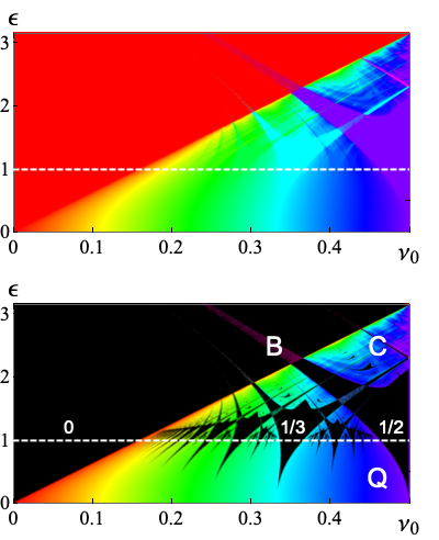
Figure 9: Dynamics of Circle map. The top plot shows the rotation number for the standard circle map across its parameter space $(\nu_{0},\epsilon)$, with $\nu$ evaluated for randomly chosen initial conditions $\theta_{0}$. The bottom plot classifies the dynamical regimes, marked with white labels. Black regions represent mode-locked states (some tongues are labeled with their corresponding rotation numbers), with “noisy” strips of constant color within these areas indicating regions of bistability (B). Colored points represent quasiperiodic motion (Q) for $\epsilon<1$ and chaotic motion (C) for $\epsilon>1$. The horizontal axis presents the color scale, since $\nu=\nu_{0}$ when $\epsilon=0$.

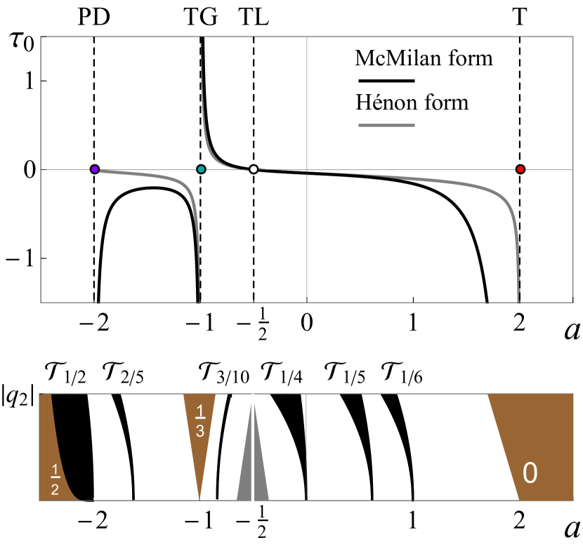
Figure 10: Hénon twists. The top plot shows the twist coefficient $\tau_{0}(a)$ for the Hénon quadratic map in both McMillan (black) and Hénon (gray) forms. The bottom plot schematically illustrates the structure of Arnold tongues along the second symmetry line, $l_{2}$, for small amplitudes ($q_{2}<0$). Regular tongues are shown in black, with the anti-tongue in gray. For remaining initial conditions, stable regions (both rational and irrational) are shown in white, while unstable regions (singular tongues) are marked in gold, with numbers indicating the resonance values of $\nu_{0}$ associated with instability.

V.2 Twisted tongues

When comparing the ML diagrams in Fig. 6 with the bifurcation diagram of the circle map Fig. 9, two qualitative differences stand out:

• Although rational tongues again appear in a sequence similar (but different) to the Farey sequence, for fixed values of $\nu_{0}=0$ and $\nu_{0}=1/3$ with small but nonzero distances along the symmetry lines ($|q_{1,2}|>0$), we observe instability rather than mode-locked motion — singular tongues. For $\nu_{0}=1/2$ (with $a=-2$), a pair of tongues $\mathcal{T}_{1/2}$ forms along the second symmetry line; however, the motion becomes unstable near the origin.

• Tongues respond differently to perturbations by varying slopes as a function of amplitude. For small $\epsilon$ in the circle map, the rotation number’s derivative with respect to $\epsilon^{2}$ varies monotonically

  $$\lim_{\epsilon\rightarrow 0}\mathrm{d}(2\,\pi\,\nu)/\mathrm{d}(\epsilon^{2})=-\frac{1}{4}\,\cot[\pi\,\nu_{0}].$$

  In contrast, for the quadratic Hénon map, with small $|q_{1,2}|$, tongues within $\nu_{0}\in(\nu_{\chi},1/3)$ ($-1<a<-1/2$) lean toward $\nu_{0}=0$, while otherwise they lean toward $\nu_{0}=1/2$.

Figure 10 very schematically depicts the Arnold tongue structure, with the vertical axis representing $|q_{2}|$ for $q_{2}<0$. Stable (rational and irrational) trajectories appear in white, while black regions indicate some mode-locked areas, and gold shows unstable initial conditions.

These differences can be understood through foundational works in dynamical systems and chaos theory, especially in the context of the Hénon map. We refer readers to relevant articles  Dullin and Meiss (2000); Dullin et al. (2000); Sterling et al. (1999) and their references for further detail, while we briefly summarize some key results here. According to the KAM theorem Kolmogorov (1954); Moser (1962); Arnold (1963), most invariant tori near a stable fixed point persist under small perturbations. This allows us to define the map’s canonical form as

$$\begin{array}[]{l}J^{\prime}=J,\\[7.11317pt] \theta^{\prime}=\theta+2\,\pi\,\nu(J),\end{array}$$

where $J$ is the action (or symplectic radius) and $\theta$ is the conjugate angle variables. In Birkhoff normal form theory (see, e.g.,Dullin et al. (2000)), the rotation number is often expressed as a power series of the action:

$$\nu(J)=\nu_{0}+\tau\,J=\nu_{0}+\tau_{0}J+\frac{1}{2!}\,\tau_{1}J^{2}+\frac{1}{3!}\,\tau_{2}J^{3}+\mathcal{O}(J^{4}),$$

where the derivative of $\nu$ with respect to $J$

$$\tau(J)=\frac{\mathrm{d}\nu}{\mathrm{d}J}=\tau_{0}+\tau_{1}J+\frac{1}{2}\,\tau_{2}J^{2}+\mathcal{O}(J^{3})$$

known as the twist, plays a critical role in nonlinear stability.

For the McMillan form mappings with a smooth, differentiable force function expandable around the origin as:

$$f(q)=a\,q+b\,q^{2}+c\,q^{3}+\ldots$$

the first twist coefficient, $\tau_{0}$, is expressed as:

$$2\,\pi\,\tau_{0}=\frac{1}{4-a^{2}}\,\left[4\,b^{2}\frac{a+1/2}{(a-2)(a+1)}-3\,c\right].$$ (14)

When $b\neq 0$, $\tau_{0}$ is defined for values of $\nu_{0}$ excluding $0,1/2$ and $1/3$ ($a\neq 2,-2,-1$), where it becomes singular, while $\tau_{1}$ also requires $\nu_{0}\neq 1/4,1/5,2/5$ ($a\neq 0,(-1\pm\sqrt{5})/2$). This result can be independently derived through various methods, such as Birkhoff normal forms Dullin et al. (2000), Lie algebra Bengtsson (1997); Morozov and Levichev (2017), square matrix method Yu (2017), Deprit perturbation theory Michelotti (1995), and, as recently shown, also extracted from related integrable McMillan multipoles Zolkin et al. (2024c, a), which offer additional qualitative insights. The top plot in Fig. 10 shows $\tau_{0}(a)$ for the quadratic Hénon map in both forms of the transformation.

When the rotation number of the stable fixed point reaches a rational value $m/n$ and the isoenergetic nondegeneracy condition $\tau_{0}\neq 0$ is met, KAM theory provides the following qualitative picture:

• For $n=1,2$ the fixed point loses linear stability when $|a|$ crosses 2. At $\nu_{0}=0$, the quadratic Hénon map undergoes a transcritical (T) bifurcation, while a cubic map undergoes a symmetric pitchfork (PF), creating an additional pair of fixed points. In Fig. 10, we see that $\tau_{0}$ is singular or zero at the period-doubling bifurcation (PD), depending on the from of the map. This difference explains why the fractal structure in the original Hénon map extends infinitely near $\nu_{0}=1/2$ while in the McMillan form it remains finite.

• For $n=3$, generally, the resonant term dominates the twist term near the origin, causing instability. In the quadratic Hénon map, this results in a touch-and-go (TG) bifurcation, while cubic or Chirikov mappings, due to additional spatial symmetry, stabilize with a symmetric pair of period-3 chains.

• For $n=4$ the origin may become unstable if the resonant term is sufficiently large.

• For $n>4$, the Moser Twist theorem implies stability of the fixed point, with bifurcations resulting in the creation of pairs of elliptic and hyperbolic $n$-cycles. Additionally, if $\tau_{0}=0$ and low-order resonances ($n\leq 6$) are absent, $\tau_{1}\neq 0$ provides a necessary stability condition Siegel and Moser (1971); Arnold (1988); Arnold et al. (2006).

When the twist vanishes at the fixed point, the stability condition becomes more complex, leading to what is referred to as a twistless (TL) bifurcations. As noted in Dullin and Meiss (2000), for the generalized Hénon map, assuming $n>6$ and $b\neq 0$, $\tau_{1}$ remains non-zero when $\tau_{0}=0$. From Eq. (14), we can understand the specific evolution of tongues around the origin, as well as why for the quadratic Hénon map we expect a twistless bifurcation at $a=-1/2$, which corresponds to the middle of the anti-tongue with an irrational rotation number:

$$\nu_{\chi}=\frac{1}{2\,\pi}\,\arccos[-1/4].$$

In contrast, the cubic map does not exhibit a TL bifurcation at $q=0$, because $\tau_{0}$ maintains a constant sign and never vanishes.

Figure 11 displays several rational and irrational tongues obtained by extracting constant level sets from the rotation number plots. Colored points and lines, mark singular bifurcations at the origin and represent unstable $n$-cycles, while the white point indicates the twistless bifurcation. The magnified plots (a and b.2) illustrate tongues for even ($\nu_{0}=1/6$) and odd ($\nu_{0}=1/5$) chains, revealing self-similar fractal structures resembling feathers, typical for higher-order resonances outside the positive twist region $a\in(-1,-1/2)$ (i.e., $\nu_{0}\in(\nu_{\chi},1/3)$).

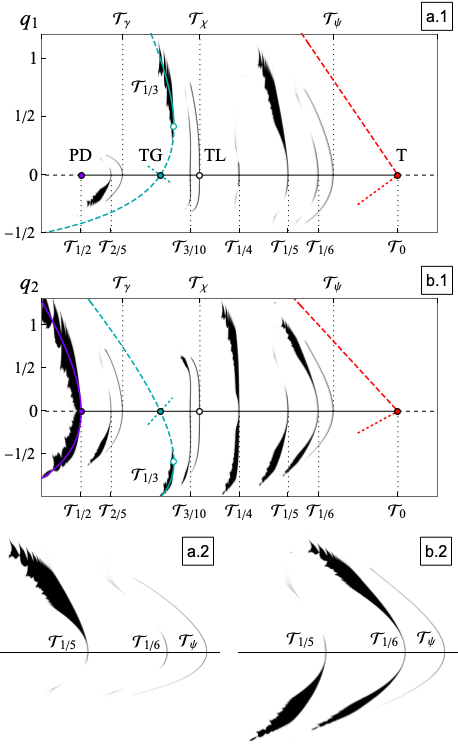
Figure 11: Feathers. Structure of Arnold tongues along the first (a.1) and second (b.1) symmetry lines for the quadratic Hénon map: rational tongues at $\nu_{0}=\frac{1}{2},\frac{1}{3},\frac{1}{4},\frac{1}{5},\frac{2}{5},\frac{1}{6}$, and $\frac{3}{10}$, and irrational tongues at $\nu_{0}=\psi,\gamma$, and $\chi$ (associated with the TL bifurcation). Singular and twistless bifurcations of the stable fixed point are indicated by points along the horizontal axis: transcritical (T), period-doubling (PD), touch-and-go (TG), and the creation of twistless torus (TL). Dashed lines depict the coordinates for the unstable fixed point (red), 2-cycle (purple), and 3-cycles (cyan, solid when stable). Dotted lines of the same colors indicate approximate locations of crossings with corresponding stable/unstable manifolds. The bottom plots magnify the vicinity of resonances at $\nu_{0}=1/5$ and $\nu_{0}=1/6$, highlighting the typical structures for odd and even island chains.

Notably, unlike the circle map, where every tongue near $|\epsilon|\approx 0$ is V-shaped, the situation differs here. As previously discussed, on one side of each symmetry line (for odd chains) or at both ends of one of the symmetry lines (for even chains), we encounter unstable nodes of the chain instead of crossing mode-locked islands. Consequently, for odd chains, the “feathers” are paired with lines, referred to as “cuts.” For even chains, two feathers or two lines appear together. In the next subsection, we will further investigate these crossings, while Figure 12 provides several phase space plots that visually support the diagrams in Figure 11.

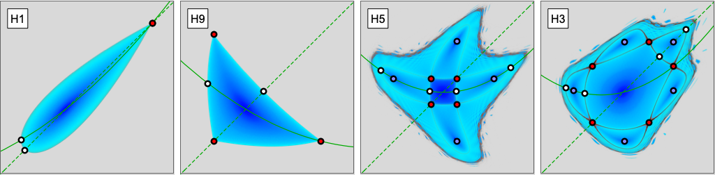
Figure 12: Symmetry lines and tongues. The first two plots show phase-space portraits near singular tongues corresponding to transcritical [H1] and touch-and-go [H9] bifurcations, where $\nu_{0}$ is close to 0 and 1/3. The following two plots represent typical scenarios for regular tongues, illustrating even [H5] and odd [H3] island bifurcations near $\nu_{0}=1/4$ and $\nu_{0}=1/5$. Stable cycles are shown in blue, unstable cycles in red, and intersections of symmetry lines with stable/unstable manifolds are highlighted in white. These phase-space portraits are recreations of Hénon’s original palettes (Fig. 2), presented here in McMillan form, with REM parameters used for coloring.

V.3 Tears and frays

Analyzing the rotation number along the symmetry lines, we observe a flat region when crossing an island center, similar to the behavior seen in the circle map (left plot in Fig. 13). However, at the node crossing, no mode-locking region appears, and the derivative of $\nu$ diverges to infinity (right plot).

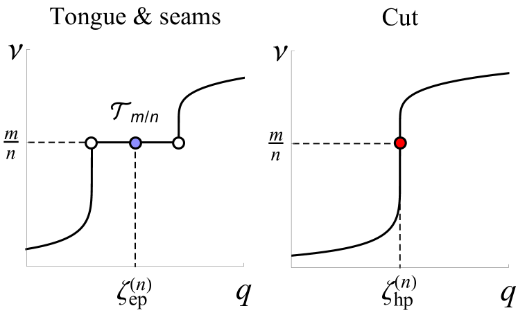
Figure 13: Seam and cut. Schematic illustration shows the devil’s staircase pattern as the symmetry line crosses through the center of the island (stable $n$-cycle $\zeta^{(n)}_{\text{ep}}$ in blue) and node (unstable $n$-cycle $\zeta^{(n)}_{\text{un}}$ in red). The left plot represents an Arnold tongue — a flat region bordered by intersections with the stable and unstable manifolds of $\zeta^{(n)}_{\text{un}}$ (white points). In the right plot, a “cut” appears where the derivative of $\nu(q)$ diverges to infinity.

As the system shifts toward chaotic behavior with overlapping resonances, the appearance of both tongues and cuts changes distinctly. To illustrate, we use an odd chain of 5 islands, chosen because it intersects both stable and unstable cycles on opposite sides of each symmetry line, making it convenient for study. The left plot in Fig. 14 shows two constant level sets, one for the rational tongue $\mathcal{T}_{2/5}$ and one for the irrational tongue $\mathcal{T}_{\gamma}$ along $l_{1}$, extracted with accuracies of $\delta\nu_{2/5}=3\times 10^{-4}$ and $\delta\nu_{\gamma}=8\times 10^{-5}$, respectively.

In the upper part of the plane (for $q_{1}>0$), the constant level set $\nu=2/5$ splits into two distinct sections: a “cut,” tracing an unstable 5-cycle (dashed orange line), which transitions into a “fray.” Both terms draw an analogy to tailoring, with the cut splitting the body of the main fractal. As the system transitions to chaos, this once fine line now resembles fraying fabric, with threads coming apart to form a loose edge. With increasing numerical precision, the cut narrows, exhibiting behavior characteristic of an irrational tongue, while the fray maintains its structure, showing chaotic orbits slowly wandering around the high-order resonances.

On the opposite side of the symmetry line, where $l_{1}$ crosses the middle of the island, the tongue takes on a wedge-like shape, similar to a dart often seen in sewing patterns. The middle of the dart represents the stable $5$-cycle (solid orange line), with edges attached to the main fractal by “seams,” much like two pieces of fabric sewn together. These seams mark the intersections of stable and unstable manifolds, forming an isolating separatrix that confines motion below the resonance overlap. When motion becomes chaotic, the seams detach from the main fractal, causing a “tear.”

The two plots on the right display the REM indicator for sections of the Hénon set near the tongue structure. Plot (a.) magnifies the fray, while plot (b.) reveals the seams and tears in the structure. In the chosen color scheme, gray represents unstable trajectories, red and dark shades indicate chaotic orbits, light blue highlights the cut and seam, and various shades of blue represent irrational KAM circles, with the color darkening around stable $n$-cycles. Palettes (c) show phase-space portraits for typical resonance stages: plot (c.1) and (c.2) showcase situation before and near resonance overlap, plot (c.3) illustrates strong overlap with some isolating invariant structures remaining, and plots (c.4,5) depicts the scenario where no invariant tori prevent escape. Finally, palettes (d.1–5) provide detailed magnifications of the island structure along the second symmetry line and its inverse, which mimics the opposite side of the tongue.

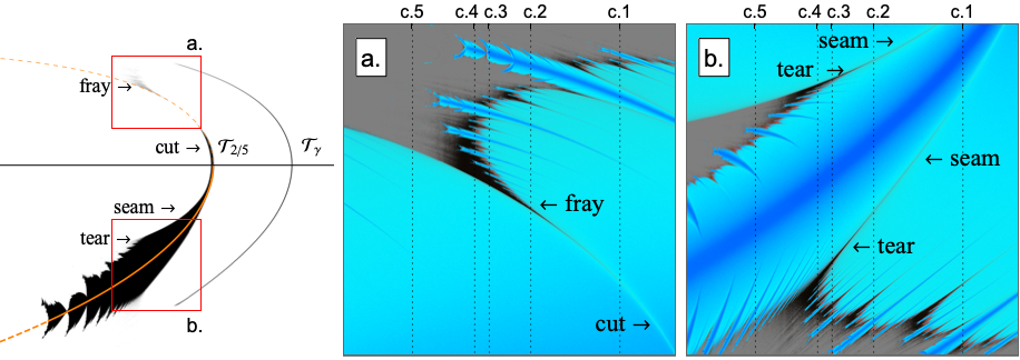
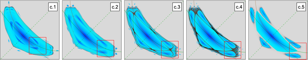
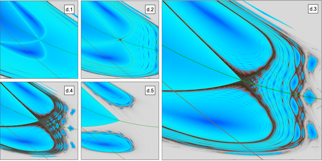
Figure 14: Tear and fray. Schematic illustration of the rational $\mathcal{T}_{2/5}$ and irrational $\mathcal{T}_{\gamma}$ Arnold tongues along the first symmetry line of the quadratic Hénon map. Points in black mark the level sets for these rotation numbers, determined with accuracies of $\delta\nu_{2/5}=3\times 10^{-4}$ and $\delta\nu_{\gamma}=8\times 10^{-5}$. Orange lines represent branches of the 5-cycle, shown as solid for stable and dashed for unstable. Insets (a.) and (b.) display REM indicators within the areas enclosed by red rectangles, highlighting features: seams and cuts in light blue, frays and tears in red/dark, rational and irrational rotations in shades of blue, and unstable regions in gray. Palettes (c.1–5) show phase-space diagrams and magnifications (d.1-5), illustrating typical stages in the destruction of invariant tori. Alongside the primary symmetry lines $l_{1,2}$ (green), a brown line represents the inverse symmetry $l_{2}^{-1}$, mirroring the crossing behavior on the opposite side of $l_{2}$.

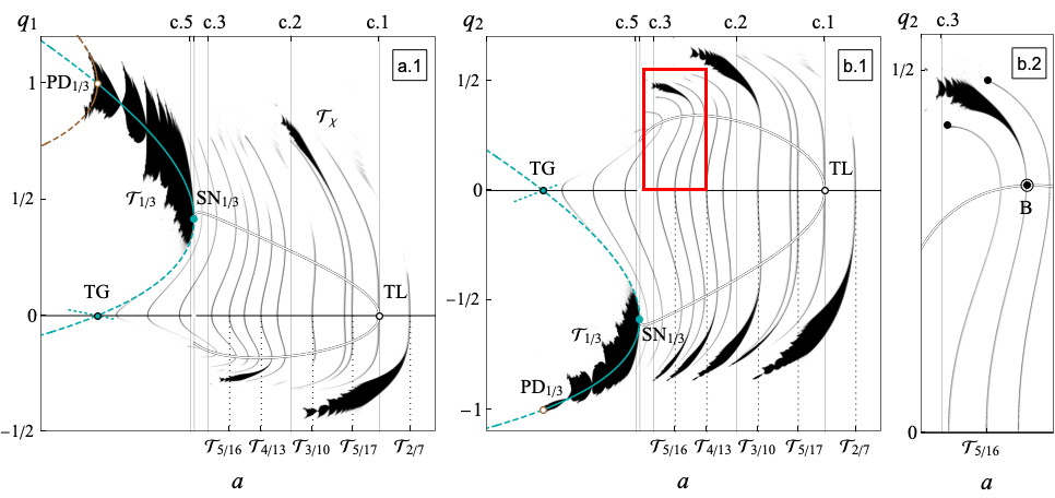
Figure 15: Ribcage and cobras. Structure of Arnold tongues in the Hénon map for the region with positive twist coefficient $\tau_{0}>0$, i.e., $a\in(-1,-1/2)$. Plots (a.1) and (b.1) highlight rational tongues along the first and second symmetry lines at $\nu_{0}=\frac{2}{7},\frac{5}{17},\frac{3}{10},\frac{4}{13},\frac{5}{16}$, and $\frac{1}{3}$; all other tongues, including $\mathcal{T}\chi$, represent irrational values of $\nu_{0}$. Colored points mark singular (TG) and twistless (TL) bifurcations at the origin and a saddle-node ($\text{SN}_{1/3}$) bifurcation where the twistless orbit (black/white curve) collides with stable and unstable 3-cycles (solid and dashed cyan curves). At $a=-1$, the stable 3-cycle undergoes a period-doubling bifurcation, producing a pair of stable 6-cycles (brown curve). The right plot (b.2) magnifies the red rectangle region in (b.1), detailing the rational tongue $\mathcal{T}_{5/16}$ and two irrational tongues (curves ending at terminal points). A bifurcation (B) occurs when a rational tongue intersects the twistless orbit. Markers at the top (c.1–5) indicate parameter values for corresponding phase-space diagrams and rotation number dependencies on $q_{1,2}$ (d.1–5), as provided in Fig. 16.

V.4 Twistless torus

We now shift our attention to the region with a positive twist coefficient, as illustrated in Fig. 15, which highlights several rational and irrational level sets of $\nu_{0}$. In this region, the rotation number becomes a non-monotonic function of amplitude, exhibiting a local minimum at the origin and maxima at the locations of the twistless orbit. This behavior causes the tongues to change the slopes of their boundaries, giving them a “cobra-like” appearance (see plot b.2) rather than the feather-like structure observed in Fig. 11. When a tongue crosses a twisted torus (marked by point B), higher-order bifurcations, such as saddle-node or reconnection bifurcations, are expected (for a detailed discussion, see Dullin et al. (2000)). Observing plots (a.1) and (b.1), the system resembles an X-ray of a fish: the twistless torus (depicted as the black/white curve) forms a “ribcage,” the fixed point at the origin acts as a backbone, and the surrounding tongues represent ribs. While twistless tori are generally associated with bifurcations, it appears to have a stabilizing effect in the Hénon quadratic map for moderate amplitudes. Within the region bounded by the twistless torus, tongues are significantly narrower (potentially lines), resulting in quasi-integrable dynamics. However, this stabilizing effect can be disrupted if the twistless orbit intersects major resonances, as will be discussed in the final section.

Tick marks at the top (c.1–5) correspond to phase-space portraits presented in Fig. 16, illustrating the evolution of the twistless orbit. Here, again, the REM indicator is used as a color scale: dark blue represents orbits near stable $n$-cycles and the twistless orbit itself (visible as a dark blue ring in palettes c.2 and c.3), light blue indicates less regular orbits, including unstable cycles and their manifolds, while red and dark colors represent chaotic trajectories.

At $a=-1/2$ ($\nu_{0}=\chi\approx 0.290$), a stable (since $\tau_{1}\neq 0$) twistless bifurcation occurs, see palette (c.1). As $a$ decreases, a twistless torus detaches from the origin (c.2), corresponding to an orbit with a local maximum in the rotation number. The bottom rows (d.1–5) complement the phase-space diagrams by providing rotation number plots $\nu(q_{1,2})$. Discontinuities and noise at larger amplitudes indicate instability and chaos.

As $a$ approaches $2-2\sqrt{2}$, the twistless orbit deforms (c.3) and develops a cusp at $\nu_{0}\approx 0.318$ (c.4). The cusp consists of a single parabolic 3-cycle and its associated manifolds. This configuration eventually breaks into a pair of stable and unstable 3-cycles (c.5) in a saddle-node bifurcation ($\mathrm{SN}_{1/3}$). At $a=-1$ ($\nu_{0}=1/3$), the stable cycle loses stability via a period-doubling ($\mathrm{PD}_{1/3}$) bifurcation, while the unstable cycle undergoes a touch-and-go (TG) bifurcation, passing through the origin and inducing instability at the resonance.

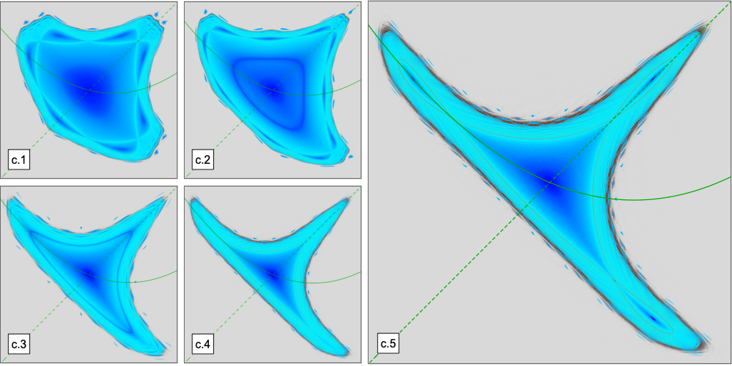
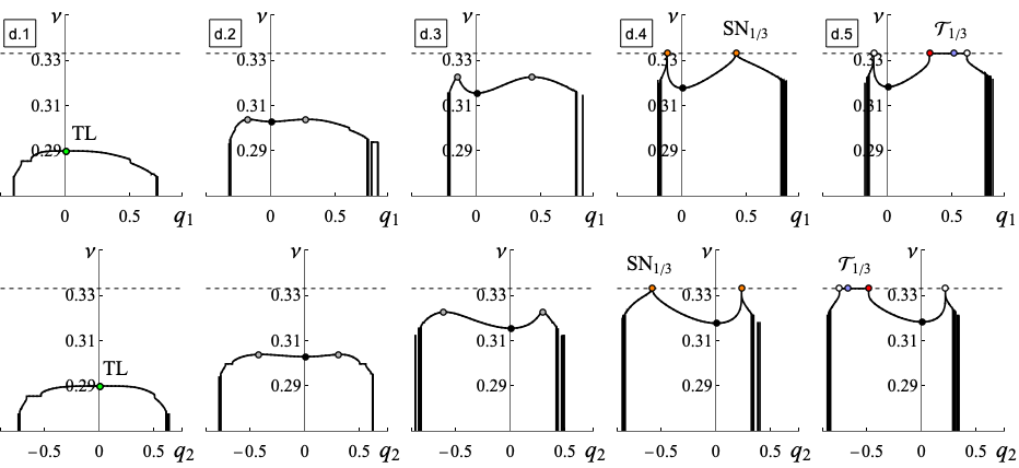
Figure 16: Evolution of the twistless orbit. The top group of plots shows phase-space portraits at different stages of the twistless orbit’s evolution (see Fig. 15 for further details): its birth at the origin in a twistless (TL) bifurcation (c.1), separation from the origin (c.2), just before cusp formation (c.3), annihilation in a saddle-node ($\text{SN}_{1/3}$) with a pair of 3-cycles (c.4), and the subsequent formation of 3 islands (c.5). Before bifurcation, the orbit is shown in dark blue, shifting to light blue at $\nu_{0}=1/3$. The bottom rows of plots (d.1–5) show rotation number dependencies along both symmetry lines (solid and dashed green curves). Colored points mark the twistless orbit (gray), the cusp orbit (orange), and stable and unstable 3-cycles (blue and red, respectively).

Examining the rotation number plots, we observe that as the system approaches the saddle-node bifurcation (d.3), the twistless orbit approaches $\nu_{0}=1/3$, creating a cut and seam around the origin, marked with orange points (d.4). After the saddle-node bifurcation ($a<-1$), one of the orange points (corresponding to the crossing of heteroclinic manifolds) remains as a cut in the vicinity of this parameter before transitioning into a fray. The other orange point evolves into a plateau corresponding to the regular tongue $\mathcal{T}_{1/3}$ (d.5); the blue and red points mark locations of stable and unstable 3-cycles respectively.

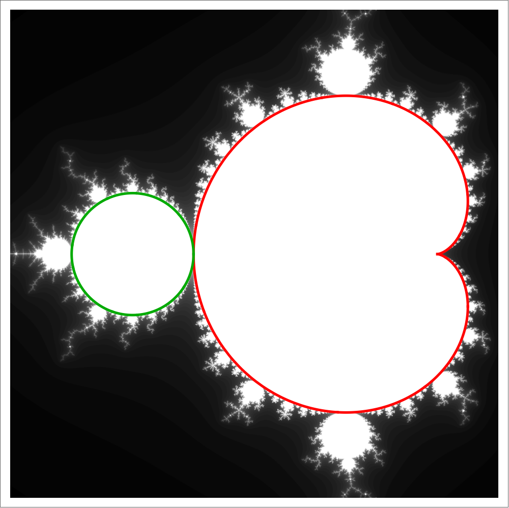
Figure 17: Elementary domains of the MBM set. The Mandelbrot-Brooks-Matelski set with its central cluster approximated by a cardioid (red) and a cluster at a non-root node approximated by a circle (green). Adapted from Dolotin and Morozov (2008).

V.5 Shapes of Elementary Domains

We began this section with a model problem: Arnold’s circle map. This 1D system provided valuable qualitative insights into the tongue structures near the origin. When combined with our understanding of twist behavior in symplectic maps, it also enabled reasonable quantitative estimates. However, as the system’s complexity increases, the circle map becomes insufficient for understanding the overall structure of the Hénon set, where critical amplitudes form complex geometries unlike the simple horizontal critical line at $\epsilon=1$.

In contrast, the MBM set offers another fractal structure with a nontrivial boundary. Remarkably, this boundary can be decomposed into elementary domains that are approximated with high precision by relatively simple equations. These domains take the form of cardioids at the cluster centers (the red curve in Fig. 17) or circles at the non-root nodes of the tree (green curves), respectively:

$$c-c_{0}=r_{0}\,e^{i\,\phi}\left(1-\frac{1}{2}\,e^{i\,\phi}\right)\quad\text{and}\quad c-c_{0}=r_{0}\,e^{i\,\phi}.$$

For further details, see Dolotin and Morozov (2008), which is dedicated to this analysis.

Similarly, we aim to explain the shapes of the “bulbs” that form the fractal body of the Hénon set. The top row in Fig. 18 illustrates the rotation number without mode-locking filtering. Here, unstable and chaotic orbits are rendered in black, making the shape of the set clearer.

Two distinct types of boundaries emerge to determine stability. “Ripped” boundaries, which arise from the overlap of island chains far from the system’s main resonances, define one type of stability limit. For the quadratic Hénon map, such regions include $a\in(0,1)$ or $a\in(-2,-1.5)$. These boundaries correspond to $\epsilon=1$ in the circle map but no longer align with any algebraic curve.

Resonance-driven boundaries, absent in the circle map, are linked to $\tau_{0}=0$ resonances and their associated singular tongues. Near resonances, these boundaries follow algebraic curves tied to unstable $n$-cycles (dashed lines in color). In integrable systems, these are the only type of boundaries (if any) in the parameter space that form well-defined bulbs (see plots b. and c.). Further from the resonance value of $\nu_{0}$, in chaotic systems the stability boundary deviates from the $n$-cycle.

To provide an alternative to $n$-cycle analysis, we now employ nonlinear integrable approximations. For the quadratic Hénon map, perturbation theory can be used to construct approximate invariants of motion that are conserved to a specified order of smallness parameter $\varepsilon$ (not to be confused with the circle map parameter $\epsilon$):

$$\mathcal{K}^{(n)}[p^{\prime},q^{\prime}]-\mathcal{K}^{(n)}[p,q]=\mathcal{O}(\varepsilon^{n+1}).$$ (15)

The invariant can be sought in the form of a polynomial:

$$\mathcal{K}^{(n)}=\mathcal{K}_{0}+\varepsilon\,\mathcal{K}_{1}+\varepsilon^{2}\,\mathcal{K}_{2}+\ldots+\varepsilon^{n}\,\mathcal{K}_{n},$$

where $\mathcal{K}_{m}$ consists of homogeneous polynomials in $p$ and $q$ of $(m+2)$ degree, with coefficients determined by satisfying the perturbation equation Eq. (15). Thorough discussion of this perturbation theory, along with higher-order analyses, will be provided in a subsequent publication. For now, the first two orders are covered in Zolkin et al. (2024c, a), with a summary of the essential points provided here.

Interestingly, the first two orders of this theory yield a general result

$$\begin{array}[]{l}\displaystyle\mathcal{K}^{(2)}[p,q]=p^{2}-a\,p\,q+q^{2}-\varepsilon\,\frac{b}{a+1}\,(p^{2}q+p\,q^{2})\,+\\[9.95863pt] \qquad\displaystyle+\,\varepsilon^{2}\left(\left[\frac{b^{2}}{a\,(a+1)}-\frac{c}{a}\right]p^{2}q^{2}\right)+\ldots\end{array}$$ (16)

that matches the integrable symmetric McMillan map. For the quadratic Hénon map,

$$f(q)=a\,q+q^{2},$$

the first- and second-order integrable approximations yield forces:

$$f_{\text{SX-1}}(q)=\frac{a\,(a+1)+q}{(a+1)-q}\,q=a\,q+q^{2}+\frac{q^{3}}{a+1}+\mathcal{O}(q^{4}),$$

and

$$f_{\text{SX-2}}(q)=\frac{a\,(a+1)+q}{(a+1)-q+\frac{1}{a}\,q^{2}}\,q=a\,q+q^{2}+\mathcal{O}(q^{4}).$$

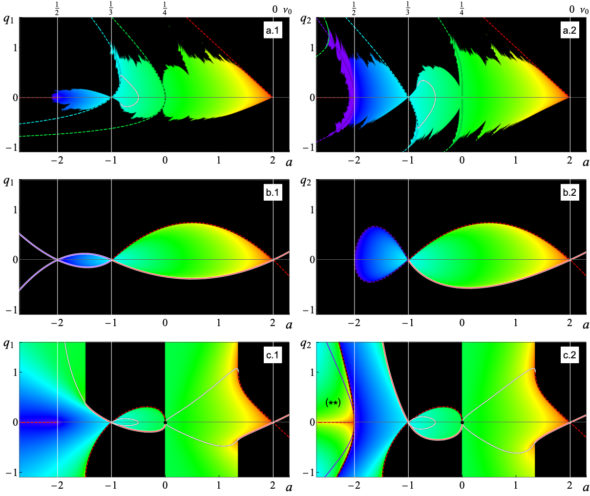
Figure 18: Approximate domains of the Hénon set. Hénon set (a.) compared to its integrable approximations using McMillan mappings in the first (b.) and second (c.) orders of perturbation theory. The bottom two rows show the rotation number evaluated in the simply connected regions around the origin and around the stable 2-cycle in the area marked with (**) in plot (c.2); otherwise, (**) area should be uniformly colored purple, indicating mode-locking within two islands. Solid and dashed lines represent stable and unstable $n$-cycles, colored according to their rotation numbers (red for fixed points, purple for 2-, cyan for 3-, and green for 4-cycles). The white line represents the coordinates of the twistless orbits. For plots (b.) and (c.), the white lines with color show the intersections with homo/heteroclinic connections.

The middle row of Fig. 18 illustrates the stability region for the SX-1 approximation. At this order, the motion is always bounded, resulting in two well-defined bulbs for $\nu_{0}<1/3$ and $\nu_{0}>1/3$. However, this order is insufficient to accurately match $\tau_{0}$ for the quadratic Hénon map and does not account for twistless orbits at the origin Zolkin et al. (2024c).

In the SX-2 order, $\tau_{0}$ is exactly matched Zolkin et al. (2024a). This approximation reveals a twistless orbit and additionally, it captures the formation of a bulb for $a\in(-1,0)$, corresponding to $\nu_{0}\in(1/4,1/3)$, as well as areas linked to $\mathcal{T}_{1/2}$ tongues for $a<-1/2$, marked with (**).

However, convergence becomes increasingly challenging in regions with ripped boundaries, where it is necessary to determine “the critical value of $\epsilon$” rather than relying on specific $n$-cycle coordinates. In the integrable approximation, for values of $a$ in the range $a\in(0,(-1+3\,\sqrt{57})/16)$ and $a<(-1-3\,\sqrt{57})/16$, unbounded motion around the origin is observed, signaling that the order of the approximation is insufficient to accurately capture the dynamics. Higher-orders reveal additional resonances, such as $1/5,\,2/5$, and $1/6$, but these models do not yield a well-defined integrable map, further complicating the analysis of the system’s behavior.

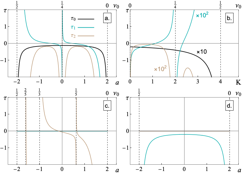
Figure 19: Twist. The first three twist coefficients are shown as functions of the parameter for various transformations in McMillan form: (a.) cubic map, $f_{+}(p)=a\,p+p^{3}$, (b.) Chirikov map, $f(p)=2\,p+\mathrm{K}\,\sin p$, (c.) fourth-power, $f_{+}(p)=a\,p+p^{4}$, and (d.) fifth-power, $f_{+}(p)=a\,p+p^{5}$, mappings. The scale at the top indicates the corresponding values of the bare rotation number, $\nu_{0}$. In plot (b.), additional scaling (shown in color) is utilized to improve the visual representation.

VI Results & Discussion

In this section, we present bifurcation diagrams for various mappings and discuss their key features and implications. By now, we assume the reader is familiar with interpreting these diagrams, particularly with the aid of the first twist coefficients. Figure 19 illustrates $\tau_{0}$ through $\tau_{2}$ for all mappings discussed. The scale at the top, labeled with values of the bare rotation number $\nu_{0}$, helps in identifying singularities, while the zero crossings of the lowest nonzero twist coefficient indicate the presence of twistless orbits.

VI.1 Hénon sets and sextupole magnet

A significant application of the quadratic Hénon map, in its original form Eq. (1), lies in modeling horizontal dynamics in accelerator lattices with thin sextupole magnets (see Zolkin et al. (2024c, a) for details). In this context, the variables $(x,y)$ represent normalized Floquet coordinates derived from the horizontal position $z$ and its longitudinal derivative, $\dot{z}=\mathrm{d}z/\mathrm{d}s$, where $s$ is the azimuthal coordinate of the accelerator ring Lee (2018).

Building on our prior explorations and following Hénon’s intent we conclude by presenting a final plot in the original form, Fig. 20, where we employ radius vectors along both symmetry lines, $r_{1,2}=\sqrt{x_{1,2}^{2}+y_{1,2}^{2}}$, instead of their projections, $x_{1,2}$, and use $\nu_{0}$ in place of the trace parameter, $a$. To reveal the internal structure of the tongues, the GALI indicator is used for coloring.

This plot holds critical experimental relevance, as it provides the dynamic aperture, which quantifies the stability of particles in the accelerator ring for given parameter settings. As noted earlier, the variation in scaling near $\nu_{0}=1/2$ compared to Fig. 6 is linked to the determinant of the Jacobian for the transformation (4) between different forms of the map. This connection can be further clarified with the insights provided by Fig. 10.

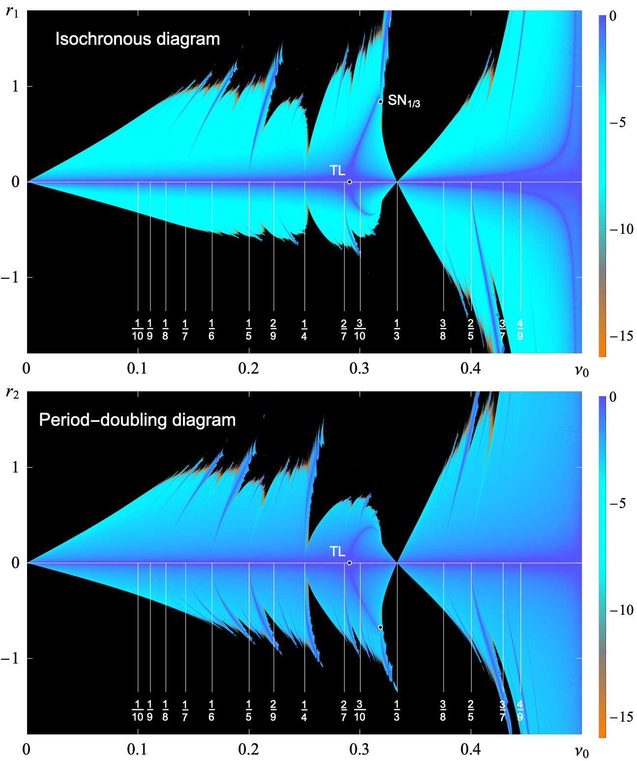
Figure 20: Hénon set. Isochronous and period-doubling diagrams for the Hénon map in its original form. The vertical axis represents the radial vector from the origin to the corresponding symmetry line, while the horizontal axis shows the bare rotation number. The generalized alignment index (GALI) is used for coloring.

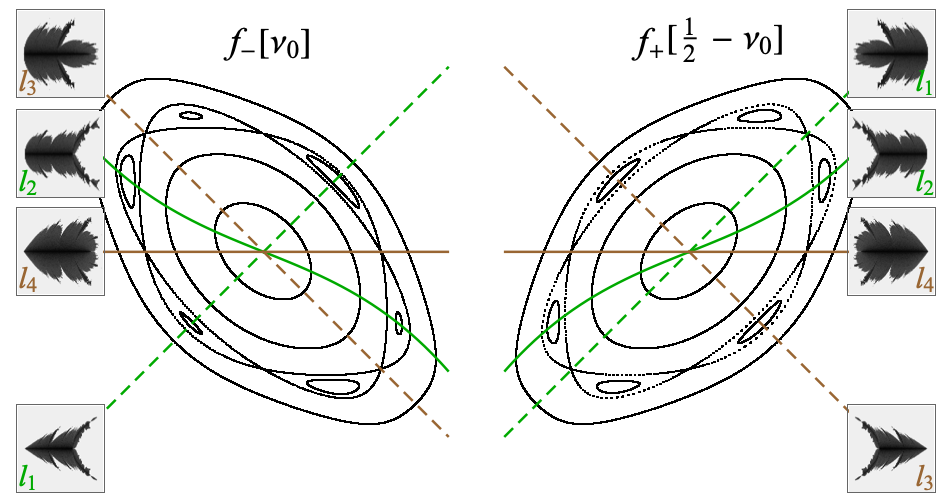
Figure 21: Odd force function. This figure illustrates the correspondence between phase space portraits and stability diagrams of the cubic mappings $f_{\pm}(p)=a\,p\pm p^{3}$, demonstrating the symmetry property $\nu_{0}\leftrightarrow\frac{1}{2}-\nu_{0}$. In this case, the chain of islands is formed by either two symmetric stable and two unstable 3-cycles (left) or a pair of stable and unstable 6-cycles. The first two symmetry lines, $l_{1,2}$, are depicted in green, while an additional pair of independent symmetry lines, $l_{3,4}$, is shown in brown. Stability diagrams for $f_{+}$ are presented in Fig. 22.

VI.2 Homogeneous Hénon mappings

In this Subsection we consider a family of mappings:

$$\mathrm{T}_{k}:\qquad\begin{array}[]{l}x^{\prime}=a_{1}\,x+b_{1}\,y+G_{k}(x,y),\\[7.11317pt] y^{\prime}=a_{2}\,x+b_{2}\,y+H_{k}(x,y),\end{array}$$

where $G_{k}$ and $H_{k}$ are homogeneous polynomials of degree $k>2$. Through similar reasoning as for the quadratic case, these mappings can be transformed into the form (1) with a single intrinsic parameter $\psi$ and a force function $F_{\pm}(x)=\pm x^{k}$. Just like the quadratic Hénon map, these mappings have physical interpretations in accelerator physics. They model rings with higher-order multipole magnets: octupoles ($k=3$), decapoles ($k=4$), and duodecapoles ($k=5$). The sign reflects the focusing or defocusing nature of the magnet. While octupolesGareyte et al. (1997); Leemann and Streun (2011); Plassard et al. (2021), alongside sextupoles, quadrupoles, and dipoles, are fundamental components of any modern accelerator, higher-order multipoles are increasingly used for advanced corrections in machine design Ohuchi et al. (2022).

To simplify the equations further, we apply transformation (3) and an additional isotropic scaling $(q,p)\rightarrow\varepsilon\,(q,p)$, where $\varepsilon^{k-1}\,\sin\psi=1$. This leads to a McMillan form mapping with

$$f_{\pm}(q)=a\,q\pm q^{k},\qquad a=2\,\cos\psi.$$ (17)

VI.2.1 Cubic Hénon map

As a specific example, we analyze the cubic transformations with $f_{\pm}(p)=a\,p\pm p^{3}$, representing a typical odd force function. For mappings in McMillan form that satisfy $f(p)=-f(-p)$, an additional spatial symmetry arises. Specifically, these mappings commute with the area-preserving involution:

$$\mathrm{T}=\mathrm{Rot}(\pi)\circ\mathrm{T}\circ\mathrm{Rot}^{-1}(\pi).$$

This property generates a distinct class of transformations:

$$\mathrm{Q}_{1}=\mathrm{Ref}(\pi/4)\circ\mathrm{Rot}(\pi)=\mathrm{Ref}(3\,\pi/4):\qquad\begin{array}[]{l}q^{\prime}=-p,\\[7.11317pt] p^{\prime}=-q,\end{array}$$

and

$$\mathrm{Q}_{2}=\mathrm{T}\circ\mathrm{Q}_{1}:\qquad\begin{array}[]{l}q^{\prime}=-q,\\[7.11317pt] p^{\prime}=p-f(q),\end{array}$$

which constitute an independent symmetry group, distinct from the one generated by $\mathrm{R}_{1}=\mathrm{Ref}(\pi/4)$ Roberts and Quispel (1992). As a result, the system exhibits two additional symmetry lines

$$\begin{array}[]{ll}l_{1}:\,p=q,&\qquad l_{2}:\,p=f(q)/2,\\[7.11317pt] l_{3}:\,p=-q,&\qquad l_{4}:\,p=0.\end{array}$$ (18)

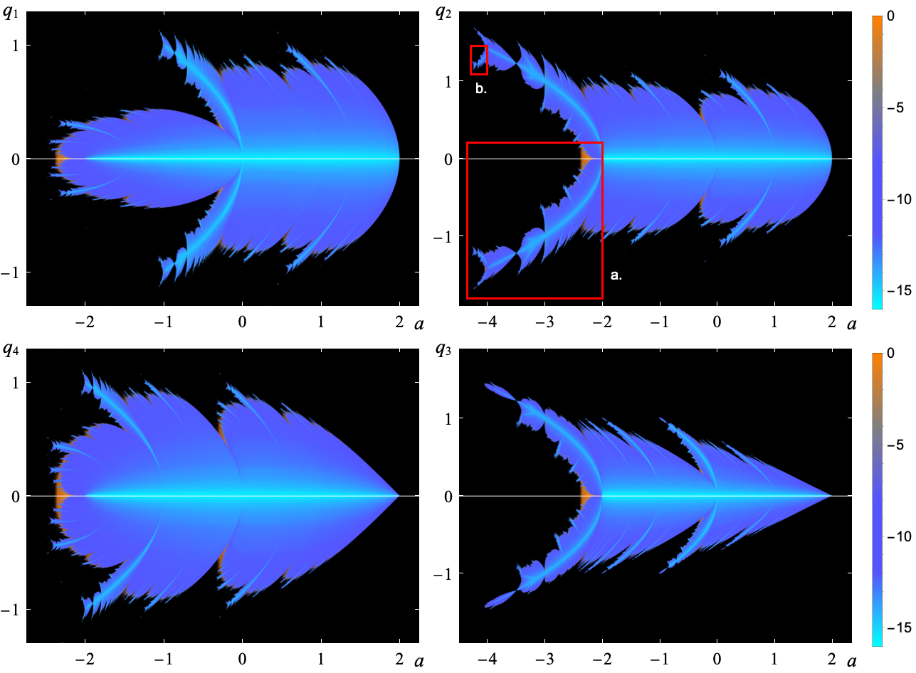
Figure 22: Beetles and Bugs. Stability diagrams (REM) for the homogeneous cubic map in McMillan form, $f_{+}(p)=a\,p+p^{3}$. The vertical axes represent the $q$ coordinate of points along the symmetry lines $l_{1,2,3,4}$. Fig. 23 compares areas (a.) and (b.).

While the presence of four distinct fractals adds some complexity to the interpretation, this is offset by the fact that the additional spatial symmetry simplifies the construction of stability diagrams (as the lower half $q<0$ of each fractal can be inferred using mirror symmetry), and that it suffices to analyze $f_{+}$, see Fig. 22. The fractals for $f_{-}$ can be reconstructed by simply reversing the direction of $a$ and swapping the indices of $l_{1}$ and $l_{3}$. An illustrative example is provided in Fig. 21. Additionally, when plotting rotation numbers, the color values must be transformed as: $\nu\rightarrow\frac{1}{2}-\nu,$ which can be readily understood as a consequence of Danilov theorem Nagaitsev and Zolkin (2020).

VI.2.2 Fourth and fifth power functions

Next, we present results for two additional mappings, characterized by the force functions

$$f(p)=a\,p+p^{4}\qquad\text{and}\qquad f(p)=a\,p+p^{5}$$

as shown in Figs. 24 and 25, respectively. These systems exhibit an atypical behavior, as they lack both lower-order terms $q^{2}$ and $q^{3}$. Consequently, the usual integrable approximation cannot be applied, and the first twist coefficient, $\tau_{0}$, vanishes for all $a\in(0,2)$. To gain insights into the slopes of resonance tongues and twistless orbits, it is necessary to consider $\tau_{1,2}$.

For instance, in plot (c.) of Fig. 19, we observe that the resonances at $\nu_{0}=\frac{1}{3},\,\frac{1}{5}$, and $\frac{2}{5}$ are singular, along with the emergence of three twistless bifurcations at the origin. Notably, only one associated anti-tongue is visible in Fig. 24, as the other two are too narrow in the parameter space to be easily discerned. Even this visible anti-tongue is barely distinguishable near the origin due to the weak dependence of amplitude on the rotation number. For $a>2$ in Fig. 24, the “trunk of an elephant” formation arises, representing the integer tongue $\mathcal{T}_{0}$ associated with the second fixed point

$$\zeta^{(1-2)}=\sqrt[3]{2-a}\times(1,1),$$

becoming stable as the origin loses stability at $a=2$.

Figure 23: Self-similarity. Magnified views of the regions highlighted by red rectangles in Fig. 22, showing self-similar structures after subtracting the corresponding coordinates of the 2-cycle (a.) or 4-cycle (b.).

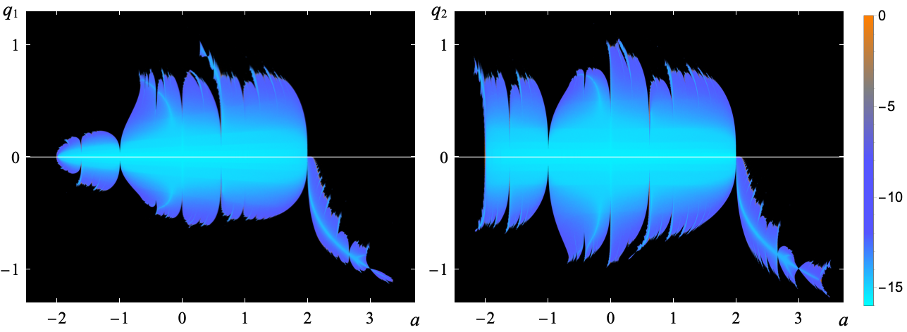
Figure 24: Elephant. Stability diagrams (REM) for the homogeneous fourth-power map in McMillan form, $f_{+}(p)=a\,p+p^{4}$. The vertical axes represent the $q$ coordinate of points along the symmetry lines $l_{1,2}$.

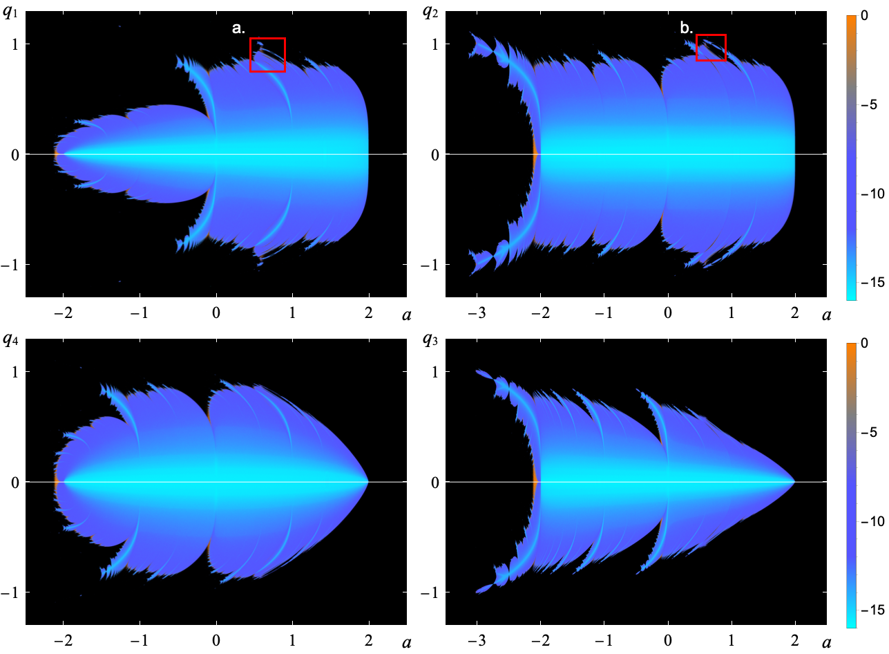
Figure 25: Hippo. Stability diagrams (REM) for the homogeneous fifth-power map in McMillan form, $f_{+}(p)=a\,p+p^{5}$. The vertical axes represent the $q$ coordinate of points along the symmetry lines $l_{1,2,3,4}$.

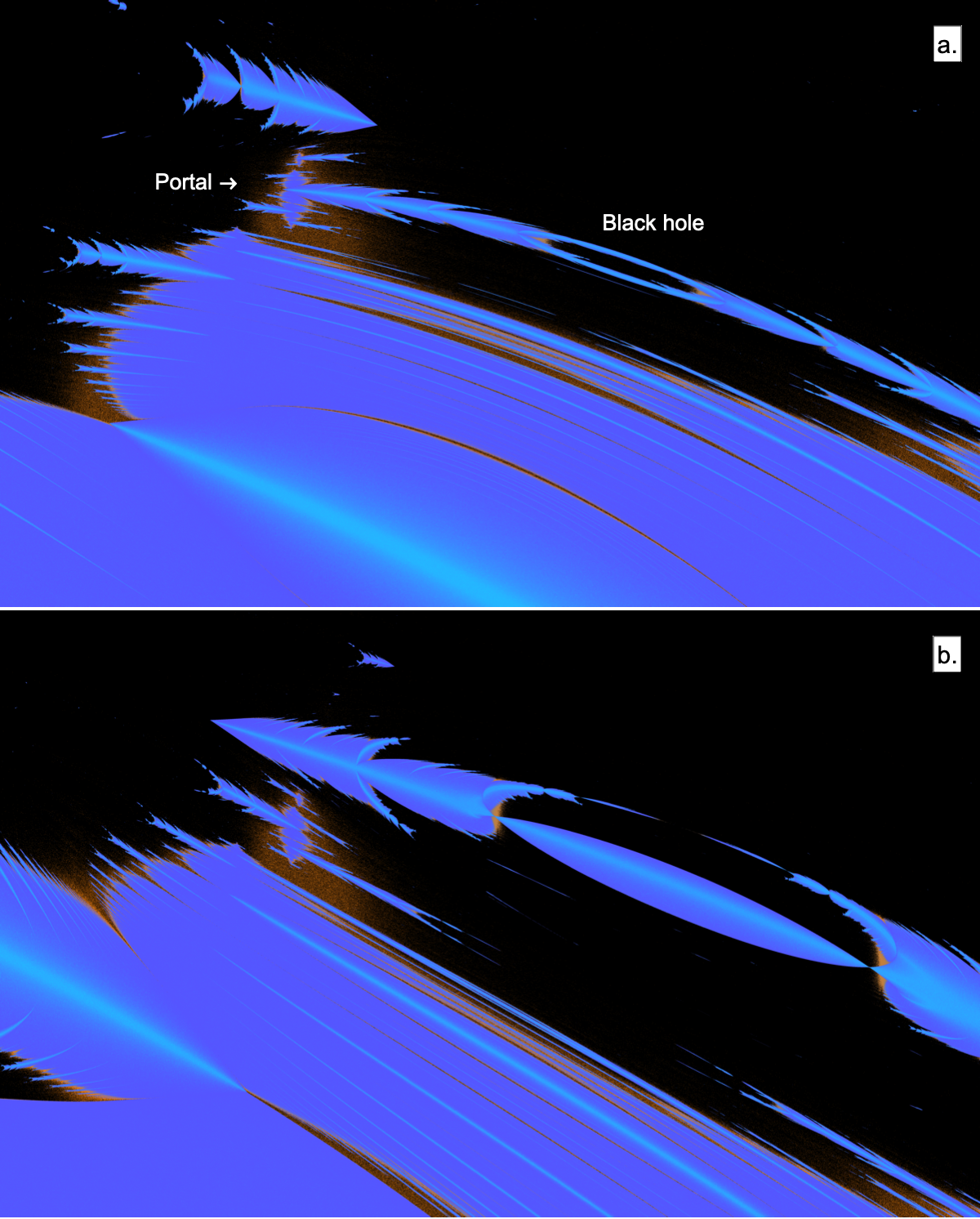
Figure 26: Portal and Black hole. Magnified views of the areas highlighted with red rectangles in Fig. 25.

In the fifth-power map, as with the cubic map, the first non-zero twist coefficient never vanishes. This implies the absence of twistless bifurcations at the origin; however, such bifurcations do occur within resonance tongues and are associated with higher-order ($n>1$) periodic orbits. Once again, four symmetry lines are required, and the overall fractal structure closely resembles that in Fig. 22.

At large amplitudes, the tongues exhibit highly complex overlap structures and bifurcations. To illustrate this, we provide magnified views of two regions from the top plots in Fig. 25, which might vaguely resemble the head of a hippopotamus. These magnifications are presented in panels (a.) and (b.) of Fig. 26.

While a detailed analysis of these systems is beyond the scope of this discussion, a few noteworthy observations can be made. In Fig. 26, we observe that distinct tongues can reconnect (as seen in the region labeled “black hole”), form intricate clusters (“portals”). Additionally, “splits” in the main body of a fractal that are filled wit chaotic trajectories (ca be seen in lower parts of both plots) undergo metamorphoses into higher-order tongues.

VI.3 Chirikov map

Next, we revisit the renowned Chirikov standard map Chirikov (1971, 1979), sometimes referred to as the Taylor-Greene-Chirikov map:

$$\mathrm{T}_{\mathrm{Chirikov}}:\qquad\begin{array}[]{l}I^{\prime}=I+F(\theta),\\[7.11317pt] \theta^{\prime}=\theta+I^{\prime},\end{array}$$ (19)

where $F(\theta)=\mathrm{K}\,\sin\theta$. Due to the periodicity of $F$, $\mathrm{T}_{\mathrm{Chirikov}}$ can be interpreted in three distinct settings: the plane $(\theta,I)\in\mathbb{R}^{2}$, a cylinder by taking $\theta\mod 2\pi$, or a torus by applying $\mod 2\pi$ to both equations. For additional details, refer to Zolkin et al. (2024b).

This map extends the circle map (13), which is obtained by setting $I^{\prime}=\Omega$ and $\mathrm{K}=\epsilon$ in the second equation. It also has direct applications in accelerator physics, particularly in describing longitudinal dynamics in machines with thin RF-stations, likely one of B. Chirikov’s original motivations.

Using the change of variables:

$$\begin{array}[]{ll}\theta=p,&\qquad q=\theta-I,\\[7.11317pt] I=p-q,&\qquad p=\theta,\end{array}$$ (20)

the Chirikov map can be expressed in McMillan form with

$$f(p)=2\,p+F(p),$$

and the trace of the transformation given by:

$$\operatorname{tr}\,\mathrm{d}\mathrm{T}_{\mathrm{Chirikov}}=2+\mathrm{K}\,\cos p.$$

The map has two fixed points, $(0,0)$ and $(\pi,\pi)$, which are stable under the respective conditions

$$-4<\mathrm{K}<0\qquad\text{and}\qquad 0<\mathrm{K}<4.$$

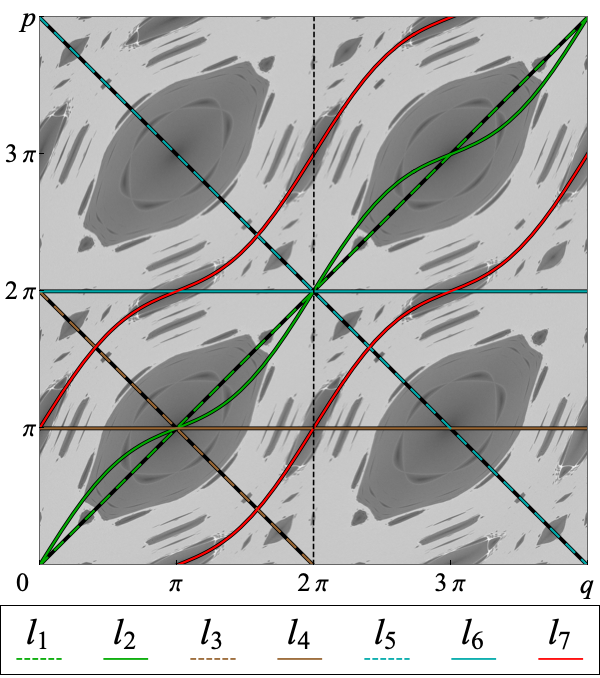
Figure 27: Symmetries of Chirikov map. Phase space diagram of the Chirikov map, showcasing the associated symmetry lines, color-coded as indicated in the legend.

The force function is odd with respect to both fixed points, as the map commutes not only with $\mathrm{Rot}(\pi)$, but also with a more general involution:

$$\begin{array}[]{l}q^{\prime}=-q+2\,\pi\,k,\\[7.11317pt] p^{\prime}=-p+2\,\pi\,k,\end{array}\qquad k\in\mathrm{Z}.$$

As a result, the map exhibits six symmetry lines, see Fig. 27:

$$\begin{array}[]{ll}l_{1}:\,p=q,&\qquad l_{2}:\,p=f(q)/2,\\[7.11317pt] l_{3}:\,p=2\,\pi-q,&\qquad l_{4}:\,p=\pi,\\[7.11317pt] l_{5}:\,p=-q,&\qquad l_{6}:\,p=0.\end{array}$$

Here, $l_{3}$ and $l_{5}$ are not independent, so the arithmetic quasiperiodicity of $f$ introduces only one additional symmetry line, compared to a generic odd force.

The map also commutes with a shift along the main diagonal $p=q$:

$$\mathrm{S}:\qquad\begin{array}[]{l}q^{\prime}=q+2\,\pi\,k,\\[7.11317pt] p^{\prime}=p+2\,\pi\,k,\end{array}\qquad k\in\mathrm{Z}.$$

This shift, though not an involution, represents an example of weak symmetry. The associated transformations $\mathrm{L}_{1}=\mathrm{R}_{1}\circ\mathrm{S}$ and $\mathrm{L}_{2}=\mathrm{T}\circ\mathrm{L}_{1}$, when considered $\mathrm{mod}\,2\,\pi$, introduce symmetry lines:

$$p=q+2\,\pi\,k\,\qquad\mathrm{and}\qquad l_{7,8}:\,p=\frac{f(q)}{2}\pm\pi.$$

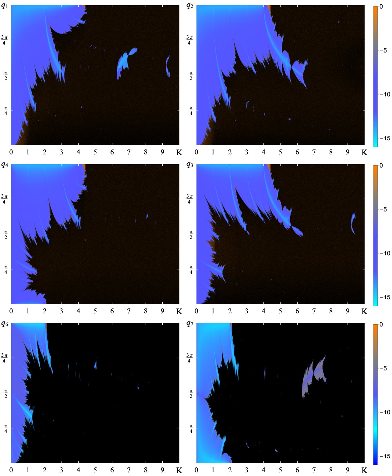
Figure 28: Chirikov map. Stability diagrams (REM) for the Chirikov map in McMillan form, $f(p)=2\,p+\mathrm{K}\,\sin p$. The vertical axes indicate the $q$-coordinates of points along the symmetry lines $l_{1,2,3,4,6,7}$, see Fig. 27 for reference.

Restricting to $\mathrm{K}>0$ (without loss of generality), only the fixed point at $(\pi,\pi)$ can be stable, with its rotation number given by:

$$\nu_{0}=\arccos(1-\mathrm{K}/2)/(2\,\pi).$$

Figure 28 shows the stability diagrams along the symmetry lines $l_{1,2,3,4,6,7}$, providing a comprehensive visualization of the map’s dynamical features. This concludes our exploration.

VI.4 Fracture of twistless structure

In addition to the diagrams in Fig. 22, the supplementary materials include three types of animations that explore additional aspects and raise intriguing questions. The playlist of animations, along with the corresponding code, is also accessible on YouTube and GitHub.

First, the videos labeled *_scan.mp4 demonstrate the correspondence between phase space portraits and stability diagrams, offering a dynamic perspective. Second, the animations titled *_rotation.mp4 showcase stability diagrams generated by rotating the cross-section $p=q$ instead of using a “true” symmetry line.

Finally, the most compelling animations, labeled *_mix.mp4, investigate the interplay of various parameter ratios, specifically $c/b$ and $c/d$. These animations reveal the evolution of twistless structures as the parameter $c$ is varied. For instance, when $b=0$, no twistless bifurcation occurs at the origin, but for the quadratic Hénon map $c=0$, the twistless structure appears as a unified entity in parameter space. However, as $c$ increases, the twistless structures evolve, eventually crossing major resonances and fracturing into multiple smaller segments. A detailed investigation into how the coherence of such structures is disrupted by various perturbations warrants a separate publication. As previously mentioned, while twistless orbits can stabilize dynamics at mid-range amplitudes, their influence can be overridden by the intrusion of higher-order tongues.

VII Summary

This study explores the visualization of dynamics in reversible symplectic mappings of the plane, focusing on the challenges posed by reducing the combined space of variables and parameters.

A dynamical system is reversible if there is an involution in phase space which reverses the direction of time. For discrete-time systems, this means the transformation is a composition of two distinct involutions, forming a group and defining two families of symmetries. Moreover, we demonstrate that groups of symmetric orbits arising from typical bifurcations of a fixed point, such as saddle-node, transcritical, period-doubling, $n$-island chain, and touch-and-go, can be identified along at least one of the two principal symmetry lines, addressing questions first posed in Hénon’s original work. To provide a more comprehensive description of these systems, the paper introduces the use of both isochronous and period-doubling diagrams, with the possibility of extending this framework in cases of multiple reversibility.

Modern chaos indicators, such as the Reversibility Error Method (REM) and the Generalized Alignment Index (GALI), are employed to analyze the dynamics further. These methods prove effective not only in identifying singular and mode-locked structures (Arnold tongues), but also in resolving twistless orbits and their associated bifurcations. Unlike isolated periodic $n$-cycles, which are governed by constant rotation numbers, twistless orbits follow a different intrinsic variable: zero twist, defined as the derivative of the rotation number with respect to the action variable. These orbits can represent quasiperiodic trajectories that densely fill closed curves in phase space.

This study provides both qualitative and quantitative analyses of fractal stability domains in the mixed parameter-symmetry line space, including approximations based on integrable McMillan maps. These methods are applied to practical problems, such as visualizing dynamic aperture in accelerator physics, which underscores their real-world relevance. For case studies, we analyzed systems representing longitudinal and transverse dynamics in accelerator lattices with various types of thin magnets and RF-station. We anticipate that a similar approach could be extended to other fields, such as addressing plasma stability in Tokamaks (see Chang et al. (2024)).

This research opens several intriguing avenues for further investigation. One compelling question concerns the existence of one-dimensional structures in phase space, analogous to symmetry lines, that intersect all asymmetric isolated $n$-cycles. Another is the potential universality and self-similarity of the observed diagrams. For instance, the Hénon-Heiles system — a model of planar stellar motion around a galactic center — upon phase space reduction yields a 2D mapping that exhibits striking structural similarities to the Hénon quadratic map Barrio and Wilczak (2020). Finally, as highlighted in the preceding section, the detailed dynamics of twistless orbits during interactions with primary resonances remain an open topic, presenting fertile ground for future exploration.

VIII Acknowledgments

The authors would like to thank Taylor Nchako (Northwestern University) for carefully reading this manuscript and for her helpful comments. This manuscript has been authored by Fermi Research Alliance, LLC under Contract No. DE-AC02-07CH11359 with the U.S. Department of Energy, Office of Science, Office of High Energy Physics. Work supported by the U.S. Department of Energy, Office of Science, Office of Nuclear Physics under contract DE-AC05-06OR23177. I.M. acknowledges that his work was partially supported by the Ministry of Science and Higher Education of the Russian Federation (project FWUR-2024-0041).

References

- Julia (1918) G. M. Julia, Journal de Mathématiques Pures et Appliquées 8, 47 (1918), [8e Série, Tome 1].
- Fatou (1917a) P. J. L. Fatou, Comptes Rendus de l’Académie des Sciences de Paris 164, 806 (1917a).
- Fatou (1917b) P. J. L. Fatou, Comptes Rendus de l’Académie des Sciences de Paris 165, 992 (1917b).
- Brooks and Matelski (1981) R. Brooks and J. P. Matelski, “The dynamics of 2-generator subgroups of PSL(2,),” in Riemann Surfaces And Related Topics: Proceedings of the 1978 Stony Brook Conference. (AM-97), Volume 97, edited by I. Kra and B. Maskit (Princeton University Press, Princeton, 1981) pp. 65–72.
- Mandelbrot (1980) B. B. Mandelbrot, Annals of the New York Academy of Sciences 357, 249 (1980).
- Hénon (1976) M. Hénon, Communications in Mathematical Physics 50, 69 (1976).
- Hénon (1969) M. Hénon, Quarterly of Applied Mathematics 27, 291 (1969).
- Gallas (1993) J. A. C. Gallas, Phys. Rev. Lett. 70, 2714 (1993).
- Sterling et al. (1999) D. Sterling, H. Dullin, and J. Meiss, Physica D: Nonlinear Phenomena 134, 153 (1999).
- Dullin and Meiss (2000) H. Dullin and J. Meiss, Physica D: Nonlinear Phenomena 143, 262 (2000).
- Dullin et al. (2000) H. Dullin, J. Meiss, and D. Sterling, Nonlinearity 13, 203 (2000).
- Inc. (2013) W. R. Inc., “Mathematica, version 10.0,” (2013), champaign, IL, 2013.
- Lewis Jr. (1961) D. C. Lewis Jr., Pacific Journal of Mathematics 11, 1077 (1961).
- DeVogelaere (1958) R. DeVogelaere, “IV. On the structure of symmetric periodic solutions of conservative systems, with applications,” in Contributions to the Theory of Nonlinear Oscillations (AM-41), Volume IV, edited by S. Lefschetz (Princeton University Press, 1958) pp. 53–84.
- McMillan (1971) E. M. McMillan, in Topics in modern physics. A Tribute to Edward U. Condon, edited by W. E. Brittin and H. Odabasi (Colorado Associated University Press, Boulder, CO, 1971) pp. 219–244.
- Roberts and Quispel (1992) J. Roberts and G. Quispel, Physics Reports 216, 63 (1992).
- Bazzani et al. (2023) A. Bazzani, M. Giovannozzi, C. E. Montanari, and G. Turchetti, Phys. Rev. E 107, 064209 (2023).
- Das et al. (2017) S. Das, Y. Saiki, E. Sander, and J. A. Yorke, Nonlinearity 30, 4111 (2017).
- Laskar (1999) J. Laskar, “Introduction to Frequency Map Analysis,” in Hamiltonian Systems with Three or More Degrees of Freedom, edited by C. Simó (Springer Netherlands, Dordrecht, 1999) pp. 134–150.
- Laskar (2003) J. Laskar, “Frequency map analysis and quasiperiodic decompositions,” (2003), arXiv:math/0305364 [math.DS] .
- Panichi et al. (2016) F. Panichi, L. Ciotti, and G. Turchetti, Communications in Nonlinear Science and Numerical Simulation 35, 53 (2016).
- Panichi et al. (2017) F. Panichi, K. Goździewski, and G. Turchetti, Monthly Notices of the Royal Astronomical Society 468, 469 (2017), https://academic.oup.com/mnras/article-pdf/468/1/469/11066230/stx374.pdf .
- Skokos et al. (2007) C. Skokos, T. Bountis, and C. Antonopoulos, Physica D: Nonlinear Phenomena 231, 30 (2007).
- Skokos and Manos (2016) C. H. Skokos and T. Manos, “The Smaller (SALI) and the Generalized (GALI) Alignment Indices: Efficient Methods of Chaos Detection,” in Chaos Detection and Predictability, edited by C. H. Skokos, G. A. Gottwald, and J. Laskar (Springer Berlin Heidelberg, Berlin, Heidelberg, 2016) pp. 129–181.
- Zolkin et al. (2024a) T. Zolkin, S. Nagaitsev, I. Morozov, S. Kladov, and Y.-K. Kim, “Dynamics of McMillan mappings III. Symmetric map with mixed nonlinearity,” (2024a), arXiv:2410.10380 [nlin.SI] .
- Chirikov (1971) B. V. Chirikov, “Research conserning the theory of non-linear resonance and stochasticity,” (1971), translated at CERN by A. T. Sanders from the Russian [CERN-Trans-71-40]. Nuclear Physics Institute of the Siberian Section of the USSR Academy of Science, Report 267, Novosibirsk, 1969 [IYAF-267-TRANS-E].
- Chirikov (1979) B. V. Chirikov, Physics Reports 52, 263 (1979).
- Turaev (2002) D. Turaev, Nonlinearity 16, 123 (2002).
- Zolkin et al. (2023) T. Zolkin, Y. Kharkov, and S. Nagaitsev, Phys. Rev. Res. 5, 043241 (2023).
- Zolkin et al. (2024b) T. Zolkin, Y. Kharkov, and S. Nagaitsev, Phys. Rev. Res. 6, 023324 (2024b).
- Barrio and Blesa (2009) R. Barrio and F. Blesa, Chaos, Solitons & Fractals 41, 560 (2009).
- Abraham and Marsden (1978) R. Abraham and J. E. Marsden, Foundations of Mechanics, 2nd ed., MSC: Primary 70; Secondary 37, Vol. 364 (Addison-Wesley Publishing Company, Inc., 1978) p. 826.
- Froeschlé et al. (1997) C. Froeschlé, R. Gonczi, and E. Lega, Planetary and Space Science 45, 881 (1997), asteroids, Comets, Meteors 1996 - II.
- Givental et al. (2009) A. B. Givental, B. A. Khesin, J. E. Marsden, A. N. Varchenko, V. A. Vassiliev, O. Y. Viro, and V. M. Zakalyukin, eds., “Small denominators. I. Mapping of the circumference onto itself,” in Collected Works: Representations of Functions, Celestial Mechanics and KAM Theory, 1957–1965 (Springer, Berlin, Heidelberg, 2009) pp. 152–223.
- Boyland (1986) P. L. Boyland, Communications in Mathematical Physics 106, 353 (1986).
- Ivankov and Kuznetsov (2001) N. Y. Ivankov and S. P. Kuznetsov, Phys. Rev. E 63, 046210 (2001).
- Kolmogorov (1954) A. N. Kolmogorov (1954) pp. 527–530.
- Moser (1962) J. Moser, Matematika 6, 51 (1962).
- Arnold (1963) V. I. Arnold, Russian Mathematical Surveys 18, 9 (1963).
- Bengtsson (1997) J. Bengtsson, The sextupole scheme for the Swiss Light Source (SLS): an analytic approach, Tech. Rep. SLS-TME-TA-1997-0009 (Paul Scherrer Institut, Villigen, Switzerland, 1997).
- Morozov and Levichev (2017) I. Morozov and E. Levichev, in Proceedings of the CERN-BINP Workshop for Young Scientists in Colliders, Geneva, Switzerland, 22 – 25 August 2016, CERN Proceedings, Vol. 1/2017, edited by V. Brancolini and L. Linssen (CERN, Geneva, 2017) pp. 195–206, CERN-Proceedings-2017-001.
- Yu (2017) L. H. Yu, Phys. Rev. Accel. Beams 20, 034001 (2017).
- Michelotti (1995) L. P. Michelotti, Intermediate Classical Dynamics with Applications to Beam Physics, Wiley Series in Beam Physics and Accelerator Technology (Wiley, 1995).
- Zolkin et al. (2024c) T. Zolkin, S. Nagaitsev, and I. Morozov, “Dynamics of McMillan mappings I. McMillan multipoles,” (2024c), arXiv:2405.05652 [nlin.SI] .
- Siegel and Moser (1971) C. L. Siegel and J. K. Moser, Lectures on Celestial Mechanics, 1st ed., Classics in Mathematics (Springer Berlin, Heidelberg, 1971).
- Arnold (1988) V. I. Arnold, Dynamical Systems III, 1st ed., Encyclopaedia of Mathematical Sciences (Springer Berlin, Heidelberg, 1988).
- Arnold et al. (2006) V. I. Arnold, V. V. Kozlov, and A. I. Neishtadt, Mathematical Aspects of Classical and Celestial Mechanics, 3rd ed., Encyclopaedia of Mathematical Sciences (Springer Berlin, Heidelberg, 2006).
- Dolotin and Morozov (2008) V. Dolotin and A. Morozov, International Journal of Modern Physics A 23, 3613 (2008), https://doi.org/10.1142/S0217751X08040330 .
- Lee (2018) S.-Y. Lee, Accelerator Physics, 4th ed. (World Scientific Publishing Company, 2018).
- Gareyte et al. (1997) J. Gareyte, J.-P. Koutchouk, and F. Ruggiero, Landau damping dynamic aperture and octupole in LHC, Tech. Rep. (CERN, Geneva, 1997) revised version number 1 submitted on 2003-08-21 14:12:02.
- Leemann and Streun (2011) S. C. Leemann and A. Streun, Phys. Rev. ST Accel. Beams 14, 030701 (2011).
- Plassard et al. (2021) F. Plassard, G. Wang, T. Shaftan, V. Smaluk, Y. Li, and Y. Hidaka, Phys. Rev. Accel. Beams 24, 114801 (2021).
- Ohuchi et al. (2022) N. Ohuchi, Y. Arimoto, K. Akai, K. Aoki, N. Higashi, K. Kanazawa, M. Kawai, T. Kawamoto, H. Koiso, Y. Kondou, M. Masuzawa, A. Morita, S. Nakamura, Y. Ohnishi, Y. Ohsawa, K. Oide, N. Okada, T. Oki, H. Sugimoto, M. Tawada, K. Tsuchiya, R. Ueki, X. Wang, H. Yamaoka, Z. Zong, B. Parker, M. Anerella, J. Escallier, A. Ghosh, H. Hocker, A. Jain, A. Marone, P. Wanderer, J. DiMarco, J. Nogiec, M. Tartaglia, and G. Velev, Nuclear Instruments and Methods in Physics Research Section A: Accelerators, Spectrometers, Detectors and Associated Equipment 1021, 165930 (2022).
- Nagaitsev and Zolkin (2020) S. Nagaitsev and T. Zolkin, Phys. Rev. Accel. Beams 23, 054001 (2020).
- Chang et al. (2024) C. Chang, S. Ku, R. Hager, J. Choi, D. Pugmire, S. Klasky, A. Loarte, and R. Pitts, Nuclear Fusion 64, 056041 (2024).
- Barrio and Wilczak (2020) R. Barrio and D. Wilczak, Nonlinear Dynamics 102, 403 (2020).