Sliding Squares in Parallel

Abstract

We consider algorithmic problems motivated by modular robotic reconfiguration, for which we are given $n$ square-shaped modules (or robots) in a (labeled or unlabeled) start configuration and need to find a schedule of sliding moves to transform it into a desired goal configuration, maintaining connectivity of the configuration at all times.

Recent work from Computational Geometry has aimed at minimizing the total number of moves, resulting in schedules that can perform reconfigurations in $\mathcal{O}(n^{2})$ moves, or $\mathcal{O}(nP)$ for an arrangement of bounding box perimeter size $P$, but are fully sequential. Here we provide first results in the sliding square model that exploit parallel robot motion, resulting in an optimal speedup to achieve reconfiguration in worst-case optimal makespan of $\mathcal{O}(P)$. We also provide tight bounds on the complexity of the problem by showing that even deciding the possibility of reconfiguration within makespan $1$ is -complete in the unlabeled case; for the labeled case, deciding reconfiguration within makespan $2$ is -complete, while makespan $1$ can be decided in polynomial time.

1 Introduction

Reconfiguring an arrangement of objects is a fundamental task in a wide range of areas, both in theory and practice, often in a setting with strong geometric flavor. A typical task arises from relocating a (potentially large) collection of agents from a given start into a desired goal configuration in an efficient manner, while avoiding collisions between objects or violating other constraints, such as maintaining connectivity of the overall arrangement.

In recent years, the problem of modular robot reconfiguration [8, 26, 28] has enjoyed particular attention [3, 1, 2, 4, 5] in the context of Computational Geometry: In the sliding squares model introduced by Fitch, Butler, and Rus [18], a given start configuration of $n$ modules, each occupying a quadratic grid cell, must be transformed by a sequence of atomic, sequential moves (shown in Figure 1(a)) into a target arrangement, without losing connectivity of the underlying grid graph. In the unlabeled version of the problem, all modules are identical, so only the shape of the arrangement matters; in the labeled variant, modules are distinguishable, and the location of individual modules has to be taken into account.

Aiming at minimizing the total number of moves, the mentioned previous work has resulted in considerable progress, recently establishing [2] universal configuration in $\mathcal{O}(nP)$ for a 2-dimensional arrangement of $n$ modules with bounding box perimeter size $\mathcal{O}(P)$, and $\mathcal{O}(n^{2})$ in three dimensions [1, 21]. However, the resulting schedules are purely sequential, not optimally minimizing the overall time until completion, called makespan. This differs from more practical settings, in which modules have the ability to exploit parallel motion to achieve much faster reconfiguration times—which is also a more challenging objective, as it requires coordinating the overall motion plan, not just at the atomic level (see Figure 1(b)), but also at the global level to maintain connectivity and avoid collisions.

(a) Two types of move can be performed by individual modules: (i) Slides and (ii) convex transitions.

(b) Some moves can be performed in parallel chain transformations, as shown here.

Figure 1: Our model allows for two types of moves to be chained into collision-free transformations. In this paper, we show the symmetric difference of a transformation using turquoise and yellow.

1.1 Our contributions

We provide first results for parallel reconfiguration in the sliding squares model with no restriction on the input. We achieve tight outcomes, both on the negative and the positive side.

1. We prove that the unlabeled version of parallel reconfiguration is -complete, even when trying to decide the existence of a schedule with the smallest possible makespan of $1$.

2. In the labeled variant, deciding makespan $2$ is -complete, while makespan $1$ is easy.

3. As our main algorithmic result for the unlabeled setting, we give a weakly in-place (see definition in Section 2) algorithm that achieves makespan $\mathcal{O}(P)$ where $P$ is the perimeter of the union of the bounding boxes of start and target configurations. This is not only a significant improvement over previous methods, it is also worst-case optimal, as there are straightforward examples in which this makespan is necessary.

Note that due to limited space, the majority of our proofs can be found in the appendix.

1.2 Related work

On the theoretical side, algorithmic methods for coordination the motion of many robots can be traced back to the classical work of Schwartz and Sharir [27] from the 1980s. On the practical side, Fukuda [19] presented an architecture for modular robots, followed by a wide spectrum of work that often used cuboids as elementary building blocks; see [31] for a survey.

Of particular interest for the algorithmic side is the sliding cube model (or square) by Fitch, Butler, and Rus [18], introduced in the context of a modular robotic hardware [8, 26, 28]. Recent work in Computational Geometry [13, 4, 1, 21] has studied algorithmic methods for sequentially sliding squares and cubes, with typical schedules requiring a quadratic number of moves. Also related are models with slightly different types of moves, such as “pivoting”, see [23, 9, 2, 3]. In [23] the authors claim an algorithm for connectivity-preserving reconfiguration of sliding squares in $\mathcal{O}(n)$ parallel steps. Unfortunately, this is incorrect for general input, requiring a forbidden local pattern (a $2\times 2$ arrangement with only two diagonally adjacent squares) to work, leaving the existence of linear-time parallel protocols unresolved. Similar models of parallel sliding squares have been investigated experimentally [29].

While this previous work on sliding squares focuses on minimizing the number of moves, a different line of research aims at minimizing the total time until completion. Hurtado et al. [20] studied parallel distributed algorithms for a less restrictive model of sliding square obtaining $\mathcal{O}(n)$ makespan. They show how to obtain the same result in the standard sliding square model using meta-modules, small groups of cooperating modules that behave like a single entity. This, however, imposes extra constraints in the input. Algorithmic research on meta-modules was considered in [5, 25]. In [6, 12], the authors considered coordinated motion planning for labeled robots to minimize the makespan, aiming for constant stretch, i.e., a makespan within a constant factor of the maximum distance for a single robot. This was extended to preserve connectivity for unlabeled [14, 7] and for labeled robots [17], and between obstacles [16]. These results are in a less constrained model than ours (see discussion in Section 2). Multi-robot motion planning was also at the focus of the 2022 CG:SHOP Challenge at SoCG; aiming at minimizing both the total number of moves and the makespan; see [15] for an overview, and [10, 30, 22] for outcomes.

2 Preliminaries

We study the discrete parallel reconfiguration of squares in the plane, particularly the infinite integer grid. Each simple $4$-cycle of edges in this grid bounds a unit cell, which can be occupied by up to one square module. A cell $u$ is uniquely identified by its minimal integer coordinates $x(u)$ and $y(u)$. Throughout this paper, we make use of cardinal and ordinal directions. In particular, the unit vector $(1,0)$ points east, $(0,1)$ points north, and their opposite vectors point west and south, respectively. For an illustration, see Figure 2(a). Two cells are edge-adjacent (resp., vertex-adjacent) if their corresponding squares share an edge (resp., vertex). If two cells are vertex-adjacent and not edge-adjacent, we call them diagonally-adjacent. A configuration $C$ of robots is defined by the set of occupied cells; we say that $C$ is valid if and only if its induced weak dual graph, defined as the cells’ edge-adjacency relation, is connected. Every configuration $C$ has a uniquely defined axis-aligned bounding box $B$ of minimal perimeter $P$ that contains it, see Figure 2(b).

We define the (open) neighborhood $N(c)$ of a cell $c$ as the set of cells that are edge-adjacent to $c$, and the closed neighborhood $N[c]$ as $N(c)\cup\{c\}$. Analogously, define $N^{*}(c)$ (resp., $N^{*}[c]$) as the open (resp., closed) neighborhood using vertex-adjacency. We abuse notation to express neighborhoods of sets of cells as $N[S]=\bigcup_{c\in S}N[c]$ and $N(S)=N[S]\setminus S$ (and analogously for vertex-adjacency).

(a) The integer grid $G$.

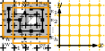
(b) A configuration of $n=10$ modules, its dual graph, and bounding box.

Figure 2: We illustrate the relation of the integer grid and configurations.

Individual modules can perform two types of move, slides and convex transitions, to travel into a different cell, see Figure 1(a). Both moves have local constraints; modules must exclusively slide along edges of adjacent cells that are continuously occupied, and convex transitions can only be performed through cells unoccupied both before and after the move.

When speaking of individual moves, we may denote them by their start and target cells, e.g., $u\rightsquigarrow v$. The parallel execution of legal moves constitutes a transformation. We assume that slides and convex transitions have equal duration, i.e., if started simultaneously as part of a transformation, they will also end simultaneously.

A transformation $C_{1}\rightarrow C_{2}$ is legal if it preserves connectivity and does not cause collisions, and a sequence of legal transformations is called a schedule. We define connectivity preservation based on connected backbones: Given a configuration $C$, we call a subset $M$ of modules free if $C\setminus M^{\prime}$ is a valid configuration for any $M^{\prime}\subseteq M$. Let $M\subset C_{1}$ refer to all moving modules during the transformation $C_{1}\rightarrow C_{2}$. Then there exists a connectivity-preserving backbone if and only if $M$ is free. A module $m$ is free if $\{m\}$ is free. In Figure 3, the first transformation is legal, the second does not have a connected backbone for every $M^{\prime}\subseteq M$, and the third attempts to use an illegal variant of the sliding move.

Figure 3: Disconnections in or from the backbone (marked modules) make transformations illegal.

We identify four types of collision, which we define as follows and illustrate in Figure 4.

1. Any two moves collide if their target cells are identical, or if they constitute a swap.

2. Two convex transitions collide if they share an intermediate cell (highlighted in red).

3. Two slides collide if one modules enters the cell that the other leaves, orthogonally.

4. A slide and a convex transition collide if the slide’s target cell is the start cell of the convex transition, and the latter starts in an orthogonal direction to the slide.

Figure 4: We illustrate examples of each collision type, (i)–(iv).

While collision types (i) and (ii) are motivated by the notion that a cell cannot fully contain two modules at once, the latter types are slightly more intricate. Recall that transformations occur fully simultaneously, so orthogonally conflicting directions as indicated in (iii) and (iv) are inherently infeasible as part of a single transformation.

Model comparison.

We note that our model is more constrained than already studied models for parallel reconfiguration under connectivity constraints [14, 17, 23, 20]. Michail et al. [23] do not explicitly require the connected backbone constraint, and do not explicitly define the collision model. The authors of [14, 17] consider a model that does not require the connected backbone constraint, and allows collision type (iii). Hurtado et al. [20] relax the free-space constraint of the slide move allowing a square to move through two diagonally adjacent static squares. They disallow chain moves as shown in Figure 1(b), so that the cells involved in individual slide moves in the same transformation are disjoint.

In parallel reconfiguration, it is commonly a desirable trait for all transformations to be reversible, which is now contradicted: an inverse transformation to (iv) is considered legal in our proposed model. To deal with this, we show the following.

Proposition 2.1.

A transformation that is illegal only because it contains collisions of type (iv) can be substituted by three legal, collision-free transformations.

This means that we can include transformations with collision type (iv) in algorithmic approaches and substitute them according to Proposition 2.1, obtaining schedules of comparable makespan. In addition, every transformation can now be reversed in constant time.

Problem statement.

We consider Parallel Sliding Squares, aiming for the connected reconfigurations of modules in the infinite integer grid by legal transformations, with an instance $\mathcal{I}$ composed of two configurations $(C_{1},C_{2})$ of $n$ modules. A schedule is feasible for $\mathcal{I}$ iff it transforms $C_{1}$ into $C_{2}$. The makespan of a schedule is the number of transformations in it. The decision problem for Parallel Sliding Squares asks, given an instance $\mathcal{I}$ and $k\in\mathbb{N}^{+}$, whether there exists a feasible schedule for $\mathcal{I}$ that has makespan at most $k$.

Throughout this paper, we use $B_{1}$ and $B_{2}$ to denote the bounding boxes of $C_{1}$ and $C_{2}$, respectively. We assume, as in the literature [24], that $B_{1}$ and $B_{2}$ share a bottom-left corner. A feasible schedule for $\mathcal{I}$ is in-place (as defined in [4, 24]) if and only if no intermediate configuration exceeds the union $B_{1}\cup B_{2}$ by more than one module. For technical reasons, we want dimensions of the bounding box that are multiples of three, and a three-wide empty column on the right of it. For that reason, we define an extended bounding box $B^{\prime}$ from the original bounding box $B$ of a configuration $C$. $B^{\prime}$ is obtained from $B$ by extending the right edge of $B$ to the right by three units, the left edge by one to three units, and the top (resp., bottom) edge by one or two units so that the dimensions of $B^{\prime}$ are multiples of three (see Figure 6). We say that a feasible schedule for $\mathcal{I}$ is weakly in-place if and only if intermediate configurations are restricted to the union of the bounding boxes extended by a constant amount. We refer to the standard definition of in-place as strictly in-place.

3 Computational complexity

We provide the following complexity result for Parallel Sliding Squares, which represents a complementary result to the -completeness result obtained by Akitaya et al. [4] for the sequential variant of this problem. This highlights a previously unrecognized gap in complexity when compared to closely related models for parallel reconfiguration under connectivity constraints. Most notably, Fekete et al. [14, 17] studied a related model and showed that deciding the existence of schedules of makespan $2$ is -complete, while makespan $1$ is in ¶.

Theorem 3.1.

Let $\mathcal{I}$ be an instance of Parallel Sliding Squares. It is -complete to decide whether there exists a feasible schedule of makespan $1$ for $\mathcal{I}$.

We reduce from the -complete problem Planar Monotone 3Sat [11], which asks whether a Boolean formula in conjunctive normal form is satisfiable. Each clause may consist of at most $3$ literals, all either positive or negative, and the clause-variable incidence graph must admit a plane drawing where variables are mapped to the $x$-axis, positive (resp., negative) clauses are mapped to the upper (resp., lower) half-plane, and edges do not cross the $x$-axis. Our reduction starts with a rectilinear embedding of the clause-variable incidence graph of an instance $\varphi$ of Planar Monotone 3Sat and constructs an instance $\mathcal{I}_{\varphi}$ of Parallel Sliding Squares using variable and clause gadgets. We then argue that $\varphi$ can be satisfied if and only if there is a single parallel transformation that solves $\mathcal{I}_{\varphi}$.

For a formula $\varphi$ over $m$ variables with $k$ clauses, we create $m$ copies of the variable gadget in a horizontal line, directly adjacent to one another. The literals in each monotone positive (negative) clause are then connected to by a clause gadget place above (below) the horizontal line of variables. A simple example of our construction is depicted in Figure 5(a).

(a) Our construction for $\varphi=(x_{1}\lor x_{3}\lor x_{4})\land(x_{1}\lor x_{2}\lor x_{3})\land(\overline{x_{1}}\lor\overline{x_{2}}\lor\overline{x_{4}})\land(\overline{x_{2}}\lor\overline{x_{3}}\lor\overline{x_{4}})$. The depicted transformations represent the satisfying assignment $\alpha(\varphi)=(\texttt{true},\ \texttt{false},\ \texttt{false},\ \texttt{false})$.

(b) Variable gadget (positive assignment).

(c) Clause gadget (monotone, positive).

Figure 5: An overview of our hardness reduction and the two types of gadget used.

Variable gadget.

The variable gadget consists of two empty circles of $20$ modules each, one containing an additional module in its interior, see Figure 5(b). These circles are connected by a solid, horizontal assignment strip of height $3$, to which individual clause gadgets are connected. While the gadget mostly retains its shape in the target configuration, the extra module must be moved from the interior of one circle to the other. There are two feasible transformations for this, representing a positive or negative value assignment.

Clause gadget.

The clause gadget consists of a thin horizontal strip that spans the gadgets of variables contained in the clause, and (up to) three vertical prongs that connect to the assignment strips of the incident variable gadgets. The structure, which is identical in both configurations of the instance, is depicted in Figure 5(c). Additionally, Figure 5(b) illustrates how the prongs connect clauses to variable gadgets.

Proof 3.2 (Proof sketch.).

Due to the way in which both configurations are connected, the schedule depicted in Figure 5(b) disconnects the variable gadget from either all its positive or negative clauses. Thus, a satisfying assignment maps to a feasible schedule. As these chain moves are unique schedules of makespan $1$, we also easily obtain the opposite direction.

Corollary 3.3.

The Parallel Sliding Squares problem is -hard: Unless $\P=\NP$, there is no polynomial-time $(1+\delta)$-approximation algorithm for $\delta\in[0,1)$.

4 A worst-case optimal algorithm

In this section, we introduce a four-phase algorithm for efficiently reconfiguring two given configurations into one another. Our approach computes reconfiguration schedules linear in the perimeter $P_{1}$ and $P_{2}$ of the bounding boxes $B_{1}$ and $B_{2}$ of $C_{1}$ and $C_{2}$, respectively.

Theorem 4.1.

For any instance $\mathcal{I}$ of Parallel Sliding Squares, we can compute a feasible, weakly in-place schedule of $\mathcal{O}(P_{1}+P_{2})$ transformations in polynomial time.

We also show that this is worst-case optimal:

Lemma 4.2.

The bounds achieved in Theorem 4.1 are asymptotically worst-case optimal.

The four phases of our algorithm concern themselves with (I) gathering $\mathcal{O}(P_{1})$ many modules to (II) construct a sweep-line structure, that is used to (III) efficiently transform the remaining configuration into an $xy$-monotone histogram. This histogram can then (IV) be transformed into any other $xy$-monotone histogram with the same number of modules, effectively morphing between the “start histogram” and the “target histogram”. To reach our target configuration, we then simply apply phases (I-III) in reverse. We refer to Figure 6 for a visualization of the different phases of the algorithm.

In the following subsections, we develop tools and give details of all phases that together yield a proof of Theorem 4.1; for details and the proof, we refer to Sections C.1 to C.6.

(a)

(b)

(c)

(d)

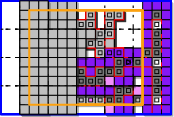
(e)

Figure 6: The high-level overview of our approach. (a) Initial configuration and (b–e) the result of Phases (I–IV), respectively.

4.1 Phase (I): Gathering squares

In Phases (I) and (II), we use an underlying connected substructure (called skeleton) of the initial configuration to guide the reconfiguration. Intuitively (formal definitions below), this tree-like skeleton functions as a backbone around which we move modules toward a “root” module, making a subtree “thick” (where the cells in the neighborhood of part of the skeleton are all full). This “thick” subskeleton is more “manipulable”, making it easier to mold it into a sweep line (Phase (II)). Moving modules around a tree is an idea also used by Hurtado et al. [20]. This type of strategy becomes complicated when the tree creates bottlenecks where potential collisions happen, which Hurtado et al. solves by strengthening the model and allowing the modules to “squeeze through” such bottlenecks. We achieve a stronger result in the classic sliding model via careful definition of the tree-like structure and move schedules.

Skeleton.

We define the skeleton of a configuration $C$ as a valid subconfiguration $S$ such that: $C\subset N[S]$ (every module of $C$ is either contained in $S$ or edge-adjacent to a module of $S$); and the dual graph of $S$ contains cycles of length at most 4, all of which are pairwise disjoint. We call a modules in $S$ (resp., $\notin S$) a skeleton (resp., nonskeleton) module. In Figure 6(a), skeleton modules are highlighted with an internal square and the perimeter of the skeleton is shown in red. Note that any set of nonskeleton modules is free.

We describe an algorithm to compute an skeleton $S$ from a given configuration $C$ in Section C.1. The main idea is to initially add to $S$ all modules with even $x$-coordinate, and modules with odd $x$-coordinate with no east and west neighbors. We then add more modules to $S$ to make it connected (highlighted with magenta squares in Figure 6(a)), but this might add large cycles to $S$. Finally, we break those cycles by removing modules from $S$ or exchanging them by another module in its neighborhood. By definition, contracting every cycle in $S$ renders a max-degree-4 tree where each node is either a cell or a 4-cycle. We refer to the nodes of this tree as nodes of $S$ and abuse notation by referring to $S$ as a tree.

Let $r$ be the root node of $S$, arbitrarily chosen. For every nonskeleton module, we arbitrarily assign an adjacent module in $S$ as its support. We define the subskeleton rooted at $c$ (denoted $S_{c}$) as the subconfiguration containing $c$ and its descendant nodes. The set $S_{c}^{*}$ contains the modules in $S_{c}$ and the nonskeleton modules supported by modules in $S_{c}$. The weight of a subskeleton $S_{c}$ is defined as $|S_{c}^{*}|$. By definition, $S_{r}^{*}=C$ and $|S_{r}^{*}|=n$.

Lemma 4.3.

Given a rooted skeleton $S$ and an integer $1<w\leq n$, there exist a node $c$ of $S$ such that $w\leq|S_{c}^{*}|\leq 3w$.

After computing $S$ we find a module $h\in S$ such that $|S_{h}|\in\mathcal{O}(P)$ using the above lemma (highlighted with a red inner square in Figure 6(b)). We then “thicken” $S_{h}$ into a structure we call exoskeleton.

Exoskeleton.

We define an exoskeleton $X_{c}$ as a reconfiguration of $S_{c}^{*}$ as follows. The core $\overline{X_{c}}$ of $X_{c}$ are positions in the lattice (no necessarily full) that form a subtree of $S_{c}$ containing $c$. Let $\mathcal{L}$ be the set of positions corresponding to the leaves of $\overline{X_{c}}$. We define $X_{c}$ in terms of $\overline{X_{c}}$:

1. $|\overline{X_{c}}|\geq 2$, and $X_{c}\subset N^{*}\left[\overline{X_{c}}\right]$. (All modules in $X_{c}$ are in the neighborhood of its core.)

2. $\mathcal{L}\cup\{c\}\subset X_{c}$. (The root and leaves are full.)

3. $N^{*}(\overline{X_{c}}\setminus\mathcal{L})\setminus\mathcal{L}\subset X_{c}$. (We call $N^{*}(\overline{X_{c}}\setminus\mathcal{L})\setminus\mathcal{L}$ the shell of $X_{c}$, shown in turquoise in Figure 7. The cells in the shell are full.)

4. The depth of every empty cell in $\overline{X_{c}}$ is a multiple of four.

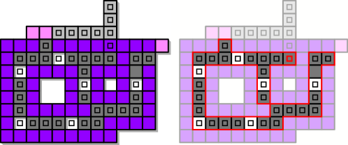
Figure 7: Exoskeleton. Skeleton and core cells are highlighted with a square. The right figure highlights the core of the exoskeleton. The root is highlighted with a red square.

The modules that are in $N^{*}(\ell)$, for a leaf $\ell\in\mathcal{L}$, and not in the shell or core of $X_{c}$ are called the tail modules of $\ell$ (shown in pink in Figure 7). Note that by definition, a module in $X_{c}$ either in the shell, in the core, or is a tail module. In all our figures we represent these modules in purple, dark gray, and pink, respectively. Intuitively, exoskeletons rely on their shell for connectivity since there are empty positions in their core. The empty positions are necessary to expand the exoskeleton making constant progress in constant time.

We prove by induction (Lemma 4.8) that we can reconfigure $S_{h}$ into an exoskeleton $X_{h}$ in $\mathcal{O}(P)$ transformations. Note that a minimal instance of an exoskeleton ($|\overline{X_{h}}|=2$) is a $3\times 3$ square of full cells. The base case of the induction is addressed in Corollary 4.5 below. In order to prove it, we need to show first how to handle skeletons lighter than 9 which we do in Lemma 4.4. This will also be important for our induction step. We call two connected subsets $S_{1}$ and $S_{2}$ of skeleton cells local if the subset of $S$ restricted to $N^{*}(S_{1}\cup S_{2})$ is connected. At first glance, the lemma might seem more complicated than it needs to, since without any obstacle, modules can freely move along the perimeter of $S$ (Figure 8(a)). However, extra caution is needed when multiple nonlocal pieces of the skeleton have already been converted to exoskeletons and those exoskeletons interact with the subskeleton $S_{c}$ we are currently processing: Note that modules in the working skeleton might be part of the shell of another exoskeleton (Figures 8(b–e)), making their movement dangerous (potentially disconnecting the nonlocal exoskeletons). We try leave such modules in their place, changing their membership from $S_{c}^{*}$ to the shell of the exoskeleton.

Lemma 4.4.

Let $C$ be a configuration with skeleton $S$ where potentially some of its subskeletons were reconfigured into exoskeletons. Let $c$ be a skeleton node such that $S_{c}$ is not yet part of an exoskeleton and $|S_{c}^{*}|\leq 9$, and let $d$ be its parent node. Let $M$ be the set of modules in $S_{c}^{*}$ that are not contained in exoskeletons. Then, within $\mathcal{O}(1)$ transformations, $M$ can be reconfigured so that:

• if $\deg(d)=2$, either $N^{*}[d]$ is full or $M\cap(N^{*}[c]\setminus N^{*}[d])$ is empty (i.e., the modules in $M$ are all contained in the neighborhood of $d$ if this region is not full);

• if $\deg(d)>2$, either $N^{*}[d]\cap N^{*}[c]$ is full or $M\cap(N^{*}[c]\setminus N^{*}[d])$ is empty (i.e., the modules in $M$ are all contained in the intersections of the neighborhood of $d$ and $c$ if this region is not full).

(a)

(b)

(c)

(d)

(e)

Figure 8: Illustration of Lemma 4.4. The boundaries of $N^{*}[d^{\prime}]$ and $N^{*}[c^{\prime}]$ are shown with dashed red and blue lines respectively.

By applying Lemma 4.4 (a constant number of times) in appropriate subskeletons we eventually obtain a solid $3\times 3$ square from which we can make an exoskeleton.

Corollary 4.5.

Given a subskeleton $S_{c}$ with $9\leq|S_{c}^{*}|$, we can reconfigure $S_{c}^{*}$ transforming one of its subskeletons into an exoskeleton in $\mathcal{O}(1)$ many transformations, without changing other exoskeletons or modules not in $S_{c}^{*}$.

For the inductive step we assume that we have a module $d\in S_{h}$ so that for every child $c$ of $d$, $S_{c}^{*}$ was reconfigured to an exoskeleton $X_{c}$. If $N^{*}[c]$ is full, we are done by making $c$ the root of the exoskeleton, effectively merging the children exoskeletons. Note that this will necessarily happen if $c$ had degree 4 and is not a 4-cycle. Thus, assume that there is an empty position $e\in N^{*}[c]$. We apply a routine Inchworm-Push that fills $e$ with local moves, using a module initially in the core of the exoskeleton $X_{c}$ (making that cell empty). We then a routine Inchworm-Pull to move core modules higher (in tree metric) which brings the empty positions down until they “exit” the exoskeleton at leaves. Again, without nonlocal interactions, we can rely on the shell for connectivity and these operations would be straightforward. However extra care is needed in the general case.

• Inchworm-Push: Let $c$ be a child of $d$, and $p$ be the parent of $d$. We branch into cases. (i) If $c$, $d$ and $p$ are collinear, there is a path $\pi$ in $N^{*}(d)$ from a child $c$ to $e$ going through only full cells (Figure 9(a)); (ii) If $c$, $d$ and $p$ form a bend, there is a path $\pi$ in $N^{*}(d)$ from $c$ to $e$ going through $d$ and at most one nonskeleton module (Figures 9(b–c)); (iii) In analogous cases to (i–ii), if a node in $\{c,d,p\}$ is a 4-cycle, there is a path $\pi$ in $N^{*}(d)$ from a module in $c$ to $e$ going through going through one module in the shell of $X_{d}$ (Figure 9(d)). For all cases, move the modules along $\pi$ making $e$ full and $d$ empty. This requires at most $2$ transformations since there is at most one collision along $\pi$ and we can decompose $\pi$ into two paths with no collisions.

  

  (a)

  

  (b)

  

  (c)

  

  (d)

  Figure 9: Inchworm-Push. Module $c$ is colored turquoise and cell $e$ is yellow.

• Inchworm-Pull: The operation happens in 5 stages, each composed of at most $2$ transformations. For every empty cell $p$ in the core, let $q$ be one of its children. In the first stage, if $q$ is not a leaf, move a module from $q$ to $p$. Figure 10(a) gives two examples, in one of which $p$ is a 4-cycle (that takes 2 transformations). If $q$ is a leaf, let $x(q)$ be its $x$-coordinate. Then, move a module from $q$ to $p$ in stage $j\in\{2,3,4,5\}$ if $x(q)\equiv j\,(\text{mod }4)$. If there is a tail module of $q$ that is originally in $S_{c}^{*}$ and not in another exoskeleton, move such a module to $q$ (Figures 10(b–c)). If there are no more tail modules we can update $\overline{X_{c}}$ by deleting $q$ which causes the tail module that just moved to become a shell module (Figure 10(b)), or causes two shell modules to become tail modules (Figure 10(c)).

(a)

(b)

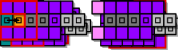
(c)

Figure 10: Inchworm-Pull. Module in cell $q$ is colored turquoise.

The following lemmas argue that these operations do not break connectivity and perform $\mathcal{O}(1)$ transformations. In Section C.2, we argue that even when Inchworm-Push moves modules in a nonlocal shell, we can use case analysis and Properties 3–4 of exoskeletons to establish connectivity locally (Figures 11(a–d)). In Inchworm-Pull many slide moves happen in parallel, and we have to argue connectivity with a global argument. In stage 1, we use Properties 3–4 to show that there is a cycle of modules that do not move surrounding the positions involved in the transformation (Figure 11(e)). For stages 2–5, if we moved all leaves simultaneously, local connectivity could be broken as shown in Figure 11(f). But the fact that we stagger the moves between 4 stages guarantee local connectivity.

Lemma 4.6.

Inchworm-Push maintains connectivity and takes $\mathcal{O}(1)$ transformations.

(a)

(b)

(c)

(d)

(e)

(f)

Figure 11: Inchworm operations preserve connectivity.

Lemma 4.7.

Let $X_{d}$ be an exoskeleton except for a potential violation of either Property 2, where the root $d$ might be empty, or Property 4, where the depth $(\text{mod }4)$ of all empty cells in $\overline{X_{d}}$ is a fixed $k\in\{1,2,3\}$. Then, Inchworm-Pull preserve connectivity and takes $\mathcal{O}(1)$ transformations.

Lemma 4.8.

Given a configuration $C$ with skeleton $S$, and a skeleton node $c$ with $|S_{c}^{*}|\geq 9$, a reconfiguration of $C$ transforming $S_{c}$ into an exoskeleton $X_{c}$ can be obtained in $\mathcal{O}(|S_{c}^{*}|)$ transformations.

Proof 4.9.

If a subskeleton of $S_{c}$ does not contain an exoskeleton, we can apply Corollary 4.5. If, after that, $S_{c}$ is not the core of an exoskeleton $X_{c}$, we apply induction. Let $Q$ be the set containing the children of $c$. For every child $q\in Q$ with $|S_{q}^{*}|\geq 9$ we can get an exoskeleton $X_{q}$ in $\mathcal{O}(|S_{q}^{*}|)$ transformations by inductive hypothesis. For every child $q\in Q$ with $|S_{q}^{*}|<9$, we apply Lemma 4.4 that either results in an exoskeleton $X_{q}$, or results in deleting $q$ from $S$ “compacting” all its modules in $N^{*}(q)\cap N^{*}(c)$. If after that $N^{*}(c)$ is not full, $N^{*}(h)$ contains at most 3 empty cells if $c$ is a degree-2 bend in $S$, at most 2 empty cells if $c$ is a “straight” degree-2 in $S$, or at most 1 empty cell if $c$ has degree 3. (Note that if $c$ has degree 4, then $N^{*}(c)$ is full.) For each of these empty cells, we can fill them by apply Inchworm-Push followed by at most 4 applications of Inchworm-Pull. Then, after $\mathcal{O}(1)$ transformations, by Lemmas 4.6, LABEL: and 4.7, $N^{*}(c)$ becomes full. If $N^{*}(c)$ is full, the configuration contains an exoskeleton $X_{c}$ except for the “4-arity” of the empty positions. That can be fixed by the application of Inchworm-Pull at most 3 times on $X_{c}$.

By Lemma 4.3, we can choose an appropriately heavy node $h$ of $S$ to obtain:

Corollary 4.10.

Let $C$ be a configuration with bounding box perimeter $P$. We can reconfigure $C$ so that it contains an exoskeleton with $\geq 36P$ modules in $\mathcal{O}(P)$ transformations. All modules stay within the extended bounding box of $C$.

4.2 Phase (II): Scaffolding

After obtaining a large enough exoskeleton $X_{h}$, we reconfigure it so that it contains a “T-shaped” exoskeleton containing the right edge of the extended bounding box. The vertical part of this “T” will be used as a “sweep line” in Phase (III). Phase (II) consists of 3 steps:

1. We first “compact” $X_{h}$ so that its core contains no empty cells.

2. We then choose a rightmost node $c$ in the core of $X_{h}$ and grow a horizontal path from that node rightward, until a $3\times 3$ square is formed outside the bounding box (Figures 12(a–f)).

3. Grow the path upwards until it hits the top of the bounding box, then grow a path downwards until it hits the bottom of the bounding box (Figures 12(f–h)).

We achieve these steps using Inchworm-Push and Inchworm-Pull by changing the root of the exoskeleton to $c$ (see Section C.3). We make sure that $X_{c}$ always contain $h$ and so that it is always connected with the subset of $S$ that was not transformed into an exoskeleton. We use the connectivity properties of exoskeletons to “go through” obstacles without breaking connectivity in Step 2 (Figures 12(a–f)). The only case in that we cannot use Inchworm-Push is when some module in the path $\pi$ is a cut vertex. In such a case, we sequentially fill in up to two cells in the neighborhood of $X_{c}$ (shown in yellow in Figure 12(b)), making all modules in $\pi$ noncut.

(a)

(b)

(c)

(d)

(e)

(f)

(g)

(h)

Figure 12: Building the scaffolding. The extended bounding box is shown in blue.

4.3 Phase (III): Sweeping into a histogram

Once Phase (II) concludes, we are left with an intermediate configuration $C$ that contains a highly regular scaffold configuration. Our goal in the remaining phases is to transform the entire configuration into meta-modules, small units of modules that cooperate to provide greater reconfiguration capability, that can then be used for efficient, weakly in-place reconfiguration.

Meta-module.

A meta-module with center cell $v$ is a configuration $M$ of at least eight modules such that $N^{*}(v)$ is full. This corresponds a clean “O”-shaped cycle of eight modules, or a solid $3\times 3$ square. We denote the cells in $B^{\prime}$ that share their $y$-coordinate with $M$ and have $x$-coordinates at least $x(v)+2$ by $\textsc{e}(M)$, and define $\textsc{w}(M)$ analogously, see Figure 13.

Figure 13: (a) A clean meta-module, (b) a solid meta-module, and (c) the east-/ west strips.

To build these meta-modules in an efficient, parallelized manner, we exploit the skeleton created during Phase (II), which we reconfigure into a sweep line.

Sweep line.

A configuration $C$ contains a sweep line exactly if it has a connected sub-configuration ${\ell}\subset C$ that spans the full height of its bounding box, composed of $h$ disjoint meta-modules $M_{1},\ldots,M_{h}$ that have center cells with a identical $x$-coordinates, $x({\ell})$. Let $v_{i}$ now refer to the center cell of $M_{i}$, such that $y(v_{i})<y(v_{j})$ exactly if $i<j$. We define the half-spaces $\textsc{e}({\ell})$ and $\textsc{w}({\ell})$ as the union of east and west strips, respectively.

We refer to a sweep line ${\ell}$ as clean exactly if every meta-module $M_{i}$ is either clean or has a fully occupied west strip, $\textsc{w}(M_{i})\subseteq C$. Analogously, if its meta-modules are all solid, so is ${\ell}$. Furthermore, we say that is ${\ell}$ a separator if for every meta-module $M_{i}$ in ${\ell}$:

1. The west strip $\textsc{e}(M_{i})$ does not contain modules unless all cells in $\textsc{w}(M_{i})$ are full.

2. The modules in $\textsc{e}(M_{i})$ are located in its $x$-minimal cells, thus forming a $3$ cell tall rectangle with at most two additional “loose” modules.

We start by transforming the scaffold at the east boundary of $B$ into meta-modules that can then cooperate to perform additional operations with the remaining modules in $C$.

Claim 1.

The vertical portion of the “T-shaped” exoskeleton in $C$ can be made into a sweep line in $\mathcal{O}(1)$ transformations.

This gives us a separator sweep line ${\ell}$ that is not necessarily clean or solid, located at the east edge of the configuration’s bounding box $B$. Our goal is to create a histogram-line configuration at the west edge of $B$ by moving the sweep line towards it and maintaining its separator property. We define two procedures that suffice to reach this goal, as follows. Intuitively, a schedule advances a sweep line if it translates it by at least one unit to the east, and a schedule cleans a sweep line if it replaces the given sweep line with a clean one.

To efficiently parallelize these operations, we split the sweep line into leading and trailing meta-modules in an alternating fashion: The meta-module $M_{i}$ is trailing exactly if $i$ is odd, and leading otherwise. At any given time, either the leading or the trailing meta-modules are modified, but never both. By repeatedly advancing and cleaning, we obtain a configuration with a clean separator sweep line that has an empty west half-space, see Figure 14.

(a)

(b)

(c)

Figure 14: We repeatedly alternate between (a) advancing and (b) cleaning the sweep line (in red), until (c) its west half-space is empty. Afterward, we proceed to the next phase.

We first argue the cleaning phase. Let $M_{i}$ be a meta-module that is to be cleaned. On a high-level, we consider a rectangle induced by occupied cells in west direction within its strip. It is easy to see that we can fill an empty position immediately adjacent to this rectangle, while also cleaning the center cell of $M_{i}$ by two subsequent chain moves. By doing this for leading and trailing meta-modules separately, we conclude the following lemma.

Lemma 4.11.

A configuration $C$ with a sweep line ${\ell}$ can be cleaned by $4$ strictly in-place transformations, without moving any modules east, or exceeding the bounding box $B$ of $C$.

It remains to argue that we can advance the sweep line by $\mathcal{O}(1)$ transformations. For this, we consider the three positions immediately west of a meta-module, and distinguish eight cases based on occupied and empty cells. For all of them, we obtain local transformation schedules that enable us to move a meta-module one step to the east. Thus, we obtain:

Lemma 4.12.

A configuration $C$ with a clean separator sweep line ${\ell}$ can be advanced into a clean separator sweep line by $\mathcal{O}(1)$ strictly in-place transformations if $C\cap\textsc{w}({\ell})\neq\{\varnothing\}$.

The repeated application results in an empty west half-space at the latest when $x(\ell)=0$, as the configuration resulting from Phase (III) will not exceed the western boundary of $B$ by more than one unit.

4.4 Phase (IV): Histograms of meta-modules

Once we complete the sweep, i.e., Phase (III), we obtain a configuration $C$ that has a clean sweep line ${\ell}$ with an empty east half-space. The separator property implies that the configuration $C$ resembles an $x$-monotone histogram of meta-modules, with at most a constant number of modules at each $y$-coordinate not belonging to a meta-module. We now group the modules into meta-modules that form a histogram aligned with a regular grid, creating a scaled histogram. Finally, we show that any two such histograms can be efficiently reconfigured into one another by strictly in-place transformations.

Figure 15: We transform $C$ to be into a scaled, $xy$-monotone histogram, which can be efficiently reconfigured into any other.

Scale.

A configuration is scaled exactly if it is a union of solid, disjoint meta-modules with center cells $v_{1},\ldots,v_{\lfloor\nicefrac{{n}}{{9}}\rfloor}$ with $x(v_{i})\equiv x(v_{j})\>(\bmod\>3)$ and $y(v_{i})\equiv y(v_{j})\>(\bmod\>3)$ for all $i,j$.

Histogram.

A configuration $C$ is a histogram if it consists of a straight line of modules (a base) and orthogonal bars, straight lines of modules that connect to one side of the base.

To simplify our arguments, we assume that $n$ is a multiple of nine for the remainder of this section. In the general case, $n$ can exceed a multiple of nine by at most $8$ modules. We can place these at the south-west corner of the extended bounding box $B^{\prime}$ and locally ensure the existence of a connected backbone during each transformation.

We start by making a histogram. Due to its already highly regular structure, the configuration that we obtain after Phase (III) can be easily be reconfigured to meet this definition. It suffices to fill the center cells of the sweep line’s meta-modules and balance the remaining modules between the meta-modules’ strips.

Lemma 4.13.

Let $C$ contain a clean separator sweep line ${\ell}$ with an empty west half-space. Then $C$ can be transformed into a scaled, $x$-monotone histogram in $\mathcal{O}(P)$ transformations.

We now show that any scaled histogram can be transformed into an $xy$-monotone histogram, effectively a histogram with two bases that meet in a common extremal point.

Lemma 4.14.

Let $C$ be a scaled histogram $C$. Then $C$ can be transformed into a scaled $xy$-monotone configuration by $\mathcal{O}(P)$ strictly in-place transformations.

Finally, we show mutual reconfigurability of scaled $xy$-monotone histograms using schedules that will never exceed the union of their bounding boxes.

Lemma 4.15.

Let $C_{1}$ and $C_{2}$ be scaled, $xy$-monotone histograms with a common $xy$-minimal module and bounding boxes $B_{1}$ and $B_{2}$. $C_{1}$ can be transformed into $C_{2}$ by at most $\mathcal{O}(P_{1}+P_{2})$ transformations, such that no intermediate configuration exceeds $B_{1}\cup B_{2}$.

5 Conclusions and future work

We have provided a number of new results for reconfiguration in the sliding squares model, making full use of parallel robot motion. While these outcomes are worst-case optimal, there are still a number of possible generalizations and extensions.

In the labeled setting, we generalize (Appendix D) our hardness results, and show how to efficiently decide if a 1-makespan schedule exists. We can adapt our algorithmic results to this setting by “sorting” the modules in the $xy$-monotone configuration in $\mathcal{O}(P)$ transformations.

Previous work has progressed from two dimensions to three. Can our approach be extended to higher dimensions? We are optimistic that significant speedup can be achieved, but the intricacies of three-dimensional topology may require additional tools.

Another aspect is a refinement of the involved parameters, along with certified approximation factors for any instance: If the maximum distance necessary to move a robot from a start to a target position is $d$, when can we find a parallel schedule of makespan $\mathcal{O}(d)$, i.e., that achieves constant stretch? Such results have been established for a different model of reconfiguration [14, 17]. In our model, there are additional constraints, making it easy to obtain instances in which stretch is not a tight lower bound for the minimum makespan. Thus, approaches using stretch would require further assumptions on the input.

Appendix A Missing details of Section 2

See 2.1

Proof A.1.

This can be achieved by a very simple construction. Consider any chain move that consists of slides and convex transitions. We first show that we can resolve consecutive collisions of type (iv) in constantly many steps. Consider a chain move that contains two such pairs of colliding moves in sequence, denoted by $u\rightsquigarrow v\rightsquigarrow w$ and $w\rightsquigarrow x\rightsquigarrow y$. As illustrated in Figure 16(a), we can make use of the unoccupied cells $a$ and $b$ to replace one of the convex transitions by slides.

(a) Resolving consecutive instances of collision type (iv) by splitting the chain.

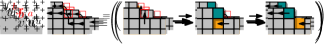
(b) Resolving non-consecutive instances of collision type (iv).

Figure 16: Three chain moves can locally replace a chain that induces a collision of type (iv).

With two chain moves, we can thus split the original chain into two independent chains. Parallel application of this idea to pairs of consecutive collisions in the same chain resolves any such occurrence in constantly many steps.

For all remaining (non-consecutive) collisions in each chain, we can apply a simplified version of the same mechanism in parallel, again splitting the chain at each instance of the collision. We illustrate the necessary preprocessing steps in Figure 16(b).

Since both variants of the schedule illustrated in Figure 16 use strictly local connectivity guarantees and the same cells that would have been used by the original chain, it is evident that the substitutions result in three legal transformations.

Appendix B Missing details of Section 3

See 3.1

Proof B.1.

We reduce from Planar Monotone 3Sat. For each instance $\varphi$ of Planar Monotone 3Sat, we start by constructing a Parallel Sliding Squares instance $\mathcal{I}_{\varphi}$ by means of the previously outlined gadgets. We now show that $\varphi$ has a satisfying assignment $\alpha(\varphi)$ if and only if there exists a schedule of makespan $1$ that solves $\mathcal{I}_{\varphi}$.

Claim 2.

If $\varphi$ has a satisfying assignment $\alpha(\varphi)$, there is a schedule of makespan $1$ for $\mathcal{I}_{\varphi}$.

Consider the satisfying assignment $\alpha(\varphi)$ for $\varphi$, and let $\alpha(x_{i})$ refer to the Boolean value assigned to $x_{i}$, i.e., true or false. We argue based on $\alpha(\varphi)$, as follows.

For each $x_{i}$, we demonstrate a feasible parallel chain move based on $\alpha(x_{i})$ that can fill the target cell. In case that $\alpha(x_{i})=\texttt{true}$, we displace robots along the “negative” side of the gadget, breaking connectedness with incident negative clauses during the transformation, as depicted in Figure 5(b). During this transformation, the remaining squares within the gadget form a connected shape with each of the incident positive clause gadgets. By mirroring this pattern vertically, we can define an analogous chain move for the negative case. Clearly, these transformations are collision-free and the variable gadgets have a joint, connected backbone.

It remains to argue that all clause gadgets retain a connection to this backbone, i.e., that there exists a single connected backbone. This is the case if and only if each clause gadget is incident to a variable gadget with a matching Boolean value assignment. Choosing our parallel transformations based on $\alpha(\varphi)$ therefore yields a schedule of makespan $1$ for $\mathcal{I}_{\varphi}$.

Claim 3.

If there is a schedule of makespan $1$ for $\mathcal{I}_{\varphi}$, then $\varphi$ has a satisfying assignment.

In any feasible schedule of makespan $1$, all cells that are occupied in both configurations of $\mathcal{I}_{\varphi}$ either retain the same square, or, if the square leaves, are occupied by another square in the same transformation. A feasible schedule can thus only consist of chain moves that connect the two differing positions in the variable gadgets, and potentially some number of circular chain moves. As the latter neither assist in preserving connectivity, nor in obtaining the target configuration, we assume without loss of generality that no such circular chain exists.

Recall that the configurations only differ in $2m$ cells, where $m$ is the number of variables in $\varphi$. It directly follows that the chain moves are limited to a single variable gadget each: As highlighted in Figure 17(a), the squares that connect variables to one another and to clauses cannot be moved as a result of the connected backbone property.

(a) The hatched portions cannot be moved without violating the backbone property.

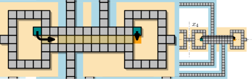
(b) Further arguments show that the construction holds even if collision type (iv) is ignored.

Figure 17: Feasible schedules perform one chain move within each variable gadget.

It remains to show that a feasible schedule of makespan $1$ for $\mathcal{I}_{\varphi}$ always implies a satisfying assignment for $\varphi$. To do this, we show that each chain move disconnects either all incident positive or negative clauses from a variable gadget. We start with the excess square in the left circle of the variable gadget, which can reach exactly two cells that are occupied in the target configuration, either diagonally above or below. From this point onward, due to the various collision restrictions, the chain can only push towards the right circle in a straight line, disconnecting the assignment strip from adjacent prongs during its transformation. With further arguments, our construction remains functional even if collision type (iv) may occur in legal transformations: No inclusion of convex transitions in the chain allows for structurally different schedules, as briefly outlined in Figure 17(b).

We conclude that a schedule of makespan $1$ consists of one chain move per variable gadget, and that these moves cause either all positive or negative clause prongs to lose connection to the variable during the transformation. Assigning each variable a Boolean value based on the direction taken by the excess square in its variable gadget therefore yields a satisfying assignment for $\varphi$. Claims 2 and 3 conclude the proof.

See 3.3

Proof B.2.

To prove this, it suffices to show that any instance $\mathcal{I}_{\varphi}$ created by our hardness reduction can be solved in $2$ parallel transformations without solving the underlying satisfiability question. Recall that the two configurations in $\mathcal{I}_{\varphi}$ differ only in positions within the variable gadgets. We show two parallel steps that solve a variable gadget while moving only the emphasized modules in Figure 18. Note that, since only the yellow modules are moved, this preserves connectivity throughout the process.

Figure 18: Two transformations solve a variable gadget without satisfying the Planar Monotone 3Sat instance.

Appendix C Missing details of Section 4

In this section, we give the omitted details for the algorithm given in Section 4.

C.1 Skeleton algorithm (Section 4.1)

We now give the details on the construction of the skeleton. Given a collection of modules $M$. Let $M[i]$ be the subset of $M$ of modules with $x$ coordinate $i$, likewise let $M[i,j]$, where $j>i$, be the set of all modules with $x$ coordinate in the interval $[i,j]$. We can compute a skeleton $S$ of a configuration as follows in Algorithm 1.

Algorithm 1 Given a configuration $C$, compute a skeleton $S$ of $C$.

  $i\leftarrow 0$

  $S\leftarrow\{\emptyset\}$

  $V\leftarrow\{\emptyset\}$

  while $C[i]\neq\{\emptyset\}$ do

     Add each maximally connected component of $C[i]$ to $V$

     $i\leftarrow i+2$

  end while

  $V\leftarrow V\cup\{C\setminus V\text{ and }V\text{'s 1-neighborhood}\}$

  $S\leftarrow V$

  $i\leftarrow 0$

  while  $V[i]\neq\{\emptyset\}$ do

     Create a graph $G$ with a vertex for each component in $V[i,i+2]$.

     for Each pair of vertices $v_{1},v_{2}\in G$ do

        if  $v_{1}$ $v_{2}$ are connected by a path in $C[i]\cup C[i+1]\cup C[i+2]$ containing no other element of $V[i,i+1,i+2]$ then

           Add an edge $\{v_{1},v_{2}\}$ to $G$ with a weight equal to the number of modules in the shortest such path.

        end if

     end for

     Compute a minimum spanning forest $F$ of $G$

     For each edge in $E(F)$ add the corresponding modules of $C$ to $S$.

     while $S$ has a cycle $L$ of length greater than $4$ do

        Use Lemma C.1 to break $L$

     end while

     $i\leftarrow i+2$

  end while

  while $S$ has $4$-cylces that are not disjoint do

     Apply Lemma C.3 to remove one of the cycles.

  end while

  return  $S$

Lemma C.1.

If the dual graph $G$ of a skeleton $S$, has a cycle $L$ of length of 4. $S$ can be modified so that it is still a skeleton and $L$ is broken.

Proof C.2.

First, note if $G$ has a 4-cycle $f$ and at least 2 modules of this cycle are also elements of $L$, then one element of $f$ can be removed from $S$. At least two modules of $f$, $a,b$ are connected by $L$. We may be able to remove one of them from $S$ breaking $L$. However if $a$ or $b$ have a neighboring module that is an element of $S$ but not of $f$ or $L$, they might not be removable without disconnecting $S$. However, if $a$ and $b$ have this many neighbors one of the other two modules of $f$ is safe to remove. As any of their potential neighbors are either elements of $f$ or adjacent to a neighbor of $a$ or $b$.

Therefore we assume for any two east-west adjacent modules of $L$, they do not both simultaneously have a south neighbor that is an element of $S$, or likewise, they both do not have north neighbors that are elements of $S$. As the existence of these simultaneous neighbors would form a $4$-cycle. We now prove there is always a module that can be removed from $L$, by considering narrower and narrower cases.

Suppose there is a module $r\in L$ that has a north neighbor $r_{n}$ that is not an element of $S$. Then, by the construction of $S$ in Algorithm 1, either $r_{n}$ has a west or east neighbor that is an element of $S$ and hence was not added to $V$ initially. Or $r_{n}$ was an element of $S$ but was later removed from $S$ to break a cycle. However, we will maintain the invariant that when we remove a module from $S$ to break a cycle it always has a north, east, or west neighbor that is an element of $S$. Therefore if $r$ is removed from $S$, $r_{n}$ will still be adjacent to an element of $S$ through a north, east, or west neighbor. Hence, if there is a module $r\in L$ such that $r$ has no south neighbor, and if it has a north neighbor $r_{n}$, $r_{n}$ is not an element of $S$, we can remove $r$ from $S$, breaking $L$.

Suppose every module of $L$ has a north or south neighbor. Observe, that this is possible as shown in Figure 19. As $L$ is a cycle in a geometric grid graph, there must be a sequence of three modules $a,b,c\in L$ that form a “corner”, an L-shaped arrangement where $a$ and $b$ are north/south neighbors and $b,c$ are east/west neighbors. Assume $b$ is the north neighbor of $a$ and the east neighbor of $c$. That is, $a,b,c$ form a “top-left” corner of $L$, with $b$ in the middle. If $b$ has no neighbors other than $a$ and $c$, then we can remove it from $C$.

Therefore suppose $b$ has a north neighbor $b_{n}$. If $b_{n}\in S$, then the only neighbor of $c$ that can be an element of $S$ is its east neighbor, as otherwise a 4-cycle would be formed by $b_{n},b,c,c_{n}$ or $b,c,c_{s},a$ (where $c_{n}$ and $c_{s}$ are $c$’s north and south neighbors, respectively). Therefore, if $b_{n}\in S$, we can remove $c$ from $L$ as its east neighbor must be an element of $L$, and if it does have north or south neighbors, they are adjacent to $b_{n}$ or $a$. Similarly if $b$ has a west neighbor, $b_{w}$, which is an element of $S$, $a$ can be removed from $S$. By the arguments made at the start of this proof, if $b_{n}\notin S$ then $b_{n}$ has a west or east neighbor that is an element of $S$. So if $b$ is removed from $S$, $b_{n}$ will still be adjacent to a module of $S$. As a consequence if $b$ has no west neighbor $b_{w}$ and $b_{n}\notin S$ we can remove $b$ from $S$.

Finally, consider the case that $b$ has a west neighbor $b_{w}$. As argued earlier, if $b_{w}\in S$ then $a$ can be removed from $S$. So suppose $b$ has a west neighbor $b_{w}\notin S$. We now have two cases:

$b_{w}$ has a neighbor $x\neq b$, where $x\in S$

We can remove $b$ from $S$.

$a$ has a west neighbor $a_{w}$:

If $a_{w}\in S$, then $b$ can be removed from $S$ as $b_{w}$ is adjacent to $a_{w}$. If $a_{w}\notin S$ but has a west neighbor that is an element of $S$, we can add $a_{w}$ to $S$ and remove $a$ and $b$ from $S$. We remove $a$ and $b$ instead of just $b$ in case adding $a_{w}$ forms a new cycle with its west neighbor and $a$. If $a_{w}$ does not have a west neighbor that is an element of $S$ then we can add $a_{w}$ to $s$ and remove $b$ from $S$.

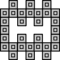
Figure 19: A large cycle where every module has a north/south neighbor in $S$.

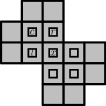
Figure 20: Two intersecting $4$-cycles. The top left cycle, labeled as in the proof of Lemma C.3.

Lemma C.3.

If the dual graph of a skeleton $S$ has two intersecting $4$-cycles then one of the cycles can be broken.

Proof C.4.

Let $c_{1}$ and $c_{2}$ be two $4$-cycles of the dual graph of $S$ such that $c_{1}\cap c_{2}\neq\{\emptyset\}$. We assume intersection of $c_{1}$ and $c_{2}$ is exactly one module $x$. It is trivial that in a grid graph, the intersection of two distinct $4$ cycles can only be 1 or 2 elements or else $c_{1}$ and $c_{2}$ are the same cycle. If the intersection of $c_{1}$ and $c_{2}$ is precisely two elements, then $c_{1}\cup c_{2}$ would form a cycle of length $6$, in this case we could apply Lemma C.1.

Without loss of generality assume that the shared module, $x$, is the bottom right module of $c_{1}$ and the top left module of $c_{2}$. Let $\chi$ represent the union of these two cycles, $\{c_{1}\cup c_{2}\}$.

First, we handle a “base case”. Suppose for every module $m\in C$ the only neighbors of $m$ that are elements of $S$ are also elements of $\chi$. Note, that this implies that the entirety of the skeleton is $\chi$ as if there were some module of $S$ that is not part of these cycles, by assumption, it is not adjacent to any module of $\chi$, and $S$ would be disconnected. In this case, if there is a module of $\chi$ other than $x$ with no neighbor outside of $S$, we can remove it from $S$ and break one of the cycles. Otherwise every module besides $x$ has a neighbor not in $S$, an example of one such configuration is shown in Figure 20. In this case, any module of $\chi$ can be removed from $S$ and be replaced with a vertex adjacent module not in $S$.

Now, we assume some module of $\chi$ has a neighbor $y$ where $y\in S$ but $y\notin\chi$. Label the top right module of $c_{1}$ $r$, the bottom left $l$ and the top left module $m$. Without loss of generality assume $y$ is adjacent to some module of $c_{1}$, some short casework follows.

Suppose $y$ is adjacent to $m$. If $r$ has a north neighbor it must be the east neighbor of $y$, and if $r$ has an east neighbor, it is adjacent to an element of $c_{2}$, by our assumed arrangement. Therefore we can remove $r$ from $S$.

Suppose there is no module of $S$ adjacent to $m$. If $y$ is adjacent to $r$ then we then try to remove $m$ from $S$. $m$ can have two neighbors outside of $c_{1}$. A north neighbor and a west neighbor $c_{w}$. $m$ having more neighbors only makes removing $m$ while maintaining skeleton properties harder, so assume $m$ has both neighbors. $y$ must be the north neighbor of $r$, otherwise it would form at least a 6 cycle with $c_{2}$. Therefore $c_{n}$ is adjacent to $y$. So of $m$ neighbors, removing $m$ from $S$ could only leave $c_{w}$ unadjacent to $S$. If $l$ has a west neighbor $l_{w}$ and $l_{w}\in S$, then we can safely remove $m$ from $S$. If $l_{w}\notin S$, then we can add $l_{w}$ to $S$ and remove $m$. It may be possible that adding $l_{w}$ to $S$ creates a large cycle in $S$. However, this cycle would necessarily use $x$ and one other module of $c_{2}$, and as argued in the proof of Lemma C.1 if a large cycle involves at least two modules of a 4-cycle, that 4-cycle can be broken. So, we add $l_{w}$ and remove $m$, and if a large cycle is formed, we remove a module of $c_{2}$ from $S$.

If $l$ has no west neighbor then then we remove $l$ instead of $m$. If $l$ has a south neighbor, that module must be adjacent to a module of $c_{2}$ and is therefore adjacent to another module of $S$, other than $l$.

Lemma C.5.

The subconfiguration $S$ created by Algorithm 1 is a skeleton of $C$.

Proof C.6.

There are three things we need to prove about $S$. One, it is a valid subconfiguration of $C$. Two, every module of $C$ is an element of $S$ or adjacent to $S$. Three, $S$ has no cycle larger than a $4$-cycle, and all $4$-cycles are disjoint.

$S$ is a valid subconfiguration of $C$:

First, ignore the modifications made to $S$ in the while loop on line 20. We construct $S$ by taking three sequential subsets of $V$, $V[i]$, $V[i+1]$, and $V[i+2]$ and connecting them via a spanning forest. We then connect $V[i+2]$, $V[i+3]$, and $V[i+4]$. Due to the overlap of these $V$’s by the end of our iteration we have connected every element of $V$, as long as $C$ is a connected configuration. So $S$ is a connected configuration. The modifications on line 20 cannot disconnect $S$, as they take a cycle $L$ of $S$, and remove exactly one element of $L$ from $S$.

Every element of $C$ is an element of $S$ or adjacent to an element of $S$:

By our formulation of $V$, initially every element of $C$ is either an element of $V$ or adjacent to $V$. So by initializing $S$ to $V$, $S$ immediately meets this condition. Hence, the only way to break this condition is in the while loop on line 20 where modules are removed from $S$. However, by Lemma C.1 these modifications maintain the desired adjacencies.

$S$ has no cycle larger than a $4$-cycle and all $4$-cycles are disjoint:

We remark that it may be impossible to remove all $4$-cycles. For example, near the top of Figure 21 there is an example of a $4$-cycle must be included in $S$ or else some module of $C$ will not be adjacent to $S$. The fact that there are no large cycles in $S$ and all $4$-cycles are disjoint follows from Lemmas C.1 and C.3. Algorithm 1 uses these lemmas inside while loops to remove any unwanted cycles until no more exist.

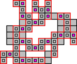
Figure 21: The skeleton of a configuration, outlined in red. Modules with grey squares are modules added to the skeleton from the initial segments, modules with purple squares are ones added to the skeleton in steps 4 and 8 of Algorithm 1

Figure 22: A large cycle can be created when connecting $V[i]$ to $V[i+1]$ (modules added to $S$ in red).

C.2 Omitted details of Phase (I) (Section 4.1)

See 4.3

Proof C.7.

Let $r$ be the root of $S$. We can assume that $r$ is initially a leaf of $S$, so that when we recurse on subtrees the maximum number of children of a node is 3. By induction on $n$.

Base case: When $1/3n\leq w$, $S_{r}$ satisfies the requirements of the lemma.

Inductive step: If a child $c$ of $r$ satisfies the requirements, we are done. If $|S_{c}^{*}|<w$ for every child $c$ of $r$, then $|S_{r}^{*}|\leq 3w-2$ since the maximum number of children is 3, thus we are in the base case. Else, $|S_{c}^{*}|>3w$ for some child $c$ of $r$ and, by inductive hypothesis, the claim is true for a subskeleton of $S_{c}$.

See 4.4

Proof C.8.

We show this by induction. The base case is when the conditions are already true. We update $S_{c}$ by reassigning the modules $S_{c}^{*}$ contained in other exoskeletons to their respective exoskeletons. If all modules in $M$ are in $N^{*}[c]$, we can delete $c$ from the skeleton, since all such modules can be supported by either $c$’s sibling (if it exists), $d$, or $d$’s parent. For the inductive step, we focus on the deepest node $c^{\prime}$ of $S_{c}$ that does not satisfy the conditions and let $d^{\prime}$ be its parent. We first assume that $S_{c^{\prime}}^{*}\subseteq N^{*}[{c^{\prime}}]$ and that $\deg(d^{\prime})=2$. If the neighborhoods of $c^{\prime}$ and $d^{\prime}$ do not contain nonlocal pieces of the skeleton or exoskeletons, then the modules in $N^{*}[c^{\prime}]\setminus N^{*}[d^{\prime}]$ can all freely move on the perimeter of $S_{c^{\prime}}$ (Figure 8(a)). We then move them to $N^{*}[d^{\prime}]$. Else, if the perimeter of $S_{c^{\prime}}$ is obstructed by nonlocal parts, we can move the skeleton modules of $S_{c^{\prime}}$ along the perimeter of the nonlocal parts. This will not break connectivity because we can temporarily “park” modules in $M$ in the perimeter of modules not in $M$. If $M$ is not a cut set, an empty position in $N^{*}[d^{\prime}]$ can easily be filled within 2 parallel moves. An interesting case occur when $M$ is a cut set module and we must move the parent $m$ of $d^{\prime}$ to fill an empty position (Figure 8(b)). In this situation, $m$ must have degree 3, or else $M$ is not a cut set, and $N^{*}[d^{\prime}]\cap N^{*}[c^{\prime}]$ must be full, or else we can fill in a position there more easily. Since $N^{*}[d^{\prime}]\cap N^{*}[c^{\prime}]$ is full and connected to a nonlocal part of the configuration, moving $m$ does not break connectivity. We can then move move the module in $d^{\prime}$ to $m$, restoring the connectivity with $m$’s parent. That creates an empty position in $N^{*}[d^{\prime}]\cap N^{*}[c^{\prime}]$ that can be filled using one of the previous techniques. So far we avoided moving any module in a nonlocal structure. That, however, might be unavoidable in the case that skeleton modules in $S_{c^{\prime}}$ are part of the shells of exoskeletons (Figure 8(c)). That is only possible if the core of an exoskeleton intersects $N^{*}[d^{\prime}]\cup N^{*}[c^{\prime}]$ at a degree-2 bend, by the skeleton definition. If this core cell is full, moving skeleton modules of $S_{c^{\prime}}$ do not affect connectivity of their exoskeletons. Else, such a cell is empty, but its neighborhood must be full by properties 3 and 4 of exoskeletons. We arrive at the same conclusion that moving skeleton modules of $S_{c^{\prime}}$ is safe. We now address the case when $\deg(d^{\prime})>2$ and $S_{c^{\prime}}^{*}\subseteq N^{*}[c^{\prime}]$ (Figure 8(d)). We just need to fill $N^{*}[d^{\prime}]\cap N^{*}[c^{\prime}]$. Using techniques from the previous cases, we can always find paths from a module in $N^{*}[c^{\prime}]\setminus N^{*}[d^{\prime}]$ to an empty position in $N^{*}[d^{\prime}]\cap N^{*}[c^{\prime}]$ while avoiding $d$ and its parent (which is either outside or in the boundary of $N^{*}[d^{\prime}]\cap N^{*}[c^{\prime}]$), and avoiding cells in shells of exoskeletons. For the same reasons as before, moving modules along such path does not break connectivity. Finally, we address the case when $S_{c^{\prime}}^{*}\not\subseteq N^{*}[c^{\prime}]$. By the choice of $c^{\prime}$ (deepest) the children of $c$ satisfy the conditions in the lemma, and $N^{*}[c^{\prime}]$ is not full. Then $c$ must have degree 2 and there is a single empty position in $N^{*}[c^{\prime}]$, i.e., $N^{*}[c^{\prime}]\setminus\{N^{*}[p]\cup N^{*}[q]\}$ where $p$ and $q$ are the children of $c$ (Figure 8(e)). Using the same arguments as above, we can find a path from a module outside $N^{*}[c^{\prime}]$ to this empty position as shown in the figure. That makes a solid $3\times 3$ square of modules centered at $c$. We can then make an exoskeleton with $c$ as its root.

See 4.6

Proof C.9.

In all cases of Inchworm-Push, local connectivity is not broken since the children of $d$ are full by property 4 ($N^{*}[d]$ remains connected after removing the moving modules). Thus, connectivity could only be broken for nonlocal parts of the configuration. This happens if the modules in $\pi$ are also part of nonlocal shells. Assume the orientation of Figure 9, i.e., $p$ is above $d$ and, in case (i) $c$ is below $d$, and in cases (ii–iii) $c$ is to the left of $d$. Note that if the shell of any nonlocal cell contains a moving module in cases in Figure 9(b) and (d), then cell $e$ depicted in the figure must not be empty, since it would also be in this cells shell. Thus, if we assume that a moving module is part of a nonlocal structure, we must be in case (i), or in case (ii) when $e$ is the cell to the northeast of $c$ (Figure 9(a) and (c)). We argue first for case (i). The nonlocal part of the exoskeleton must have a core cell in the southeast of $c$ or two cells to the east of $c$ (or both). Let $s$ and $q$ be such cells respectively. If the cell to the north of $q$ is also in the core of some exoskeleton, then $e$ is full since it’s a shell position, a contradiction. If either $s$ or $q$ are leaves then the moving modules are not part of a shell. Thus, assume the cell $t$ to the south of $q$ (and east of $s$) is a core cell. If all $s$, $q$ and $t$ are full, then connectivity is not broken. Note that only one of such cells can be empty by property 4. If either $s$ or $q$ are empty, then, by properties 3–4, all cells in $N^{*}(\{s,q\})$ are full. Then, connectivity is not broken as shown in Figures 11(a) and 11(b). If $t$ is the only empty cell in $N^{*}(\{s,q,t\})$, then the same argument holds as shown in Figure 11(c). The only other cell that could be empty is the cell $u$ to the southeast of $t$ if it is part of the core of an exoskeleton that is not local to $t$. By properties 3–4, $N(\{t,u\})$ is full, and connectivity is not broken (Figure 11(d)). Finally, all the arguments above can be repeated for case (ii) if we replace $c$ with $d$.

See 4.7

Proof C.10.

It is clear by its definition that Inchworm-Pull executes $\mathcal{O}(1)$ parallel moves. We focus first on the connectivity of stage 1. Let $p_{i}$ and $q_{i}$ be one of the empty positions and its chosen child, respectively, and let $M$ be the set of all such $p_{i}$ and $q_{i}$. Similar to Inchworm-Push, when the neighborhood of $\{p_{i},q_{i}\}$ does not intersect with nonlocal parts of the configuration, it is straightforward to check that the move from $q_{i}$ to $p_{i}$ does not break connectivity. That is $N^{*}(\{p_{i},q_{i}\})$ is connected by Properties 3–4 unless it contains at least two nonlocal empty core cells. In such cases, both $p_{i}$ and $q_{i}$ are in the shell of a nonlocal part of an exoskeleton, which can only happen if $p_{i}$ and $q_{i}$ are degree-2 bends vertex-adjacent to another nonlocal degree-2 bend of an exoskeleton core (see the left purple module and its north-adjacent empty cell in Figure 11(e)). Let $p_{i}^{\prime}$ or $q_{i}^{\prime}$ be the empty cells vertex-adjacent to $p_{i}$ and $q_{i}$. If $p_{i}^{\prime}$ is empty and not in $M$, by Properties 3–4 $N^{*}(p_{i}^{\prime})\setminus\{p_{i}\}$ is connected and thus $N^{*}(\{p_{i},q_{i},p_{i}^{\prime}\})$ is connected (as in Figure 11(e)). The same is true for $q_{i}^{\prime}$. Else, both $p_{i}^{\prime}$ or $q_{i}^{\prime}$ are in $M$, i.e., part of the same parallel move. Note that $p_{i}$ and $q_{i}$ induce a domino. The dominoes induced by all cells in $M$ can be adjacent to at most two other dominoes (the worst case happening if $p_{i}^{\prime}$ or $q_{i}^{\prime}$ are in $M$). The maximal set of dominoes that share a vertex form a path. At the two endpoints of such a path, either $N^{*}(\{p_{i},q_{i}\})$ is connected, or $N^{*}(\{p_{i},q_{i},p_{i}^{\prime}\})$ as the cases above. Thus, the configuration contains a cycle around each domino path induced by $M$ and stage 1 does not break connectivity.

We now focus on stages 2–5 that move leaves of the exoskeleton. We again define $p_{i}$ as an empty core position, $q_{i}$ a leaf, and $M$ the set of $p_{i}$ and $q_{i}$ in the same stage. Again, these positions induce dominoes since $(p_{i},q_{i})\in M$ cannot be adjacent to another $(p_{j},q_{j})\in M$ by Property 4. If two dominoes $(p_{i},q_{i})$ and $(p_{j},q_{j})$ are vertex-adjacent, then $1\leq|x(q_{i})-x(q_{j})|\leq 3$, and at least one of them is not in $M$. In particular, the parallel movement depicted in Figure 11(f) would not happen, and one of the leaves would stay put. So either $N^{*}(\{p_{i},q_{i}\})$ is connected, or $p_{i}$ is vertex-adjacent to an empty position $p_{i}^{\prime}$ not in $M$. Then, $N^{*}(\{p_{i},q_{i},p_{i}^{\prime}\})$ is connected as in stage 1.

C.3 Omitted details of Phase (II) (Section 4.2)

We achieve Step 1 by applying Inchworm-Pull in $X_{h}$ until all empty core cells are gone, which is up to the height of $X_{h}$ many times, hence $\mathcal{O}(P)$ parallel moves.

We now describe Step 2. The main technical difficulty is that the path will intersect nonlocal parts of the configuration. Those will not be part of $X_{h}$ by the choice of $c$. We will use the connectivity properties of exoskeletons to “go through” the obstacles without breaking connectivity. Let $d$ be $c$’s east neighbor. From now on, we consider the exoskeleton rooted at $c$, $X_{c}$, and note that $h$ becomes one of the leaves of $\overline{X_{c}}$. We also make sure that, throughout the reconfiguration, $\overline{X_{c}}$ always contains $h$ as a leaf so that its connectivity is maintained with the parts of the original skeleton $S$ that were not converted into the exoskeleton $X_{c}$. To accomplish that, whenever we apply Inchworm-Pull to $X_{c}$, we choose, if possible, a child $q$ of an empty position $p$ that is not an ancestor of $h$.

Our immediate goal is to fill the three positions to the right (NE, E and SE) of $d$. If all are full, we move the labels $c$ and $d$ to the right. Else, we first try moving $d$ to the right using Inchworm-Push case (ii) if $d$ is not a cut vertex (Figure 12(a)). Else, the position to the E of $d$ is full and we verify if applying Inchworm-Push case (i) would break connectivity. If not we perform it. The remaining case is when, without loss of generality, we wish to fill the NE cell from $d$ and module $p$, to either the N or NW of $d$, is a cut vertex (Figure 12(b)). Then, we first fill the cells $(0,2)+c$ and $(-1,2)+c$ (shown in red in Figure 12(b)). We do so first for $(0,2)+c$, if it is empty, by moving up the two modules below it. That makes $c$ empty. We can then apply Inchworm-Pull four times to $X_{c}$, making it an exoskeleton again. Repeat the same for $(-1,2)+c$. Now, $p$ is no longer a cut vertex and we can apply Inchworm-Push case (i). After that, $c$ is again empty. Instead of using Inchworm-Pull, we can route the modules at $(0,2)+c$ and $(-1,2)+c$ that were recently filled, to $c$ and the empty position at distance 4 away from $c$ in $\overline{X_{c}}$ created by the four executions of Inchworm-Pull (Figures 12(d), LABEL: and 12(e)). This makes $X_{c}$ an exoskeleton again.

Eventually, $c$ moves 2 positions to the right of the bounding box, and $X_{c}$ has a $3\times 3$ square of full cells outside the bounding box. Step 3 is very similar to Step 2. First relabel the module above $c$ as $d$ and propagate the path upwards in the same way (Figure 12(f)), except that $d$ will never be a cut vertex and we can always use Inchworm-Push case (ii). Once the top edge is reached, relabel $c$ and $d$ accordingly to propagate the path downwards (Figure 12(g)). Note that after the relabeling, $X_{c}$ is an exoskeleton except for the “4-arity” of the empty core cells. That can be fixed with $\mathcal{O}(1)$ applications of Inchworm-Pull.

Lemma C.11.

The Scaffolding phase takes $\mathcal{O}(P)$ transformations and does not break connectivity.

Proof C.12.

The “T-shaped” structure created in this phase has size $\mathcal{O}(P)$ and, thus, require $\mathcal{O}(P)$ applications of Inchworm-Push and Inchworm-Pull. When applying Inchworm-Push case (i), the extra moves guarantee that connectivity is not broken locally. At any moment, every component of $C\setminus X_{c}$ is either connected to the neighborhood of $h$, or to the shell of $X_{c}$. Whenever a path of $X_{c}$ shrinks due to an application of Inchworm-Pull we leave the cells in nonlocal parts of the original skeleton, so components of $C\setminus X_{c}$ potentially merge, but still are either connected to the neighborhood of $h$, or to the shell of $X_{c}$.

C.4 Omitted details of Phase (III) (Section 4.3)

After the scaffolding phase, we transform the exoskeleton of the scaffold into a sweep line at the west boundary of $B$, as illustrated in Figure 23. We then repeatedly clean and advance the sweep line until it reaches the east boundary of $B$, recall Figure 14.

(a)

(b)

(c)

Figure 23: We identify (a) a vertical portion of the skeleton that can be (b) transformed into a sweep line and (c) cleaned, simulatenously becoming a separator.

See 1 Consider the scaffold exoskeleton $X_{c}$ as defined in Section 4.2, and let $v_{1}\in\overline{X_{c}}$ refer to its $xy$-minimal core cell. Due to Lemma C.11, $C$ contains a subskeleton $X_{\ell}$ that contains the modules between the right edge of the bounding box $B$ and the right edge of the extended bounding box $B^{\prime}$, such that the shell of $X_{\ell}$ is fully occupied. This means that the modules in $C\cap\overline{X_{\ell}}$ are free.

Let $B_{y}$ refer to the height of the minimal bounding box of $C$. Due to the $4$-arity of the depth of unoccupied cells in skeletons, at least $\nicefrac{{3}}{{4}}B_{y}-2$ cells in $\overline{X_{\ell}}$ contain a module. To obtain a sweep line, every core cell $v\in\overline{X_{\ell}}$ that has $y(v)\not\equiv 1(\bmod 3)$ must be occupied. This requires exactly $\nicefrac{{2}}{{3}}B_{y}-2$ modules, so a sequence of at most $B_{y}$ chain moves in $\overline{X_{\ell}}$ suffices to reconfigure $X_{\ell}$ into a sweep line of $C$. Clearly, this sweep line is a separator; due to the initial construction of $X_{c}$, its west half-space is empty.

See 4.11

Proof C.13.

Consider a sweep line ${\ell}$ in a configuration $C$ and let $M_{i}$ refer to an arbitrary solid meta-module in ${\ell}$ with center cell $v_{i}$. We show that $M_{i}$ can be cleaned in at most $2$ transformations, if neither of its neighbors in ${\ell}$ is being cleaned simultaneously. As a result, the following procedure can be used to clean all leading (resp., trailing) modules in parallel, resulting in a schedule of total makespan at most $4$.

Consider the $xy$-minimal empty cell $v_{\varnothing}\in\textsc{w}(M_{i})$ and denote the distance that separates it from $M_{i}$ by ${k=x(v_{i})-x(v_{\varnothing})-1}$. All cells in $\textsc{w}(M_{i})$ with $x$-coordinates larger than $x(v_{\varnothing})$ are thus full, inducing a rectangle $R$ of $k\times 3$ modules. Note that we can assume without loss of generality that such a cell $v_{\varnothing}$ exists, as $M_{i}$ does not affect whether ${\ell}$ is clean otherwise.

We differentiate based on the three $x$-maximal cells in $\textsc{w}(M_{i})\setminus R$, denoted by $\textsc{w}^{k}_{1},\textsc{w}^{k}_{2},\textsc{w}^{k}_{3}$ in south to north order, see Figure 24(a). Assume for now that $i\in[2,h-1]$, i.e., that $M_{i}$ has two neighbors in the sweep line ${\ell}$.

If $\textsc{w}^{k}_{2}\notin C$, the modules in $R$ that have the same $y$-coordinate as $v_{i}$ are free. We thus perform one of the two chain moves shown in Figure 24(a) from $v_{i}$ to either $\textsc{w}^{k}_{2}$ or $\textsc{w}^{k}_{3}$.

(a) Trivial cases: $\textsc{w}^{k}_{2}\notin C$.

(b) Not all adjacent cells north of $R$ are occupied, and $\textsc{w}^{k}_{2}\in C$.

(c) All adjacent cells north of $R$ are occupied, and ${\textsc{w}^{k}_{2}\in C}$.

Figure 24: “Cleaning” schedules that move only west or north. These are independent of $\textsc{w}_{3}$.

If $\textsc{w}^{k}_{2}\in C$, the same set of modules may not be free. In particular, this is true of the module immediately east of $\textsc{w}^{k}_{2}$. By definition, at least one of $\textsc{w}^{k}_{1}$ and $\textsc{w}^{k}_{3}$ is unoccupied. Assume without loss of generality that $\textsc{w}^{k}_{3}\notin C$. The following procedure can be mirrored vertically for the case that $\textsc{w}^{k}_{3}\in C$, as then $\textsc{w}^{k}_{1}\notin C$.

If there is at least one unoccupied cell adjacent immediately north of $R$, it follows that its neighbor module in $R$ is free. Let $v_{\textsc{n}}$ refer to the $x$-maximal empty cell that meets these criteria. We perform two chain moves, placing a module in $v_{\textsc{n}}$, see Figure 24(b). If there is no such empty cell $v_{\textsc{n}}$, we perform the two moves in Figure 24(c), occupying $\textsc{w}^{k}_{3}$.

It remains to argue that $M_{1}$ and $M_{h}$ can be cleaned in a similar manner. We argue for the northernmost meta-module $M_{h}$, but the same line of argumentation applies to $M_{1}$. If $\textsc{w}^{k}_{2}\notin C$, the schedules depicted in Figure 24(a) are immediately applicable. Otherwise, we do not fill positions north of $R$, but only south, otherwise proceeding in the same manner. In particular, the northernmost modules in $R$ are always free if $\textsc{w}^{k}_{3}\notin C$.

See 4.12

Proof C.14.

We define schedules that allow non-adjacent meta-modules to move westward in parallel and use these to shift all meta-modules west in two phases, as illustrated in Figure 14.

Let $M_{i}$ refer to an arbitrary meta-module in ${\ell}$ with an occupied center cell $v_{i}$. We show that $M_{i}$ can be translated to the west by one unit by a schedule of makespan at most $6$, if neither of its neighbors in ${\ell}$ is being moved simultaneously. The following procedures can thus be used to shift all leading (resp., trailing) modules in parallel. Note that the first claim only handles meta-modules which have two adjacent meta-modules in ${\ell}$. For the northernmost (resp., southernmost) meta-module in ${\ell}$, we give a separate case analysis.

Claim 4.

We can translate any meta-module $M_{i}$ with $i\in[2,h-1]$ to the west by one cell in at most $6$ transformations, without moving any module east.

We differentiate based on modules in the cells with $x$-coordinate exactly $x(v_{i})-2$, which we denoted by $\textsc{w}_{1},\textsc{w}_{2},\textsc{w}_{3}$ in south to north order. There exist eight possible configurations, which we identify by the power set of $\{\textsc{w}_{1},\textsc{w}_{2},\textsc{w}_{3}\}$ and group into six equivalence classes according to symmetry along the $x$-axis, see Figure 25. As we cannot be certain that modules in $\{\textsc{w}_{1},\textsc{w}_{2},\textsc{w}_{3}\}$ are free, we mark them with and avoid moving them.

Figure 25: There are $2^{3}=8$ possible configurations of the cells $\textsc{w}_{1},\textsc{w}_{2},\textsc{w}_{3}$, all shown here.

We start by identifying and handling two trivial cases. Firstly, if every cell west of $M_{i}$ is already occupied, i.e., $\textsc{w}(M_{i})\subseteq C$, we simply slide the module located immediately west of $v_{i}$ to the east by one unit, inducing a clean meta-module at $v_{i}^{\prime}=(x(v_{i})-1,y(v_{i}))$.

Secondly, if $C\cap\{\textsc{w}_{1},\textsc{w}_{2},\textsc{w}_{3}\}=\varnothing$, i.e., none of the west-adjacent cells are occupied, the schedule in Figure 26(a) can easily be verified: No collisions occur, and a connected backbone is maintained. While the illustrated schedule is applicable only if $M_{i}$ is leading, we can simply reverse and rotate the moves by $180^{\circ}$, in case $M_{i}$ is trailing.

(a) Leading, $\textsc{w}_{1}$, $\textsc{w}_{2}$, and $\textsc{w}_{3}$ are empty. This schedule can be rotated and reversed for trailing modules.

 

(b) Leading, $|C\cap\{\textsc{w}_{1},\textsc{w}_{2},\textsc{w}_{3}\}|=1$.

(c) Leading, $|C\cap\{\textsc{w}_{1},\textsc{w}_{2},\textsc{w}_{3}\}|=2$.

(d) Leading, $\{\textsc{w}_{1},\textsc{w}_{2},\textsc{w}_{3}\}\subset C$.

 

(e) Trailing, $|C\cap\{\textsc{w}_{1},\textsc{w}_{2},\textsc{w}_{3}\}|=1$.

(f) Trailing, $|C\cap\{\textsc{w}_{1},\textsc{w}_{2},\textsc{w}_{3}\}|=2$.

(g) Trailing, $\{\textsc{w}_{1},\textsc{w}_{2},\textsc{w}_{3}\}\subset C$.

Figure 26: Shifting meta-modules to the west. Schedules for the case that a meta-module has two neighbors: (a) visualizes the case in which the meta-module does not “collide” with other modules; leading meta-modules (b)–(d) and (e)–(g) trailing meta-modules, in case there are occupied cells directly to the west of the meta-module.

It remains to handle the case in which $C\cap\{\textsc{w}_{1},\textsc{w}_{2},\textsc{w}_{3}\}\neq\varnothing$ and at least one cell west of the meta-module in $\textsc{w}(M_{i})$ is unoccupied. We handle each case separately, using the schedules depicted in Figure 26. Based on whether $M_{i}$ is a leading or trailing meta-module, we refer to Figures 26(b) to 26(d) and Figures 26(e) to 26(g), respectively. Once again, due to their locality, the validity of these schedules can easily be verified: As neither $M_{i+1}$ nor $M_{i-1}$ move, a connected backbone will always be preserved, and no collisions can occur, meaning that we have successfully shifted $M_{i}$ to the west by one unit.

Claim 5.

We can translate any meta-module $M_{i}$ with $i\in\{1,h\}$ to the west by one cell in at most $6$ transformations, without moving any module east.

The arguments are similar to the proof of Claim 4. We refer to Figure 27 for an illustration of the local transformations based on occupied and free cells immediately adjacent to the respective meta-module. Furthermore, by mirroring this schedule along the $x$-axis, we further obtain a valid schedule for the southernmost meta-module, again for both the leading and trailing case.

(a) Leading, $\textsc{w}_{1}$, $\textsc{w}_{2}$, and $\textsc{w}_{3}$ are empty. This schedule can be rotated and reversed for trailing modules.

 

(b) Leading, $C_{\textsc{w}}\in\{\{\textsc{w}_{1}\},\{\textsc{w}_{3}\}\}$.

(c) Leading, $C_{\textsc{w}}=\{\textsc{w}_{1},\textsc{w}_{3}\}$.

(d) Leading, $C_{\textsc{w}}=\{\textsc{w}_{2}\}$.

(e) Leading, $C_{\textsc{w}}=\{\textsc{w}_{1},\textsc{w}_{2},\textsc{w}_{3}\}$.

(f) Leading, $C_{\textsc{w}}=\{\textsc{w}_{2},\textsc{w}_{3}\}$.

(g) Leading, $C_{\textsc{w}}=\{\textsc{w}_{1},\textsc{w}_{2}\}$.

 

(h) Trailing, $C_{\textsc{w}}\in\{\{\textsc{w}_{1}\},\{\textsc{w}_{3}\}\}$.

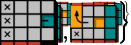
(i) Trailing, $C_{\textsc{w}}=\{\textsc{w}_{1},\textsc{w}_{3}\}$.

(j) Trailing, $C_{\textsc{w}}=\{\textsc{w}_{1},\textsc{w}_{2},,\textsc{w}_{3}\}$.

(k) Trailing, $C_{\textsc{w}}=\{\textsc{w}_{2}\}$.

(l) Trailing, $\C_{\textsc{w}}=\{\textsc{w}_{1},\textsc{w}_{2}\}$.

(m) Trailing, $C_{\textsc{w}}=\{\textsc{w}_{2},\textsc{w}_{3}\}$.

Figure 27: Shifting meta-modules to the west. Schedules for the case that a meta-module has only one neighbor: Let $C_{\textsc{w}}=C\cap\{\textsc{w}_{1},\textsc{w}_{2},\textsc{w}_{3}\}$. Subfigure (a) visualizes the case that $C_{\textsc{w}}=\varnothing$. Otherwise, leading meta-modules are handled in (b)–(g), and trailing in (h)–(m).

Due to their strictly local nature, all of our schedules for leading (resp., trailing) meta-modules can be performed in parallel. We first shift at all leading modules simultaneously, using the schedules outlined in Claims 4 and 5. This takes at most $6$ transformations. Afterward, we apply the same procedures to all trailing meta-modules in parallel, again taking at most $6$ transformations. We conclude that it is possible to obtain a sweep line ${\ell}^{\prime}$ with $x({\ell}^{\prime})=x({\ell})-1$ in at most $12$ transformations.

Upon completion, some meta-modules of the sweep line ${\ell}^{\prime}$ may be solid, and up to two squares per meta-module now additionally occupy the east half-space in a way that violates the separator property. We now show that ${\ell}^{\prime}$ can be made into a clean separator sweep line.

Consider any meta-module $M^{\prime}_{i}$ of ${\ell}^{\prime}$. If $\textsc{w}(M^{\prime}_{i})\subseteq C$, $M^{\prime}_{i}$ is clean by definition, see above. Otherwise, there exist at most two modules in $\textsc{e}(M^{\prime}_{i})$, immediately adjacent to the meta-module itself. Due to Lemma 4.11, $M^{\prime}_{i}$ can be cleaned in $2$ transformations; it only remains to argue that we can restore the separator conditions. With a simple chain move, we can place one of the two excess squares in $v^{\prime}_{i}$ and clean $M^{\prime}_{i}$ once more to free up $v^{\prime}_{i}$ again.

We clean each module at most three times, and all leading (resp., trailing) meta-modules in parallel, taking at most $3\cdot 4+2=14$ additional transformations. Afterward, we obtain a clean separator sweep line ${\ell}^{\prime}$ with $x({\ell}^{\prime})=x({\ell})-1$.

C.5 Omitted details of Phase (IV) (Section 4.4)

See 4.13

We start by making the sweep line ${\ell}$ in $C$ solid. To achieve this, we can simply apply the cleaning operation outlined in Lemma 4.11 in reverse. Even without parallelization, at least one meta-module of ${\ell}$ can be “un-cleaned” every $\mathcal{O}(1)$ transformations. There are $\mathcal{O}(P)$ many clean meta-modules, so we can obtain a solid sweep line in $\mathcal{O}(P)$ transformations.

To make $C$ into a $3$-scaled histogram, it remains to balance the modules in $C\setminus{\ell}$ such that for each $M_{i}\in{\ell}$, the number of modules in $C\cap\textsc{w}(M_{i})$ is a multiple of nine. Observe that there are at most $8$ “loose” modules in any horizontal strip induced by some meta-module $M_{i}$. We start with the strip induced by the topmost meta-module $M_{h}$. These modules can be iteratively moved to the strip induced by $M_{h-1}$ by $\mathcal{O}(1)$ transformations as depicted in Figure 28, and are thereby placed immediately adjacent to occupied cells within this strip. Now the number of modules in the strip of $M_{h}$ is a multiple of $9$, and there are at most $8$ loose modules in the strip of $M_{h-1}$.

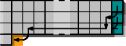
Figure 28: The depicted chain moves can be realized in $\mathcal{O}(1)$ transformations (and in reverse).

We repeat this procedure until we reach $M_{1}$, i.e., iteratively move loose modules down, and leave $3$-scaled strips behind.

Finally, after completion, there are at most $8$ loose modules located in the bottommost strip. These can trivially be moved immediately to the west of the solid sweep line by straight forward chain moves.

As the the bounding box has height $\mathcal{O}(P)$, this approach takes at most $\mathcal{O}(P)$ many transformations.

See 4.14

Proof C.15.

Assume without loss of generality that $C$ is $x$-monotone and that is base is located east. Let $R_{1},\ldots,R_{m}$ refer to the unique decomposition of $C$ into a minimal number of rectangles of width $3$, such that $R_{1}$ is the rectangle with $x$-maximal coordinates, see Figure 29. Note that by definition, $R_{1}$ spans the bounding box of $C$ from north to south. Such a decomposition can easily be computed in polynomial time, e.g., by a greedy algorithm. Our goal now is to move all rectangle strips $R_{i}$ to the south until they meet the boundary of $B$, or the boundary of another rectangle $R_{j}$, as illustrated in Figure 29.

   

Figure 29: Using a strip decomposition to make $C$ $xy$-monotone.

The schedule illustrated in Figure 30 can be performed in parallel by all rectangles that do not include a $y$-minimal cell in $B$. Note that, since this does not include $R_{1}$, the adjacent cells immediately east of each rectangle are occupied by modules of another rectangle. It follows that the modules we move are free during each transformation.

Figure 30: Inchworming a $3\times k$ ($k\geq 3$) rectangle to the south, in six transformations.

The parallel execution of these schedule moves all involved rectangles to the south by one unit. Afterward, we simply recompute the rectangle decomposition $R_{i}$ of $C$, and repeat. After at most $P$ repetitions, every rectangle contains a $y$-minimal cell in $B$. This implies that $C$ is an $xy$-monotone configuration.

Corollary C.16.

Any scaled, $xy$-monotone configuration can be translated by $k$ units in any cardinal direction, by at most $\mathcal{O}(k)$ strictly in-place transformations.

See 4.15

Proof C.17.

Note that by definition, the bounding boxes $B_{1}$ and $B_{2}$ share an $xy$-minimal corner. Without loss of generality, let this corner be anchored at $(0,0)$.

We assume that the base of $C_{1}$ (resp., $C_{2}$) lies south-west. If this were not initially the case, we could obtain such a configuration in makespan $\mathcal{O}(P_{1})$ (resp., $\mathcal{O}(P_{2})$) due to Lemma 4.14.

Let $v_{(i,j)}$ refer to the center cell $(3i+1,3j+1)$ of a meta-module $M_{(i,j)}$. Due to $xy$-monotonicity, if $v_{(a,b)}\in C_{1}$, then $v_{(c,d)}\in C_{1}$ for $c\leq a$ and $d\leq b$. This implies that we can use the “L”-shaped schedules as depicted in Figure 31 to move a meta-module along the slope of the configurations, taking $18$ moves regardless of distance. For any such set of paths that do not cross, this can be performed in parallel.

      

Figure 31: Moving modules through the interior of a $3$-scaled L-shape.

Our approach follows ideas by Fekete et al. [14, 17] to reconfigure histograms in a different model, which has also been explored experimentally for the sliding squares model [29]. For the remainder of this proof, we act as if $C_{1}$ and $C_{2}$ were not scaled and replace each meta-module with only its center cell $v_{(i,j)}$, placed now at exactly $(i,j)$. We describe a schedule that achieves our goal in terms of “L”-shaped paths as outlined above, which can be realized in parallel in the “real”, scaled configurations $C_{1}$ and $C_{2}$.

We use two diagonal lines with south-west slopes. Each line $L$ splits the extended bounding box into three disjoint sets $\textsc{n}(L)$, $\textsc{s}(L)$, and $L$. See Figure 32 for illustrations of the following definitions.

We define $L_{1}$ as the $xy$-maximal diagonal line such that $C_{2}\cap\textsc{s}(L)$ is a subset of $C_{1}\cap\textsc{s}(L)$. By definition, there exists at least one cell in $L_{1}$ that is occupied in $C_{2}$, but not in $C_{1}$. Further, let $L_{2}$ be the $xy$-maximal diagonal line that contains a module in $C_{1}$, but not in $C_{2}$.

Figure 32: We reconfigure according to $L_{1}$ (blue) and $L_{2}$ (red). Each square corresponds to a meta-module in the scaled configuration and moves occur according to Figure 31.

Using the methods outlined in [14] (Claim 4), we can compute a maximum matching between unoccupied cells in $L_{1}$ and excess occupied cells in $L_{2}$ such that there exist “L”-shaped paths between matched positions that do not cross. In any such maximum matching, either all unoccupied cells in $L_{1}$, or all occupied cells in $L_{2}$ are matched. We use the schedules from Figure 31 to move each corresponding meta-module in the scaled configuration to its matched center cell. As a result, either (a) every previously unoccupied cell in $L_{1}$ is now occupied, or (b) every excess module in $L_{2}$ has been removed. Updating both lines for the obtained configuration, it follows that either $L_{1}$ has moved north, or $L_{2}$ has moved south.

After at most $\max(P_{1},P_{2})$ iterations of this process, either $C_{1}\subset\textsc{n}(L_{2})$, or $C_{1}\subset\textsc{s}(L_{1})$. In either case, it follows that $C_{1}=C_{2}$.

As indicated in Section 4.4, we assumed that $n$ is a multiple of nine throughout the final phase. If this is not the case, we simply stack the excess modules in the column just east of the sweep line’s $x$-minimal module, starting at its $y$-minimal cell. This is briefly illustrated in Figure 15 and can be achieved with minimal modifications to Lemma 4.13. None of the subsequent transformations, i.e., those induced by Lemmas 4.14 and 4.15, ever move the $xy$-minimal module of the initial configurations, meaning that no adjustments must be made to the procedures to account for the excess modules.

Phase (IV) is compatible with instances of ${n\not\equiv 0(\text{mod }9)}$ modules.

C.6 Proof of the main theorem

See 4.2

Proof C.18.

Consider two configurations $C_{1},C_{2}$ contained in an $\nicefrac{{n}}{{2}}\times\nicefrac{{n}}{{2}}$ bounding box $B$. Define $C_{1}$ to contain the $n-1$ modules adjacent to the left and bottom edges of $B$ and a module at $(1,1)$. Define $C_{2}$ to contain the $n-1$ modules adjacent to the top and right edges of $B$ and a module at $(\nicefrac{{n}}{{2}}-1,\,\nicefrac{{n}}{{2}}-1)$. Then, the minimum bottleneck matching between full cells in $C_{1}$ and $C_{2}$ has bottleneck $\Omega(n)$, implying that a module must make $\Omega(n)$ moves. The makespan is then $\Omega(n)=\Omega(P)$, where $P$ is the perimeter of $B$.

See 4.1

Proof C.19.

Phases (I-IV) transform an arbitrary configuration into a scaled, $xy$-monotone histogram that has a south-west base within its extended bounding box $B^{\prime}$ in $\mathcal{O}(P)$ time. Due to Lemma 4.15, we can further reconfigure the resulting histogram into any other such histogram, using strictly in-place schedules of makespan at most $\mathcal{O}(P)$.

Given an instance $\mathcal{I}=(C_{1},C_{2})$, we simultaneously apply Phases (I-IV) to both configurations, obtaining two weakly in-place schedules that yield scaled, $xy$-monotone histogram configurations $H_{1},H_{2}$ with south-west bases and a shared $xy$-minimal module. We compute a feasible schedule $H_{1}\rightarrow^{*}H_{2}$ using Lemma 4.15 before and apply the previously computed schedule $C_{2}\rightarrow^{*}H_{2}$ in reverse. The result is a schedule $C_{1}\rightarrow^{*}C_{2}$ of makespan $\mathcal{O}(P)$.

Appendix D Computational complexity of the labeled variant

In this section, we consider the computational complexity of the labeled variant of our problem. In contrast to the unlabeled variant, the question whether there is a schedule with makespan $1$ transforming a given start into a given desired target configuration can be decided in polynomial time. However, the problem is still -complete from makespan $2$, and cannot be approximated within a factor less than $\nicefrac{{3}}{{2}}$.

Proposition D.1.

Let $\mathcal{I}$ be an instance of Labeled Parallel Sliding Squares. It can be decided in polynomial time whether there exists a schedule of makespan $1$ that solves $\mathcal{I}$.

Proof D.2.

We first check whether the respective start and target positions are in unit distance to one another. Otherwise, a schedule of makespan $1$ is not possible. Furthermore, we check whether every single transformation can be applied in parallel. To do so, we need two check whether (1) non of these cause collisions, and (2) if these transformation are connectivity-preserving. As only constantly many robots can cause collisions with any robot, we can check whether the proposed transformations are collision-free in $\mathcal{O}(n)$. For the second condition, we simply remove all robots that want to move from the configuration, and check whether the resulting graph is connected with some graph search algorithm. As our graph is sparse, this can be done in $\mathcal{O}(n)$.

Theorem D.3.

Let $\mathcal{I}$ be an instance of Labeled Parallel Sliding Squares. It is -complete to decide whether there exists a schedule of makespan $2$ that solves $\mathcal{I}$.

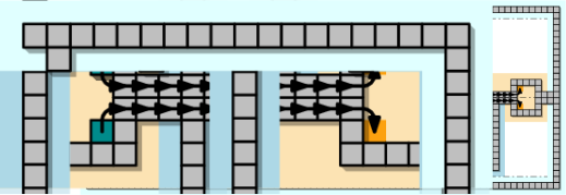
Figure 33: An overview of the hardness construction for the labeled variant of the problem.

Variable gadget.

The variable gadget for the labeled setting is similar to that of the unlabeled variant of the problem. It consists of two empty circles composed of $18$ squares each, one containing two additional squares in its interior, and the other containing two cells that need to be occupied in the target configuration, see Figure 34(a). These circles are connected by a solid, horizontal assignment strip of height $2$, to which individual clause gadgets are connected.

(a) Variable gadget and labeling.

(b) Clause gadget.

Figure 34: Illustrations of the variable gadget for the labeled problem variant.

Clause and backbone gadget.

Similar to the clause gadget of the unlabeled version, it consists of a thin horizontal strip that spans the gadgets of variables contained in the clause, and (up to) three vertical prongs that connect to the assignment strips of the incident variable gadgets. Apart from one square that needs to move one step to the right, the clause structure is identical in both configurations of the instance, as depicted in Figure 5(c). These additional squares are part of the backbone gadget that guarantees connectivity of the configuration during the second transformation step, as this does not necessarily satisfies the Boolean formula. To make this gadget work, we add some additional structure, above the topmost and below the bottommost clause that connects everything to the variables, as visualized in Figures 35, LABEL: and 33.

Figure 35: Backbone gadgets.

Proof D.4 (Proof of Theorem D.3).

The proof and construction is similar to the proof of Theorem 3.1, i.e., to the unlabeled variant. We again reduce from Planar Monotone 3Sat, i.e., we construct an instance $\mathcal{I}_{\varphi}$ of Labeled Parallel Sliding Squares from any given formula $\varphi$ by using the described gadgets. We show that $\varphi$ has a satisfying assignment $\alpha(\varphi)$ if and only if there exists a schedule of makespan $2$ that reconfigures $\mathcal{I}_{\varphi}$.

Claim 6.

If $\varphi$ has a satisfying assignment $\alpha(\varphi)$, there is a schedule of makespan $2$ for $\mathcal{I}_{\varphi}$.

Consider the satisfying assignment $\alpha(\varphi)$ for $\varphi$, and let $\alpha(x_{i})$ refer to the Boolean value assigned to $x_{i}$, i.e., true or false. We argue based on $\alpha(\varphi)$, as follows. Just as in the unlabeled variant, according to the assignment, we perform for every $x_{i}$ the respective chain move, as illustrated in Figure 34(a). In case that $\alpha(x_{i})=\texttt{true}$, this chain move breaks connectedness with incident negative clauses. Note that both chains of the assignment strip of a variable cannot move simultaneously. Furthermore, we also move all squares associated with the backbone in this very first move, as depicted in Figure 34(b). As $\alpha(\varphi)$ satisfies $\varphi$, this first parallel transformation maintains a connected configuration.

Afterward, we perform all other chain moves within the variable gadgets. As the connected backbone remains stationary during the second transformation, the whole configuration stays connected. Thus, the desired target configuration is reached after two parallel moves.

Claim 7.

If there is a schedule of makespan $2$ for $\mathcal{I}_{\varphi}$, then $\varphi$ has a satisfying assignment.

In any schedule of makespan $2$, not both horizontal chains of an assignment strip can move simultaneously, as this would require illegal transformations. However, in each of the two transformation steps, exactly one of the chains has to move. As we require a connected backbone during any transformation, we use this movement to the respective values to the associated variables. This assignment satisfies the given formula, as the configuration stays connected. Similar to the unlabeled variant, there are no other feasible moves within variables gadgets to guarantee both connectedness, and the desired makespan.

Depending on whether the negated assignment also fulfills the given formula, the backbone squares must move in the first transformation step as well, or not. Regardless of these movements, the configuration remains connected during the second transformation, as the schedule was legal by assumption. Claims 6 and 7 conclude the proof.

Corollary D.5.

The Labeled Parallel Sliding Squares problem is -hard: Unless $\P=\NP$, there is no polynomial-time $(1+\delta)$-approximation algorithm for $\delta\in[0,\nicefrac{{3}}{{2}})$.

Proof D.6.

To prove this, it suffices to show that any instance $\mathcal{I}_{\varphi}$ created by our hardness reduction can be solved in $3$ parallel transformations without solving the underlying satisfiability question. A connected backbone can be guaranteed by only moving all the squares corresponding to the backbone gadgets in parallel. Afterward, moving the squares within the variable gadgets (starting with the ones corresponding to setting the variable to true) are legal transformations, as the backbone property is maintained. Thus, after three steps, the target configuration is reached.

References

- [1] Zachary Abel, Hugo A. Akitaya, Scott Duke Kominers, Matias Korman, and Frederick Stock. A universal in-place reconfiguration algorithm for sliding cube-shaped robots in a quadratic number of moves. In Symposium on Computational Geometry (SoCG), pages 1:1–1:14, 2024. doi:10.4230/LIPIcs.SoCG.2024.1.
- [2] Hugo A. Akitaya, Esther M. Arkin, Mirela Damian, Erik D. Demaine, Vida Dujmovic, Robin Y. Flatland, Matias Korman, Belén Palop, Irene Parada, André van Renssen, and Vera Sacristán. Universal reconfiguration of facet-connected modular robots by pivots: The musketeers. Algorithmica, 83(5):1316–1351, 2021. doi:10.1007/s00453-020-00784-6.
- [3] Hugo A. Akitaya, Erik D. Demaine, Andrei Gonczi, Dylan H. Hendrickson, Adam Hesterberg, Matias Korman, Oliver Korten, Jayson Lynch, Irene Parada, and Vera Sacristán. Characterizing universal reconfigurability of modular pivoting robots. In Symposium on Computational Geometry (SoCG), pages 10:1–10:20, 2021. doi:10.4230/LIPIcs.SoCG.2021.10.
- [4] Hugo A. Akitaya, Erik D. Demaine, Matias Korman, Irina Kostitsyna, Irene Parada, Willem Sonke, Bettina Speckmann, Ryuhei Uehara, and Jules Wulms. Compacting squares: Input-sensitive in-place reconfiguration of sliding squares. In Scandinavian Symposium and Workshops on Algorithm Theory (SWAT), pages 4:1–4:19, 2022. doi:10.4230/LIPIcs.SWAT.2022.4.
- [5] Greg Aloupis, Sébastien Collette, Mirela Damian, Erik D. Demaine, Robin Flatland, Stefan Langerman, Joseph O’Rourke, Suneeta Ramaswami, Vera Sacristán, and Stefanie Wuhrer. Linear reconfiguration of cube-style modular robots. Computational Geometry, 42(6-7):652–663, 2009. doi:10.1016/J.COMGEO.2008.11.003.
- [6] Aaron T. Becker, Sándor P. Fekete, Phillip Keldenich, Matthias Konitzny, Lillian Lin, and Christian Scheffer. Coordinated motion planning: The video. In Symposium on Computational Geometry (SoCG), pages 74:1–74:6, 2018. doi:10.4230/LIPICS.SOCG.2018.74.
- [7] Julien Bourgeois, Sándor P. Fekete, Ramin Kosfeld, Peter Kramer, Benoît Piranda, Christian Rieck, and Christian Scheffer. Space ants: Episode II - Coordinating connected catoms. In Symposium on Computational Geometry (SoCG), pages 65:1–65:6, 2022. doi:10.4230/LIPIcs.SoCG.2022.65.
- [8] Zack Butler and Daniela Rus. Distributed planning and control for modular robots with unit-compressible modules. The International Journal of Robotics Research, 22(9):699–715, 2003. doi:10.1177/02783649030229002.
- [9] Matthew Connor, Othon Michail, and George Skretas. All for one and one for all: An -musketeers universal transformation for rotating robots. In Symposium on Algorithmic Foundations of Dynamic Networks (SAND), pages 9:1–9:20, 2024. doi:10.4230/LIPIcs.SAND.2024.9.
- [10] Loïc Crombez, Guilherme Dias da Fonseca, Yan Gerard, Aldo Gonzalez-Lorenzo, Pascal Lafourcade, and Luc Libralesso. Shadoks approach to low-makespan coordinated motion planning. ACM Journal of Experimental Algorithmics, 27:3.2:1–3.2:17, 2022. doi:10.1145/3524133.
- [11] Mark de Berg and Amirali Khosravi. Optimal binary space partitions for segments in the plane. International Journal on Computational Geometry and Applications, 22(3):187–206, 2012. doi:10.1142/S0218195912500045.
- [12] Erik D. Demaine, Sándor P. Fekete, Phillip Keldenich, Henk Meijer, and Christian Scheffer. Coordinated motion planning: Reconfiguring a swarm of labeled robots with bounded stretch. SIAM Journal on Computing, 48(6):1727–1762, 2019. doi:10.1137/18M1194341.
- [13] Adrian Dumitrescu and János Pach. Pushing squares around. Graphs and Combinatorics, 22(1):37–50, 2006. doi:10.1007/s00373-005-0640-1.
- [14] Sándor P. Fekete, Phillip Keldenich, Ramin Kosfeld, Christian Rieck, and Christian Scheffer. Connected coordinated motion planning with bounded stretch. Autonomous Agents and Multi-Agent Systems, 37(2):43, 2023. doi:10.1007/S10458-023-09626-5.
- [15] Sándor P. Fekete, Phillip Keldenich, Dominik Krupke, and Joseph S. B. Mitchell. Computing coordinated motion plans for robot swarms: The CG:SHOP challenge 2021. ACM Journal of Experimental Algorithmics, 27:3.1:1–3.1:12, 2022. doi:10.1145/3532773.
- [16] Sándor P. Fekete, Ramin Kosfeld, Peter Kramer, Jonas Neutzner, Christian Rieck, and Christian Scheffer. Coordinated motion planning: Multi-agent path finding in a densely packed, bounded domain. In International Symposium on Algorithms and Computation (ISAAC), pages 29:1–29:15, 2024. doi:10.4230/LIPIcs.ISAAC.2024.29.
- [17] Sándor P. Fekete, Peter Kramer, Christian Rieck, Christian Scheffer, and Arne Schmidt. Efficiently reconfiguring a connected swarm of labeled robots. Autonomous Agents and Multi-Agent Systems, 38(2):39, 2024. doi:10.1007/S10458-024-09668-3.
- [18] Robert Fitch, Zack J. Butler, and Daniela Rus. Reconfiguration planning for heterogeneous self-reconfiguring robots. In International Conference on Intelligent Robots and Systems (IROS), pages 2460–2467, 2003. doi:10.1109/IROS.2003.1249239.
- [19] Toshio Fukuda, Seiya Nakagawa, Yoshio Kawauchi, and Martin Buss. Structure decision method for self organising robots based on cell structures-cebot. In International Conference on Robotics and Automation (ICRA), pages 695–696, 1989. doi:10.1109/ROBOT.1989.100066.
- [20] Ferran Hurtado, Enrique Molina, Suneeta Ramaswami, and Vera Sacristán Adinolfi. Distributed reconfiguration of 2d lattice-based modular robotic systems. Autonomous Robots, 38(4):383–413, 2015. doi:10.1007/S10514-015-9421-8.
- [21] Irina Kostitsyna, Tim Ophelders, Irene Parada, Tom Peters, Willem Sonke, and Bettina Speckmann. Optimal in-place compaction of sliding cubes. In Scandinavian Symposium and Workshops on Algorithm Theory (SWAT), pages 31:1–31:14, 2024. doi:10.4230/LIPICS.SWAT.2024.31.
- [22] Paul Liu, Jack Spalding-Jamieson, Brandon Zhang, and Da Wei Zheng. Coordinated motion planning through randomized -Opt. ACM Journal of Experimental Algorithmics, 27:3.4:1–3.4:9, 2022. doi:10.1145/3524134.
- [23] Othon Michail, George Skretas, and Paul G. Spirakis. On the transformation capability of feasible mechanisms for programmable matter. Journal of Computer and System Sciences, 102:18–39, 2019. doi:10.1016/j.jcss.2018.12.001.
- [24] Joel Moreno and Vera Sacristán. Reconfiguring sliding squares in-place by flooding. In European Workshop on Computational Geometry (EuroCG), pages 32:1–32:7, 2020. URL: https://www1.pub.informatik.uni-wuerzburg.de/eurocg2020/data/uploads/papers/eurocg20_paper_32.pdf.
- [25] Irene Parada, Vera Sacristán, and Rodrigo I. Silveira. A new meta-module design for efficient reconfiguration of modular robots. Autonomous Robots, 45(4):457–472, 2021. doi:10.1007/S10514-021-09977-6.
- [26] Daniela Rus and Marsette Vona. Crystalline robots: Self-reconfiguration with compressible unit modules. Autonomous Robots, 10:107–124, 2001. doi:10.1109/MRA.2007.339623.
- [27] Jacob T. Schwartz and Micha Sharir. On the piano movers’ problem: III. Coordinating the motion of several independent bodies: the special case of circular bodies moving amidst polygonal barriers. International Journal of Robotics Research, 2(3):46–75, 1983. doi:10.1177/027836498300200304.
- [28] Serguei Vassilvitskii, Mark Yim, and John Suh. A complete, local and parallel reconfiguration algorithm for cube style modular robots. In International Conference on Robotics and Automation (ICRA), pages 117–122, 2002. doi:10.1109/ROBOT.2002.1013348.
- [29] Matthijs Wolters. Parallel algorithms for sliding squares. Master’s thesis, Utrecht University, 2024.
- [30] Hyeyun Yang and Antoine Vigneron. Coordinated path planning through local search and simulated annealing. ACM Journal of Experimental Algorithmics, 27:3.3:1–3.3:14, 2022. doi:10.1145/3531224.
- [31] Mark Yim, Wei-Min Shen, Behnam Salemi, Daniela Rus, Mark Moll, Hod Lipson, Eric Klavins, and Gregory S. Chirikjian. Modular self-reconfigurable robot systems [grand challenges of robotics]. Robotics and Automation Magazine, 14(1):43–52, 2007. doi:10.1109/MRA.2007.339623.