ROS: A GNN-based Relax-Optimize-and-Sample Framework for Max-$k$-Cut Problems

Abstract

The Max-$k$-Cut problem is a fundamental combinatorial optimization challenge that generalizes the classic $\mathcal{NP}$-complete Max-Cut problem. While relaxation techniques are commonly employed to tackle Max-$k$-Cut, they often lack guarantees of equivalence between the solutions of the original problem and its relaxation. To address this issue, we introduce the Relax-Optimize-and-Sample (ROS) framework. In particular, we begin by relaxing the discrete constraints to the continuous probability simplex form. Next, we pre-train and fine-tune a graph neural network model to efficiently optimize the relaxed problem. Subsequently, we propose a sampling-based construction algorithm to map the continuous solution back to a high-quality Max-$k$-Cut solution. By integrating geometric landscape analysis with statistical theory, we establish the consistency of function values between the continuous solution and its mapped counterpart. Extensive experimental results on random regular graphs and the Gset benchmark demonstrate that the proposed ROS framework effectively scales to large instances with up to $20,000$ nodes in just a few seconds, outperforming state-of-the-art algorithms. Furthermore, ROS exhibits strong generalization capabilities across both in-distribution and out-of-distribution instances, underscoring its effectiveness for large-scale optimization tasks.

1 Introduction

The Max-$k$-Cut problem involves partitioning the vertices of a graph into $k$ disjoint subsets in such a way that the total weight of edges between vertices in different subsets is maximized. This problem represents a significant challenge in combinatorial optimization and finds applications across various fields, including telecommunication networks (Eisenblätter, 2002; Gui et al., 2018), data clustering (Poland & Zeugmann, 2006; Ly et al., 2023), and theoretical physics (Cook et al., 2019; Coja-Oghlan et al., 2022). The Max-$k$-Cut problem is known to be $\mathcal{NP}$-complete, as it generalizes the well-known Max-Cut problem, which is one of the 21 classic $\mathcal{NP}$-complete problems identified by Karp (2010).

Significant efforts have been made to develop methods for solving Max-$k$-Cut problems (Nath & Kuhnle, 2024). Ghaddar et al. (2011) introduced an exact branch-and-cut algorithm based on semi-definite programming, capable of handling graphs with up to $100$ vertices. For larger instances, various polynomial-time approximation algorithms have been proposed. Goemans & Williamson (1995) addressed the Max-Cut problem by first solving a semi-definite relaxation to obtain a fractional solution, then applying a randomization technique to convert it into a feasible solution, resulting in a $0.878$-approximation algorithm. Building on this, Frieze & Jerrum (1997) extended the approach to Max-$k$-Cut, offering feasible solutions with approximation guarantees. de Klerk et al. (2004) further improved these guarantees, while Shinde et al. (2021) optimized memory usage. Despite their strong theoretical performance, these approximation algorithms involve solving computationally intensive semi-definite programs, rendering them impractical for large-scale Max-$k$-Cut problems. A variety of heuristic methods have been developed to tackle the scalability challenge. For the Max-Cut problem, Burer et al. (2002) proposed rank-two relaxation-based heuristics, and Goudet et al. (2024) introduced a meta-heuristic approach using evolutionary algorithms. For Max-$k$-Cut, heuristics such as genetic algorithms (Li & Wang, 2016), greedy search (Gui et al., 2018), multiple operator heuristics (Ma & Hao, 2017), and local search (Garvardt et al., 2023) have been proposed. While these heuristics can handle much larger Max-$k$-Cut instances, they often struggle to balance efficiency and solution quality.

Recently, machine learning techniques have gained attention for enhancing optimization algorithms (Bengio et al., 2021; Gasse et al., 2022; Chen et al., 2024). Several studies, including Khalil et al. (2017); Barrett et al. (2020); Chen et al. (2020); Barrett et al. (2022), framed the Max-Cut problem as a sequential decision-making process, using reinforcement learning to train policy networks for generating feasible solutions. However, RL-based methods often suffer from extensive sampling efforts and increased complexity in action space when extended to Max-$k$-Cut, and hence entails significantly longer training and testing time. Karalias & Loukas (2020) focuses on subset selection, including Max-Cut as a special case. It trains a graph neural network (GNN) to produce a distribution over subsets of nodes of an input graph by minimizing a probabilistic penalty loss function. After the network has been trained, a randomized algorithm is employed to sequentially decode a valid Max-Cut solution from the learned distribution. A notable advancement by Schuetz et al. (2022) reformulated Max-Cut as a quadratic unconstrained binary optimization (QUBO), removing binarity constraints to create a differentiable loss function. This loss function was used to train a GNN, followed by a simple projection onto integer variables after unsupervised training. The key feature of this approach is solving the Max-Cut problem during the training phase, eliminating the need for a separate testing stage. Although this method can produce high-quality solutions for Max-Cut instances with millions of nodes, the computational time remains significant due to the need to optimize a parameterized GNN from scratch. The work of Tönshoff et al. (2022) first formulated the Max-Cut problem as a constraint satisfaction problem and then proposed a novel GNN-based reinforcement learning approach. This method outperforms prior neural combinatorial optimization techniques and conventional search heuristics. However, to the best of our knowledge, it is limited to unweighted Max-$k$-Cut problems.

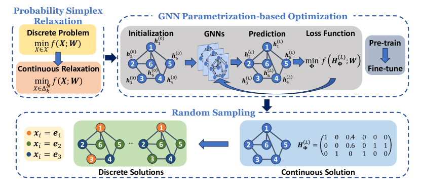
Figure 1: The Relax-Optimize-and-Sample framework.

In this work, we propose a GNN-based Relax-Optimize-and-Sample (ROS) framework for efficiently solving the Max-$k$-Cut problem with arbitrary edge weights. The framework is depicted in Figure 1. Initially, the Max-$k$-Cut problem is formulated as a discrete optimization task. To handle this, we introduce probability simplex relaxations, transforming the discrete problem into a continuous one. We then optimize the relaxed formulation by training parameterized GNNs in an unsupervised manner. To further improve efficiency, we apply transfer learning, utilizing pre-trained GNNs to warm-start the training process. Finally, we refine the continuous solution using a random sampling algorithm, resulting in high-quality Max-$k$-Cut solutions.

The key contributions of our work are summarized as follows:

• Novel Framework. We propose a scalable ROS framework tailored to the weighted Max-$k$-Cut problem with arbitrary signs, built on solving continuous relaxations using efficient learning-based techniques.

• Theoretical Foundations. We conduct a rigorous theoretical analysis of both the relaxation and sampling steps. By integrating geometric landscape analysis with statistical theory, we demonstrate the consistency of function values between the continuous solution and its sampled discrete counterpart.

• Superior Performance. Comprehensive experiments on public benchmark datasets show that our framework produces high-quality solutions for Max-$k$-Cut instances with up to $20,000$ nodes in just a few seconds. Our approach significantly outperforms state-of-the-art algorithms, while also demonstrating strong generalization across various instance types.

2 Preliminaries

2.1 Max-$k$-Cut Problems

Let $\mathcal{G}=(\mathcal{V},\mathcal{E})$ represent an undirected graph with vertex set $\mathcal{V}$ and edge set $\mathcal{E}$. Each edge $(i,j)\in\mathcal{E}$ is assigned an arbitrary weight $\bm{W}_{ij}\in\mathbb{R}$, which can have any sign. A cut in $\mathcal{G}$ refers to a partition of its vertex set. The Max-$k$-Cut problem involves finding a $k$-partition $(\mathcal{V}_{1},\dots,\mathcal{V}_{k})$ of the vertex set $\mathcal{V}$ such that the sum of the weights of the edges between different partitions is maximized.

To represent this partitioning, we employ a $k$-dimensional one-hot encoding scheme. Specifically, we define a $k\times N$ matrix $\bm{X}\in\mathbb{R}^{k\times N}$ where each column represents a one-hot vector. The Max-$k$-Cut problem can be formulated as:

$$\underset{\bm{X}\in\mathbb{R}^{k\times N}}{\text{max}} \frac{1}{2}\sum_{i=1}^{N}\sum_{j=1}^{N}\bm{W}_{ij}\left(1-\bm{X}_{\cdot i}^{\top}\bm{X}_{\cdot j}\right)$$ (1)

   s. t. $$\bm{X}_{\cdot j}\in\{\bm{e}_{1},\bm{e}_{2},\dots,\bm{e}_{k}\}\quad\quad\forall j\in\mathcal{V},$$

where $\bm{X}_{\cdot j}$ denotes the $j^{th}$ column of $\bm{X}$, $\bm{W}$ is a symmetric matrix with zero diagonal entries, and $\bm{e}_{\ell}\in\mathbb{R}^{k}$ is a one-hot vector with the $\ell^{th}$ entry set to $1$. This formulation aims to maximize the total weight of edges between different partitions, ensuring that each node is assigned to exactly one partition, represented by the one-hot encoded vectors. We remark that weighted Max-$k$-Cut problems with arbitrary signs is a generalization of classic Max-Cut problems and arise in many interesting applications (De Simone et al., 1995; Poland & Zeugmann, 2006; Hojny et al., 2021).

2.2 Graph Neural Networks

GNNs are powerful tools for learning representations from graph-structured data. GNNs operate by iteratively aggregating information from a node’s neighbors, enabling each node to capture increasingly larger sub-graph structures as more layers are stacked. This process allows GNNs to learn complex patterns and relationships between nodes, based on their local connectivity.

At the initial layer ($l=0$), each node $i\in\mathcal{V}$ is assigned a feature vector $\bm{h}_{i}^{(0)}$, which typically originates from node features or labels. The representation of node $i$ is then recursively updated at each subsequent layer through a parametric aggregation function $f_{\bm{\Phi}^{(l)}}$, defined as:

$$\bm{h}_{i}^{(l)}=f_{\bm{\Phi}^{(l)}}\left(\bm{h}_{i}^{(l-1)},\{\bm{h}_{j}^{(l-1)}:j\in\mathcal{N}(i)\}\right),$$ (2)

where $\bm{\Phi}^{(l)}$ represents the trainable parameters at layer $l$, $\mathcal{N}(i)$ denotes the set of neighbors of node $i$, and $\bm{h}_{i}^{(l)}$ is the node’s embedding at layer $l$ for $l\in\{1,2,\cdots,L\}$. This iterative process enables the GNN to propagate information throughout the graph, capturing both local and global structural properties.

3 A Relax-Optimize-and-Sample Framework

In this work, we leverage continuous optimization techniques to tackle Max-$k$-Cut problems, introducing a novel ROS framework. Acknowledging the inherent challenges of discrete optimization, we begin by relaxing the problem to probability simplices and concentrate on optimizing this relaxed version. To achieve this, we propose a machine learning-based approach. Specifically, we model the relaxed problem using GNNs, pre-training the GNN on a curated graph dataset before fine-tuning it on the specific target instance. After obtaining high-quality solutions to the relaxed continuous problem, we employ a random sampling procedure to derive a discrete solution that preserves the same objective value.

3.1 Probability Simplex Relaxations

To simplify the formulation of the problem (1), we remove constant terms and negate the objective function, yielding an equivalent formulation expressed as follows:

$$\underset{\bm{X}\in\mathcal{X}}{\text{min}}\quad f(\bm{X};\bm{W})\coloneqq\text{Tr}(\bm{X}\bm{W}\bm{X}^{\top}),\hskip 56.9055pt(\textbf{P})$$

where $\mathcal{X}\coloneqq\left\{\bm{X}\in\mathbb{R}^{k\times N}:\bm{X}_{\cdot j}\in\{\bm{e}_{1},\bm{e}_{2},\dots,\bm{e}_{k}\},\forall j\in\mathcal{V}\right\}$. It is important to note that the matrix $\bm{W}$ is indefinite due to its diagonal entries being set to zero.

Given the challenges associated with solving the discrete problem P, we adopt a naive relaxation approach, obtaining the convex hull of $\mathcal{X}$ as the Cartesian product of $N$ $k$-dimensional probability simplices, denoted by $\Delta_{k}^{N}$. Consequently, the discrete problem P is relaxed into the following continuous optimization form:

$$\underset{\bm{X}\in\Delta_{k}^{N}}{\text{min}} \quad f(\bm{X};\bm{W}).\hskip 56.9055pt(\overline{\textbf{P}})$$

Before optimizing problem $\overline{\textbf{P}}$, we will characterize its geometric landscape. To facilitate this, we introduce the following definition.

Definition 1.

Let $\overline{\bm{X}}$ denote a point in $\Delta_{k}^{N}$. We define the neighborhood induced by $\overline{\bm{X}}$ as follows:

$$\mathcal{N}(\overline{\bm{X}})\coloneqq\left\{\bm{X}\in\Delta_{k}^{N}\left|\begin{aligned} &\sum_{i\in\mathcal{K}(\overline{\bm{X}}_{\cdot j})}\bm{X}_{ij}=1,&&\forall j\in\mathcal{V}\end{aligned}\right.\right\},$$

where $\mathcal{K}(\overline{\bm{X}}_{\cdot j})\coloneqq\{i\in\{1,\ldots,k\}\mid\overline{\bm{X}}_{ij}>0\}$.

The set $\mathcal{N}(\overline{\bm{X}})$ represents a neighborhood around $\overline{\bm{X}}$, where each point in $\mathcal{N}(\overline{\bm{X}})$ can be derived by allowing each non-zero entry of the matrix $\overline{\bm{X}}$ to vary freely, while the other entries are set to zero. Utilizing this definition, we can establish the following theorem.

Theorem 1.

Let $\overline{\bm{X}}$ denote a globally optimal solution to $\overline{\textbf{P}}$, and let $\mathcal{N}(\overline{\bm{X}})$ be its induced neighborhood. Then

$$f(\bm{X};\bm{W})=f(\overline{\bm{X}};\bm{W}), \forall\bm{X}\in\mathcal{N}(\overline{\bm{X}}).$$

Theorem 1 states that for a globally optimal solution $\overline{\bm{X}}$, every point within its neighborhood $\mathcal{N}(\overline{\bm{X}})$ shares the same objective value as $\overline{\bm{X}}$, thus forming a basin in the geometric landscape of $f(\bm{X};\bm{W})$. If $\overline{\bm{X}}\in\mathcal{X}$ (i.e., an integer solution), then $\mathcal{N}(\overline{\bm{X}})$ reduces to the singleton set $\left\{\overline{\bm{X}}\right\}$. Conversely, if $\overline{\bm{X}}\notin\mathcal{X}$, there exist $\prod_{j\in\mathcal{V}}|\mathcal{K}(\overline{\bm{X}}_{\cdot j})|$ unique integer solutions within $\mathcal{N}(\overline{\bm{X}})$ that maintain the same objective value as $\overline{\bm{X}}$. This indicates that once a globally optimal solution to the relaxed problem $\overline{\textbf{P}}$ is identified, it becomes straightforward to construct an optimal solution for the original problem P that preserves the same objective value.

According to Carlson & Nemhauser (1966), among all globally optimal solutions to the relaxed problem $\overline{\textbf{P}}$, there is always at least one integer solution. Theorem 1 extends this result, indicating that if the globally optimal solution is fractional, we can provide a straightforward and efficient method to derive its integer counterpart. We remark that it is highly non-trivial to guarantee that the feasible Max-$k$-Cut solution obtained from the relaxation one has the same quality.

Example. Consider a Max-Cut problem ($k=2$) associated with the weight matrix $\bm{W}$. We optimize its relaxation and obtain the optimal solution $\bm{X}^{\star}$.

$$\bm{W}\coloneqq\begin{pmatrix}0&1&1\\ 1&0&1\\ 1&1&0\end{pmatrix},\bm{X}^{\star}\coloneqq\begin{pmatrix}p&1&0\\ 1-p&0&1\end{pmatrix},$$

where $p\in\left[0,1\right]$. From the neighborhood $\mathcal{N}(\overline{\bm{X}})$, We can identify the following integer solutions that maintain the same objective value.

$$\bm{X}_{1}^{\star}=\begin{pmatrix}0&1&0\\ 1&0&1\end{pmatrix},\bm{X}_{2}^{\star}=\begin{pmatrix}1&1&0\\ 0&0&1\end{pmatrix}.$$

Given that $\overline{\textbf{P}}$ is a non-convex program, identifying its global minimum is challenging. Consequently, the following two critical questions arise.

• Since solving $\overline{\textbf{P}}$ to global optimality is $\mathcal{NP}$-hard, how to efficiently optimize $\overline{\textbf{P}}$ for high-quality solutions?

• Given $\overline{\bm{X}}\in\Delta_{k}^{N}\setminus\mathcal{X}$ as a high-quality solution to $\overline{\textbf{P}}$, can we construct a feasible solution $\hat{\bm{X}}\in\mathcal{X}$ to P such that $f(\hat{\bm{X}};\bm{W})=f(\overline{\bm{X}};\bm{W})$?

We provide a positive answer to Q2 in Section 3.2, while our approach to addressing Q1 is deferred to Section 3.3.

3.2 Random Sampling

Let $\overline{\bm{X}}\in\Delta_{k}^{N}\setminus\mathcal{X}$ be a feasible solution to the relaxation $\overline{\textbf{P}}$. Our goal is to construct a feasible solution $\bm{X}\in\mathcal{X}$ for the original problem P, ensuring that the corresponding objective values are equal. Inspired by Theorem 1, we propose a random sampling procedure, outlined in Algorithm 1. In this approach, we sample each column $\bm{X}_{\cdot i}$ of the matrix $\bm{X}$ from a categorical distribution characterized by the event probabilities $\overline{\bm{X}}_{\cdot i}$ (denoted as $\text{Cat}(\bm{x};\bm{p}=\overline{\bm{X}}_{\cdot i})$ in Step 3 of Algorithm 1). This randomized approach yields a feasible solution $\hat{\bm{X}}$ for P. However, since Algorithm 1 incorporates randomness in generating $\hat{\bm{X}}$ from $\overline{\bm{X}}$, the value of $f(\hat{\bm{X}};\bm{W})$ becomes random as well. This raises the critical question: is this value greater or lesser than $f(\overline{\bm{X}};\bm{W})$? We address this question in Theorem 2.

Algorithm 1 Random Sampling

1:Input: $\overline{\bm{X}}\in\Delta_{k}^{N}$ $\triangleright$ any feasible solution to $\overline{\bm{P}}$

2:for $i=1$ to $N$ do $\triangleright$ each dimension is independent

3:     $\hat{\bm{X}}_{\cdot i}\sim\text{Cat}(\bm{x};\bm{p}=\overline{\bm{X}}_{\cdot i})$ $\triangleright$ sampling from a categorical distribution

4:end for

5:Output: $\hat{\bm{X}}\in\mathcal{X}$ $\triangleright$ a feasible solution to $\bm{P}$

Theorem 2.

Let $\overline{\bm{X}}$ and $\hat{\bm{X}}$ denote the input and output of Algorithm 1, respectively. Then, we have $\mathbb{E}_{\hat{\bm{X}}}[f(\hat{\bm{X}};\bm{W})]=f(\overline{\bm{X}};\bm{W})$.

Theorem 2 states that $f(\hat{\bm{X}};\bm{W})$ is equal to $f(\overline{\bm{X}};\bm{W})$ in expectation. This implies that the random sampling procedure operates on a fractional solution, yielding Max-$k$-Cut feasible solutions with the same objective values in a probabilistic sense. While the Lovász-extension-based method (Bach et al., 2013) also offers a framework for continuous relaxation, achieving similar theoretical results for arbitrary $k$ and edge weights $\bm{W}_{i,j}\in\mathbb{R}$ is not always guaranteed. In practice, we execute Algorithm 1 $T$ times and select the solution with the lowest objective value as our best result. We remark that the theoretical interpretation in Theorem 2 distinguishes our sampling algorithm from the existing ones in the literature (Toenshoff et al., 2021; Karalias & Loukas, 2020).

3.3 GNN Parametrization-Based Optimization

To solve the problem $\overline{\textbf{P}}$, we propose an efficient learning-to-optimize (L2O) method based on GNN parametrization. This approach reduces the laborious iterations typically required by classical optimization methods (e.g., mirror descent). Additionally, we introduce a “pre-train + fine-tune” strategy, where the model is endowed with prior graph knowledge during the pre-training phase, significantly decreasing the computational time required to optimize $\overline{\textbf{P}}$.

GNN Parametrization. The Max-$k$-Cut problem can be framed as a node classification task, allowing us to leverage GNNs to aggregate node features, and obtain high-quality solutions. Initially, we assign a random embedding $\bm{h}_{i}^{(0)}$ to each node $i$ in the graph $\mathcal{G}$, as defined in Section 2. We adopt the GNN architecture proposed by Morris et al. (2019), utilizing an $L$-layer GNN with updates at layer $l$ defined as follows:

$$\bm{h}_{i}^{(l)}\coloneqq\sigma\left(\bm{\Phi}_{1}^{(l)}\bm{h}_{i}^{(l-1)}+\bm{\Phi}_{2}^{(l)}\sum_{j\in\mathcal{N}(i)}w_{ji}\bm{h}_{j}^{(l-1)}\right),$$

where $\sigma(\cdot)$ is an activation function, and $\bm{\Phi}_{1}^{(l)}$ and $\bm{\Phi}_{2}^{(l)}$ are the trainable parameters at layer $l$ for $l\in\{1,\dots,L\}$. This formulation facilitates efficient learning of node representations by leveraging both node features and the underlying graph structure. After processing through $L$ layers of GNN, we obtain the final output $\bm{H}^{(L)}_{\bm{\Phi}}\coloneqq[\bm{h}_{1}^{(L)},\dots,\bm{h}_{N}^{(L)}]\in\mathbb{R}^{k\times N}$. A softmax activation function is then applied in the last layer to ensure $\bm{H}^{(L)}_{\bm{\Phi}}\in\Delta_{k}^{N}$, making the final output feasible for $\overline{\bm{P}}$.

“Pre-train + Fine-tune” Optimization. We propose a “pre-train + fine-tune” framework for learning the trainable weights of GNNs. Initially, the model is trained on a collection of pre-collected datasets to produce a pre-trained model. Subsequently, we fine-tune this pre-trained model for each specific problem instance. This approach equips the model with prior knowledge of graph structures during the pre-training phase, significantly reducing the overall solving time. Furthermore, it allows for out-of-distribution generalization due to the fine-tuning step.

The trainable parameters $\bm{\Phi}\coloneqq(\bm{\Phi}_{1}^{(1)},\bm{\Phi}_{2}^{(1)},\dots,\bm{\Phi}_{1}^{(L)},\bm{\Phi}_{2}^{(L)})$ in the pre-training phase are optimized using the Adam optimizer with random initialization, targeting the objective

$$\min_{\bm{\Phi}}\quad\mathcal{L}_{\text{pre-training}}(\bm{\Phi})\coloneqq\frac{1}{M}\sum_{m=1}^{M}f(\bm{H}_{\Phi}^{(L)};\bm{W}_{\text{train}}^{(m)}),$$

where $\mathcal{D}\coloneqq\{\bm{W}_{\text{train}}^{(1)},\dots,\bm{W}_{\text{train}}^{(M)}\}$ represents the pre-training dataset. In the fine-tuning phase, for a problem instance represented by $\bm{W}_{\text{test}}$, the Adam optimizer seeks to solve

$$\min_{\bm{\Phi}}\quad\mathcal{L}_{\text{fine-tuning}}(\bm{\Phi})\coloneqq f(\bm{H}_{\Phi}^{(L)};\bm{W}_{\text{test}}),$$

initialized with the pre-trained parameters.

Moreover, to enable the GNN model to fully adapt to specific problem instances, the pre-training phase can be omitted, enabling the model to be directly trained and tested on the same instance. While this direct approach may necessitate more computational time, it often results in improved performance regarding the objective function. Consequently, users can choose to include a pre-training phase based on the specific requirements of their application scenarios.

4 Experiments

4.1 Experimental Settings

We compare the performance of ROS against traditional methods and L2O algorithms for solving the Max-$k$-Cut problem. Additionally, we assess the impact of the “Pre-train” stage in the GNN parametrization-based optimization. The source code is available at https://anonymous.4open.science/r/ROS_anonymous-1C88/.

Baseline Algorithms. We denote our proposed algorithms by ROS and compare them against both traditional algorithms and learning-based methods. When the pre-training step is skipped, we refer to our algorithm as ROS-vanilla. The following traditional Max-$k$-Cut algorithms are considered as baselines: (i) GW (Goemans & Williamson, 1995): an method with a $0.878$-approximation guarantee based on semi-definite relaxation; (ii) BQP (Gui et al., 2018): a local search method designed for binary quadratic programs; (iii) Genetic (Li & Wang, 2016): a genetic algorithm specifically for Max-$k$-Cut problems; (iv) MD: a mirror descent algorithm that addresses the relaxed problem $\overline{\textbf{P}}$ with a convergence tolerance at $10^{-8}$ and adopts the same random sampling procedure; (v) LPI (Goudet et al., 2024): an evolutionary algorithm featuring a large population organized across different islands; (vi) MOH (Ma & Hao, 2017): a heuristic algorithm based on multiple operator heuristics, employing various distinct search operators within the search phase. (vii) Rank2 (Burer et al., 2002): a heuristic based on rank-2 relaxation. For the L2O method, we primarily examine the state-of-the-art baseline: (viii) PI-GNN (Schuetz et al., 2022): A cutting-edge L2O method capable of solving QUBO problems in dozens of seconds, delivering commendable performance. It is the first method to eliminate the dependence on large, labeled training datasets typically required by supervised learning approaches.

Datasets. The datasets utilized in this paper comprise random regular graphs from Schuetz et al. (2022) and the Gset benchmark from Ye (2003). For the random regular graphs, we employ the random_regular_graph from the NetworkX library (Hagberg et al., 2008) to generate $r$-regular graphs, which are undirected graphs in which all nodes have a degree of $r$, with all edge weights equal to $1$. The Gset benchmark is constructed using a machine-independent graph generator, encompassing toroidal, planar, and randomly weighted graphs with vertex counts ranging from $800$ to $20,000$ and edge densities between $2\%$ and $6\%$. The edge weights in these graphs are constrained to values of $1$, $0$, or $-1$. Specifically, the training dataset includes $500$ $3$-regular graphs and $500$ $5$-regular graphs, each containing $100$ nodes, tailored for the cases where $k=2$ and $k=3$, respectively. The testing set for random regular graphs consists $20$ $3$-regular graphs and $20$ $5$-regular graphs for both $k=2$ and $k=3$ tasks, with node counts of $100$, $1,000$, and $10,000$, respectively. Moreover, the testing set of Gset encompasses all instances included in the Gset benchmark.

Model Settings. ROS is designed as a two-layer GNN, with both the input and hidden dimensions set to $100$. To address the issue of gradient vanishing, we apply a graph normalization technique as proposed by Cai et al. (2021). The ROS model undergoes pre-training using the Adam optimizer with a learning rate of $10^{-2}$ for one epoch. During the fine-tuning stage, the model is further optimized using the same Adam optimizer and learning rate of $10^{-2}$. An early stopping strategy is employed, with a tolerance of $10^{-2}$ and a patience of $100$ iterations, terminating training if no improvement is observed over this duration. Finally, in the random sampling stage, we execute Algorithm 1 for $T=100$ independent trials and return the best solution obtained.

Evaluation Configuration. All our experiments were conducted on an NVIDIA RTX 3090 GPU, using Python 3.8.19 and PyTorch 2.2.0.

4.2 Performance Comparison against Baselines

4.2.1 Computational Time

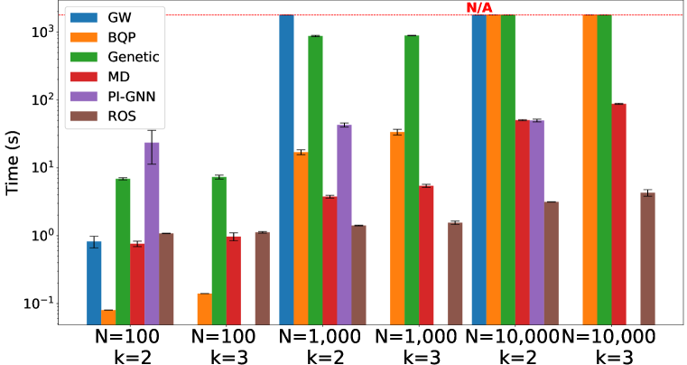
(a) Random Regular Graph

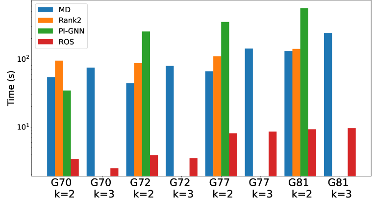
(b) Gset

Figure 2: The computational time comparison of Max-$k$-Cut problems.

We evaluated the performance of ROS against baseline algorithms GW, BQP, Genetic, MD, and PI-GNN on random regular graphs, focusing on computational time for both the Max-Cut and Max-3-Cut tasks. The experiments were conducted across three problem sizes: $N=100$, $N=1{,}000$, and $N=10{,}000$, as illustrated in Figure 2(a). Additionally, Figure 2(b) compares the scalable methods MD, Rank2, and PI-GNN on problem instances from the Gset benchmark with $N\geq 10{,}000$. “N/A” denotes a failure to return a solution within $30$ minutes. A comprehensive summary of the results for all Gset instances on Max-Cut and Max-$3$-Cut, including comparisons with state-of-the-art methods LPI and MOH, is presented in Table 3 and Table 4 in the Appendix.

The results depicted in Figure 2(a) indicate that ROS efficiently solves all problem instances within seconds, even for large problem sizes of $N=10,000$. In terms of baseline performance, the approximation algorithm GW performs efficiently on instances with $N=100$, but it struggles with larger sizes such as $N=1,000$ and $N=10,000$ due to the substantial computational burden associated with solving the underlying semi-definite programming problem. Heuristic methods such as BQP and Genetic can manage cases up to $N=1,000$ in a few hundred seconds, yet they fail to solve larger instances with $N=10,000$ because of the high computational cost of each iteration. Notably, MD is the only method capable of solving large instances within a reasonable time frame; however, when $N$ reaches $10,000$, the computational time for MD approaches $15$ times that of ROS. Regarding learning-based methods, PI-GNN necessitates retraining and prediction for each test instance, with test times exceeding dozens of seconds even for $N=100$. In contrast, ROS solves these large instances in merely a few seconds. Throughout the experiments, ROS consistently completes its tasks in under $10$ seconds, requiring only $10\%$ of the computational time utilized by PI-GNN. Figure 2(b) illustrates the results for the Gset benchmark, where ROS efficiently solves the largest instances in just a few seconds, while other methods, such as Rank2, take tens to hundreds of seconds for equivalent tasks. Remarkably, ROS utilizes only about $1\%$ of the computational time required by PI-GNN.

4.2.2 Objective Value

Table 1: Objective value comparison of Max-$k$-Cut problems on random regular graphs.

Methods	N=100		N=1,000		N=10,000
	$k=2$	$k=3$	$k=2$	$k=3$	$k=2$	$k=3$
GW	$130.20_{\pm 2.79}$	–	N/A	–	N/A	–
BQP	$131.55_{\pm 2.42}$	$239.70_{\pm 1.82}$	$1324.45_{\pm 6.34}$	$2419.15_{\pm 6.78}$	N/A	N/A
Genetic	$127.55_{\pm 2.82}$	$235.50_{\pm 3.15}$	$1136.65_{\pm 10.37}$	$2130.30_{\pm 8.49}$	N/A	N/A
MD	$127.20_{\pm 2.16}$	$235.50_{\pm 3.29}$	$1250.35_{\pm 11.21}$	$2344.85_{\pm 9.86}$	$12428.85_{\pm 26.13}$	$23341.20_{\pm 32.87}$
PI-GNN	$122.75_{\pm 4.36}$	–	$1263.95_{\pm 21.59}$	–	$12655.05_{\pm 94.25}$	–
ROS	$128.20_{\pm 2.82}$	$240.30_{\pm 2.59}$	$1283.75_{\pm 6.89}$	$2405.75_{\pm 5.72}$	$12856.85_{\pm 26.50}$	$24085.95_{\pm 21.88}$

Table 2: Objective value comparison of Max-$k$-Cut problems on Gset instances.

Methods	G70 (N=10,000)		G72 (N=10,000)		G77 (N=14,000)		G81 (N=20,000)
	$k=2$	$k=3$	$k=2$	$k=3$	$k=2$	$k=3$	$k=2$	$k=3$
MD	$8551$	$9728$	$5638$	$6612$	$7934$	$9294$	$11226$	$13098$
Rank2	$9529$	–	$6820$	–	$9670$	–	$13662$	–
PI-GNN	$8956$	–	$4544$	–	$6406$	–	$8970$	–
ROS	$8916$	$9971$	$6102$	$7297$	$8740$	$10329$	$12332$	$14464$

We also evaluate the performance of ROS on random regular graphs and the Gset benchmark concerning the objective values of Problem (1). The results for the random regular graphs and Gset are presented in Tables 1 and 2, respectively. Note that “–” indicates that the method is unable to handle Max-$k$-Cut problems.

The results for random regular graphs, presented in Table 1, indicate that ROS effectively addresses both $k=2$ and $k=3$ cases, producing high-quality solutions even for large-scale problem instances. In contrast, traditional methods such as GW and the L2O method PI-GNN are restricted to $k=2$ and fail to generalize to the general $k$, i.e., $k=3$. While GW achieves high-quality solutions for the Max-Cut problem with an instance size of $N=100$, it cannot generalize to arbitrary $k$ without integrating additional randomized algorithms to yield discrete solutions. Similarly, the L2O method PI-GNN cannot manage $k=3$ because the Max-$k$-Cut problem cannot be modeled as a QUBO problem. Furthermore, its heuristic rounding lacks theoretical guarantees, which results in sub-optimal performance regarding objective function values. Traditional methods such as BQP and Genetic can accommodate $k=3$, but they often become trapped in sub-optimal solutions. Among all the baselines, only MD can handle general $k$ while producing solutions of comparable quality to ROS. However, MD consistently exhibits inferior performance compared to ROS across all experiments. The results for the Gset benchmark, shown in Table 2, offer similar insights: ROS demonstrates better generalizability compared to the traditional Rank2 method and the L2O method PI-GNN. Moreover, ROS yields higher-quality solutions than MD in terms of objective function values.

4.3 Effect of the “Pre-train” Stage in ROS

To evaluate the impact of the pre-training stage in ROS, we compared it with ROS-vanilla, a variant that omits the pre-training phase (see Section 3.3). We assessed both methods based on objective function values and computational time. Figure 3 illustrates the ratios of these metrics between ROS-vanilla and ROS. In this figure, the horizontal axis represents the problem instances, while the left vertical axis (green bars) displays the ratio of objective function values, and the right vertical axis (red curve) indicates the ratio of computational times.

As shown in Figure 3(a), during experiments on regular graphs, ROS-vanilla achieves higher objective function values in most settings; however, its computational time is approximately $1.5$ times greater than that of ROS. Thus, ROS demonstrates a faster solving speed compared to ROS-vanilla. Similarly, in experiments conducted on the Gset benchmark (Figure 3(b)), ROS reduces computational time by around $40\%$ while maintaining performance comparable to that of ROS-vanilla. Notably, in the Max-3-Cut problem for the largest instance, G81, ROS effectively halves the solving time, showcasing the significant acceleration effect of pre-training. It is worth mentioning that the ROS model was pre-trained on random regular graphs with $N=100$ and generalized well to regular graphs with $N=1{,}000$ and $N=10{,}000$, as well as to Gset problem instances of varying sizes and types. This illustrates ROS’s capability to generalize and accelerate the solving of large-scale problems across diverse graph types and sizes, emphasizing the strong out-of-distribution generalization afforded by pre-training.

In summary, while ROS-vanilla achieves slightly higher objective function values on individual instances, it requires longer solving times and struggles to generalize to other problem instances. This observation highlights the trade-off between a model’s ability to generalize and its capacity to fit specific instances. Specifically, a model that fits individual instances exceptionally well may fail to generalize to new data, resulting in longer solving times. Conversely, a model that generalizes effectively may exhibit slightly weaker performance on specific instances, leading to a marginal decrease in objective function values. Therefore, the choice between these two training modes should be guided by the specific requirements of the application.

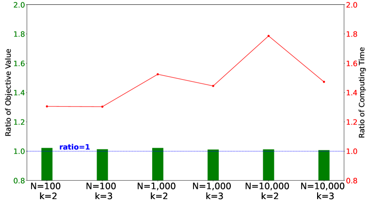
(a) Random regular graph

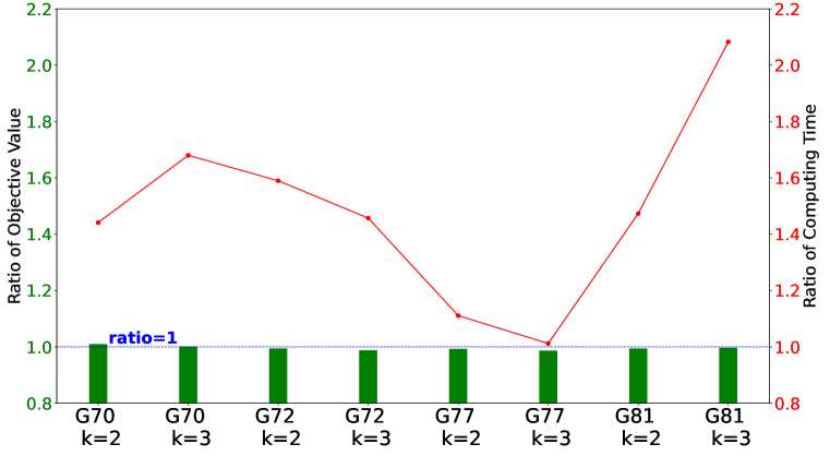
(b) Gset

Figure 3: The ratio of computational time and objective value comparison of Max-$k$-Cut problems between ROS-vanilla and ROS.

5 Conclusions

In this paper, we propose ROS, an efficient method for addressing the Max-$k$-Cut problem with any arbitrary edge weights. Our approach begins by relaxing the constraints of the original discrete problem to probabilistic simplices. To effectively solve this relaxed problem, we propose an optimization algorithm based on GNN parametrization and incorporate transfer learning by leveraging pre-trained GNNs to warm-start the training process. After resolving the relaxed problem, we present a novel random sampling algorithm that maps the continuous solution back to a discrete form. By integrating geometric landscape analysis with statistical theory, we establish the consistency of function values between the continuous and discrete solutions. Experiments conducted on random regular graphs and the Gset benchmark demonstrate that our method is highly efficient for solving large-scale Max-$k$-Cut problems, requiring only a few seconds, even for instances with tens of thousands of variables. Furthermore, it exhibits robust generalization capabilities across both in-distribution and out-of-distribution instances, highlighting its effectiveness for large-scale optimization tasks. Exploring other sampling algorithms to further boost ROS performance is a future research direction. Moreover, the ROS framework with theoretical insights could be potentially extended to other graph-related combinatorial problems, and this direction is also worth investigating as future work.

Appendix A Proof of Theorem 1

Proof.

Before proceeding with the proof of Theorem 1, we first define the neighborhood of a vector $\bar{\bm{x}}\in\Delta_{k}$, and establish results of Lemma 1 and Lemma 2.

Definition 2.

Let $\bar{\bm{x}}=(\bar{\bm{x}}_{1},\cdots,\bar{\bm{x}}_{k})$ denote a point in $\Delta_{k}$. We define the neighborhood induced by $\bar{\bm{x}}$ as follows:

$$\widetilde{\mathcal{N}}(\bar{\bm{x}})\coloneqq\left\{(\bm{x}_{1},\cdots,\bm{x}_{k})\in\Delta_{k}\left|\sum_{j\in\mathcal{K}(\bar{\bm{x}})}\bm{x}_{j}=1\right.\right\},$$

where $\mathcal{K}(\bar{\bm{x}})=\left\{j\in\{1,\cdots,k\}\mid\bar{\bm{x}}_{j}>0\right\}$.

Lemma 1.

Given $\bm{X}_{\cdot i}\in\widetilde{\mathcal{N}}(\overline{\bm{X}}_{\cdot i})$, it follows that

$$\mathcal{K}(\bm{X}_{\cdot i})\subseteq\mathcal{K}(\overline{\bm{X}}_{\cdot i}).$$

Proof.

Suppose there exists $j\in\mathcal{K}(\bm{X}_{\cdot i})$ such that $j\notin\mathcal{K}(\overline{\bm{X}}_{\cdot i})$, implying $\bm{X}_{ji}>0$ and $\overline{\bm{X}}_{ji}=0$.

We then have

$$\sum_{l\in\mathcal{K}(\overline{\bm{X}}_{\cdot i})}\bm{X}_{li}+\bm{X}_{ji}\leq\sum_{l=1}^{k}\bm{X}_{li}=1,$$

which leads to

$$\sum_{l\in\mathcal{K}(\overline{\bm{X}}_{\cdot i})}\bm{X}_{li}\leq 1-\bm{X}_{ji}<1,$$

contradicting with the fact that $\bm{X}_{\cdot i}\in\widetilde{\mathcal{N}}(\overline{\bm{X}}_{\cdot i})$. ∎

Lemma 2.

Let $\overline{\bm{X}}$ be a globally optimal solution to $\overline{\textbf{P}}$, then

$$f(\bm{X};\bm{W})=f(\overline{\bm{X}};\bm{W}),$$

where $\bm{X}$ has only the $i^{th}$ column $\bm{X}_{\cdot i}\in\widetilde{\mathcal{N}}(\overline{\bm{X}}_{\cdot i})$, and other columns are identical to those of $\overline{\bm{X}}$. Moreover, $\bm{X}$ is also a globally optimal solution to $\bar{\bm{P}}$.

Proof.

The fact that $\bm{X}$ is a globally optimal solution to $\bar{\bm{P}}$ follows directly from the equality $f(\bm{X};\bm{W})=f(\overline{\bm{X}};\bm{W})$. Thus, it suffices to prove this equality. Consider that $\overline{\bm{X}}$ and $\bm{X}$ differ only in the $i^{th}$ column, and $\bm{X}_{\cdot i}\in\widetilde{\mathcal{N}}(\overline{\bm{X}}_{\cdot i})$. We can rewrite the objective value function as

$$f(\bm{X};\bm{W})=g(\bm{X}_{\cdot i};\bm{X}_{\cdot-i})+h(\bm{X}_{\cdot-i}),$$

where $\bm{X}_{\cdot-i}$ represents all column vectors of $\bm{X}$ except the $i^{th}$ column. The functions $g$ and $h$ are defined as follows:

$$g(\bm{X}_{\cdot i};\bm{X}_{\cdot-i}) =\sum_{j=1}^{N}\bm{W}_{ij}\bm{X}_{\cdot i}^{\top}\bm{X}_{\cdot j}+\sum_{j=1}^{N}\bm{W}_{ji}\bm{X}_{\cdot j}^{\top}\bm{X}_{\cdot i}-\bm{W}_{ii}\bm{X}_{\cdot i}^{\top}\bm{X}_{\cdot i},$$

$$h(\bm{X}_{\cdot-i}) =\sum_{l=1,l\neq i}^{N}\sum_{j=1,j\neq i}^{N}\bm{W}_{lj}\bm{X}_{\cdot l}^{\top}\bm{X}_{\cdot j}$$

To establish that $f(\bm{X};\bm{W})=f(\overline{\bm{X}};\bm{W})$, it suffices to show that

$$g(\bm{X}_{\cdot i};\bm{X}_{\cdot-i})=g(\overline{\bm{X}}_{\cdot i};\bm{X}_{\cdot-i})$$

as $\bm{X}_{\cdot-i}=\overline{\bm{X}}_{\cdot-i}$.

Rewriting $g(\bm{X}_{\cdot i};\bm{X}_{\cdot-i})$, we obtain

$$g(\bm{X}_{\cdot i};\bm{X}_{\cdot-i}) =\sum_{j=1}^{N}\bm{W}_{ij}\bm{X}_{\cdot i}^{\top}\bm{X}_{\cdot j}+\sum_{j=1}^{N}\bm{W}_{ji}\bm{X}_{\cdot j}^{\top}\bm{X}_{\cdot i}$$

$$=2\sum_{j=1}^{N}\bm{W}_{ij}\bm{X}_{\cdot i}^{\top}\bm{X}_{\cdot j}$$

$$=2\bm{X}_{\cdot i}^{\top}\sum_{j=1,j\neq i}^{N}\bm{W}_{ij}\bm{X}_{\cdot j}$$

$$=2\bm{X}_{\cdot i}^{\top}\bm{Y}_{\cdot i},$$

where $\bm{Y}_{\cdot i}:=\sum_{j=1,j\neq i}^{N}\bm{W}_{ij}\bm{X}_{\cdot j}$.

If $|\mathcal{K}(\overline{\bm{X}}_{\cdot i})|=1$, then there is only one non-zero element in $\overline{\bm{X}}_{\cdot i}$ equal to one. Therefore, $g(\overline{\bm{X}}_{\cdot i};\bm{X}_{\cdot-i})=g(\bm{X}_{\cdot i};\bm{X}_{\cdot-i})$ since $\bm{X}_{\cdot i}=\overline{\bm{X}}_{\cdot i}$.

For the case where $|\mathcal{K}(\overline{\bm{X}}_{\cdot i})|>1$, we consider any indices $j,l\in\mathcal{K}(\overline{\bm{X}}_{\cdot i})$ such that $\overline{\bm{X}}_{ji},\overline{\bm{X}}_{li}>0$. Then, there exists $\epsilon>0$ such that we can construct a point $\widetilde{\bm{x}}\in\Delta_{k}$ where the $j^{th}$ element is set to $\overline{\bm{X}}_{ji}-\epsilon$, the $l^{th}$ element is set to $\overline{\bm{X}}_{li}+\epsilon$, and all other elements remain the same as in $\overline{\bm{X}}_{\cdot i}$. Since $\overline{\bm{X}}$ is a globally optimum of the function $f(\bm{X};\bm{W})$, it follows that $\overline{\bm{X}}_{\cdot i}$ is also a global optimum for the function $g(\overline{\bm{X}}_{\cdot i};\bm{X}_{\cdot-i})$. Thus, we have

$$g(\overline{\bm{X}}_{\cdot i};\bm{X}_{\cdot-i}) \leq g(\widetilde{\bm{x}};\bm{X}_{\cdot-i})$$

$$\overline{\bm{X}}_{\cdot i}^{\top}\bm{Y}_{\cdot i} \leq\widetilde{\bm{x}}^{\top}\bm{Y}_{\cdot i}$$

$$=\overline{\bm{X}}_{\cdot i}^{\top}\bm{Y}_{\cdot i}-\epsilon\bm{Y}_{ji}+\epsilon\bm{Y}_{li},$$

which leads to the inequality

$$\bm{Y}_{ji}\leq\bm{Y}_{li}.$$ (3)

Next, we can similarly construct another point $\hat{\bm{x}}\in\Delta_{k}$ with its $j^{th}$ element equal to $\overline{\bm{X}}_{ji}+\epsilon$, the $k^{th}$ element equal to $\overline{\bm{X}}_{ki}-\epsilon$, and all other elements remain the same as in $\overline{\bm{X}}_{\cdot i}$. Subsequently, we can also derive that

$$g(\overline{\bm{X}}_{\cdot i};\bm{X}_{\cdot-i}) \leq g(\hat{\bm{x}};\bm{X}_{\cdot-i})$$

$$=\overline{\bm{X}}_{\cdot i}^{\top}\bm{Y}_{\cdot i}+\epsilon\bm{Y}_{ji}-\epsilon\bm{Y}_{li},$$

which leads to another inequality

$$\bm{Y}_{li}\leq\bm{Y}_{ji}.$$ (4)

Consequently, combined inequalities (3) and (4), we have

$$\bm{Y}_{ji}=\bm{Y}_{li},$$

for $j,l\in\mathcal{K}(\overline{\bm{X}}_{\cdot i})$.

From this, we can deduce that

$$\bm{Y}_{j_{1}i}=\bm{Y}_{j_{2}i}=\cdots=\bm{Y}_{j_{|\mathcal{K}(\overline{\bm{X}}_{\cdot i})|}i}=t,$$

where $j_{1},\cdots,j_{|\mathcal{K}(\overline{\bm{X}}_{\cdot i})|}\in\mathcal{K}(\overline{\bm{X}}_{\cdot i})$.

Next, we find that

$$g(\overline{\bm{X}}_{\cdot i};\bm{X}_{\cdot-i}) =2\overline{\bm{X}}_{\cdot i}^{\top}\bm{Y}_{\cdot i}$$

$$=2\sum_{j=1}^{k}\overline{\bm{X}}_{ji}\bm{Y}_{ji}$$

$$=2\sum_{j=1,j\in\mathcal{K}(\overline{\bm{X}}_{\cdot i})}^{N}\overline{\bm{X}}_{ji}\bm{Y}_{ji}$$

$$=2t\sum_{j=1,j\in\mathcal{K}(\overline{\bm{X}}_{\cdot i})}^{N}\overline{\bm{X}}_{ji}$$

$$=2t.$$

Similarly, we have

$$g(\bm{X}_{\cdot i};\bm{X}_{\cdot-i}) =2\bm{X}_{\cdot i}^{\top}\bm{Y}_{\cdot i}$$

$$=2\sum_{j=1}^{k}\bm{X}_{ji}\bm{Y}_{ji}$$

$$=2\sum_{j=1,j\in\mathcal{K}(\bm{X}_{\cdot i})}\bm{X}_{ji}\bm{Y}_{ji}$$

$$\overset{\text{Lemma \ref{lemma1}}}{=}2t\sum_{j=1,j\in\mathcal{K}(\bm{X}_{\cdot i})}\bm{X}_{ji}$$

$$=2t$$

$$=g(\overline{\bm{X}}_{\cdot i})$$

Accordingly, we conclude that

$$g(\bm{X}_{\cdot i};\bm{X}_{\cdot-i})=g(\overline{\bm{X}}_{\cdot i};\bm{X}_{\cdot-i}),$$

which leads us to the result

$$f(\bm{X};\bm{W})=f(\overline{\bm{X}};\bm{W}),$$

where $\bm{X}_{\cdot i}\in\widetilde{\mathcal{N}}(\overline{\bm{X}}_{\cdot i})$, $\bm{X}_{\cdot-i}=\overline{\bm{X}}_{\cdot-i}$. ∎

Accordingly, for any $\bm{X}\in\mathcal{N}(\overline{\bm{X}})$, we iteratively apply Lemma 2 to each column of $\overline{\bm{X}}$ while holding the other columns fixed, thereby proving Theorem 1.

∎

Appendix B Proof of Theorem 2

Proof.

Based on $\overline{\bm{X}}$, we can construct the random variable $\widetilde{\bm{X}}$, where $\widetilde{\bm{X}}_{\cdot i}\sim\text{Cat}(\bm{x};\bm{p}=\overline{\bm{X}}_{\cdot i})$. The probability mass function is given by

$$\textbf{P}(\widetilde{\bm{X}}_{\cdot i}=\bm{e}_{\ell})=\overline{\bm{X}}_{\ell i},$$ (5)

where $\ell=1,\cdots,k$.

Next, we have

$$\mathbb{E}_{\widetilde{\bm{X}}}[f(\widetilde{\bm{X}};\bm{W})] =\mathbb{E}_{\widetilde{\bm{X}}}[\widetilde{\bm{X}}\bm{W}\widetilde{\bm{X}}^{\top}]=\mathbb{E}_{\widetilde{\bm{X}}}[\sum_{i=1}^{N}\sum_{j=1}^{N}\bm{W}_{ij}\widetilde{\bm{X}}_{\cdot i}^{\top}\widetilde{\bm{X}}_{\cdot j}]$$

$$=\sum_{i=1}^{N}\sum_{j=1}^{N}\bm{W}_{ij}\mathbb{E}_{\widetilde{\bm{X}}_{\cdot i}\widetilde{\bm{X}}_{\cdot j}}[\widetilde{\bm{X}}_{\cdot i}^{\top}\widetilde{\bm{X}}_{\cdot j}]$$

$$=\sum_{i=1}^{N}\sum_{j=1}^{N}\bm{W}_{ij}\mathbb{E}_{\widetilde{\bm{X}}_{\cdot i}\widetilde{\bm{X}}_{\cdot j}}[\mathbbm{1}(\widetilde{\bm{X}}_{\cdot i}=\widetilde{\bm{X}}_{\cdot j})]$$

$$=\sum_{i=1}^{N}\sum_{j=1}^{N}\bm{W}_{ij}\mathbb{P}(\widetilde{\bm{X}}_{\cdot i}=\widetilde{\bm{X}}_{\cdot j})$$

$$=\sum_{i=1}^{N}\sum_{j=1,j\neq i}^{N}\bm{W}_{ij}\mathbb{P}(\widetilde{\bm{X}}_{\cdot i}=\widetilde{\bm{X}}_{\cdot j}).$$ (6)

Since $\widetilde{\bm{X}}_{\cdot i}$ and $\widetilde{\bm{X}}_{\cdot j}$ are independent for $i\neq j$, we have

$$\mathbb{P}(\widetilde{\bm{X}}_{\cdot i}=\widetilde{\bm{X}}_{\cdot j}) =\sum_{\ell=1}^{k}\mathbb{P}(\widetilde{\bm{X}}_{\cdot i}=\widetilde{\bm{X}}_{\cdot j}=\bm{e}_{\ell})$$

$$=\sum_{\ell=1}^{k}\mathbb{P}(\widetilde{\bm{X}}_{\cdot i}=\bm{e}_{\ell},\widetilde{\bm{X}}_{\cdot j}=\bm{e}_{\ell})$$

$$=\sum_{\ell=1}^{k}\mathbb{P}(\widetilde{\bm{X}}_{\cdot i}=\bm{e}_{\ell})\mathbb{P}(\widetilde{\bm{X}}_{\cdot j}=\bm{e}_{\ell})$$

$$=\sum_{\ell=1}^{k}\overline{\bm{X}}_{\ell i}\overline{\bm{X}}_{\ell j}$$

$$=\overline{\bm{X}}_{\cdot i}^{\top}\overline{\bm{X}}_{\cdot j}.$$ (7)

Substitute (7) into (6), we obtain

$$\mathbb{E}_{\widetilde{\bm{X}}}[f(\widetilde{\bm{X}};\bm{W})]=\sum_{i=1}^{N}\sum_{j=1}^{N}\bm{W}_{ij}\overline{\bm{X}}_{\cdot i}^{\top}\overline{\bm{X}}_{\cdot j}=f(\overline{\bm{X}};\bm{W}).$$ (8)

∎

Appendix C The Complete Results on Gset Instances

Table 3: Complete results on Gset instances for Max-Cut. “$\star$” indicates missing results from the literature.

Instance	$|\mathcal{V}|$	$|\mathcal{E}|$	GW		MD		Rank2		PI-GNN		Genetic		BQP		MOH		LPI		ROS-vanilla		ROS
			Obj. $\uparrow$	Time (s) $\downarrow$	Obj. $\uparrow$	Time (s) $\downarrow$	Obj. $\uparrow$	Time (s) $\downarrow$	Obj. $\uparrow$	Time (s) $\downarrow$	Obj. $\uparrow$	Time (s) $\downarrow$	Obj. $\uparrow$	Time (s) $\downarrow$	Obj. $\uparrow$	Time (s) $\downarrow$	Obj. $\uparrow$	Time (s) $\downarrow$	Obj. $\uparrow$	Time (s) $\downarrow$	Obj. $\uparrow$	Time (s) $\downarrow$
G1	800	19176	11299	1228.0	11320	5.1	$\star$	$\star$	11258	44.7	10929	587.4	11406	11.3	11624	1.5	11624	7	11423	2.6	11395	1.7
G2	800	19176	11299	1225.4	11255	5.3	$\star$	$\star$	11258	45.6	10926	588.3	11426	11.7	11620	4.6	11620	8	11462	2.6	11467	1.8
G3	800	19176	11289	1243.2	11222	5.3	$\star$	$\star$	11262	45.3	10933	596.8	11397	11.0	11622	1.3	11622	10	11510	2.7	11370	1.9
G4	800	19176	11207	1217.8	11280	4.8	$\star$	$\star$	11216	44.9	10945	580.5	11430	11.2	11646	5.2	11646	7	11416	2.6	11459	2.1
G5	800	19176	11256	1261.8	11156	3.7	$\star$	$\star$	11185	46.2	10869	598.2	11406	11.0	11631	1.0	11631	7	11505	2.6	11408	1.7
G6	800	19176	1776	1261.6	1755	6.9	$\star$	$\star$	1418	201.4	1435	581.2	1991	11.4	2178	3.0	2178	14	1994	2.5	1907	1.7
G7	800	19176	1694	1336.4	1635	5.9	$\star$	$\star$	1280	191.7	1273	587.5	1780	11.1	2006	3.0	2006	7	1802	2.6	1804	1.8
G8	800	19176	1693	1235.2	1651	6.1	$\star$	$\star$	1285	201.0	1241	591.8	1758	11.1	2005	5.7	2005	10	1876	2.8	1775	1.8
G9	800	19176	1676	1215.0	1720	8.0	$\star$	$\star$	1332	201.5	1345	582.3	1845	14.6	2054	3.2	2054	13	1839	2.6	1876	1.9
G10	800	19176	1675	1227.3	1700	7.3	$\star$	$\star$	1299	201.4	1313	589.5	1816	10.9	2000	68.1	2000	10	1811	2.6	1755	1.8
G11	800	1600	N/A	N/A	466	3.0	554	3.9	368	22.4	406	509.4	540	11.0	564	0.2	564	11	496	1.8	494	1.5
G12	800	1600	N/A	N/A	466	2.4	552	3.8	386	21.8	388	514.8	534	11.0	556	3.5	556	16	498	1.9	494	1.4
G13	800	1600	N/A	N/A	486	3.0	572	3.5	362	20.6	426	520.0	560	10.8	582	0.9	582	23	518	1.9	524	1.5
G14	800	4694	2942	1716.6	2930	3.1	3053	5.5	2248	41.9	2855	564.2	2985	11.1	3064	251.3	3064	119	2932	1.5	2953	1.8
G15	800	4661	N/A	N/A	2932	3.1	3039	5.9	2199	40.8	2836	547.7	2966	11.1	3050	52.2	3050	80	2920	1.8	2871	1.4
G16	800	4672	N/A	N/A	2937	3.8	$\star$	$\star$	2359	50.8	2848	541.3	2987	14.3	3052	93.7	3052	69	2917	1.7	2916	1.3
G17	800	4667	2916	1738.2	2922	3.3	$\star$	$\star$	2061	41.3	2829	558.9	2967	12.1	3047	129.5	3047	104	2932	1.9	2914	1.5
G18	800	4694	838	871.7	825	3.7	$\star$	$\star$	596	34.9	643	567.0	922	11.2	992	112.7	992	40	903	2.1	905	1.7
G19	800	4661	763	1245.4	740	3.6	$\star$	$\star$	528	31.1	571	571.2	816	11.4	906	266.9	906	49	808	2	772	1.5
G20	800	4672	781	1015.6	767	3.5	939	5.6	592	33.8	633	565.8	860	11.9	941	43.7	941	31	843	2.1	788	1.8
G21	800	4667	821	1350.3	784	3.0	921	5.6	617	32.4	620	572.2	837	14.1	931	155.3	931	32	858	2.1	848	1.6
G22	2000	19990	N/A	N/A	12777	12.2	13331	22.3	12757	37.5	N/A	N/A	13004	95.6	13359	352.4	13359	413	13028	2.6	13007	2.7
G23	2000	19990	N/A	N/A	12688	10.2	13269	18.9	12718	38.0	N/A	N/A	12958	95.6	13344	433.8	13342	150	13048	2.9	12936	1.9
G24	2000	19990	N/A	N/A	12721	10.0	13287	27.3	12565	37.5	N/A	N/A	13002	95.0	13337	777.9	13337	234	13035	1.9	12933	2.4
G25	2000	19990	N/A	N/A	12725	11.7	$\star$	$\star$	12617	37.9	N/A	N/A	12968	102.6	13340	442.5	13340	258	13040	2	12947	1.9
G26	2000	19990	N/A	N/A	12725	10.8	$\star$	$\star$	12725	37.2	N/A	N/A	12966	96.9	13328	535.1	13328	291	13054	2.5	12954	3.5
G27	2000	19990	N/A	N/A	2632	11.2	$\star$	$\star$	2234	56.8	N/A	N/A	3062	98.9	3341	42.3	3341	152	2993	2.8	2971	2.1
G28	2000	19990	N/A	N/A	2762	11.2	$\star$	$\star$	2069	58.1	N/A	N/A	2963	96.8	3298	707.2	3298	197	2985	2.6	2923	1.9
G29	2000	19990	N/A	N/A	2736	12.3	$\star$	$\star$	2158	71.2	N/A	N/A	3044	96.4	3405	555.2	3405	293	3056	2.9	3089	1.9
G30	2000	19990	N/A	N/A	2774	11.7	3377	23.8	2234	52.6	N/A	N/A	3074	99.3	3413	330.5	3413	410	3004	2.8	3025	2.9
G31	2000	19990	N/A	N/A	2736	11.5	3255	19.6	2208	81.4	N/A	N/A	2998	96.3	3310	592.6	3310	412	3015	2.1	2943	1.9
G32	2000	4000	N/A	N/A	1136	6.8	1380	13.1	956	30.7	N/A	N/A	1338	92.7	1410	65.8	1410	330	1240	2.2	1226	1.7
G33	2000	4000	N/A	N/A	1106	6.6	1352	12.6	880	33.7	N/A	N/A	1302	89.3	1382	504.1	1382	349	1224	2.3	1208	1.7
G34	2000	4000	N/A	N/A	1118	5.8	1358	9.8	912	32.6	N/A	N/A	1314	95.6	1384	84.2	1384	302	1238	2.3	1220	1.6
G35	2000	11778	N/A	N/A	7358	9.4	$\star$	$\star$	5574	39.5	N/A	N/A	7495	95.2	7686	796.7	7686	1070	7245	1.9	7260	1.9

Table 3: Continued.

Instance	$|\mathcal{V}|$	$|\mathcal{E}|$	GW		MD		Rank2		PI-GNN		Genetic		BQP		MOH		LPI		ROS-vanilla		ROS
			Obj. $\uparrow$	Time (s) $\downarrow$	Obj. $\uparrow$	Time (s) $\downarrow$	Obj. $\uparrow$	Time (s) $\downarrow$	Obj. $\uparrow$	Time (s) $\downarrow$	Obj. $\uparrow$	Time (s) $\downarrow$	Obj. $\uparrow$	Time (s) $\downarrow$	Obj. $\uparrow$	Time (s) $\downarrow$	Obj. $\uparrow$	Time (s) $\downarrow$	Obj. $\uparrow$	Time (s) $\downarrow$	Obj. $\uparrow$	Time (s) $\downarrow$
G36	2000	11766	N/A	N/A	7336	10.1	$\star$	$\star$	5596	36.5	N/A	N/A	7490	95.3	7680	664.5	7680	5790	7235	2.4	7107	1.5
G37	2000	11785	N/A	N/A	7400	9.3	$\star$	$\star$	6092	37.1	N/A	N/A	7498	95.4	7691	652.8	7691	4082	7164	1.7	7141	1.5
G38	2000	11779	N/A	N/A	7343	8.6	$\star$	$\star$	5982	38.1	N/A	N/A	7507	100.6	7688	779.7	7688	614	7114	1.6	7173	1.8
G39	2000	11778	N/A	N/A	1998	9.2	$\star$	$\star$	1461	201.5	N/A	N/A	2196	94.4	2408	787.7	2408	347	2107	2.5	2165	1.7
G40	2000	11766	N/A	N/A	1971	9.0	$\star$	$\star$	1435	201.0	N/A	N/A	2169	97.3	2400	472.5	2400	314	2207	2.7	2128	2.5
G41	2000	11785	N/A	N/A	1969	9.1	$\star$	$\star$	1478	105.5	N/A	N/A	2183	105.8	2405	377.4	2405	286	2120	1.6	2139	2.2
G42	2000	11779	N/A	N/A	2075	9.5	$\star$	$\star$	1508	201.6	N/A	N/A	2255	95.5	2481	777.4	2481	328	2200	2.2	2235	2.4
G43	1000	9990	6340	1784.5	6380	5.0	$\star$	$\star$	6434	40.9	5976	914.4	6509	18.0	6660	1.2	6660	19	6539	2.7	6471	1.7
G44	1000	9990	6351	1486.7	6327	5.0	$\star$	$\star$	6367	40.8	6009	914.3	6463	18.5	6650	5.3	6650	20	6498	2.5	6472	1.7
G45	1000	9990	6355	1582.0	6329	4.9	$\star$	$\star$	6341	41.6	6006	921.5	6489	22.4	6654	6.9	6654	19	6528	2.4	6489	1.7
G46	1000	9990	6357	1612.8	6300	4.8	$\star$	$\star$	6312	41.1	5978	916.2	6485	18.4	6649	67.3	6649	21	6498	2.5	6499	2.5
G47	1000	9990	N/A	N/A	6369	4.7	$\star$	$\star$	6391	40.4	5948	912.4	6491	18.4	6657	43.3	6657	25	6497	2.5	6489	1.8
G48	3000	6000	N/A	N/A	5006	10.6	6000	13.1	5402	30.7	N/A	N/A	6000	300.4	6000	0.0	6000	94	5640	3.2	5498	2.1
G49	3000	6000	N/A	N/A	5086	10.1	6000	11.4	5434	30.5	N/A	N/A	6000	303.0	6000	0.0	6000	93	5580	3.1	5452	2.2
G50	3000	6000	N/A	N/A	5156	11.3	5856	15.7	5458	30.0	N/A	N/A	5880	299.8	5880	532.1	5880	90	5656	3.2	5582	1.9
G51	1000	5909	N/A	N/A	3693	4.1	$\star$	$\star$	2841	40.6	3568	887.9	3759	17.7	3848	189.2	3848	145	3629	1.5	3677	1.7
G52	1000	5916	N/A	N/A	3695	4.7	$\star$	$\star$	2615	41.2	3575	897.7	3771	18.5	3851	209.7	3851	119	3526	1.3	3641	1.6
G53	1000	5914	N/A	N/A	3670	4.5	$\star$	$\star$	2813	41.1	3545	872.8	3752	18.0	3850	299.3	3850	182	3633	1.5	3658	1.6
G54	1000	5916	N/A	N/A	3682	4.4	$\star$	$\star$	2790	41.3	3548	880.1	3753	18.0	3852	190.4	3852	140	3653	1.6	3642	1.3
G55	5000	12498	N/A	N/A	9462	24.4	10240	39.7	9678	31.9	N/A	N/A	9862	1142.1	10299	1230.4	10299	6594	9819	2.1	9779	2.9
G56	5000	12498	N/A	N/A	3203	23.8	3943	33.5	2754	217.2	N/A	N/A	3710	1147.6	4016	990.4	4017	49445	3444	2	3475	2.5
G57	5000	10000	N/A	N/A	2770	17.3	3412	32.2	2266	218.4	N/A	N/A	3310	1120.8	3494	1528.3	3494	3494	3040	1.7	3078	2.5
G58	5000	29570	N/A	N/A	18452	29.2	$\star$	$\star$	14607	39.7	N/A	N/A	18813	1176.6	19288	1522.3	19294	65737	17632	2.3	17574	1.8
G59	5000	29570	N/A	N/A	5099	31.6	$\star$	$\star$	3753	216.8	N/A	N/A	5490	1183.4	6087	2498.8	6088	65112	5343	1.9	5407	4.7
G60	7000	17148	N/A	N/A	13004	34.8	14081	57	13257	34.0	N/A	N/A	N/A	N/A	14190	2945.4	14190	44802	13433	2	13402	2
G61	7000	17148	N/A	N/A	4592	36.0	5690	64	3963	233.0	N/A	N/A	N/A	N/A	5798	6603.3	5798	74373	5037	3.8	5011	2
G62	7000	14000	N/A	N/A	3922	26.1	4740	47	3150	229.4	N/A	N/A	N/A	N/A	4868	5568.6	4872	26537	4252	3.8	4294	2.8
G63	7000	41459	N/A	N/A	25938	45.1	$\star$	$\star$	19616	38.0	N/A	N/A	N/A	N/A	27033	6492.1	27033	52726	24185	1.7	24270	1.5
G64	7000	41459	N/A	N/A	7283	43.7	8575	67.6	5491	205.6	N/A	N/A	N/A	N/A	8747	4011.1	8752	49158	7508	2.3	7657	3
G65	8000	16000	N/A	N/A	4520	32.5	$\star$	$\star$	3680	232.8	N/A	N/A	N/A	N/A	5560	4709.5	5562	21737	4878	4.4	4826	2.5
G66	9000	18000	N/A	N/A	5100	37.3	$\star$	$\star$	4112	241.3	N/A	N/A	N/A	N/A	6360	6061.9	6364	34062	5570	5.5	5580	3.3
G67	10000	20000	N/A	N/A	5592	43.4	$\star$	$\star$	4494	252.3	N/A	N/A	N/A	N/A	6942	4214.3	6948	61556	6090	6.2	6010	1.9
G70	10000	9999	N/A	N/A	8551	54.3	9529	94.4	8956	34.5	N/A	N/A	N/A	N/A	9544	8732.4	9594	28820	9004	4.9	8916	3.4
G72	10000	20000	N/A	N/A	5638	44.2	6820	86.6	4544	253.0	N/A	N/A	N/A	N/A	6998	6586.6	7004	42542	6066	6.2	6102	3.9
G77	14000	28000	N/A	N/A	7934	66.0	9670	109.4	6406	349.4	N/A	N/A	N/A	N/A	9928	9863.6	9926	66662	8678	9	8740	8.1
G81	20000	40000	N/A	N/A	11226	130.8	13662	140.5	8970	557.7	N/A	N/A	N/A	N/A	14036	20422.0	14030	66691	12260	13.7	12332	9.3

Table 4: Complete results on Gset instances for Max-$3$-Cut.

Instance	$|\mathcal{V}|$	$|\mathcal{E}|$	MD		Genetic		BQP		MOH		ROS-vanilla		ROS
			Obj. $\uparrow$	Time (s) $\downarrow$	Obj. $\uparrow$	Time (s) $\downarrow$	Obj. $\uparrow$	Time (s) $\downarrow$	Obj. $\uparrow$	Time (s) $\downarrow$	Obj. $\uparrow$	Time (s) $\downarrow$	Obj. $\uparrow$	Time (s) $\downarrow$
G1	800	19176	14735	9.6	14075	595.3	14880	16.5	15165	557.3	14949	2.8	14961	1.9
G2	800	19176	14787	8.4	14035	595.3	14845	17.0	15172	333.3	15033	2.8	14932	2.3
G3	800	19176	14663	6.5	14105	588.6	14872	17.0	15173	269.6	15016	2.9	14914	1.9
G4	800	19176	14716	6.9	14055	588.7	14886	17.1	15184	300.6	14984	3.3	14961	1.9
G5	800	19176	14681	8.1	14104	591.9	14847	17.3	15193	98.2	15006	3.2	14962	2.9
G6	800	19176	2161	7.8	1504	604.4	2302	25.0	2632	307.3	2436	2.8	2361	1.8
G7	800	19176	2017	8.9	1260	589.9	2081	16.6	2409	381.0	2188	2.1	2188	2.4
G8	800	19176	1938	7.7	1252	589.7	2096	19.3	2428	456.5	2237	2.8	2171	2.1
G9	800	19176	2031	8.2	1326	604.4	2099	16.5	2478	282.0	2246	2.8	2185	2.2
G10	800	19176	1961	7.5	1266	593.3	2055	18.2	2407	569.3	2201	2.9	2181	2.3
G11	800	1600	553	4.0	414	554.5	624	16.4	669	143.8	616	2	591	1.4
G12	800	1600	530	4.4	388	543.6	608	17.4	660	100.7	604	2	582	1.5
G13	800	1600	558	4.0	425	550.8	638	18.9	686	459.4	617	2	629	1.4
G14	800	4694	3844	5.0	3679	571.1	3900	16.9	4012	88.2	3914	2.8	3892	2.1
G15	800	4661	3815	4.8	3625	567.6	3885	17.3	3984	80.3	3817	1.9	3838	2
G16	800	4672	3825	5.3	3642	561.5	3896	18.2	3991	1.3	3843	2.3	3845	1.6
G17	800	4667	3815	5.3	3640	558.7	3886	20.2	3983	7.8	3841	2.4	3852	1.6
G18	800	4694	992	4.5	704	584.0	1083	18.7	1207	0.3	1094	2.2	1067	1.7
G19	800	4661	869	4.4	595	584.2	962	17.0	1081	0.2	972	2.1	967	1.7
G20	800	4672	928	4.5	589	576.8	977	17.0	1122	13.3	1006	2.2	993	1.8
G21	800	4667	936	4.9	612	576.3	984	17.5	1109	55.8	1011	2.2	975	1.5
G22	2000	19990	16402	15.2	N/A	N/A	16599	135.5	17167	28.5	16790	3.3	16601	2.2
G23	2000	19990	16422	15.0	N/A	N/A	16626	135.6	17168	45.1	16819	3.9	16702	2.1
G24	2000	19990	16452	16.1	N/A	N/A	16591	137.7	17162	16.3	16801	3.6	16754	3
G25	2000	19990	16407	16.2	N/A	N/A	16661	141.8	17163	64.8	16795	2.1	16673	1.8
G26	2000	19990	16422	15.3	N/A	N/A	16608	136.3	17154	44.8	16758	3.1	16665	2
G27	2000	19990	3250	16.4	N/A	N/A	3475	134.3	4020	53.2	3517	1.7	3532	2
G28	2000	19990	3198	16.1	N/A	N/A	3433	136.4	3973	38.9	3507	3	3414	2.1
G29	2000	19990	3324	16.0	N/A	N/A	3582	136.2	4106	68.2	3634	3.4	3596	2
G30	2000	19990	3320	16.2	N/A	N/A	3578	133.6	4119	150.4	3656	3.1	3654	3.4
G31	2000	19990	3243	17.0	N/A	N/A	3439	131.0	4003	124.7	3596	3	3525	2.5
G32	2000	4000	1342	11.1	N/A	N/A	1545	129.3	1653	160.1	1488	2.5	1482	1.7
G33	2000	4000	1284	10.7	N/A	N/A	1517	126.2	1625	62.6	1449	2.5	1454	2
G34	2000	4000	1292	10.9	N/A	N/A	1499	126.0	1607	88.9	1418	2.4	1435	1.7
G35	2000	11778	9644	14.2	N/A	N/A	9816	138.1	10046	66.2	9225	2	9536	1.7

Table 4: Continued.

Instance	$|\mathcal{V}|$	$|\mathcal{E}|$	MD		Genetic		BQP		MOH		ROS-vanilla		ROS
			Obj. $\uparrow$	Time (s) $\downarrow$	Obj. $\uparrow$	Time (s) $\downarrow$	Obj. $\uparrow$	Time (s) $\downarrow$	Obj. $\uparrow$	Time (s) $\downarrow$	Obj. $\uparrow$	Time (s) $\downarrow$	Obj. $\uparrow$	Time (s) $\downarrow$
G36	2000	11766	9600	13.6	N/A	N/A	9786	138.6	10039	74.3	9372	2.1	9581	2.3
G37	2000	11785	9632	14.9	N/A	N/A	9821	139.2	10052	3.4	8893	1.4	9422	1.5
G38	2000	11779	9629	14.0	N/A	N/A	9775	142.3	10040	116.6	9489	2.5	9370	1.5
G39	2000	11778	2368	13.4	N/A	N/A	2600	132.8	2903	9.0	2621	2.5	2557	2.2
G40	2000	11766	2315	13.3	N/A	N/A	2568	131.2	2870	82.8	2474	2	2524	2.4
G41	2000	11785	2386	12.7	N/A	N/A	2606	129.9	2887	87.7	2521	3.2	2584	2.5
G42	2000	11779	2490	13.1	N/A	N/A	2682	129.2	2980	2.5	2638	2.7	2613	2.2
G43	1000	9990	8214	8.1	7624	926.7	8329	29.9	8573	380.3	8414	2.6	8349	2.3
G44	1000	9990	8187	7.0	7617	919.0	8326	27.7	8571	616.8	8369	2.6	8311	1.7
G45	1000	9990	8226	7.7	7602	926.7	8296	34.2	8566	186.2	8397	2.9	8342	1.8
G46	1000	9990	8229	7.5	7635	918.7	8312	27.8	8568	215.3	8409	2.6	8339	1.7
G47	1000	9990	8211	7.2	7619	928.0	8322	27.3	8572	239.4	8386	2.6	8357	2.2
G48	3000	6000	5806	14.7	N/A	N/A	5998	394.8	6000	0.4	5954	2.8	5912	2
G49	3000	6000	5794	14.4	N/A	N/A	5998	404.0	6000	0.9	5938	2.8	5914	1.8
G50	3000	6000	5823	14.5	N/A	N/A	6000	427.1	6000	119.2	5938	2.9	5918	1.8
G51	1000	5909	4805	6.6	4582	889.5	4922	28.6	5037	47.9	4814	2.4	4820	1.7
G52	1000	5916	4849	6.4	4571	908.1	4910	27.8	5040	0.7	4796	1.9	4866	1.9
G53	1000	5914	4845	6.8	4568	898.6	4920	27.6	5039	223.9	4846	2.6	4808	1.6
G54	1000	5916	4836	6.4	4562	911.7	4921	30.1	5036	134.0	4833	2.2	4785	1.4
G55	5000	12498	11612	37.9	N/A	N/A	12042	1506.0	12429	383.1	12010	2.1	11965	2.6
G56	5000	12498	3716	38.5	N/A	N/A	4205	1341.5	4752	569.2	4085	3.3	4037	2.1
G57	5000	10000	3246	33.0	N/A	N/A	3817	1317.2	4083	535.6	3597	3.3	3595	2.8
G58	5000	29570	24099	47.1	N/A	N/A	24603	1468.3	25195	576.0	22748	2.1	23274	1.9
G59	5000	29570	6057	46.3	N/A	N/A	6631	1377.1	7262	27.5	6133	1.7	6448	3.5
G60	7000	17148	15993	58.5	N/A	N/A	N/A	N/A	17076	683.0	16467	2.6	16398	2.3
G61	7000	17148	5374	57.7	N/A	N/A	N/A	N/A	6853	503.1	5881	2.5	5861	3.6
G62	7000	14000	4497	49.7	N/A	N/A	N/A	N/A	5685	242.4	4983	3.4	5086	2.7
G63	7000	41459	33861	73.4	N/A	N/A	N/A	N/A	35322	658.5	32868	4	31926	1.9
G64	7000	41459	8773	73.4	N/A	N/A	N/A	N/A	10443	186.9	8911	2.8	9171	2.5
G65	8000	16000	5212	59.6	N/A	N/A	N/A	N/A	6490	324.7	5735	3.5	5775	2.6
G66	9000	18000	5948	69.0	N/A	N/A	N/A	N/A	7416	542.5	6501	5.4	6610	3.9
G67	10000	20000	6545	79.0	N/A	N/A	N/A	N/A	8086	756.7	7001	3.5	7259	4.1
G70	10000	9999	9718	74.8	N/A	N/A	N/A	N/A	9999	7.8	9982	4.2	9971	2.5
G72	10000	20000	6612	79.2	N/A	N/A	N/A	N/A	8192	271.2	7210	5.1	7297	3.5
G77	14000	28000	9294	142.3	N/A	N/A	N/A	N/A	11578	154.9	10191	8.6	10329	8.5
G81	20000	40000	13098	241.1	N/A	N/A	N/A	N/A	16321	331.2	14418	20.2	14464	9.7

Appendix D Evaluation on graph coloring dataset

To further verify the performance of ROS, we conduct numerical experiments on the publicly available COLOR dataset (three benchmark instances: anna, david, and huck). The COLOR dataset provides dense problem instances with relatively large known chromatic numbers ($\chi\sim 10$), which is suitable for testing the performance on Max-$k$-Cut tasks. As reported in Tables 5 and 6, ROS achieves superior performances across nearly all settings with the least computational time (in seconds).

Table 5: Objective values returned by each method on the COLOR dataset.

Methods	anna		david		huck
	$k=2$	$k=3$	$k=2$	$k=3$	$k=2$	$k=3$
MD	339	421	259	329	184	242
PI-GNN	322	-	218	-	170	-
ecord	351	-	267	-	191	-
ANYCSP	351	-	267	-	191	-
ROS	351	421	266	338	191	244

Table 6: Computational time for each method on the COLOR dataset.

Methods	anna		david		huck
	$k=2$	$k=3$	$k=2$	$k=3$	$k=2$	$k=3$
MD	2.75	2.08	2.78	2.79	2.62	2.82
PI-GNN	93.40	-	86.84	-	102.57	-
ecord	4.87	-	4.74	-	4.88	-
ANYCSP	159.35	-	138.14	-	127.36	-
ROS	1.21	1.23	1.18	1.15	1.11	1.10

Appendix E Ablation Study

E.1 Model Ablation

We conducted additional ablation studies to clarify the contributions of different modules.

Effect of Neural Networks: We consider two cases: (i) replace GNNs by multi-layer perceptrons (denoted by ROS-MLP) in our ROS framework and (ii) solve the relaxation via mirror descent (denoted by MD). Experiments on the Gset dataset show that ROS consistently outperforms ROS-MLP and MD, highlighting the benefits of using GNNs for the relaxation step.

Effect of Random Sampling: We compared ROS with PI-GNN, which employs heuristic rounding instead of our random sampling algorithm. Results indicate that ROS generally outperforms PI-GNN, demonstrating the importance of the sampling procedure.

These comparisons, detailed in Tables 7 and 8, confirm that both the GNN-based optimization and the random sampling algorithm contribute significantly to the overall performance.

Table 7: Objective values returned by each method on Gset.

Methods	G70		G72		G77		G81
	$k=2$	$k=3$	$k=2$	$k=3$	$k=2$	$k=3$	$k=2$	$k=3$
ROS-MLP	$8867$	$9943$	$6052$	$6854$	$8287$	$9302$	$12238$	$12298$
PI-GNN	$8956$	–	$4544$	–	$6406$	–	$8970$	–
MD	$8551$	$9728$	$5638$	$6612$	$7934$	$9294$	$11226$	$13098$
ROS	$8916$	$9971$	$6102$	$7297$	$8740$	$10329$	$12332$	$14464$

Table 8: Computational time for each method on Gset.

Methods	G70		G72		G77		G81
	$k=2$	$k=3$	$k=2$	$k=3$	$k=2$	$k=3$	$k=2$	$k=3$
ROS-MLP	$3.49$	$3.71$	$3.93$	$4.06$	$8.39$	$9.29$	$11.98$	$16.97$
PI-GNN	$34.50$	–	$253.00$	–	$349.40$	–	$557.70$	–
MD	$54.30$	$74.80$	$44.20$	$79.20$	$66.00$	$142.30$	$130.80$	$241.10$
ROS	$3.40$	$2.50$	$3.90$	$3.50$	$8.10$	$8.50$	$9.30$	$9.70$

E.2 Sample Effect Ablation

We investigated the effect of the number of sampling iterations and report the results in Tables 9, 10, 11, and 12.

Objective Value (Table 9, Table 11): The objective values stabilize after approximately 5 sampling iterations, demonstrating strong performance without requiring extensive sampling.

Sampling Time (Table 10, Table 12): The time spent on sampling remains negligible compared to the total computational time, even with an increased number of samples.

These results highlight the efficiency of our sampling method, achieving stable and robust performance with little computational cost.

Table 9: Objective value results corresponding to the times of sample $T$ on Gset.

$T$	G70		G72		G77		G81
	$k=2$	$k=3$	$k=2$	$k=3$	$k=2$	$k=3$	$k=2$	$k=3$
1	8911	9968	6100	7305	8736	10321	12328	14460
5	8915	9969	6102	7304	8740	10326	12332	14462
10	8915	9971	6102	7305	8740	10324	12332	14459
25	8915	9971	6102	7307	8740	10326	12332	14460
50	8915	9971	6102	7307	8740	10327	12332	14461
100	8916	9971	6102	7308	8740	10327	12332	14462

Table 10: Sampling time results corresponding to the times of sample $T$ on Gset.

$T$	G70		G72		G77		G81
	$k=2$	$k=3$	$k=2$	$k=3$	$k=2$	$k=3$	$k=2$	$k=3$
1	0.0011	0.0006	0.0011	0.0006	0.0020	0.0010	0.0039	0.0020
5	0.0030	0.0029	0.0029	0.0030	0.0053	0.0053	0.0099	0.0098
10	0.0058	0.0059	0.0058	0.0058	0.0104	0.0104	0.0196	0.0196
25	0.0144	0.0145	0.0145	0.0145	0.0259	0.0260	0.0489	0.0489
50	0.0289	0.0289	0.0288	0.0289	0.0517	0.0518	0.0975	0.0977
100	0.0577	0.0577	0.0576	0.0578	0.1033	0.1037	0.1949	0.1953

Table 11: Objective value results corresponding to the times of sample $T$ on random regular graphs.

$T$	$n=100$		$n=1000$		$n=10000$
	$k=2$	$k=3$	$k=2$	$k=3$	$k=2$	$k=3$
1	127	245	1293	2408	12856	24103
5	127	245	1293	2410	12863	24103
10	127	245	1293	2410	12862	24103
25	127	245	1293	2410	12864	24103
50	127	245	1293	2410	12864	24103
100	127	245	1293	2410	12864	24103

Table 12: Sampling time results corresponding to the times of sample $T$ on random regular graphs.

$T$	$n=100$		$n=1000$		$n=10000$
	$k=2$	$k=3$	$k=2$	$k=3$	$k=2$	$k=3$
1	0.0001	0.0001	0.0001	0.0001	0.0006	0.0006
5	0.0006	0.0006	0.0007	0.0007	0.0030	0.0030
10	0.0011	0.0011	0.0014	0.0013	0.0059	0.0059
25	0.0026	0.0026	0.0033	0.0031	0.0145	0.0145
50	0.0052	0.0052	0.0065	0.0060	0.0289	0.0289
100	0.0103	0.0103	0.0128	0.0122	0.0577	0.0578

Appendix F Comparison Against Additional Baselines on Gset

We have conducted additional experiments comparing ROS against ANYCSP and ECORD on the Gset benchmark for Max-Cut, focusing on both solution quality and computational efficiency. The results are presented below.

Results on Gset (unweighted) with Edge Weights of $\pm 1$: Tables 13 and 14 present the comparison of objective values and inference times for each method on unweighted Gset instances. Although ANYCSP achieves marginally better objective values, its computational time is considerably longer. ECORD, on the other hand, fails to generate competitive solutions. In contrast, our ROS framework strikes an optimal balance, delivering high-quality solutions in a fraction of the time required by ANYCSP.

Table 13: Objective values returned by each method on Gset for $k=2$.

Methods	G70	G72	G77	G81
Ecord	$5137$	$206$	$382$	$358$
ANYCSP	$\mathbf{9417}$	$\mathbf{6826}$	$\mathbf{9694}$	$\mathbf{13684}$
ROS	$8916$	$6102$	$8740$	$12332$

Table 14: Computational time for each method on Gset for $k=2$.

Methods	G70	G72	G77	G81
Ecord	$\mathbf{1.4}$	$\mathbf{1.2}$	$\mathbf{1.7}$	$\mathbf{2.4}$
ANYCSP	$180.0$	$180.0$	$180.0$	$180.0$
ROS	$3.4$	$3.9$	$8.1$	$9.3$

Weighted Max-Cut has numerous applications, including but not limited to physics (De Simone et al., 1995), power networks (Hojny et al., 2021), and data clustering (Poland & Zeugmann, 2006). To demonstrate the capability of our ROS framework in solving general Max-$k$-Cut problems, we evaluate the performance of ROS, ANYCSP, and ECORD in this context.

Results on Gset with Arbitrary Edge Weights. We modified the four largest Gset instances (G70, G72, G77, and G81) to incorporate arbitrary edge weights. Specifically, we perturb the edge weights uniformly within the range $[-10\%,10\%]$ for each Gset benchmark and generate 10 instances. The averaged results, along with their standard deviations, summarized in Tables 15 and 16, reveal the limitations of both ANYCSP and ECORD in this setting. ANYCSP fails to produce meaningful solutions due to its CSP-based formulation, which overlooks edge weights, and ECORD again demonstrates poor performance. In contrast, ROS consistently generates high-quality solutions while maintaining computational efficiency, showcasing its robustness and versatility across different scenarios.

Table 15: Objective value on Gset with arbitrary edge weights for $k=2$.

Methods	G70	G72	G77	G81
Ecord	$5154.28\pm 28.26$	$254.46\pm 37.22$	$344.79\pm 29.73$	$280.09\pm 33.11$
ANYCSP	$5198.87\pm 69.76$	$-15.57\pm 57.88$	$81.76\pm 69.97$	$33.49\pm 50.31$
ROS	$\mathbf{8941.80\pm 17.79}$	$\mathbf{6165.62\pm 50.81}$	$\mathbf{8737.59\pm 114.24}$	$\mathbf{12325.85\pm 87.98}$

Table 16: Computational time comparison on Gset with arbitrary edge weights for $k=2$.

Methods	G70	G72	G77	G81
Ecord	$3.39\pm 0.11$	$\mathbf{3.43\pm 0.12}$	$\mathbf{3.89\pm 0.03}$	$\mathbf{4.76\pm 0.05}$
ANYCSP	$180.56\pm 0.08$	$180.52\pm 0.03$	$180.57\pm 0.11$	$180.68\pm 0.10$
ROS	$\mathbf{2.97\pm 0.56}$	$4.32\pm 2.03$	$6.97\pm 3.58$	$9.24\pm 3.43$

References

- Bach et al. (2013) Francis Bach et al. Learning with submodular functions: A convex optimization perspective. Foundations and Trends® in machine learning, 6(2-3):145–373, 2013.
- Barrett et al. (2020) Thomas Barrett, William Clements, Jakob Foerster, and Alex Lvovsky. Exploratory combinatorial optimization with reinforcement learning. In Proceedings of the AAAI conference on artificial intelligence, volume 34, pp. 3243–3250, 2020.
- Barrett et al. (2022) Thomas D Barrett, Christopher WF Parsonson, and Alexandre Laterre. Learning to solve combinatorial graph partitioning problems via efficient exploration. arXiv preprint arXiv:2205.14105, 2022.
- Bengio et al. (2021) Yoshua Bengio, Andrea Lodi, and Antoine Prouvost. Machine learning for combinatorial optimization: a methodological tour d’horizon. European Journal of Operational Research, 290(2):405–421, 2021.
- Burer et al. (2002) Samuel Burer, Renato DC Monteiro, and Yin Zhang. Rank-two relaxation heuristics for max-cut and other binary quadratic programs. SIAM Journal on Optimization, 12(2):503–521, 2002.
- Cai et al. (2021) Tianle Cai, Shengjie Luo, Keyulu Xu, Di He, Tie-yan Liu, and Liwei Wang. Graphnorm: A principled approach to accelerating graph neural network training. In International Conference on Machine Learning, pp. 1204–1215. PMLR, 2021.
- Carlson & Nemhauser (1966) RC Carlson and George L Nemhauser. Scheduling to minimize interaction cost. Operations Research, 14(1):52–58, 1966.
- Chen et al. (2020) Ming Chen, Yuning Chen, Yonghao Du, Luona Wei, and Yingwu Chen. Heuristic algorithms based on deep reinforcement learning for quadratic unconstrained binary optimization. Knowledge-Based Systems, 207:106366, 2020.
- Chen et al. (2024) Xiaohan Chen, Jialin Liu, and Wotao Yin. Learning to optimize: A tutorial for continuous and mixed-integer optimization. Science China Mathematics, pp. 1–72, 2024.
- Coja-Oghlan et al. (2022) Amin Coja-Oghlan, Philipp Loick, Balázs F Mezei, and Gregory B Sorkin. The ising antiferromagnet and max cut on random regular graphs. SIAM Journal on Discrete Mathematics, 36(2):1306–1342, 2022.
- Cook et al. (2019) Chase Cook, Hengyang Zhao, Takashi Sato, Masayuki Hiromoto, and Sheldon X-D Tan. Gpu-based ising computing for solving max-cut combinatorial optimization problems. Integration, 69:335–344, 2019.
- de Klerk et al. (2004) Etienne de Klerk, Dmitrii V Pasechnik, and Joost P Warners. On approximate graph colouring and max-k-cut algorithms based on the -function. Journal of Combinatorial Optimization, 8:267–294, 2004.
- De Simone et al. (1995) Caterina De Simone, Martin Diehl, Michael Jünger, Petra Mutzel, Gerhard Reinelt, and Giovanni Rinaldi. Exact ground states of ising spin glasses: New experimental results with a branch-and-cut algorithm. Journal of Statistical Physics, 80:487–496, 1995.
- Eisenblätter (2002) Andreas Eisenblätter. The semidefinite relaxation of the k-partition polytope is strong. In International Conference on Integer Programming and Combinatorial Optimization, pp. 273–290. Springer, 2002.
- Frieze & Jerrum (1997) Alan Frieze and Mark Jerrum. Improved approximation algorithms for max k-cut and max bisection. Algorithmica, 18(1):67–81, 1997.
- Garvardt et al. (2023) Jaroslav Garvardt, Niels Grüttemeier, Christian Komusiewicz, and Nils Morawietz. Parameterized local search for max c-cut. In Proceedings of the Thirty-Second International Joint Conference on Artificial Intelligence, pp. 5586–5594, 2023.
- Gasse et al. (2022) Maxime Gasse, Simon Bowly, Quentin Cappart, Jonas Charfreitag, Laurent Charlin, Didier Chételat, Antonia Chmiela, Justin Dumouchelle, Ambros Gleixner, Aleksandr M Kazachkov, et al. The machine learning for combinatorial optimization competition (ml4co): Results and insights. In NeurIPS 2021 competitions and demonstrations track, pp. 220–231. PMLR, 2022.
- Ghaddar et al. (2011) Bissan Ghaddar, Miguel F Anjos, and Frauke Liers. A branch-and-cut algorithm based on semidefinite programming for the minimum k-partition problem. Annals of Operations Research, 188(1):155–174, 2011.
- Goemans & Williamson (1995) Michel X Goemans and David P Williamson. Improved approximation algorithms for maximum cut and satisfiability problems using semidefinite programming. Journal of the ACM (JACM), 42(6):1115–1145, 1995.
- Goudet et al. (2024) Olivier Goudet, Adrien Goëffon, and Jin-Kao Hao. A large population island framework for the unconstrained binary quadratic problem. Computers & Operations Research, 168:106684, 2024.
- Gui et al. (2018) Jihong Gui, Zhipeng Jiang, and Suixiang Gao. Pci planning based on binary quadratic programming in lte/lte-a networks. IEEE Access, 7:203–214, 2018.
- Hagberg et al. (2008) Aric Hagberg, Pieter J Swart, and Daniel A Schult. Exploring network structure, dynamics, and function using networkx. Technical report, Los Alamos National Laboratory (LANL), Los Alamos, NM (United States), 2008.
- Hojny et al. (2021) Christopher Hojny, Imke Joormann, Hendrik Lüthen, and Martin Schmidt. Mixed-integer programming techniques for the connected max-k-cut problem. Mathematical Programming Computation, 13(1):75–132, 2021.
- Karalias & Loukas (2020) Nikolaos Karalias and Andreas Loukas. Erdos goes neural: an unsupervised learning framework for combinatorial optimization on graphs. Advances in Neural Information Processing Systems, 33:6659–6672, 2020.
- Karp (2010) Richard M Karp. Reducibility among combinatorial problems. Springer, 2010.
- Khalil et al. (2017) Elias Khalil, Hanjun Dai, Yuyu Zhang, Bistra Dilkina, and Le Song. Learning combinatorial optimization algorithms over graphs. Advances in neural information processing systems, 30, 2017.
- Li & Wang (2016) Panxing Li and Jing Wang. Pci planning method based on genetic algorithm in lte network. Telecommunications Science, 32(3):2016082, 2016.
- Ly et al. (2023) An Ly, Raj Sawhney, and Marina Chugunova. Data clustering and visualization with recursive goemans-williamson maxcut algorithm. In 2023 International Conference on Computational Science and Computational Intelligence (CSCI), pp. 496–500. IEEE, 2023.
- Ma & Hao (2017) Fuda Ma and Jin-Kao Hao. A multiple search operator heuristic for the max-k-cut problem. Annals of Operations Research, 248:365–403, 2017.
- Morris et al. (2019) Christopher Morris, Martin Ritzert, Matthias Fey, William L Hamilton, Jan Eric Lenssen, Gaurav Rattan, and Martin Grohe. Weisfeiler and leman go neural: Higher-order graph neural networks. In Proceedings of the AAAI conference on artificial intelligence, volume 33, pp. 4602–4609, 2019.
- Nath & Kuhnle (2024) Ankur Nath and Alan Kuhnle. A benchmark for maximum cut: Towards standardization of the evaluation of learned heuristics for combinatorial optimization. arXiv preprint arXiv:2406.11897, 2024.
- Poland & Zeugmann (2006) Jan Poland and Thomas Zeugmann. Clustering pairwise distances with missing data: Maximum cuts versus normalized cuts. In International Conference on Discovery Science, pp. 197–208. Springer, 2006.
- Schuetz et al. (2022) Martin JA Schuetz, J Kyle Brubaker, and Helmut G Katzgraber. Combinatorial optimization with physics-inspired graph neural networks. Nature Machine Intelligence, 4(4):367–377, 2022.
- Shinde et al. (2021) Nimita Shinde, Vishnu Narayanan, and James Saunderson. Memory-efficient approximation algorithms for max-k-cut and correlation clustering. Advances in Neural Information Processing Systems, 34:8269–8281, 2021.
- Toenshoff et al. (2021) Jan Toenshoff, Martin Ritzert, Hinrikus Wolf, and Martin Grohe. Graph neural networks for maximum constraint satisfaction. Frontiers in artificial intelligence, 3:580607, 2021.
- Tönshoff et al. (2022) Jan Tönshoff, Berke Kisin, Jakob Lindner, and Martin Grohe. One model, any csp: Graph neural networks as fast global search heuristics for constraint satisfaction. arXiv preprint arXiv:2208.10227, 2022.
- Ye (2003) Yinyu Ye. The gset dataset. https://web.stanford.edu/~yyye/yyye/Gset/, 2003.