Effective Rank and the Staircase Phenomenon: New Insights into Neural Network Training Dynamics

Abstract

In recent years, deep learning, powered by neural networks, has achieved widespread success in solving high-dimensional problems, particularly those with low-dimensional feature structures. This success stems from their ability to identify and learn low dimensional features tailored to the problems. Understanding how neural networks extract such features during training dynamics remains a fundamental question in deep learning theory. In this work, we propose a novel perspective by interpreting the neurons in the last hidden layer of a neural network as basis functions that represent essential features. To explore the linear independence of these basis functions throughout the deep learning dynamics, we introduce the concept of ‘effective rank’. Our extensive numerical experiments reveal a notable phenomenon: the effective rank increases progressively during the learning process, exhibiting a staircase-like pattern, while the loss function concurrently decreases as the effective rank rises. We refer to this observation as the ‘staircase phenomenon’. Specifically, for deep neural networks, we rigorously prove the negative correlation between the loss function and effective rank, demonstrating that the lower bound of the loss function decreases with increasing effective rank. Therefore, to achieve a rapid descent of the loss function, it is critical to promote the swift growth of effective rank. Ultimately, we evaluate existing advanced learning methodologies and find that these approaches can quickly achieve a higher effective rank, thereby avoiding redundant staircase processes and accelerating the rapid decline of the loss function.

1 Introduction

Deep neural networks (DNNs) have exhibited remarkable performance across a wide range of fields, including computer vision, natural language processing, and computational physics, due to their extraordinary representation capabilities. However, the training process of DNNs remains highly complex and, in many respects, poorly understood. Developing a comprehensive understanding of the training mechanisms is critical for the design, optimization, and interpretability of these models.

There are various approaches attempting to explain the mechanism of training dynamics in neural networks. Visualization-based methods, such as those in [39, 21], analyze the hierarchical formation of feature maps in convolutional networks and investigate how network architecture influences the geometry of the loss landscape during training. The impact of flat and sharp minima on generalization performance has been extensively studied in [13, 5, 19], providing insights into the relationship between the optimization landscape and generalization behavior. The neural tangent kernel (NTK) theory provides a rigorous framework for analyzing the training dynamics of wide neural networks in the infinite-width limit. Jacot et al. [18] introduce the NTK to describe the training dynamics as a convergent kernel in function space, offering valuable insights into how networks evolve during training. Extensions of the NTK framework in [32, 1, 4] further examine the generalization behavior of neural networks across various contexts. Another important perspective comes from the frequency principle (or spectral bias), suggesting that neural networks tend to learn low-frequency patterns during the early stages of training [34, 27, 36, 35]. This observation demonstrates that, when the training process of the neural network is projected into the spectral domain, the number of effective frequencies exhibits an increasing trend over time.

A multilayer perceptron (MLP) neural network can be constructed as

$$\left\{\begin{aligned} y_{0}&=x,\\ y_{k+1}&=\sigma(W_{k}y_{k}+b_{k}),&k=0,\cdots,L-1,\\ y&=\beta\cdot y_{L},\end{aligned}\right.$$ (1)

where $x\in\mathbb{R}^{d}$, $y_{k}\in\mathbb{R}^{n}$, and $W_{0}\in\mathbb{R}^{n\times d},W_{k}\in\mathbb{R}^{n\times n},b_{k},\beta\in\mathbb{R}^{n}$ are trainable parameters. Denoting $\displaystyle\theta=\{W_{k},b_{k}\}_{k=0}^{L-1}$, the output of the neural network can alternatively be expressed in the form

$$y(x;\theta)=\sum_{j=1}^{n}\beta_{j}\phi_{j}(x;\theta).$$

We decompose the neural network into two parts: the neuron functions $\{\phi_{j}\}_{j=1}^{n}$ correspond to the neurons in the last hidden layer, and the coefficients $\{\beta_{j}\}_{j=1}^{n}$ are the weights in the output layer. This work focus on examining neural networks from the perspective of traditional computational mathematics. Specifically, when the output of a neural network is expressed as a linear combination of the neurons in the last hidden layer, these neurons can be interpreted as a set of basis functions. [11, 10] show that ReLU-activated deep neural networks can reproduce all linear finite element functions and [23, 24, 30] provide algorithms to combine classical finite element methods with neural networks. As discussed in [16, 26], randomly generated neuron functions in shallow neural networks also exhibit sufficient representation ability. A detailed analysis of the coefficient matrices associated with the random features, particularly in terms of the distribution of their singular values, has been provided in [3]. The decay rate of the eigenvalues of the Gram matrix of a two-layer neural network with ReLU activation under general initialization has been analyzed in [40]. Its further numerical study suggests that smoother activation functions lead to faster spectral decay of the Gram matrix. These findings underscore the connection between traditional computational methods and deep learning frameworks, motivating a deeper mathematical exploration of neural network representations.

In this work, we focus on understanding how neuron functions evolve during the training dynamics of neural networks. Motivated by prior researches, we investigate the behavior of the singular values of the mass matrix associated with the neuron functions during the training process. To formalize the observations, we introduce the concept of $\epsilon$-rank (effective rank) for a set of functions (see as definition 2.4), which quantitatively represents the number of effective features in the network. Our key finding in this paper is the identification of a novel phenomenon concerning the $\epsilon$-rank of neuron functions, stated as follows:

Staircase phenomenon: In training dynamics, the loss function often decreases rapidly along with a significant growth of $\epsilon$-rank of neurons, and the evolution of the $\epsilon$-rank over time resembles a staircase-like pattern.

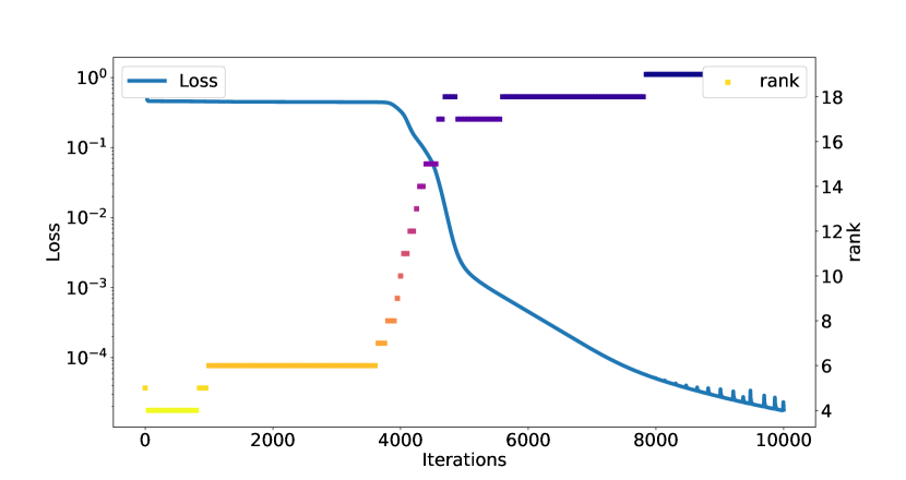
Figure 1: Staircase phenomenon of neuron functions in training dynamics.

As shown in the fig. 1, this increase in $\epsilon$-rank occurs in a stepwise fashion, closely resembling the structure of a staircase. Specifically, under standard parameter initialization, neuron functions initially exhibit low linear independence. Throughout the training process, variations in the loss function are closely linked to changes in the linear independence of these neuron functions. When the decline in the loss function reaches a plateau, the growth in linear independence tends to stabilize. Conversely, when the linear independence increases significantly, the loss experiences a rapid descent. We theoretically prove that the lower bound of the loss function decreases as the $\epsilon$-rank increases. This theoretical result holds for general deep neural networks. Consequently, achieving a sufficiently large $\epsilon$-rank is essential for ensuring a significant reduction in the loss function.

This naturally raises the question: how can a set of highly linearly independent neuron functions be learned efficiently? To address this, we identify several strategies from existing techniques that enable the neuron functions with a high $\epsilon$-rank at the early stage of training. Specifically, by designing appropriate initialization schemes and selecting well-suited network architectures, it is possible to ensure that the neuron functions exhibit high linear independence from the outset. Such approaches significantly accelerate the training process or improve the accuracy.

The main contributions of this work are summarized as follows:

• The introduction of effective rank provides a novel perspective for understanding the training dynamics of neural networks, revealing a staircase phenomenon. This phenomenon is observed universally across various tasks, including function fitting, handwriting recognition, and solving partial differential equations.

• We prove that the loss function of deep neural networks has a lower bound related to the $\epsilon$-rank. This bound decreases as the $\epsilon$-rank increases, thereby providing a theoretical explanation for the staircase phenomenon. Our analysis concludes that a sufficiently high $\epsilon$-rank is a necessary condition for achieving a significant reduction in the loss function.

• We investigate how $\epsilon$-rank evolves in existing advanced methodologies. Numerical examples show that these methodologies can construct neuron functions with a high $\epsilon$-rank rapidly, thereby significantly accelerating the training dynamics and improving model accuracy.

The rest of this paper is organized as follows. In section 2, the core concept of $\epsilon$-rank is defined through eigenvalues of the Gram matrix, and the staircase phenomenon is examined across various tasks and settings. A lower bound on the loss function with respect to the $\epsilon$-rank is given in section 3, which provides the theoretical explanation of the staircase phenomenon. The evolution of $\epsilon$-rank under existing methods is tested through numerical experiments in section 4, which include initialization methods, specific network structures and partial of unity technique in the random feature method. Concluding remarks are given in the last section.

2 Staircase Phenomenon

2.1 Preliminary

Before presenting the staircase phenomenon, we introduce several definitions that are extensions of linear algebra.

Definition 2.1.

The $n$ functions $f_{1}(x),\cdots,f_{n}(x)$ are linearly dependent in domain $\Omega$ if, there exists $c_{1},c_{2},\cdots,c_{n}\in\mathbb{R}$ not all zero s.t.

$$c_{1}f_{1}(x)+c_{2}f_{2}(x)+\cdots+c_{n}f_{n}(x)=0,\qquad\forall x\in\Omega.$$ (2)

If the functions are not linearly dependent, they are said to be linearly independent. For given $n$ functions $f_{1}(x),\cdots,f_{n}(x)$ in $L^{2}(\Omega)$, the mass matrix $M$ is defined as follows

$$(M)_{ij}:=\int_{\Omega}f_{i}(x)f_{j}(x)\mathrm{d}x,\quad 1\leq i,j\leq n.$$ (3)

Obviously $M$ is symmetric positive semi-definite.

Lemma 2.1.

$f_{1}(x),\cdots,f_{n}(x)$ in are linearly independent if and only if the rank of the mass matrix $r(M)=n$.

While the concept of linear dependence is well-defined in linear algebra, few functions in real-world applications strictly satisfy the condition specified in eq. 2. Consequently, a more practical and applicable indicator, extending beyond the framework of eq. 2, is required.

Definition 2.2.

The $n$ functions $f_{1}(x),\cdots,f_{n}(x)$ in are $\epsilon$-linearly dependent in domain $\Omega$ for some $\epsilon\geq 0$ if, there exists $c_{1},c_{2},\cdots,c_{n}\in\mathbb{R}$ with $\|\mathbf{c}\|^{2}=1$ s.t.,

$$\|c_{1}f_{1}+c_{2}f_{2}+\cdots+c_{n}f_{n}\|^{2}\leq\epsilon.$$ (4)

Otherwise they are said to be $\epsilon$-linearly independent.

Here $\|\cdot\|$ is the short note of $L^{2}$ norm, $\displaystyle\|u\|=\sqrt{\langle u,u\rangle}=\left(\int_{\Omega}u^{2}\mathrm{d}x\right)^{\frac{1}{2}}$. It is easy to check that $f_{1}(x),\cdots,f_{n}(x)$ are $\epsilon$-linearly independent if and only if the minimum eigenvalue of $M$ satisfies $\lambda_{\min}(M)>\epsilon.$ In the following, we intend to extend these concepts of linear independence to the neuron functions of a neural network.

Definition 2.3.

For a given neural network $u(x;\theta)$ defined on $\Omega\subset\mathbb{R}^{d}$ as

$$u(x;\theta)=\sum_{j=1}^{n}\beta_{j}\phi_{j}(x;\theta),$$

the Gram matrix $M_{u}$ is defined as below

$$(M_{u})_{ij}=\int_{\Omega}\phi_{i}(x;\theta)\phi_{j}(x;\theta)\mathrm{d}x.$$

Straightforwardly, we have the following definition of $\epsilon$-effective rank, $\epsilon$-rank for short.

Definition 2.4.

The $\epsilon$-rank of a neural network $u(x,\theta)$, associated with its Gram matrix $M_{u}$, is defined as

$$r_{\epsilon}(M_{u}):=|\{\lambda(M_{u})>\epsilon\}|,$$ (5)

where $|\cdot|$ denotes the cardinal number of a set.

The standard definitions of linear dependence and rank can be regarded as special cases corresponding to $\epsilon=0$. For simplicity, the linear independence and rank mentioned in experiments refer to $\epsilon$-linear independence and $\epsilon$-rank, respectively.

2.2 Staircase Phenomenon

With the necessary groundwork established, we now focus on how the $\epsilon$-rank of the neuron basis functions evolves throughout the training process of the neural network. Across various tasks, including function fitting, handwriting recognition, and solving partial differential equations, we consistently observe the following phenomenon.

Staircase phenomenon: In training dynamics, the loss function often decreases rapidly along with a significant growth of $\epsilon$-rank of neurons, and the evolution of the $\epsilon$-rank over time resembles a staircase-like pattern. The $\epsilon$-rank, as defined in definition 2.4, quantifies the linear independence or effective features of neuron functions in the last hidden layer. We experimentally demonstrate this phenomenon under different settings. To illustrate this phenomenon, we first consider a function fitting problem, which is one of the most fundamental tasks in neural networks.

Example 2.1 (Function fitting).

Consider the target function composed of multiple frequency components, defined as

$$f(x)=\cos x+\cos 2x+\cos 30x.$$ (6)

The computational domain is $\Omega=[-1,1]$, and the mean square error is used as the loss function.

This example consists of three distinct experimental settings:

• (fig. 2) Investigate the performance of neural networks with varying width and depth. The network configurations are as follows: (a) $L=2,n=50$. (b) $L=2,n=25$. (c) $L=4,n=50$. (d) $L=4,n=25$.

• (fig. 3) Analyze the $\epsilon$-rank of the neuron functions across different layers for a fixed network width of $n=50$ and depth of $L=4$.

• (fig. 4) Test neural networks with the following different activation functions:

  • ReLU: $\sigma(x)=\max(x,0)$.

  • ELU: $\sigma(x)=x,$ if $x>0$, and $\sigma(x)=\alpha(e^{x}-1)$, if $x<0$.

  • Cosine: $\sigma(x)=\cos(x)$.

  • Hyperbolic tangent: $\displaystyle\sigma(x)=\frac{e^{x}-e^{-x}}{e^{x}+e^{-x}}$

Under different width and depth, the training results are presented in fig. 2.

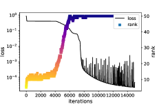
(a) b

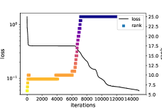
(b) b

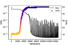
(c) b

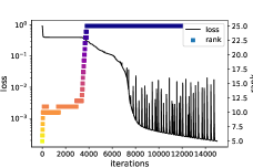
(d) b

Figure 2: (example 2.1) Staircase phenomenon under different width and depth. The black line is the mean square error and the gradient ladder is the $\epsilon$-rank.

The black line represents the loss function, while the scatters correspond to the $\epsilon$-rank of the mass matrix. When the linear independence of the neuron functions does not increase, the loss function stagnates for an extended period. However, once the neuron functions become fully linearly independent, the loss function rapidly decreases to a lower level, as shown in fig. 2(a), (c) and (d). Subfigure (b) demonstrates that shallow and narrow networks fail to approximate the target function efficiently under insufficient training. Another notable observation from fig. 2(d) is that, after attaining full rank, the loss function experiences a further sharp decline. This phase highlights a further unknown step in the learning process.

Additionally, we plot the $\epsilon$-rank of neurons in each hidden layer for the case of $L=4,n=50$ in fig. 3. The staircase phenomenon is observed in most hidden layers. The results also indicate that shallow neurons exhibit fewer features compared to deeper neurons. Within the same network, the $\epsilon$-rank of deeper neurons is consistently larger than that of shallow neurons. This observation suggests that deeper layers not only retain the linear independence of the preceding shallow layers but also further increase the complexity of the neuron functions, enabling the network to represent more intricate features. Notably, neurons in the first hidden layer fundamentally differ from that of deep layers. In the first layer, the neuron functions act as a set of basis functions that are directly formed by the activation function, without the composite transformation process that characterizes deeper networks.

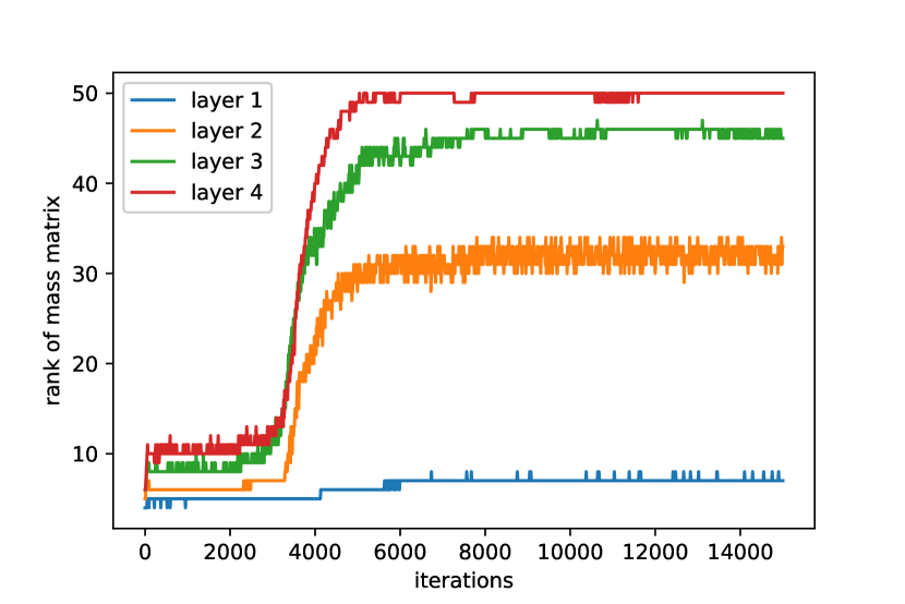
Figure 3: (example 2.1) The staircase phenomenon of different hidden layers in the same network

The appearance of staircase phenomenon is independent of the choice of activation function. fig. 4 illustrates the evolution of the $\epsilon$-rank during the training processes under several commonly used activation functions. The results show that while its behavior differs depending on the specific activation function used, staircase phenomenon is present across all activation functions. It can be observed that the upward trend and the peak value of the $\epsilon$-rank vary across different activation functions. This is because neural network function classes constructed with different activation functions exhibit distinct approximation capabilities with respect to the target function.

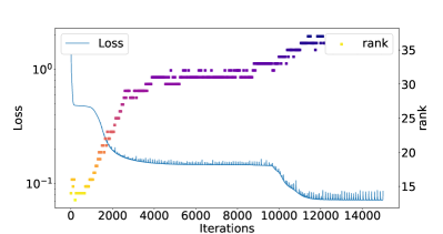
(a) ReLU

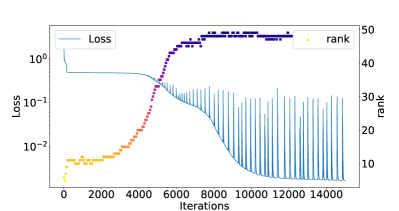
(b) ELU

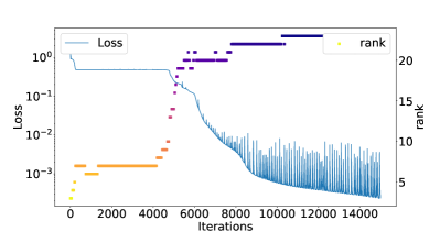
(c) Cosine

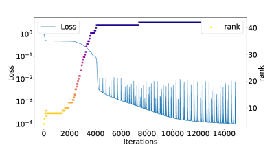
(d) Tanh

Figure 4: (example 2.1) Staircase phenomenon under different activation functions

Moreover, this phenomenon not only occurs in function fitting, but also in handwriting recognition and solving partial differential equations (section 4.1).

Example 2.2 (Handwriting recognition, fig. 5).

MNIST is a widely used database of handwritten digits for training various image processing systems. The dataset contains 70,000 grayscale images of handwritten digits (0 through 9), each with a resolution of 28x28 pixels. Thus, the dimension of the input is $d=784$. In this example, the cross entropy loss function is employed for training.

To address errors caused by high-dimensional numerical integration, we introduce an intermediate hidden layer with 10 neurons, using the neurons in this layer as sampling points for integration. As illustrated in fig. 5, the staircase phenomenon is evident in the handwriting recognition task, demonstrating that this phenomenon can also be observed in high-dimensional problems. This observation underscores the representational power of neural networks, which can effectively construct high-dimensional feature spaces, that is notably challenging in traditional scientific computing.

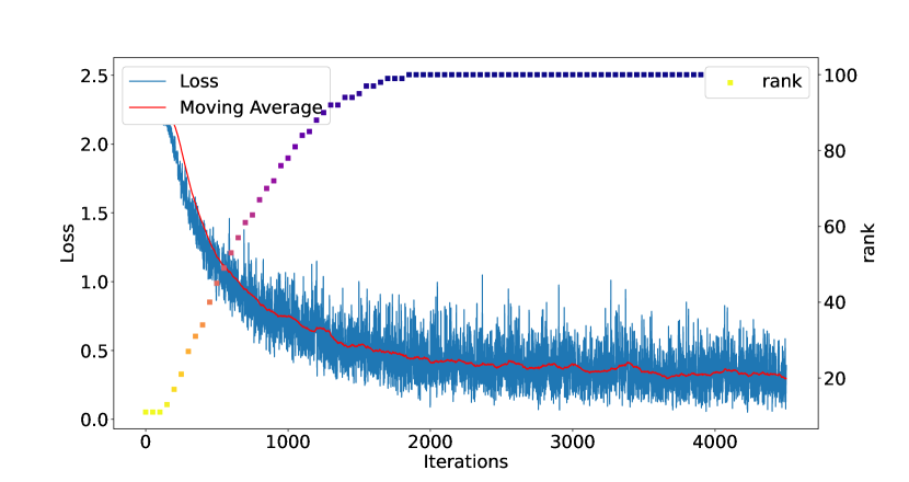
Figure 5: (example 2.2) Ladders phenomenon in handwriting recognition.

To gain a clearer understanding of the training mechanism, it is necessary to investigate why the staircase phenomenon occurs. Many widely used initialization methods do not ensure that the neuron functions are fully linearly independent after initialization. Therefore, the first stage of training involves separating the neuron functions post-initialization. This is when the staircase phenomenon typically occurs.

Existing widely used initialization methods, like Xavier or Glorot initialization method [9], initialize the weights and biases as $\displaystyle w_{j},b_{j}\sim U(-\frac{1}{\sqrt{n}},\frac{1}{\sqrt{n}})$. Consider a simple neuron function $\phi(x)=\sigma(wx+b),\ x\in[-1,1],$ with the hyperbolic tangent activation function $\sigma(x)=\tanh(x)$. Since $\sigma^{\prime}(0)=1$, the activation function behaves approximately as a linear function near zero:

$$\phi(x)=wx+b-\frac{(wx+b)^{3}}{3}+o((w+b)^{3})\sim wx+b.$$

As the linear combination of linear functions is also linear, the $\epsilon$-rank of $\displaystyle\{\phi_{i}\}_{i=1}^{n}$ after initialization is approximately two.

This explains why, during the training process of function fitting, neural networks often experience a plateau in the loss function that takes time to overcome. Initially, this plateau arises because the initialized basis functions are not fully linearly independent. This phase can be interpreted as feature extraction. From our perspective, at specific stages during training, this process requires the separation of neuron functions and an increase in their $\epsilon$-rank.

3 Theoretical Explanation of the Staircase Phenomenon

In this section, we demonstrate the theoretical significance of $\epsilon$-rank and provide an explanation of the staircase phenomenon. For well-posed problems, when the solution lies outside the class of neural network functions, we demonstrate that an increase in $\epsilon$-rank during the training process is a necessary condition for a reduction in the loss function.

It is trivial that if $f$ is a linear combination of $f_{1},f_{2},\cdots,f_{n}$ with $r(M)=p$, then $f$ can be rewritten as a linear combination of $p$ of them. Similarly, if $r_{\epsilon}(M)=p$, a comparable result holds. We begins with the following useful lemma constructed in [14].

Lemma 3.1.

[14] Let $Q\in\mathcal{O}_{n,p}$ with $p\leq n$, and $\{Q_{1},Q_{2},\cdots,Q_{k}\}$ is the set of all $p$-by-$p$ sub-matrices of $Q$ where $k=\begin{pmatrix}n\\ p\end{pmatrix}$. Define a vector in $\mathbb{R}^{k}$ by $\sigma(Q)=\left(\sigma_{\min}\left(Q_{1}\right),\sigma_{\min}\left(Q_{2}\right),\cdots,\sigma_{\min}\left(Q_{k}\right)\right)^{T}$. Then

$$\inf_{Q\in\mathcal{O}_{n,p}}\left(\|\sigma\left(Q\right)\|_{\infty}\right)\geq\frac{1}{\sqrt{p(n-p)+\min(p,n-p)}}.$$

Theorem 3.1.

If $\displaystyle f=\sum_{j=1}^{n}\beta_{j}f_{j}$ with $\|\mathbf{\beta}\|^{2}\leq C$, $r_{\epsilon}(M_{f})=p$ for some $\epsilon\geq 0$ and positive integer $p\leq n$, then after a reorder of set $\{f_{1},\cdots,f_{n}\}=\{\tilde{f_{1}},\cdots,\tilde{f_{n}}\}$ if necessary, $f$ can be approximated by $\displaystyle\tilde{f}=\sum_{j=1}^{p}\tilde{\beta_{j}}\tilde{f_{j}}$ with $\|f-\tilde{f}\|^{2}\leq C(p+1)(n-p)^{2}\epsilon$.

Proof.

Consider the spectral decomposition $M=Q\Lambda Q^{T}$, $Q$ is orthogonal, $\Lambda=\text{diag}([\lambda_{1},\lambda_{2},\cdots,\lambda_{n}])$ is diagonal with eigenvalues $\lambda_{1}\geq\cdots\geq\lambda_{p}>\epsilon\geq\lambda_{p+1}\geq\cdots\geq\lambda_{n}\geq 0$. For simplicity, we denote $\beta=\begin{bmatrix}\beta_{1}&\cdots&\beta_{n}\end{bmatrix}^{T}$ and $F=\begin{bmatrix}f_{1}&\cdots&f_{n}\end{bmatrix}^{T}$, thus $f=\beta^{T}F$. Let $P$ be a permutation matrix, and denote

$$PQ=\left[\begin{array}[]{cc}V_{11}&V_{12}\\ V_{21}&V_{22}\end{array}\right]\begin{array}[]{l}\scriptstyle p\\ \scriptstyle n-p\end{array}\vskip-10.00002pt$$

$$\begin{array}[]{cc}\scriptstyle p&\hskip 5.0pt\scriptstyle n-p\end{array}$$

as a partitioning of the matrix $PQ$. Now we construct an approximation of $f$ by $\tilde{f}=\tilde{\beta}^{T}\tilde{F}$, where

$$\tilde{\beta} =\begin{bmatrix}I_{p}&0\end{bmatrix}P\beta-V_{12}V_{22}^{-1}\begin{bmatrix}0&I_{n-p}\end{bmatrix}P\beta,$$

$$\tilde{F} =\begin{bmatrix}I_{p}&0\end{bmatrix}PF.$$

To estimate $L_{2}$ error of $\|f-\tilde{f}\|^{2}$, we note that

$$\quad\,\,\|f-\tilde{f}\|^{2}$$

$$=\|(P\beta)^{T}(PF)-\left(\begin{bmatrix}I_{p}&0\end{bmatrix}P\beta-V_{12}V_{22}^{-1}\begin{bmatrix}0&I_{n-p}\end{bmatrix}P\beta\right)^{T}\begin{bmatrix}I_{p}&0\end{bmatrix}PF\|^{2}$$

$$=\|\left(\begin{bmatrix}0&I_{n-p}\end{bmatrix}P\beta\right)^{T}\left(\begin{bmatrix}0&I_{n-p}\end{bmatrix}PF\right)+\left(\begin{bmatrix}0&I_{n-p}\end{bmatrix}P\beta\right)^{T}V_{22}^{-T}V_{12}^{T}\begin{bmatrix}I_{p}&0\end{bmatrix}PF\|^{2}$$

$$=\|\left(\begin{bmatrix}0&I_{n-p}\end{bmatrix}P\beta\right)^{T}V_{22}^{-T}\left(V_{22}^{T}\begin{bmatrix}0&I_{n-p}\end{bmatrix}PF+V_{12}^{T}\begin{bmatrix}I_{p}&0\end{bmatrix}PF\right)\|^{2}$$

$$=\|\left(\begin{bmatrix}0&I_{n-p}\end{bmatrix}P\beta\right)^{T}V_{22}^{-T}\left(PQ\begin{bmatrix}0&I_{n-p}\end{bmatrix}^{T}\right)^{T}PF\|^{2}$$

$$=\|\left(\begin{bmatrix}0&I_{n-p}\end{bmatrix}P\beta\right)^{T}V_{22}^{-T}\begin{bmatrix}0&I_{n-p}\end{bmatrix}Q^{T}F\|^{2}$$

$$\leq\|\beta\|^{2}\|V_{22}^{-T}\|^{2}\left(\lambda_{p+1}+\cdots+\lambda_{n}\right)$$

$$\leq C\|V_{22}^{-T}\|^{2}(n-p)\epsilon.$$

It remains to control the term $\|V_{22}^{-T}\|^{2}$. By lemma 3.1, for any orthogonal matrix $Q$, there exists a permutation $P$, such that $\|V_{22}^{-T}\|^{2}\leq(p+1)(n-p)$. ∎

It is worth noting that the bound established in the theorem is quite loose. The final inequality in the proof straightforwardly bounds $\lambda_{p+1}+\cdots+\lambda_{n}$ by $(n-p)\epsilon$ despite the potential for rapid decay of the eigenvalues in practice. Moreover, the bound in lemma 3.1 is not sharp, except for $p=1$ and $p=n-1$. We conjecture that $\frac{1}{\sqrt{n}}$ provides the sharp bound for all $p$, supported by extensive numerical experiments that have yet to produced a counterexample.

We then apply the theorem to the neural networks. The $L$-layer neural network is represented as follows:

$$\mathcal{F}_{n} =\left\{\sum_{i=1}^{n}\beta_{j}\phi_{j}(x;\theta)\bigg{|}\phi_{j}(x;\theta)\in\mathcal{H}_{L},\beta_{j}\in\mathbb{R},j=1,\cdots,n\right\},$$ (7)

$$\mathcal{H}_{k} =\left\{\sigma(w_{k}\cdot y(x)+b_{k})\bigg{|}y(x)\in\mathbb{R}^{n_{k-1}},y_{j}(x)\in\mathcal{H}_{k-1},\right.$$

$$\qquad\left.w_{k}\in\mathbb{R}^{n_{k-1}},b_{k}\in\mathbb{R}\vphantom{\bigg{|}}\right\},\quad k=1,\cdots,L,$$

$$\mathcal{H}_{0} =\left\{x\in\Omega\subset\mathbb{R}^{d}\right\}.$$

where $\{\beta_{j}\}_{j=1}^{n}$ and $\displaystyle\theta=\{(W_{k},B_{k})\}_{k=1}^{L}$ are trainable coefficients, and $\sigma$ is the activation function satisfying the universal approximation theorem of neural networks [15]. The two-layer (shallow) neural network is a special case when $L=1$.

Consider the following loss function:

$$\min_{u\in\mathcal{F}_{n}}\mathcal{L}(u)=\|\mathcal{G}(u)-f\|^{2},$$ (8)

where $f\in L^{2}(\Omega)$ represents the target function or data. If the exact solution $u^{*}$ does not belong to the function class $\mathcal{F}_{n}$, it follows that the neuron functions of the optimizer $u_{n}^{*}\in\mathcal{F}_{n}$ are linearly independent, that is, $r(M_{u_{n}^{*}})=n$. Equivalently, for a wider network, we can always find a better approximator, that is,

$$\text{dist}(u^{*},\mathcal{F}_{n})<\text{dist}(u^{*},\mathcal{F}_{m}),\quad m<n,$$

where $\text{dist}(u,A)=\min_{v\in A}\|u-v\|$.

However, as previously mentioned, the neuron functions are almost surely linearly independent with probability close to 1. The following theorem highlights the importance of the $\epsilon$-rank during the training process.

Theorem 3.2.

Given the problem $\mathcal{G}(u)=f$ and $\mathcal{G}^{-1}$ being the solution operator, assume that the problem satisfies the following stability condition, for any $u,v$,

$$\|\mathcal{G}^{-1}(u)-\mathcal{G}^{-1}(v)\|\leq C_{S}\|u-v\|.$$ (9)

Let $u_{n}$ be an arbitrary approximation in $\mathcal{F}_{n}$ with the $\epsilon$-rank equalling to $p$, i.e.,

$$u_{n}(x;\theta)=\sum_{j=1}^{n}\beta_{j}\phi_{j}(x;\theta),$$

where $\|\beta\|^{2}\leq C$ and $r_{\epsilon}(M_{u_{n}})=p$. Then

$$\sqrt{\mathcal{L}(u_{n})}\geq\frac{1}{C_{s}}\left(dist(u^{*},\mathcal{F}_{p})-\sqrt{C(p+1)(n-p)^{2}\epsilon}\right),$$ (10)

where $u^{*}=\mathcal{G}^{-1}(f)$ is the exact solution, $\mathcal{L}(u)=\|\mathcal{G}(u)-f\|^{2}$ is the loss function.

Proof.

By theorem 3.1, there exists a $u_{p}\in\mathcal{F}_{p}$ satisfying $\|u_{p}-u_{n}\|^{2}\leq C(p+1)(n-p)^{2}\epsilon$. A triangular inequality

$$\text{dist}(u^{*},\mathcal{F}_{p}) \leq\|u^{*}-u_{p}\|$$

$$\leq\|u_{p}-u_{n}\|+\|u_{n}-u^{*}\|$$

$$\leq\sqrt{C(p+1)(n-p)^{2}\epsilon}+\|u_{n}-u^{*}\|$$

$$=\sqrt{C(p+1)(n-p)^{2}\epsilon}+\|\mathcal{G}^{-1}(\mathcal{G}(u_{n}))-\mathcal{G}^{-1}(f)\|$$

$$\leq\sqrt{C(p+1)(n-p)^{2}\epsilon}+C_{S}\|\mathcal{G}(u_{n})-f\|$$

gives the desired inequality. ∎

Remark 3.1.

The stability assumption (9) is reasonable for well-posed problems. For instance, in the function fitting problems, $\mathcal{G}=\mathcal{I}$, $C_{S}=1$, and the loss function is $\mathcal{L}(u)=\|u-f\|^{2}$. In the case using PINN to solve Poisson equation $-\Delta u=f$, $C_{S}=\|(-\Delta)^{-1}\|$ is uniformly bounded.

Remark 3.2.

When the $\epsilon$-rank of the neural network approximator $u_{n}\in\mathcal{F}_{n}$ is $r_{\epsilon}\left(M_{u_{n}}\right)=p$, the result of the theorem can be expressed as

$$\sqrt{\mathcal{L}(u_{n})}\geq\frac{\text{dist}(u^{*},\mathcal{F}_{p})}{C_{S}}-O(\sqrt{\epsilon}).$$

Recall that $\epsilon$ is a fixed hyperparameter, and it is chosen sufficiently small, which yields the loss function has a lower bound in terms of $\text{dist}(u^{*},\mathcal{F}_{p})$. During the training process, to minimize the loss function $\mathcal{L}(u)$, there must be a decrease in $\text{dist}(u^{*},\mathcal{F}_{p})$, implying an increase in the $\epsilon$-rank of the neuron functions.

Remark 3.3.

If $\epsilon$ is sufficiently small and the loss function is minimized to an optimal level while $p$ remains small relative to $n$, then theorem 3.2 offers an alternative explanation: $p$ neurons can approximate the solution well, and more features are unnecessary. This is one of the reasons why neurons pruning [37, 25] is feasible in computation.

4 $\epsilon$-rank in Existing Methods

This section presents how the $\epsilon$-rank evolves in various existing methodologies. A considerable number of methods facilitate the linear independence of neuron functions during the initial stages of the training process. These approaches have been demonstrated to accelerate of the training process and enhance the accuracy of the resulting models. Based on this, it is beneficial to ensure that the neuron functions exhibit a relatively high $\epsilon$-rank at the outset.

The neural network structure is defined as eq. 1. Unless otherwise mentioned, the activation function is hyperbolic tangent function $\sigma(x)=\tanh(x)$. $L^{2}$ norm is used to measure errors between predicted solution $u$ and exact solution or reference solution $u^{*}$.

$$e=\|u-u^{*}\|,\qquad\tilde{e}=\frac{\|u-u^{*}\|}{\|u^{*}\|},$$

where $\displaystyle\|u\|=\left(\int_{\Omega}u^{2}\mathrm{d}x\right)^{\frac{1}{2}}$ is the short note of $L^{2}$ norm.

In numerical calculations, we extend the $\epsilon$-linear independence to the discrete form. Given $n$ functions discretized on $m$ nodes

$$D=\begin{pmatrix}\phi_{1}(x_{1})&\cdots&\phi_{n}(x_{1})\\ \phi_{1}(x_{2})&\cdots&\phi_{n}(x_{2})\\ \vdots&\ddots&\vdots\\ \phi_{1}(x_{m})&\cdots&\phi_{n}(x_{m})\end{pmatrix},$$

the mass matrix is computed by $M=D^{T}WD$, where $W$ is the weight matrix. The $\epsilon$-linear independence of these $n$ functions is

$$r_{\epsilon}(M)=|A|,\quad A=\{|\lambda(M)|>\epsilon\},$$

where $|A|$ is the cardinal number of $A$, and the tolerance is given $\epsilon=10^{-6}$.

The rank of mass matrix, $r_{\epsilon}(M)$ is employed to measure the linear independence of the basis functions.

In low-dimensional cases, $M$ is approximated using numerical integration, while in high dimensions, $M$ is approximated by Monte Carlo integration. For simplicity, we generate one set of integration data points $\{x\}_{k=1}^{m}$, which can be Gaussian integral points or uniform mesh for $d=1,2$. Then

$$(M)_{ij}\approx\sum_{k=1}^{m}w_{k}\phi_{i}(x_{k})\phi_{j}(x_{k}),$$ (11)

where $w_{k}$ are the integral weights. For example, $w_{0}=w_{m}=\frac{1}{2}$ and $w_{i}=1,i=2,\cdots,m-1$ is the trapezoidal formulation.

The notations are listed in table 1.

Table 1: The List of Notations

Notation	Stands for …
$L$	Depth of hidden layers
$n$	Width of hidden layers
$N$	Number of total parameters
$m$	Sample size
$d$	Dimension of the input
$\phi$	The neurons of the output layer
$\beta$	Coefficients of the output layer
$M(\phi)$	The mass matrix of basis functions $\{\phi_{j}\}_{j=1}^{n}$
$r_{\epsilon}(M)$	The $\epsilon$-rank of the mass matrix
$\epsilon$	Tolerance of eigenvalues

4.1 Deterministic Initialization

This subsection evaluates the feasibility of directly constructing highly linearly independent neuron functions through initialization.

Example 4.1 (function fitting with initialization, fig. 6).

In this example, we consider a function fitting problem where the target function is also defined as eq. 6

$$u(x)=\cos(x)+\cos(2x)+\cos(30x),\qquad x\in[-1,1].$$

We compare two initialization methods: deterministic and random initialization. For the deterministic initialization, the first layer of the neural network is initialized as:

$$y_{1}=\sigma(w_{0}x+b_{0}),$$ (12)

where the weights and biases are given by $\displaystyle(w_{0})_{j}=\frac{n}{2},\ (b_{0})_{j}=\frac{n}{2}-j,\ j=1,\cdots,n$.

As discussed in section 2, a set of linearly independent neuron functions is important for neural network performance. A straightforward method to improve the $\epsilon$-rank of neurons is to expand the range of the uniform distribution. For example, set $\theta\sim U(-m,m)$. While this approach can enhance the linear independence of the neuron basis functions, it is not commonly used in practice due to the potential issues it introduces. As mentioned in [9], such an initialization strategy can lead to problems like exploding gradients and the saturation of activation functions, which negatively affect the training process.

Inspired by traditional numerical methods, we propose an alternative initialization method for the first layer of the neural network when $d=1$, which guarantees a sufficiently high $\epsilon$-rank of neuron functions. Specifically, the initialization for the first hidden layer is given as eq. 12, which can be rewritten in the form of

$$(y_{1})_{j}=\tanh(\frac{n}{2}(x-x_{j})),\quad j=1,\cdots,n,$$ (13)

where $\{x_{j}\}$ are the uniform grids on $[-1,1]$.

The result is shown in fig. 6. This figure clearly illustrates that once the neuron functions exhibit sufficient linear independence, the loss function will be rapidly optimized. Comparing the blue curve (loss = $10^{-5}$) in fig. 6(a) and the orange curve (loss = $10^{-4}$) in fig. 6(b), even a shallow and narrow network performs better than a deeper and wider network. This indicates that a good initialization method can greatly reduce training time and improve training accuracy.

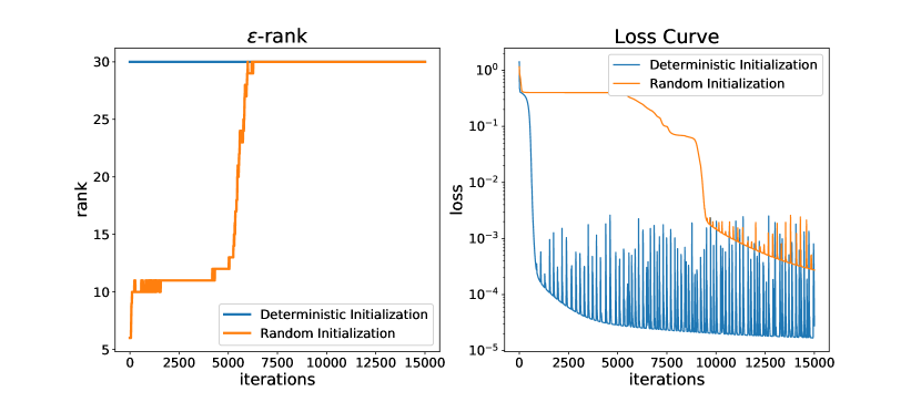
(a) $L=2,n=30$

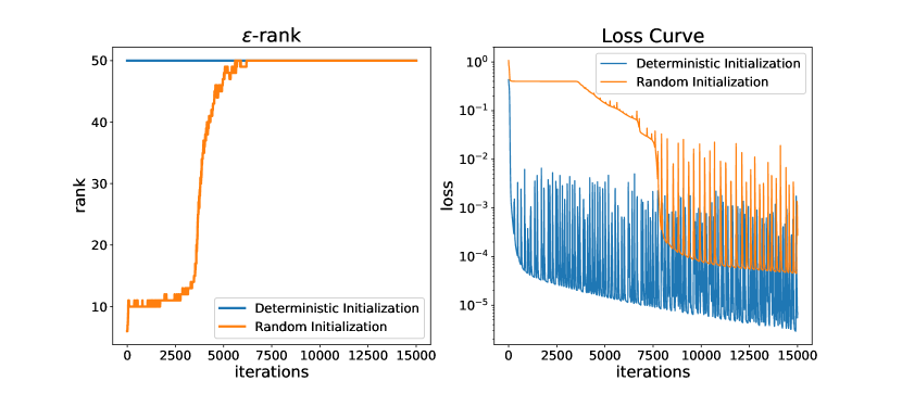
(b) $L=4,n=50$

Figure 6: (example 4.1) The training process of neural networks with default settings and deterministic initialization. The left figure shows the linear independence and the right figure plots the losses. The blue curve gives the result of deterministic initialization method and the orange curve is under default settings.

We now demonstrate that the staircase phenomenon also arises when solving partial differential equations and that appropriate initialization techniques can significantly enhance performance. Since the work of [29], physics-informed neural networks (PINN) have achieved remarkable success in the field of computational science. Numerous studies have highlighted the advantages of neural network based algorithms for partial differential equations in high dimensional problems [31, 8, 7], irregular domains [38, 33] and systems with complex mechanisms [22, 20].

Consider the following boundary value problem:

Example 4.2 (Solving Possion’s equation by PINN, fig. 7).

$$\left\{\begin{aligned} -\Delta u&=f,&&x\in\Omega,\\ u&=0,&&x\in\partial\Omega,\end{aligned}\right.$$

where $\displaystyle\Omega=\left[-\frac{\pi}{2},\frac{\pi}{2}\right]^{2},\ f(x,y)=8\sin 2x\sin 2y$. The analytic solution of this differential equation is $u(x,y)=\sin 2x\sin 2y$. The loss function is defined as

$$\mathcal{L}(u)=\|\Delta u+f\|_{L^{2}(\Omega)}^{2}+\|u\|_{L^{2}(\partial\Omega)}^{2}.$$ (14)

The previously used initialization method becomes ineffective in this context, as the problem is two-dimensional. In [41], the authors proposed a method for generating uniformly distributed neurons in shallow networks to ensure equal expressive power across all regions of the domain. Inspired by this approach, we can separate the neuron functions in the first hidden layer by employing a uniformly distributed initialization method. This method re-parameterizes the weight and bias of each neuron in the first hidden layer as:

$$\sigma(w_{j}^{T}x+(b_{0})_{j})=\sigma(\gamma_{j}(a_{j}^{T}x+r_{j})),$$ (15)

where $w_{j}^{T}$ is the j-th rows of $W_{0}$, $\|a_{j}\|^{2}=1$, and $\gamma_{j}\geq 0$. $\{a_{j}\}_{j=1}^{n}$ are initialized by uniformly sampled on the unit sphere, and $\{r_{j}\}_{j=1}^{n}$ are initialized by uniformly sampled on a bounded positive real line related to $\Omega$. This initialization method generate neurons with uniform hyperplane density in the region, termed as uniform density initialization (UDI).

The result is presented in fig. 7, which clearly demonstrate that solving PDEs with neural networks also exhibits the staircase phenomenon. Furthermore, the figure highlights that an effective initialization technique, which ensures a high $\epsilon$-rank, can significantly accelerate the training process.

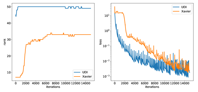
Figure 7: (example 4.2) The training process of solving 2-D Poisson’s equation with default Xavier initialization and uniformly density initialization (UDI). The left figure shows the $\epsilon$-rank and the right figure shows losses. The blue curve gives the result of uniformly density initialization and the red curve is under Xavier initialization.

4.2 Partial of Unity

Next, we evaluate the $\epsilon$-rank in two methods that do not involve training process. Both extreme learning machine (ELM) [17] and random features [28] are widely used techniques in deep learning. Notably, neither method involves training the hidden layers, offering computationally efficient solutions. In these approaches, the linear independence of the neuron functions depends solely on the initialization and network structure employed.

An important improvement is the partition of unity method (PoU) technique, employed in the random feature method (RFM) [2] and local extreme learning machine [6]. In RFM, the approximate solution is expressed as a linear combination of random features combined with the PoU, as follows:

$$u_{R}(x)=\sum_{i=1}^{m}\psi_{i}(x)\sum_{j=1}^{J_{R}}u_{ij}\phi_{ij}(x),$$

where $u_{ij}$ are unknown coefficients. In RFM, $N$ points $\{x_{i}\}_{i=1}^{N}$ are chosen from $\Omega$, typically uniformly distributed. Then $\Omega$ is decomposed to $N$ disjoint subdomains $\{\Omega_{i}\}_{i=1}^{N}$ with $x_{i}\in\Omega_{i}$. For each $\Omega_{i}$, a PoU function $\psi_{i}$ is constructed with support $\Omega_{i}$, i.e., $\text{supp}(\psi_{i})=\Omega_{i}$. The commonly used PoU function is

$$\psi_{i}(x)=\mathbb{I}_{\Omega_{i}}(x).$$

Since $|\Omega_{i}\cap\Omega_{j}|=0$, it is clear that $\displaystyle\{\psi_{i}\sum_{j=1}^{J_{R}}u_{ij}\phi_{ij}\}_{i=1}^{N}$ are $\epsilon$-linearly independent when $\|\psi_{i}\sum_{j=1}^{J_{R}}u_{ij}\phi_{ij}\|^{2}>\epsilon$. The extreme learning machine is modeled as

$$u_{E}(x)=\sum_{j=1}^{J_{E}}u_{j}\phi_{j}(x),$$

which can be seen as a random feature method with no subdomains ($N=1$).

Example 4.3 (Two dimensional function fitting, fig. 8).

$$u^{*}(x,y)=\cos x\cos y+\cos 10x\cos 10y,\quad\Omega=[-1,1]^{2}.$$

In this example, we compare the performance of modeling with and without the partition of unity (PoU) technique, regarded as the RFM and ELM respectively. The number of neurons is set to $n=900$. In the RFM, these $900$ neurons are divided into $3\times 3$ sub-intervals, i.e., $i=9,J_{R}=100$ and in the ELM, $J_{E}=900$. The coefficients of the output layer in both methods are determined using the least squares method.

The results, presented in fig. 8, demonstrate that, for the same number of neurons, the RFM achieves greater linear independence due to the compact support in each subdomain, resulting in higher accuracy. This example clearly illustrates that, under identical configurations, achieving a high linear independence through specific techniques can significantly enhance network performance. Furthermore, an approximate inverse proportional relationship between the $\epsilon$-rank and the error is observed.

(a) solution of ELM

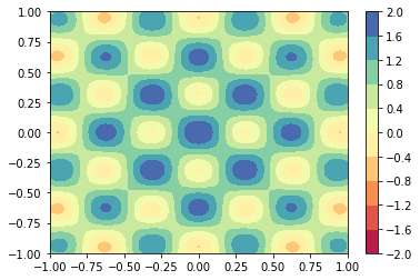
(b) solution of RFM

(c) exact solution

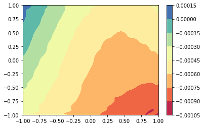
(d) error of ELM

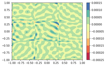
(e) error of RFM

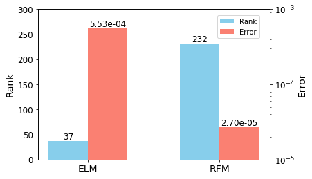
(f) rank and error

Figure 8: (example 4.3) (a)-(e) are the solutions and point-wise errors of random feature method and extreme learning machine method. The last subfigure (f) shows the rank and $L^{2}$ error of two methods.

4.3 ResNet

The network structure has a significant impact on the linear independence of neuron functions. The Residual Network (ResNet), is a deep neural network architecture introduced by [12]. ResNet has been widely adopted in the field of deep learning, particularly for the training of very deep networks.

The typical structure of the ResNet is the residual block, which is given as

$$y=R(x)=x+\sigma(W_{1}\sigma(W_{2}x+b_{2})+b_{1}).$$

The shortcut connection allows the input of the block to bypass the transformations and connect directly to its output. This shortcut provides a direct path for the gradient, facilitating more effective backpropagation and addressing the degradation problem, where deeper networks may perform worse than their shallower counterparts.

When the neuron functions in deeper layers are connected to the neuron functions in shallower layers via a residual block, i.e.,

$$\phi^{L+1}(x)=R(\phi^{L}(x)),$$

this architecture demonstrates an additional advantage: it helps sustain the growth of the $\epsilon$-rank.

Example 4.4 (Function fitting with ResNet, figs. 9 and 10).

This example examines the $\epsilon$-rank in each layer of the ResNet compared to MLP. To ensure a comparable number of parameters and to make each layer of neuron functions observable, we employ a one-layer residual block. The ResNet structure is defined as follows:

$$\left\{\begin{aligned} y_{0}&=x,\\ y_{k+1}&=y_{k}+\sigma(W_{k}y_{k}+b_{k}),&k=0,\cdots,L-1,\\ y&=\beta\cdot y_{L}.\end{aligned}\right.$$ (16)

The problem is the same function fitting problem as example 2.1.

In fig. 9, we observe that the $\epsilon$-rank of ResNet is initially higher and grows faster to full rank compared to the MLP. Furthermore, as shown in fig. 10, the residual block structure ensures greater rank growth in the deeper neuron functions.

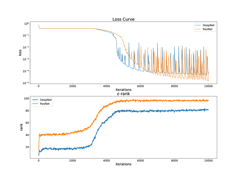
Figure 9: (example 4.4) The training result between ResNet and fully connected neural network.

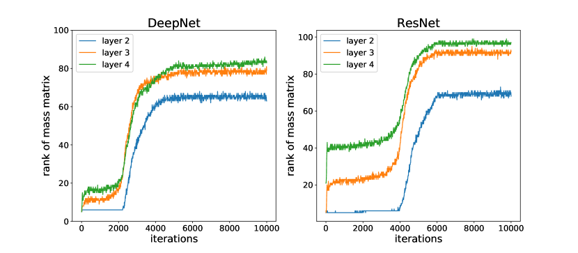
Figure 10: (example 4.4) The $\epsilon$-rank for each layer of neuron functions in DeepNet and ResNet.

This example demonstrates that the linear independence of neuron functions varies across different network structures. Selecting a network architecture that promotes linear independence among neuron functions enables the capture of more features, thereby improving performance.

5 Concluding Remarks

In summary, this research provides a novel perspective on the training dynamics of deep neural networks by drawing connections to traditional numerical analysis. A key finding of our study is the identification of the staircase phenomenon, which describes a stepwise increase in the linear independence of neuron functions during the training process, typically associated with rapid decreases in the loss function. This finding highlights the importance of establishing a diverse and robust set of neuron functions in the early stages of training, which promotes both efficiency and convergence in model optimization.

Theoretical analyses and numerical experiments confirm that a set of linearly independent basis neuron functions is essential for effectively minimizing the loss function of neural networks. The training process can be significantly accelerated by leveraging appropriate techniques, such as deterministic initialization methods, constructing efficient network architectures, and employing proper domain partitioning. These strategies have shown effective in promoting the linear independence of neuron functions, providing insight into the success of certain neural network approaches.

This study offers a deeper understanding of the mechanisms underlying deep learning by bridging neural network framework with traditional numerical methods. It provides a solid foundation for future innovations in network initialization, training methodologies, and the design of more efficient models.

References

- [1] A. Bietti and J. Mairal, On the Inductive Bias of Neural Tangent Kernels, in Advances in Neural Information Processing Systems, vol. 32, Curran Associates, Inc., 2019, pp. 12893–12904.
- [2] J. Chen, W. E, and Y. Luo, The Random Feature Method for Time-Dependent Problems, East Asian Journal on Applied Mathematics, 13 (2023), pp. 435–463.
- [3] J. Chen, W. E, and Y. Sun, Optimization of Random Feature Method in the High-Precision Regime, Communications on Applied Mathematics and Computation, 6 (2024), pp. 1490–1517.
- [4] Z. Chen, Y. Cao, Q. Gu, and T. Zhang, A Generalized Neural Tangent Kernel Analysis for Two-layer Neural Networks, in Advances in Neural Information Processing Systems, vol. 33, Curran Associates, Inc., 2020, pp. 13363–13373.
- [5] L. Dinh, R. Pascanu, S. Bengio, and Y. Bengio, Sharp Minima Can Generalize For Deep Nets, in Proceedings of the 34th International Conference on Machine Learning, PMLR, July 2017, pp. 1019–1028.
- [6] S. Dong and Z. Li, Local extreme learning machines and domain decomposition for solving linear and nonlinear partial differential equations, Computer Methods in Applied Mechanics and Engineering, 387 (2021), p. 114129.
- [7] W. E, J. Han, and A. Jentzen, Deep learning-based numerical methods for high-dimensional parabolic partial differential equations and backward stochastic differential equations, Communications in Mathematics and Statistics, 5 (2017), pp. 349–380.
- [8] W. E and B. Yu, The deep Ritz method: A deep learning-based numerical algorithm for solving variational problems, Communications in Mathematics and Statistics, 6 (2018), pp. 1–12.
- [9] X. Glorot and Y. Bengio, Understanding the difficulty of training deep feedforward neural networks, in Proceedings of the Thirteenth International Conference on Artificial Intelligence and Statistics, 2010, pp. 249–256.
- [10] J. He, L. Li, and J. Xu, ReLU deep neural networks from the hierarchical basis perspective, Computers & Mathematics with Applications, 120 (2022), pp. 105–114.
- [11] J. He, L. Li, J. Xu, and C. Zheng, Relu Deep Neural Networks and Linear Finite Elements, Journal of Computational Mathematics, 38 (2020), pp. 502–527.
- [12] K. He, X. Zhang, S. Ren, and J. Sun, Deep residual learning for image recognition, in Proceedings of the IEEE Conference on Computer Vision and Pattern Recognition, 2016, pp. 770–778.
- [13] S. Hochreiter and J. Schmidhuber, Flat Minima, Neural Computation, 9 (1997), pp. 1–42.
- [14] Y. P. Hong and C.-T. Pan, Rank-revealing factorizations and the singular value decomposition, Mathematics of Computation, 58 (1992), pp. 213–232.
- [15] K. Hornik, Approximation capabilities of multilayer feedforward networks, Neural Networks, 4 (1991), pp. 251–257.
- [16] G.-B. Huang, L. Chen, and C.-K. Siew, Universal Approximation using Incremental Constructive Feedforward Networks with Random Hidden Nodes, IEEE Transactions on Neural Networks, 17 (2006), pp. 879–892.
- [17] G.-B. Huang, Q.-Y. Zhu, and C.-K. Siew, Extreme learning machine: Theory and applications, Neurocomputing, 70 (2006), pp. 489–501.
- [18] A. Jacot, F. Gabriel, and C. Hongler, Neural Tangent Kernel: Convergence and Generalization in Neural Networks, in Advances in Neural Information Processing Systems, vol. 31, Curran Associates, Inc., 2018, pp. 8580–8589.
- [19] N. S. Keskar, D. Mudigere, J. Nocedal, M. Smelyanskiy, and P. T. P. Tang, On large-batch training for deep learning: Generalization gap and sharp minima, in International Conference on Learning Representations, 2017.
- [20] C. L. Wight and J. Zhao, Solving Allen-Cahn and Cahn-Hilliard Equations Using the Adaptive Physics Informed Neural Networks, Communications in Computational Physics, 29 (2021), pp. 930–954.
- [21] H. Li, Z. Xu, G. Taylor, C. Studer, and T. Goldstein, Visualizing the Loss Landscape of Neural Nets, in Advances in Neural Information Processing Systems, vol. 31, Curran Associates, Inc., 2018, pp. 6391–6401.
- [22] Z. Liu, W. Cai, and Z.-Q. John Xu, Multi-Scale Deep Neural Network (MscaleDNN) for Solving Poisson-Boltzmann Equation in Complex Domains, Communications in Computational Physics, 28 (2020), pp. 1970–2001.
- [23] R. E. Meethal, A. Kodakkal, M. Khalil, A. Ghantasala, B. Obst, K.-U. Bletzinger, and R. Wüchner, Finite element method-enhanced neural network for forward and inverse problems, Advanced Modeling and Simulation in Engineering Sciences, 10 (2023), p. 6.
- [24] S. K. Mitusch, S. W. Funke, and M. Kuchta, Hybrid FEM-NN models: Combining artificial neural networks with the finite element method, Journal of Computational Physics, 446 (2021), p. 110651.
- [25] P. Molchanov, A. Mallya, S. Tyree, I. Frosio, and J. Kautz, Importance Estimation for Neural Network Pruning, in Proceedings of the IEEE/CVF Conference on Computer Vision and Pattern Recognition, 2019, pp. 11264–11272.
- [26] N. H. Nelsen and A. M. Stuart, The Random Feature Model for Input-Output Maps between Banach Spaces, SIAM Journal on Scientific Computing, 43 (2021), pp. A3212–A3243.
- [27] N. Rahaman, A. Baratin, D. Arpit, F. Draxler, M. Lin, F. Hamprecht, Y. Bengio, and A. Courville, On the Spectral Bias of Neural Networks, in Proceedings of the 36th International Conference on Machine Learning, PMLR, May 2019, pp. 5301–5310.
- [28] A. Rahimi and B. Recht, Random features for large-scale kernel machines, Advances in neural information processing systems, 20 (2007), pp. 1177–1184.
- [29] M. Raissi, P. Perdikaris, and G. E. Karniadakis, Physics-informed neural networks: A deep learning framework for solving forward and inverse problems involving nonlinear partial differential equations, Journal of Computational Physics, 378 (2019), pp. 686–707.
- [30] P. Ramuhalli, L. Udpa, and S. Udpa, Finite-Element Neural Networks for Solving Differential Equations, IEEE Transactions on Neural Networks, 16 (2005), pp. 1381–1392.
- [31] J. Sirignano and K. Spiliopoulos, DGM: A deep learning algorithm for solving partial differential equations, Journal of Computational Physics, 375 (2018), pp. 1339–1364.
- [32] S. Wang, X. Yu, and P. Perdikaris, When and why PINNs fail to train: A neural tangent kernel perspective, Journal of Computational Physics, 449 (2022), p. 110768.
- [33] W. Wang, BoZhang and W. Cai, Multi-scale deep neural network (MscaleDNN) methods for oscillatory stokes flows in complex domains, Communications in Computational Physics, 28 (2020), pp. 2139–2157.
- [34] Z.-Q. J. Xu, Frequency Principle: Fourier Analysis Sheds Light on Deep Neural Networks, Communications in Computational Physics, 28 (2020), pp. 1746–1767.
- [35] Z.-Q. J. Xu, Y. Zhang, and T. Luo, Overview Frequency Principle/Spectral Bias in Deep Learning, Communications on Applied Mathematics and Computation, (2024).
- [36] Z.-Q. J. Xu, Y. Zhang, and Y. Xiao, Training Behavior of Deep Neural Network in Frequency Domain, in Neural Information Processing, T. Gedeon, K. W. Wong, and M. Lee, eds., Cham, 2019, Springer International Publishing, pp. 264–274.
- [37] R. Yu, A. Li, C.-F. Chen, J.-H. Lai, V. I. Morariu, X. Han, M. Gao, C.-Y. Lin, and L. S. Davis, NISP: Pruning Networks Using Neuron Importance Score Propagation, in Proceedings of the IEEE Conference on Computer Vision and Pattern Recognition, 2018, pp. 9194–9203.
- [38] Y. Zang, G. Bao, X. Ye, and H. Zhou, Weak adversarial networks for high-dimensional partial differential equations, Journal of Computational Physics, 411 (2020), p. 109409.
- [39] M. D. Zeiler and R. Fergus, Visualizing and Understanding Convolutional Networks, in Computer Vision – ECCV 2014, D. Fleet, T. Pajdla, B. Schiele, and T. Tuytelaars, eds., Cham, 2014, Springer International Publishing, pp. 818–833.
- [40] S. Zhang, H. Zhao, Y. Zhong, and H. Zhou, Why shallow networks struggle with approximating and learning high frequency: A numerical study, 2023, https://arxiv.org/abs/2306.17301.
- [41] Z. Zhang, F. Bao, L. Ju, and G. Zhang, Transferable Neural Networks for Partial Differential Equations, Journal of Scientific Computing, 99 (2024), p. 2.