The Polynomial Stein Discrepancy for Assessing Moment Convergence

Abstract

We propose a novel method for measuring the discrepancy between a set of samples and a desired posterior distribution for Bayesian inference. Classical methods for assessing sample quality like the effective sample size are not appropriate for scalable Bayesian sampling algorithms, such as stochastic gradient Langevin dynamics, that are asymptotically biased. Instead, the gold standard is to use the kernel Stein Discrepancy (KSD), which is itself not scalable given its quadratic cost in the number of samples. The KSD and its faster extensions also typically suffer from the curse-of-dimensionality and can require extensive tuning. To address these limitations, we develop the polynomial Stein discrepancy (PSD) and an associated goodness-of-fit test. While the new test is not fully convergence-determining, we prove that it detects differences in the first $r$ moments in the Bernstein-von Mises limit. We empirically show that the test has higher power than its competitors in several examples, and at a lower computational cost. Finally, we demonstrate that the PSD can assist practitioners to select hyper-parameters of Bayesian sampling algorithms more efficiently than competitors.

1 INTRODUCTION

Reliable assessment of posterior approximations was recently named one of three “grand challenges in Bayesian computation" (Bhattacharya et al.,, 2024). Stein discrepancies (Gorham and Mackey,, 2015) can assist with this by providing ways to assess whether a distribution $Q$, known via samples $\{x^{(i)}\}_{i=1}^{n}\sim Q$, is a good approximation to a target distribution $P$. These discrepancies can be applied when $P$ is only known up to a normalising constant, making them particularly appealing in the context of Bayesian inference. Unlike classical tools for assessing sample quality in Bayesian inference, Stein discrepancies are applicable to hyperparameter tuning (Gorham and Mackey,, 2017) and goodness-of-fit testing (Chwialkowski et al.,, 2016; Liu et al.,, 2016) for biased Monte Carlo algorithms like stochastic gradient Markov chain Monte Carlo (SG-MCMC, Welling and Teh,, 2011; Nemeth and Fearnhead,, 2021).

Currently, the most widely adopted Stein discrepancy is the kernel Stein discrepancy (KSD, Gorham and Mackey,, 2017; Chwialkowski et al.,, 2016; Liu et al.,, 2016), which applies a so-called Stein operator (Stein,, 1972) to a reproducing kernel Hilbert space. The KSD has an analytically tractable form and can perform well in tuning and goodness-of-fit tasks using the recommended inverse multiquadric (IMQ) base kernel. However, the computational cost of KSD is quadratic in the number of samples, $n$, from the distribution $Q$, so it is infeasible to directly apply KSD in applications where large numbers of MCMC iterations have been used. To address this bottleneck, Liu et al., (2016) introduced an early linear-time alternative. However, the statistic suffers from poor statistical power compared to its quadratic-time counterpart. Several approaches have been disseminated in the literature to tackle these problems and reduce the cost of using Stein discrepancies. Notably, the finite set Stein discrepancy (FSSD, Jitkrittum et al.,, 2017) and the random feature Stein discrepancy (RFSD, Huggins and Mackey,, 2018) have been proposed as linear-time alternatives to KSD.

The main idea behind FSSD is to use a finite set of test locations to evaluate the Stein witness function, which can be computed in linear-time. The FSSD test can effectively capture the differences between $P$ and $Q$, by optimizing the test locations and kernel bandwidth. However, the test is sensitive to the test locations and other tuning parameters, all of which need to be optimized (Jitkrittum et al.,, 2017). The test requires that the samples be split for this optimisation and for evaluation. Additionally, the FSSD experiences a degradation of power relative to the standard KSD in high dimensions (Huggins and Mackey,, 2018).

Random Fourier features (RFF) (Rahimi and Recht,, 2007) are a well-established technique to accelerate kernel-based methods. However, it is known (Chwialkowski et al.,, 2015, Proposition 1) that the resulting statistic fails to distinguish a large class of probability measures. Huggins and Mackey, (2018) alleviate this by generalising the RFF approach with their RFSD method, which is near-linear-time. The authors identify a family of convergence-determining discrepancy measures that can be accurately approximated with importance sampling. Like FSSD, tuning can be challenging for RFSD because of the large number of example-specific choices, including the optimal feature map, the importance sampling distribution, and the number of importance samples. We have also found empirically that the power of the goodness-of-fit test based on RFSD is reduced when direct sampling from $P$ is infeasible.

In addition to these limitations, KSD and current linear-time approximations can fail to detect moment convergence (Kanagawa et al.,, 2022). Traditional KSD controls the bounded-Lipschitz metric, which determines weak convergence, but fails to control the convergence in moments. Example 4.1 of Kanagawa et al., (2022) shows that the standard Langevin KSD with the recommended IMQ base kernel fails to detect convergence in the second moment. This is a significant drawback because moments are often the main expectations of interest and, for many biased MCMC algorithms, they are where bias is likely to appear, as explained in Section 3.3.

Motivated by the shortcomings of current linear-time implementations of KSD, we propose a linear-time variant of the KSD named the polynomial Stein Discrepancy (PSD). This approach, based on the use of $r\,$th order polynomials, is motivated by the zero variance control variates (Assaraf and Caffarel,, 1999; Mira et al.,, 2013) used in variance reduction of Monte Carlo estimates. While PSD is not fully convergence-determining, we show that in the Bernstein-von Mises limit the discrepancy is zero if and only if the first $r$ moments of $P$ and $Q$ match. We empirically show that PSD has good statistical power for assessing moment convergence, including in applications with non-Gaussian $P$, and we also demonstrate its effectiveness for tuning SG-MCMC algorithms. Importantly, the decrease in power with increasing dimension is considerably less than competitors, and the method requires no calibration beyond the choice of the polynomial order, which has a clear interpretation.

The paper is organized as follows. Section 2 provides background on Stein Discrepancies and KSD. The PSD discrepancy and goodness-of-fit test are presented in Section 3, along with theoretical results about moment convergence and the asymptotic power of the test. Section 4 contains simulation studies performed on several benchmark examples. The paper is concluded in Section 5.

2 BACKGROUND

Let the probability measure Q,known through the $n$ samples, $\{x^{(i)}\}_{i=1}^{n}$, be supported in $\mathcal{X}$ . Suppose the target distribution $P$ has a corresponding density function $p$.

Utilising the notion of integral probability metrics (IPMs, Müller,, 1997), a discrepancy between $P$ and $Q$ can be defined as

$$d_{\mathcal{H}}(P,Q):=\sup_{h\in\mathcal{H}}|\mathbb{E}_{X\sim P}[h(X)]-\mathbb{E}_{X\sim Q}.[h(X)]|.$$ (1)

Various IPMs correspond to different choices of function class $\mathcal{H}$ (Anastasiou et al.,, 2023). However, since we only have access to the unnormalized density $P$, the first expectation in (1) is typically intractable.

2.1 Stein Discrepancies

Stein discrepancies make use of a so-called Stein operator ($\mathcal{A}$) and an associated class of functions, $\mathcal{G}(\mathcal{A})$, such that

$$\mathbb{E}_{X\sim P}[(\mathcal{A}g)(X)]=0\,\text{for all}\,g\in\mathcal{G}(\mathcal{A}).$$ (2)

This allows us to define the so-called Stein discrepancy

$$\mathcal{S}(Q,\mathcal{A},\mathcal{G})=\sup_{g\in\mathcal{G}(\mathcal{A})}\mid\mid\mathbb{E}_{X\sim Q}[(\mathcal{A}g)(X)]\mid\mid.$$ (3)

There is flexibility in the choice of Stein operator and we focus on operators that are appropriate when $x\in\mathcal{X}\subseteq\mathbb{R}^{d}$. By considering the generator method of Barbour, (1990) applied to overdamped Langevin diffusion (Roberts and Tweedie,, 1996), one arrives (Gorham and Mackey,, 2015) at the second order Langevin-Stein operator defined for real-valued $g$ as

$$\mathcal{A}^{(2)}_{x}g=\triangle_{x}g(x)+\nabla_{x}g(x)\,\cdot\,\nabla_{x}\log p(x).$$ (4)

Under mild conditions on $p$ and $g$, $\mathbb{E}_{X\sim P}[(\mathcal{A}^{(2)}_{x}g)(x)]=0$ as required. For example for unconstrained spaces where $\mathcal{X}=\mathbb{R}^{d}$, if $g$ is twice continuously differentiable, $\log p$ is continuously differentiable and $\|\nabla g(x)\|\leq C\|x\|^{-\delta}p(x)^{-1}$, for some constant $C>0$ and $\delta>0$, then $\mathbb{E}_{X\sim P}[(\mathcal{A}^{(2)}_{x}g)(x)]=0$ as required (South et al.,, 2022).

Alternatively, one can consider a first order Langevin-Stein operator defined for vector-valued $g$ (Gorham and Mackey,, 2015)

$$\mathcal{A}^{(1)}_{x}g=\nabla_{x}\,\cdot\,g(x)+g(x)\,\cdot\,\nabla_{x}\log p(x).$$ (5)

Under regularity conditions on $g$ and $p$ similar to those for (4) we get that, $\mathbb{E}_{P}[(\mathcal{A}^{(1)}_{x}g)(X)]=0$.

2.2 Kernel Stein Discrepancy

The key idea behind KSD is to write the maximum discrepancy between the target distribution and the observed sample distribution by considering $\mathcal{G}$ in (3) to be functions in a reproducing kernel Hilbert space (RKHS, Berlinet and Thomas-Agnan,, 2004) corresponding to an appropriately chosen kernel.

A symmetric, positive-definite kernel $k:\mathbb{R}^{d}\times\mathbb{R}^{d}\rightarrow\mathbb{R}$ induces an RKHS $\mathcal{K}_{k}$ of functions from $\mathbb{R}^{d}\rightarrow\mathbb{R}$. For any $x\in\mathbb{R}^{d}$, $k(x,\cdot)\in\mathcal{K}_{k}$. From the reproducing property of the RKHS, if $f\in\mathcal{K}_{k}$ then $f(x)=\langle f,k(x,\cdot)\rangle$.

The Stein set of functions $\mathcal{G}$ with the associated kernel is taken to be the set of vector-valued functions $g$, such that each component $g_{j}$ belongs to $\mathcal{K}_{k}$ and the vector of their norms $\|g_{j}\|_{\mathcal{K}_{k}}$ belongs to the unit ball, i.e. $\mathcal{G}=\{g=(g_{1},\dots,g_{d}):\,\|v\|\leq 1\text{ for }v_{j}=\|g_{j}\|_{\mathcal{K}_{k}}\}$.

Under certain regularity conditions enforced on the choice of the kernel $k$, Gorham and Mackey, (Proposition 2, 2017) and also Liu et al., (2016); Chwialkowski et al., (2016) arrive at the closed form representation for the Stein discrepancy given in (3) for this particular choice of Stein set and label it the KSD

$$\text{KSD}:=\mathcal{S}(Q,\mathcal{A},\mathcal{G})=\sqrt{\mathbb{E}_{x,x^{\prime}\sim Q}[k_{0}(x,x^{\prime})]},$$ (6)

where in the particular case of the first order operator (5),

$$k_{0}(x,x^{\prime}) =\nabla_{x}\,\cdot\,\nabla_{x}^{\prime}k(x,x^{\prime})+\nabla_{x}k(x,x^{\prime})\,\cdot\,u(x^{\prime})$$

$$+\nabla_{x^{\prime}}k(x,x^{\prime})\,\cdot\,u(x)+k(x,x^{\prime})u(x)\cdot u(x^{\prime}).$$

Here, $u(x)=\nabla_{x}\log\,p(x)$ and $k(x,x^{\prime})$ is the chosen kernel.

Gorham and Mackey, (Theorem 6, 2017) show that KSDs based on common kernel choices like the Gaussian kernel $k(x,x^{\prime})=\exp(-\frac{1}{2h^{2}}\|x-x^{\prime}\|_{2}^{2})$ and the Matérn kernel fail to detect non-convergence for $d\geq 3$. Gaussian kernels are also known to experience rapid decay in statistical power in increasing dimensions for common errors (Gorham and Mackey,, 2017). As an alternative, Gorham and Mackey, (2017) recommend the IMQ kernel $k(x,x^{\prime})=(c^{2}+\|x-x^{\prime}\|_{2}^{2})^{\beta}$ with $c=1$ and $\beta=-0.5$. They show that IMQ KSD detects convergence and non-convergence for $c>0$ and $\beta\in(-1,0)$ for the class of distantly dissipative $P$ with Lipschitz $\log p$ and $\mathbb{E}_{x\sim P}[\|\nabla_{x}\log p(x)\|_{2}^{2}]<\infty$, and they provide a lower-bound for the KSD in terms of the bounded Lipschitz metric.

The discrepancy $\mathcal{S}(Q,\tau,\mathcal{G})$ can be estimated with its corresponding U-statistic (Serfling,, 2009) as follows

$$\widehat{\text{KSD}}^{2}=\frac{1}{n(n-1)}\sum_{i=1}^{n}\sum_{\begin{subarray}{c}j=1\\ j\neq i\end{subarray}}^{n}k_{0}(x^{(i)},x^{(j)}).$$ (7)

This is the minimum variance unbiased estimator of KSD (Liu et al.,, 2016). Alternatively, one could consider the V-Statistic proposed in Gorham and Mackey, (2017) and Chwialkowski et al., (2016), given by

$$\widehat{\text{KSD}}^{2}=\frac{1}{n^{2}}\sum_{i=1}^{n}\sum_{j=1}^{n}k_{0}(x^{(i)},x^{(j)}).$$ (8)

The V-statistic, while no longer unbiased, is strictly non-negative and hence can be better suited as a discrepancy metric when compared to the U-statistic.

2.3 Goodness-of-Fit Testing

In goodness-of-fit testing, the objective is to test the null hypothesis $H_{0}$: $Q=P$ against an alternative hypothesis, typically that $H_{1}$: $Q\neq P$. Existing goodness-of-fit tests are based on either asymptotic distributions of U-statistics (Liu et al.,, 2016; Jitkrittum et al.,, 2017; Huggins and Mackey,, 2018) or bootstrapping (Liu et al.,, 2016; Chwialkowski et al.,, 2016).

Asymptotic goodness-of-fit tests cannot be implemented directly for KSD or its early linear-time alternatives (Liu et al.,, 2016; Chwialkowski et al.,, 2016). Instead, bootstrapping is used to estimate the distribution of the test statistic under $H_{0}$. Chwialkowski et al., (2016) develop a test for potentially correlated samples $\{x^{(i)}\}_{i=1}^{n}$ using the wild bootstrap procedure (Leucht and Neumann,, 2013). Liu et al., (2016) use the bootstrap procedure of Hušková and Janssen, (1993); Arcones and Gine, (1992) for degenerate U-statistics, in the setting where the samples are uncorrelated. As the number of samples $n$ and the number $m$ of bootstrap samples go to infinity, Liu et al., (2016) and Chwialkowski et al., (2016) show that their bootstrap methods have correct type I error rate and power one.

More recent linear-time alternatives, specifically the FSSD and RFSD, employ tests based on the asymptotic distribution of U-statistics. These methods have similar theoretical guarantees as $n\rightarrow\infty$ and the number $m$ of simulations from the tractable null distribution go to infinity but they can suffer from poor performance in practice. These tests require an estimate for a covariance under $P$. When direct sampling from $P$ is infeasible, which is typically the case when measuring sample quality for Bayesian inference, these methods estimate this covariance using samples from $Q$. While this is asymptotically correct as $n\rightarrow\infty$ (Jitkrittum et al.,, 2017; Huggins and Mackey,, 2018), we have found empirically that the use of samples from $Q$ can substantially reduce the statistical power of the tests, particularly for RFSD.

3 POLYNOMIAL STEIN DISCREPANCY

Motivated by the practical effectiveness of polynomial functions in MCMC variance reduction and post-processing (Mira et al.,, 2013; Assaraf and Caffarel,, 1999), we develop PSD as a linear-time alternative to KSD.

3.1 Formulation

This section presents an intuitive and straightforward approach to derive the PSD. The corresponding goodness-of-fit tests are presented in Section 3.2.

Consider the class of $r$th order polynomials. That is, let $\mathcal{G}=\text{span}\{\prod_{i=1}^{d}x[i]^{\alpha_{i}}:\alpha\in\mathbb{N}_{0}^{d},\sum_{i=1}^{d}\alpha_{i}\leq r\}$, where $x[i]$ denotes the $i$th dimension of $x$. Intuitively, $\mathcal{G}$ is the span of $J=\binom{d+r}{d}-1$ monomial terms that we will simply denote by $P_{i}(x)$ for $i=1,\ldots,J$. This is a valid Stein set in that $\mathbb{E}_{P}[\mathcal{A}^{(2)}_{x}g(x)]=0$ for all $g\in\mathcal{G}$ under mild conditions depending on the distribution $P$. For example, when the density of $P$, $p(x)$, is supported on an unbounded set then a sufficient condition is that the tails of $P$ decay faster than an $r$th order polynomial. One can also consider boundary conditions for bounded spaces, as per Proposition 2 of Mira et al., (2013).

Henceforth we denote the second order operator $\mathcal{A}^{(2)}_{x}$ as simply $\mathcal{A}$. Using the linearity of the Stein operator (4), the aim is to optimize over different choices $\beta$ with real coefficients $\beta_{k}$ for $k=1,2,\ldots,J$ in (3). Analogous to the optimization in KSD, the optimization is constrained over the unit ball, that is $\|\beta\|_{2}^{2}\leq 1$. The result is

PSD $$=\sup_{g\in\mathcal{G}}|\mathbb{E}_{Q}[\mathcal{A}g(x)]|$$

$$=\sup_{\beta\in\mathbb{R}^{J}:\|\beta\|_{2}\leq 1}\big{|}\mathbb{E}_{Q}\big{[}\sum_{k=1}^{J}\beta_{k}\mathcal{A}P_{k}(x)\big{]}\big{|}$$

$$=\sup_{\beta\in\mathbb{R}^{J}:\|\beta\|_{2}\leq 1}\big{|}\sum_{k=1}^{J}\beta_{k}\mathbb{E}_{Q}\big{[}\mathcal{A}P_{k}(x)\big{]}\big{|}$$

$$=\sqrt{\sum_{k=1}^{J}\bar{z}_{k}^{2}},$$ (9)

where $\bar{z}_{k}=\mathbb{E}_{Q}[\mathcal{A}P_{k}(X)]$. For the sample $\{x^{(i)}\}_{i=1}^{n}$ from $Q$, we have $\bar{z}_{k}=\frac{1}{n}\sum_{i=1}^{n}\mathcal{A}P_{k}(x^{(i)})$. Note that PSD implicitly depends on a polynomial order $r$ through $J$. A simple form for $\mathcal{A}P_{k}(x)$ is available in Appendix A of South et al., (2023).

The squared linear-time solution for PSD can also be expressed as a V-statistic. Specifically

$$\widehat{\text{PSD}}^{2}_{v} =\sum_{k=1}^{J}\bar{z}_{k}^{2}$$

$$=\frac{1}{n^{2}}\sum_{i=1}^{n}\sum_{j=1}^{n}\Delta(x^{(i)},x^{(j)}),$$

where $\Delta(x,y)=\tau(x)^{\top}\tau(y)=\sum_{k=1}^{J}\mathcal{A}_{x}P_{k}(x)\mathcal{A}_{y}P_{k}(y)$ and $[\tau(x)]_{k}=\mathcal{A}P_{k}(x)$.

The U-statistic version of the squared PSD, which will be helpful in goodness-of-fit testing, is

$$\widehat{\text{PSD}}^{2}_{u} =\frac{1}{n(n-1)}\sum_{i=1}^{n}\sum_{\begin{subarray}{c}j=1\\ j\neq i\end{subarray}}^{n}\Delta(x^{(i)},x^{(j)})$$

$$=\frac{1}{n(n-1)}\left(n^{2}\sum_{k=1}^{J}\bar{z}_{k}^{2}-n\sum_{k=1}^{J}\overline{z_{k}^{2}}\right),$$ (10)

where $\overline{z_{k}^{2}}=\frac{1}{n}\sum_{i=1}^{n}\left(\mathcal{A}P_{k}(x^{(i)})\right)^{2}$.

The computational complexity of this discrepancy is $\mathcal{O}(nJ)=\mathcal{O}(nd^{r})$. In very high dimensions, practitioners concerned about computational cost could run an approximate version of the test for $\mathcal{O}(ndr)$ by excluding interaction terms from the polynomial, for example for $r=2$, monomial terms $x_{i}x_{j}$ would only be included for $i=j$. In the case of a Gaussian $P$ with diagonal covariance matrix, such a discrepancy would detect differences in the marginal moments.

3.2 Goodness-of-fit Test

For the goodness-of-fit test based on PSD, we will be testing the null hypothesis $H_{0}$: $Q=P$ against a composite or directional alternative hypothesis. The form of the alternative hypothesis depends on $P$, but we show in Section 3.3 that in the Bernstein-von Mises limit $H_{1}$ is that the first $r$ moments of $Q$ do not match the first $r$ moments of $P$. Achieving high statistical power for these moments is important, as described in Section 3.3.

Observe that (10) is a degenerate U-statistic, so an asymptotic test can be developed using $[\tau(x)]_{k}=\mathcal{A}P_{k}(x)$.

Corollary 3.0.1 (Jitkrittum et al., (2017)).

Let $Z_{1},\ldots,Z_{J}$ be i.i.d. random variables with $Z_{i}\sim\mathcal{N}(0,1)$. Let $\mu:=\mathbb{E}_{x\sim Q}[\tau(x)]$ and $\Sigma_{r}:=\text{cov}_{x\sim r}[\tau(x)]\in\mathbb{R}^{J\times J}$ for $r\in\{P,Q\}$. Let $\{\omega_{i}\}_{i=1}^{J}$ be the eigenvalues of the covariance matrix $\Sigma_{p}=\mathbb{E}_{x\sim p}[\tau(x)\tau^{\top}(x)]$. Assume that $\mathbb{E}_{x\sim Q}\mathbb{E}_{y\sim Q}\Delta^{2}(x,y)<\infty$. Then, the following statements hold

1. Under $H_{0}:Q=P$,

   $$n\widehat{\text{PSD}}^{2}_{u}\xrightarrow{d}\sum_{i=1}^{J}(Z_{i}^{2}-1)\omega_{i}.$$

2. Under $H_{1}$ ($Q\neq P$ in a way specified by PSD), if $\sigma^{2}_{H1}:=4\mu^{\top}\Sigma_{q}\mu>0$, then

   $$\sqrt{n}(\widehat{\text{PSD}}^{2}_{u}-\text{PSD}^{2})\xrightarrow{d}\mathcal{N}(0,\sigma^{2}_{H1}).$$

Proof.

This follows immediately from Proposition 2 of Jitkrittum et al., (2017), which itself follows from Liu et al., (Theorem 4.1, 2016) and Serfling, (Chapter 5.5, 2009). ∎

A simple approach to testing $H_{0}$: $Q=P$ would then be to simulate from the stated distribution under the null hypothesis $m$ times and to reject $H_{0}$ at a significance level of $\alpha$ if the observed test statistic (10) is above the $T_{\alpha}=100(1-\alpha)$ percentile of the $m$ samples. However, simulating from this distribution can be impractical since $\Sigma_{p}$ requires samples from the target $P$, which is typically not feasible. Following the suggestion of Jitkrittum et al., (2017), $\Sigma_{p}$ can be replaced with the plug-in estimate computed from the sample, $\hat{\Sigma}_{q}:=\frac{1}{n}\sum_{i=1}^{n}\tau(x_{i})\tau(x_{i})^{\top}-\left[\frac{1}{n}\sum_{i=1}^{n}\tau(x_{i})\right]\left[\frac{1}{n}\sum_{j=1}^{n}\tau(x_{j})\right]^{\top}$. Theorem 3 of Jitkrittum et al., (2017) ensures that replacing the covariance matrix with $\hat{\Sigma}_{q}$ still renders a consistent test.

In practice, however, there may be unnecessary degradation of power, especially in high dimensions due to the approximation of the covariance in Corollary 3.0.1. To circumvent this, we propose an alternative test which is to follow the bootstrap procedure suggested by Liu et al., (2016), Arcones and Gine, (1992), Hušková and Janssen, (1993). This bootstrap test will itself be linear-time; such a method was not available in the linear-time KSD alternatives of Jitkrittum et al., (2017) and Huggins and Mackey, (2018).

In each bootstrap replicate of this test, one draws weights $(w_{1},w_{2},\ldots,w_{n})\sim\text{Multinomial}(n;\frac{1}{n},\ldots,\frac{1}{n})$ and computes the bootstrap statistic

$$\widehat{\text{PSD}}^{2}_{u,boot} =\sum_{i=1}^{n}\sum_{\begin{subarray}{c}j=1\\ i\neq j\end{subarray}}^{n}(w_{i}-\frac{1}{n})(w_{j}-\frac{1}{n})\Delta(x^{(i)},x^{(j)})$$

$$\begin{split}&=\sum_{k=1}^{J}\left(\sum_{i=1}^{n}(w_{i}-\frac{1}{n})\mathcal{A}P_{k}(x^{(i)})\right)^{2}\\ &\phantom{=}-\sum_{k=1}^{J}\sum_{i=1}^{n}\left((w_{i}-\frac{1}{n})\mathcal{A}P_{k}(x^{(i)})\right)^{2}.\end{split}$$ (11)

If the observed test statistic, (10), is larger than the $100(1-\alpha)$ percentile of the bootstrap statistics, (3.2), then $H_{0}$ is rejected. The consistency of this test follows from Theorem 4.3 of Liu et al., (2016) and from Hušková and Janssen, (1993). We recommend the bootstrap test because we empirically find that it has higher statistical power than the asymptotic test using samples from $Q$.

The aforementioned tests are suitable for independent samples; in the case of correlated samples, an alternate linear-time bootstrap procedure for PSD can be developed following the method of Chwialkowski et al., (2016).

3.3 Convergence of Moments

Since we are using a finite-dimensional (i.e. non-characteristic) kernel, PSD is not fully convergence-determining. We do not view this as a major disadvantage. Rather than aiming to detect all possible discrepancies between $P$ and $Q$ and doing so with low statistical power, the method is designed to achieve high statistical power when the discrepancy is in one of the first $r$ moments.

Often, moments of the posterior distribution, such as the mean and variance, are the main expectations of interest. These moments can also be where differences are most likely to appear; for example, the posterior variance is asymptotically over-estimated in SG-MCMC methods (Nemeth and Fearnhead,, 2021). Tuning SG-MCMC amounts to selecting the right balance between a large step-size and a small step-size. Large step-sizes lead to over-estimation (bias) in the posterior variance, while small step-sizes may not sufficiently explore the space for a fixed $n$, and thus may lead to under-estimated posterior variance. Hence, it is critical to assess the performance of these methods in estimated second-order moments.

Proposition 1.

In the Bernstein-von Mises limit, where the posterior has a symmetric positive-definite covariance matrix $\Sigma$, $\text{PSD}=0$ if and only if the multi-index moments of $P$ and $Q$ match up to order $r$.

The proof of Proposition 1 is provided in Appendix A. As a consequence of Proposition 1, we have the following result:

Corollary 3.0.2.

Suppose the conditions in Corollary 3.0.1 hold. Then, in the Bernstein-von Mises limit, the asymptotic and bootstrap tests have power $\rightarrow 1$ for detecting discrepancies in the first $r$ moments of $P$ and $Q$ as $n\rightarrow\infty$.

Proof.

This result follows from the consistency of these tests and the conditions under which $\text{PSD}=0$ as per Proposition 1. ∎

This is an important result given that biased MCMC algorithms are often used for big-data applications, where $P$ is often close to Gaussian as per the Bernstein-von Mises (Bayesian big data) limit. We also empirically show good performance for detecting problems in moments for non-Gaussian targets in Section 4.

4 EXPERIMENTS

This section demonstrates the performance of PSD on the current benchmark examples from Liu et al., (2016), Chwialkowski et al., (2016), Jitkrittum et al., (2017) and Huggins and Mackey, (2018). The proposed PSD is compared to existing methods on the basis of runtime, power in goodness-of-fit testing and performance as a sample quality measure. The following methods are the competitors:

• IMQ KSD: standard, quadratic time KSD (Gorham and Mackey,, 2017; Liu et al.,, 2016; Chwialkowski et al.,, 2016) using the recommended IMQ kernel with $c=1$ and $\beta=-0.5$.

• Gauss KSD: standard, quadratic time KSD using the common Gaussian kernel with bandwidth selected using the median heuristic.

• FSSD: The linear-time FSSD method with optimized test locations (Jitkrittum et al.,, 2017). We consider the optimized test locations (FSSD-opt), optimized according to a power proxy detailed in Jitkrittum et al., (2017). We set the number of test locations to $10$.

• RFSD: The near-linear-time RFSD method (Huggins and Mackey,, 2018). Following recommendations by Huggins and Mackey, (2018), we use the $L1$ IMQ base kernel and sfix the number of features to $10$.

The simulations are run using the settings and implementations provided by the respective authors, with the exception that we sample from $Q$ for all asymptotic methods since sampling from $P$ is rarely feasible in practice. Goodness-of-fit testing results for PSD in the main paper are with the bootstrap test, which we recommend in general. Results for the PSD asymptotic test with samples from $Q$ are shown in Appendix B. Following Jitkrittum et al., (2017) and Huggins and Mackey, (2018), our bootstrap implementations for KSD and PSD use V-statistics with Rademacher resampling. The performance is similar to the bootstrap described in Liu et al., (2016) and in Section 3.2.

Code to reproduce these results is available at https://github.com/Nars98/PSD. This code builds on existing code (Huggins,, 2018; Jitkrittum,, 2019) by adding PSD as a new method. All experiments were run on a high performance computing cluster, using a single core for each individual hypothesis test.

4.1 Goodness-of-Fit Tests

Following standard practice for assessing Stein goodness-of-fit tests, we begin by considering $P=N(0_{d},I_{d})$ and assessing the performance for a variety of $Q$ and $d$ using statistical tests with significance level $\alpha=0.05$. We use $m=500$ bootstrap samples to estimate the rejection threshold for the PSD and KSD tests.

(a) Unit Gaussian (i.e. $Q=P$), 500 repeats

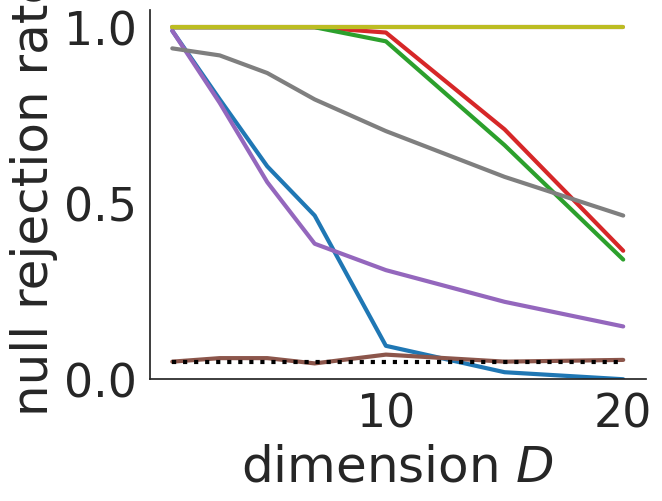
(b) Variance-perturbed Gaussian, 200 repeats

(c) Student-t, 250 repeats

(d) Laplace, 500 repeats

Figure 1: Type I error rate (a) and statistical power (b,c,d) for detecting discrepancies between the unit Gaussian $P$ and the sampling distribution $Q$ (see the main text for details).

We investigate four cases: (a) type I error rate: $Q=\mathcal{N}(0_{d},I_{d})$ (b) statistical power for misspecified variance: $Q=\mathcal{N}(0_{d},\Sigma)$, where $\Sigma_{ij}=0$ for $i\neq j$, $\Sigma_{11}=1.7$ and $\Sigma_{ii}=1$ for $i=2,\ldots,d$, (c) statistical power for misspecified kurtosis: $Q=\mathcal{T}(0,5)$, a standard multivariate student-t distribution with $5$ degrees of freedom, and (d) statistical power for misspecified kurtosis: $q(x)=\prod_{t=1}^{d}\text{Lap}(x_{t}\mid 0,\frac{1}{\sqrt{2}})$, the product of $d$ independent Laplace distributions with variance $1$. Following Huggins and Mackey, (2018), all experiments use $n=1000$ except the multivariate t, which uses $n=2000$.

As seen in Figure 5(a), the type I error rate is generally close to 0.05 even with this finite $n$. Exceptions include RFSD which has decaying type I error rate with increasing $d$, and PSD with $r=4$, which has a slightly over-inflated type I error rate for $d=1$.

As expected, PSD with $r=1$ is incapable of detecting discrepancies with the second (b) or fourth order moments (c,d). Similarly, PSD with $r=2$ and $r=3$ are incapable of detecting discrepancies with the fourth moment (c,d). When the polynomial order is at least as high as the order of the moment in which there are discrepancies, PSD outperforms linear-time methods and is competitive with quadratic-time KSD methods. Specifically, PSD with $r=4$ is the only method to consistently achieve a power of $\approx 1$ in Figures 5(c) and 5(d). In Figure 5(b), PSD with $r=2$ and $r=4$ are the only methods to consistently achieve a power of $1$, while PSD with $r=3$ has a higher statistical power than the competitors at $d=20$.

Next, following Liu et al., (2016) and Jitkrittum et al., (2017), we consider the case where the target $P$ is the non-normalized density of a restricted Boltzmann machine (RBM); the samples $\hat{Q}_{n}$ are obtained from the same RBM perturbed by independent Gaussian noise with variance $\sigma^{2}$. For $\sigma^{2}=0$, $H_{0}:Q=P$ holds, and for $\sigma^{2}>0$ the goal is to detect that the $n=1000$ samples come from the perturbed RBM. Similar to the previous goodness-of-fit test, the null rejection rate for a range of perturbations using 100 repeats is given in Table 1. Notably, PSD with $r=2$ and $r=3$ both outperform linear-time methods and are competitive with quadratic-time methods, showing that PSD is a potentially valuable tool for goodness-of-fit testing in the non-Gaussian setting.

Table 1: Null rejection rates for testing methods at different perturbation levels in the RBM example.

PERTURBATION:	0	0.02	0.04	0.06
RFSD	0.00	0.48	0.93	0.98
FSSD-opt	0.05	0.70	0.96	0.99
IMQ KSD	0.08	0.99	1.00	1.00
Gauss KSD	0.08	0.95	1.00	1.00
PSD r1	0.08	0.51	0.96	0.99
PSD r2	0.06	1.00	1.00	1.00
PSD r3	0.09	0.97	1.00	1.00

4.2 Measure of Sample Quality

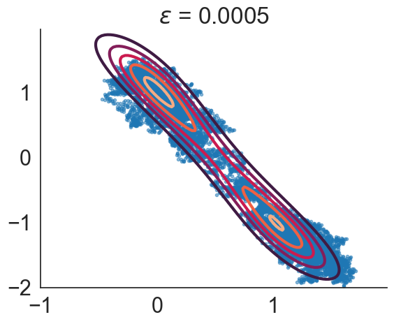
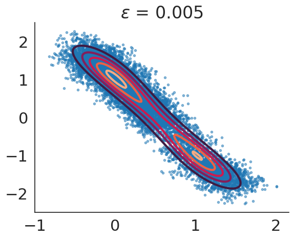
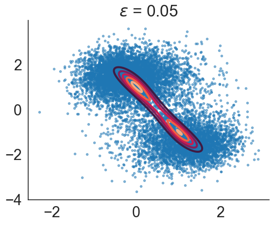
Figure 2: Approximate posterior for mixture example with SGLD for varying step sizes and when sampling from the true posterior using MALA.

Figure 3: Step size selection results for SGLD using various methods.

To demonstrate the advantages of PSD as a measure of discrepancy we follow the stochastic gradient Langevin dynamics (SGLD) hyper-parameter selection setup from Gorham and Mackey, (Section 5.3, 2015). Since no Metropolis-Hastings correction is used, SGLD with constant step size $\epsilon$ is a biased MCMC algorithm that aims to approximate the true posterior. Importantly, the stationary distribution of SGLD deviates more from the target as $\epsilon$ grows, leading to an inflated variance. However, smaller $\epsilon$ decreases the mixing speed of SGLD. Hence, an appropriate choice of $\epsilon$ is critical for accurate posterior estimation.

Similar to the experiments considered in Gorham and Mackey, (2015), Chwialkowski et al., (2016) and Huggins and Mackey, (2018), the target $P$ is the bimodal Gaussian mixture model posterior of Welling and Teh, (2011). We compare the step size selection made by PSD to that of RFSD and IMQ KSD when $n=10000$ samples are obtained using SGLD. Figure 2 shows the performance of SGLD for a variety of step-sizes in comparison with high quality samples obtained using MALA. Figure 3 shows that PSD with $r=2$, $r=3$ and $r=4$ agree with IMQ KSD, selecting $\epsilon=0.005$ which is visually optimal as per Figure 2. Moreover, when utilized as a measure of discrepancy, PSD was around 70 times faster than KSD and around 7 times faster than RFSD.

4.3 Runtime

We now compare the computational cost of computing PSD with that of RFSD and IMQ KSD. Datasets of dimension $d=10$ with the sample size $n$ ranging from $500$ to $10000$ were generated from $P=\mathcal{N}(0_{d},I_{d})$. As seen in Figure 4, even for moderate dataset sizes, the PSD and RFSDs are computed orders of magnitude faster than KSD. While RFSD is faster than PSD with $r=3$ or $r=4$, we have found in Sections 4.1 and 4.2 that PSD can have higher statistical power for detecting discrepancies in moments.

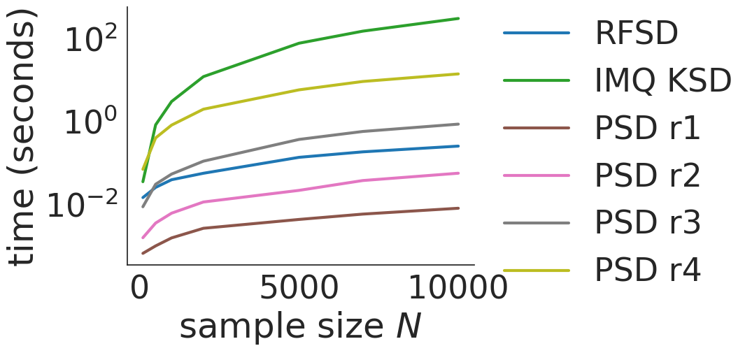
Figure 4: Runtime for various testing methods where $P=\mathcal{N}(0_{d},I_{d})$ with $d=10$.

5 CONCLUSION

Our proposed PSD is a powerful measure of sample quality, particularly for detecting moment convergence. By eliminating the need for extensive calibration, PSD provides a scalable, linear-time solution for goodness-of-fit testing and approximate MCMC tuning. Notably, we have empirically found that the bootstrap PSD test consistently has superior statistical power relative to linear-time competitors, especially in higher dimensions, when the discrepancy can be attributed to one of the first $r$ moments. This makes it a valuable tool for practitioners needing efficient, dependable measures of sample quality, especially in the context of complex Bayesian inference applications. For practitioners using PSD for biased MCMC samplers like SG-MCMC, we recommend using PSD with $r=2$.

We show in Appendix C that in the case of Gaussian $P$ (in the Bernstein-von Mises limit), one can apply any invertible linear transform to the parameters and the method will still detect discrepancies between the original $Q$ and $P$ in the first $r$ moments. We suggest applying whitening or simply standardisation when the variances differ substantially across dimensions. Future work could also consider using alternative norms, for example by maximising subject to the constraint that $\|\beta\|_{1}\leq 1$ or $\|\beta^{\top}W\beta\|_{2}\leq 1$, the latter of which could be used to weight different monomials and therefore different moments.

A further extension could be the use of PSD as a tool to determine in which moments discrepancies between $Q$ and $P$ are occurring. In particular, we could examine $\tau$ and its distribution under $H_{0}$ to obtain an ordering of which monomial terms are contributing the most to the discrepancy.

Acknowledgements

Narayan Srinivasan is supported by the Australian Government through a research training program (RTP) stipend. LFS is supported by a Discovery Early Career Researcher Award from the Australian Research Council (DE240101190). CD is supported by a Future Fellowship from the Australian Research Council (FT210100260). LFS would like to thank Christopher Nemeth and Rista Botha for helpful discussions. Computing resources and services used in this work were provided by the High Performance Computing and Research Support Group, Queensland University of Technology, Brisbane, Australia.

Appendix A Proof of Proposition 1

Proof.

Using the multi-index notation $x^{\alpha}=\prod_{i=1}^{d}x[i]^{\alpha_{i}}$, we have $\mathcal{G}=\text{span}\{x^{\alpha}:\alpha\in\mathbb{N}_{0}^{d},\sum_{i=1}^{d}\alpha_{i}\leq r\}$ for PSD with polynomial order $r$ and

PSD $$=\sqrt{\sum_{\alpha\in\mathbb{N}_{0}^{d}:\sum_{i=1}^{d}\alpha_{i}\leq r}\mathbb{E}_{Q}[\mathcal{A}x^{\alpha}]^{2}}.$$

Thus, $\text{PSD}=0$ if and only if $\mathbb{E}_{Q}[\mathcal{A}x^{\alpha}]=0$ for all $\alpha\in\mathbb{N}_{0}^{d}:\sum_{i=1}^{d}\alpha_{i}\leq r$. We will now proceed by proving that $\mathbb{E}_{Q}[\mathcal{A}x^{\alpha}]=0$ for all $\alpha\in\mathbb{N}_{0}^{d}:\sum_{i=1}^{d}\alpha_{i}\leq r$ (i.e. $\text{PSD}=0$) if and only if the moments of $P$ and $Q$ match up to order $r$.

The condition that $\mathbb{E}_{Q}[\mathcal{A}x^{\alpha}]=0$ for all $\alpha\in\mathbb{N}_{0}^{d}:\sum_{i=1}^{d}\alpha_{i}\leq r$ can be written as a system of ${{d+r}\choose{d}}-1$ linear equations. For each $\alpha$, we wish to understand the conditions under which

$$\mathbb{E}_{Q}[\mathcal{A}x^{\alpha}] =\mathbb{E}_{Q}[\Delta x^{\alpha}+\nabla\log p(x)\cdot\nabla x^{\alpha}]$$

$$=\mathbb{E}_{Q}[\Delta x^{\alpha}+(-\Sigma^{-1}(x-\mu))\cdot\nabla x^{\alpha}]$$

$$=\mathbb{E}_{Q}[\Delta x^{\alpha}]-\mathbb{E}_{Q}[\Sigma^{-1}x\cdot\nabla x^{\alpha}]+\mathbb{E}_{Q}[\Sigma^{-1}\mu\cdot\nabla x^{\alpha}]$$ (12)

$$=0.$$

This uses the property that $P$ is a Gaussian distribution as per the Bernstein-von Mises limit, so $\nabla\log p(x)=-\Sigma^{-1}(x-\mu)$.

Since $P$ decays faster than polynomially in the tails, we can also use the property that $\mathbb{E}_{P}[\mathcal{A}x^{\alpha}]=0$. This leads to a system of ${{d+k}\choose{d}}-1$ linear equations, where for each $\alpha$

$$\mathbb{E}_{P}[\mathcal{A}x^{\alpha}] =\mathbb{E}_{P}[\Delta x^{\alpha}+\nabla x^{\alpha}\cdot(-\Sigma^{-1}(x-\mu))]$$

$$=\mathbb{E}_{P}[\Delta x^{\alpha}]-\mathbb{E}_{P}[\nabla x^{\alpha}\cdot\Sigma^{-1}x]+\mathbb{E}_{P}[\nabla x^{\alpha}\cdot\mu]$$ (13)

$$=0.$$

Subtracting (A) from (A),

$$\mathbb{E}_{Q-P}[\Delta x^{\alpha}]-\mathbb{E}_{Q-P}[\nabla x^{\alpha}\cdot\Sigma^{-1}x]+\mathbb{E}_{Q-P}[\nabla x^{\alpha}\cdot\mu] =0,$$ (14)

where $\mathbb{E}_{Q-P}[f(x)]$ is used as a shorthand for $\mathbb{E}_{Q}[f(x)]-\mathbb{E}_{P}[f(x)]$. Equation (14) combines the condition that $\mathbb{E}_{Q}[\mathcal{A}x^{\alpha}]=0$ with the property that $\mathbb{E}_{P}[\mathcal{A}x^{\alpha}]=0$ into a single system of equations. Our task is to prove that this system of equations holds if and only if the moments of $P$ and $Q$ match up to order $r$. We will do so using proof by induction on the polynomial order $r$.

A.1 Base case ($r=1$)

For $r=1$, $x^{\alpha}$ simplifies to $x_{i}$ for $i\in\{1,\ldots,d\}$. It is simpler in this case to work directly with (A) than to work with (14). For each $i\in\{1,\ldots,d\}$, we have

$$\mathbb{E}_{Q}[\mathcal{A}x_{i}] =0$$

$$\mathbb{E}_{Q}[\Delta x_{i}]-\mathbb{E}_{Q}[\Sigma^{-1}x\cdot\nabla x_{i}]+\mathbb{E}_{Q}[\Sigma^{-1}\mu\cdot\nabla x_{i}] =0$$

$$-\mathbb{E}_{Q}[\Sigma_{i\cdot}^{-1}x]+\mathbb{E}_{Q}[\Sigma_{i\cdot}^{-1}\mu] =0$$

$$\mathbb{E}_{Q}[\Sigma_{i\cdot}^{-1}x] =\Sigma_{i\cdot}^{-1}\mu,$$

where $\Sigma_{i\cdot}^{-1}$ denotes the $i$th row of $\Sigma^{-1}$. Vectorising the above system of equations we have

$$\Sigma^{-1}\mathbb{E}_{Q}[x] =\Sigma^{-1}\mu$$

$$\mathbb{E}_{Q}[x] =\mu.$$

This proves that PSD with $r=1$ is zero if and only if the first order moments (means) of $P$ and $Q$ match.

A.2 Base case ($r=2$)

For $r=2$, $x^{\alpha}$ simplifies to $x_{i}x_{j}$ for $i,j\in\{1,\ldots,d\}$. Following (14), for each $i,j$ we have

$$\mathbb{E}_{Q-P}[\Delta x_{i}x_{j}]-\mathbb{E}_{Q-P}[\Sigma^{-1}x\cdot\nabla x_{i}x_{j}]+\mathbb{E}_{Q-P}[\Sigma^{-1}\mu\cdot\nabla x_{i}x_{j}] =0.$$

The first term is $\mathbb{E}_{Q-P}[\Delta x_{i}x_{j}]=0$ because $\Delta x_{i}x_{j}=2\mathbb{I}_{i=j}$ does not depend on $x$ so the expectations under $P$ and $Q$ match. Similarly, the final term $\mathbb{E}_{Q-P}[\mu\cdot\nabla x_{i}x_{j}]$ disappears because first-order moments match. Thus

$$\mathbb{E}_{Q-P}[\Sigma^{-1}x\cdot\nabla x_{i}x_{j}] =0$$

$$\mathbb{E}_{Q-P}[\Sigma_{i\cdot}^{-1}xx_{j}]+\mathbb{E}_{Q-P}[\Sigma_{j\cdot}^{-1}xx_{i}] =0$$

$$\left(\Sigma^{-1}\mathbb{E}_{Q-P}[xx^{\top}]\right)_{ij}+\left(\Sigma^{-1}\mathbb{E}_{Q-P}[xx^{\top}]\right)_{ji} =0$$

$$\left(\Sigma^{-1}\mathbb{E}_{Q-P}[xx^{\top}]\right)_{ij}+\left(\mathbb{E}_{Q-P}[xx^{\top}]\Sigma^{-1}\right)_{ij} =0$$

$$\left(\Sigma^{-1}A\right)_{ij}+\left(A\Sigma^{-1}\right)_{ij} =0,$$ (15)

where $A=\mathbb{E}_{Q-P}[xx^{\top}]$. Note that $xx^{\top}$ gives all possible second order moments so if $A=0$ then all second order moments match. We need to show that $A=0$ is the only possible solution to this equation.

Let $\Sigma^{-1}=QDQ^{\top}$, where $D$ is the diagonal matrix of eigenvalues with $D_{kk}=\lambda_{k}$ for $k\in\{1,\ldots,d\}$. This is an eigen-decomposition so $Q$ and $Q^{\top}$ are orthogonal ($Q^{\top}=Q^{-1}$). Now, (A.2) holds for all $i,j$ so the vectorised system of linear equations is

$$\Sigma^{-1}A+A\Sigma^{-1} =0$$

$$QDQ^{\top}A+AQDQ^{\top} =0$$

$$DQ^{\top}AQ+Q^{\top}AQD =0$$

$$D\beta+\beta D =0,$$

where $\beta=Q^{\top}AQ$. The third line comes from multiplying by $Q^{\top}$ on the left-hand side and $Q$ on the right-hand side. Consider now the $ij$th element:

$$(D\beta)_{ij}+(\beta D)_{ij} =0$$

$$(\lambda_{i}+\lambda_{j})\beta_{ij} =0.$$

We know that $\lambda_{k}>0$ for all $k\in\{1,\ldots,d\}$ because $\Sigma^{-1}$ is symmetric positive definite, so it must be that $\beta=0$ and therefore $A=0$ is the only solution.

This proves that PSD with $r=2$ if and only if the moments of $P$ and $Q$ match up to order two, i.e. the means and (co)variances match.

A.3 Inductive Step

Suppose that the moments up to and including order $r-1$ match. Noting that $\mathbb{E}_{Q-P}[\Delta x^{\alpha}]$ is of order $r-2$ and $\mathbb{E}_{Q-P}[\nabla x^{\alpha}\cdot\mu]$ is of order $r-1$ and using (14), we have

$$\mathbb{E}_{Q-P}[\nabla x^{\alpha}\cdot\Sigma^{-1}x] =0.$$ (16)

We must show this signifies that the moments of order $r$ must also match.

For a general $r$th order monomial, $x^{\alpha}$ can alternatively be written as $\prod_{m=1}^{r}x_{i_{m}}$ for $i_{m}\in\{1,\ldots,d\}$. Therefore we have

$$\mathbb{E}_{Q-P}[\Sigma^{-1}x\cdot\nabla\prod_{m=1}^{r}x_{i_{m}}]=\sum_{n=1}^{r}\mathbb{E}_{Q-P}[\Sigma_{i_{n}\cdot}^{-1}x\prod_{m=1,m\neq n}^{r}x_{i_{m}}]=0.$$

This can be written in matrix form for all possible multi-indices of order $r$ using Kronecker products:

$$0 =\mathbb{E}_{Q-P}[\overbrace{\Sigma^{-1}x\otimes x^{\top}\otimes x^{\top}\otimes\cdots\otimes x^{\top}}^{r\text{ terms}}]+\mathbb{E}_{Q-P}[x\otimes(x^{\top}\Sigma^{-1})\otimes x^{\top}\otimes\cdots\otimes x^{\top}]+$$

$$\phantom{=+}\mathbb{E}_{Q-P}[x\otimes x^{\top}\otimes(x^{\top}\Sigma^{-1})\otimes\ldots\otimes x^{\top}]+\cdots+\mathbb{E}_{Q-P}[x\otimes x^{\top}\otimes x^{\top}\otimes\ldots\otimes(x^{\top}\Sigma^{-1})].$$

Writing $A=\mathbb{E}_{Q-P}[\overbrace{x\otimes x^{\top}\otimes\cdots\otimes x^{\top}}^{r\text{ terms}}]\in\mathbb{R}^{d\times d^{r-1}}$ and using $(A\otimes B)(C\otimes D)=AB\otimes CD$ provided that one can form the products $AB$ and $CD$, this becomes

$$\Sigma^{-1}A+A(\overbrace{\Sigma^{-1}\otimes I\otimes\cdots\otimes I}^{r-1\text{ terms}})+A(I\otimes\Sigma^{-1}\otimes\cdots\otimes I)+\cdots+A(I\otimes I\otimes\cdots\otimes\Sigma^{-1}) =0.$$

Once again using $\Sigma^{-1}=QDQ^{\top}$, we have

$$QDQ^{\top}A+A(QDQ^{\top}\otimes I\otimes\cdots\otimes I)+A(I\otimes QDQ^{\top}\otimes\cdots\otimes I)+\cdots+A(I\otimes I\otimes\cdots\otimes QDQ^{\top}) =0.$$

Multiplying by $Q^{\top}$ on the left and $(\overbrace{Q\otimes Q\otimes\cdots\otimes Q}^{r-1\text{ terms}})$ on the right

$$0 =DQ^{\top}A(Q\otimes Q\cdots\otimes Q)+Q^{\top}A(QDQ^{\top}\otimes I\otimes\cdots\otimes I)(Q\otimes Q\cdots\otimes Q)$$

$$\phantom{=}+Q^{\top}A(I\otimes QDQ^{\top}\otimes\cdots\otimes I)(Q\otimes Q\cdots\otimes Q)+\cdots+Q^{\top}A(I\otimes I\otimes\cdots\otimes QDQ^{\top})(Q\otimes Q\cdots\otimes Q)$$

$$0 =DQ^{\top}A(Q\otimes Q\cdots\otimes Q)+Q^{\top}A(QD\otimes Q\otimes\cdots\otimes Q)$$

$$\phantom{=}+Q^{\top}A(Q\otimes QD\otimes\cdots\otimes Q)+\cdots+Q^{\top}A(Q\otimes Q\otimes\cdots\otimes QD)$$

$$0 =DQ^{\top}A(Q\otimes Q\cdots\otimes Q)+Q^{\top}A(Q\otimes Q\cdots\otimes Q)(D\otimes I\otimes\cdots\otimes I)$$

$$\phantom{=}+Q^{\top}A(Q\otimes Q\cdots\otimes Q)(I\otimes D\otimes\cdots\otimes I)+\cdots+Q^{\top}A(Q\otimes Q\cdots\otimes Q)(I\otimes I\otimes\cdots\otimes D)$$

$$0 =D\beta+\beta(D\otimes I\otimes\cdots\otimes I)+\beta(I\otimes D\otimes\cdots\otimes I)+\cdots+\beta(I\otimes I\otimes\cdots\otimes D),$$

where $\beta=Q^{\top}A(Q\otimes Q\otimes\cdots\otimes Q)$. Now consider the $ij$th entries in these equations, where $i\in\{1,\ldots,d\}$ and $j\in\{1,\ldots,d^{r-1}\}$. The Kronecker product of diagonal matrices is diagonal, so the terms $(D\otimes I\otimes\cdots\otimes I)$, $(I\otimes D\otimes\cdots\otimes I)$ up to $(I\otimes I\otimes\cdots\otimes D)$ all consist of diagonal matrices with elements of $\lambda$ on the diagonal. The explicit value of $\lambda$ for any given $i$ and $j$ is not important, so for now consider indices $z_{s}\in\{1,\ldots,d\}$ for $s=1,\ldots,r$ which may not be unique. Then we have

$$(\lambda_{z_{1}}+\lambda_{z_{2}}+\cdots\lambda_{z_{k}})\beta_{ij} =0.$$

Since all $\lambda>0$ by positive-definiteness of $\Sigma^{-1}$, we have that $\beta_{ij}=0$ for all $i$ and $j$ and therefore

$$\beta =0$$

$$Q^{\top}A(Q\otimes Q\otimes\cdots\otimes Q) =0$$

$$A =0,$$

where the third line comes from multiplying by $Q$ on the left and $(Q^{\top}\otimes Q^{\top}\otimes\cdots\otimes Q^{\top})$ on the right. We have now shown that $\mathbb{E}_{Q}[\mathcal{A}x^{\alpha}]=0$ for all $\alpha\in\mathbb{N}_{0}^{d}:\sum_{i=1}^{d}\alpha_{i}\leq r$ if and only if the moments of $P$ and $Q$ match up to order $r$. Thus $\text{PSD}=0$ if and only if the moments of $P$ and $Q$ match up to order $r$.

∎

Appendix B Additional Empirical Results

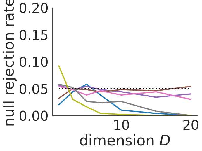
(a) Unit Gaussian (i.e. $Q=P$), 500 repeats

(b) Variance-perturbed Gaussian, 200 repeats

(c) Student-t, 250 repeats

(d) Laplace, 500 repeats

Figure 5: Type I error rate (a) and statistical power (b,c,d) for detecting discrepancies between the unit Gaussian $P$ and the sampling distribution $Q$, using the test based on the asymptotic distribution of the U-statistic.

We reproduce figure 1 in section 4.1 of the main paper by using Corollary 3.0.1 to implement a test based on the asymptotic distribution of the U-statistic, $\widehat{\text{PSD}}^{2}_{u}$. Specifically, we set $P=N(0_{d},I_{d})$ and assess the performance for a variety of $Q$ and $d$ using statistical tests with significance level $\alpha=0.05$. We draw $5000$ samples from the null distribution given in Corollary 3.0.1 using the plugin estimator $\hat{\Sigma}_{q}$. We investigate the four cases described in Section 4 with identical settings as in the main paper.

The results are shown in Figure 5. Primarily, while PSD displays good performance for the variance-perturbed ($r=2$ and $r=4$) and Laplace ($r=4$) experiments, PSD with $r=4$ does not maintain high power in the case of the student-t. Also, we note that the type I error is not well controlled. Further, the asymptotic test can be slower than the bootstrap test due to the computation of the eigenvalues of the covariance matrix (complexity $\mathcal{O}(J^{3})$). This can be improved by considering approximations to the covariance matrix, however this would introduce bias asymptotically.

We recommend the bootstrap procedure for goodness-of-fit testing over the asymptotic test due to its higher statistical power, better control over type I error and lower computational complexity.

Appendix C Using an Invertible Linear Transform

Corollary C.0.1.

Consider PSD applied on the transformed space $y=Wx$, where $W\in\mathbb{R}^{d\times d}$ is an invertible matrix that is independent of $\{x_{i}\}_{i=1}^{N}$. Denote the distribution of $y=Wx$ by $\tilde{Q}$. Using a change of variables, $\nabla_{y}\log\tilde{p}(y)=W^{-\top}\nabla_{x}\log p(x)$. The new discrepancy,

$$\text{PSD}_{W}=\sqrt{\sum_{\alpha\in\mathbb{N}_{0}^{d}:\sum_{i=1}^{d}\alpha_{i}\leq r}\mathbb{E}_{\tilde{Q}}[\Delta_{y}y^{\alpha}+\nabla_{y}\log\tilde{p}(y)\cdot\nabla_{y}y^{\alpha}]^{2}},$$

is zero if and only if the moments of $P$ and $Q$ match up to order $r$.

Proof.

Under the Bernstein-von-Mises limit (or generally for Gaussian targets), $P=\mathcal{N}(\mu,\Sigma)$ so in the transformed space $\tilde{P}=\mathcal{N}(\tilde{\mu},\tilde{\Sigma})$ where $\tilde{\mu}=W\mu$ and $\tilde{\Sigma}=W\Sigma W^{\top}$.

Next, we will show that $\tilde{\Sigma}$ is symmetric positive definite. Since $\tilde{\Sigma}=W\Sigma W^{\top}=\tilde{\Sigma}^{\top}$, $\tilde{\Sigma}$ is symmetric. Since $\Sigma$ is positive-definite, $z^{\top}\tilde{\Sigma}z=z^{\top}W\Sigma W^{\top}z>0$ only requires that we do not have $W^{\top}z=0$ and therefore by invertibility of $W$, that we do not have $z=0$. Thus, $z^{\top}\tilde{\Sigma}z=z^{\top}W\Sigma W^{\top}z>0$ for all non-zero $z\in\mathbb{R}^{d}$, which by definition means that $\tilde{\Sigma}$ is positive-definite.

The assumptions of Proposition 1 (symmetric, positive-definite covariance) are met for this transformed space so for any $r\in\mathbb{N}$ we have

$$\mathbb{E}_{y\sim\tilde{Q}}[\overbrace{y\otimes y^{\top}\otimes\cdots\otimes y^{\top}}^{(r\text{ terms})}] =\mathbb{E}_{y\sim\tilde{P}}[\overbrace{y\otimes y^{\top}\otimes\cdots\otimes y^{\top}}^{(r\text{ terms})}]$$

$$\mathbb{E}_{x\sim Q}[Wx\otimes(Wx)^{\top}\otimes\cdots\otimes(Wx)^{\top}] =\mathbb{E}_{x\sim P}[Wx\otimes(Wx)^{\top}\otimes\cdots\otimes(Wx)^{\top}]$$

$$W\mathbb{E}_{x\sim Q}[x\otimes x^{\top}\otimes\cdots\otimes x^{\top}](W^{\top}\otimes\cdots\otimes W^{\top}) =W\mathbb{E}_{x\sim P}[x\otimes x^{\top}\otimes\cdots\otimes x^{\top}](W^{\top}\otimes\cdots\otimes W^{\top})$$

$$\mathbb{E}_{x\sim Q}[x\otimes x^{\top}\otimes\cdots\otimes x^{\top}] =\mathbb{E}_{x\sim P}[x\otimes x^{\top}\otimes\cdots\otimes x^{\top}].$$

Therefore we have that PSD applied to the transformed $y=Wx$ is equal to zero if and only if the moments of $P$ and $Q$ match up to order $r$.

∎

References

- Anastasiou et al., (2023) Anastasiou, A., Barp, A., Briol, F.-X., Ebner, B., Gaunt, R. E., Ghaderinezhad, F., Gorham, J., Gretton, A., Ley, C., Liu, Q., Mackey, L., Oates, C. J., Reinert, G., and Swan, Y. (2023). Stein’s method meets computational statistics: A review of some recent developments. Statistical Science, 38(1):120 – 139.
- Arcones and Gine, (1992) Arcones, M. A. and Gine, E. (1992). On the Bootstrap of U and V Statistics. The Annals of Statistics, 20(2):655–674.
- Assaraf and Caffarel, (1999) Assaraf, R. and Caffarel, M. (1999). Zero-variance principle for Monte Carlo algorithms. Physical Review Letters, 83(23):4682–4685.
- Barbour, (1990) Barbour, A. D. (1990). Stein’s method for diffusion approximations. Probability theory and related fields, 84(3):297–322.
- Berlinet and Thomas-Agnan, (2004) Berlinet, A. and Thomas-Agnan, C. (2004). Reproducing Kernel Hilbert Spaces in Probability and Statistics. Springer US, Boston, MA.
- Bhattacharya et al., (2024) Bhattacharya, A., Linero, A., and Oates, C. J. (2024). Grand challenges in bayesian computation.
- Chwialkowski et al., (2016) Chwialkowski, K., Strathmann, H., and Gretton, A. (2016). A kernel test of goodness of fit. In Balcan, M. F. and Weinberger, K. Q., editors, Proceedings of The 33rd International Conference on Machine Learning, volume 48 of Proceedings of Machine Learning Research, pages 2606–2615, New York, New York, USA. PMLR.
- Chwialkowski et al., (2015) Chwialkowski, K. P., Ramdas, A., Sejdinovic, D., and Gretton, A. (2015). Fast two-sample testing with analytic representations of probability measures. In Cortes, C., Lawrence, N., Lee, D., Sugiyama, M., and Garnett, R., editors, Advances in Neural Information Processing Systems, volume 28. Curran Associates, Inc.
- Gorham and Mackey, (2015) Gorham, J. and Mackey, L. (2015). Measuring sample quality with Stein’s method. In Cortes, C., Lawrence, N., Lee, D., Sugiyama, M., and Garnett, R., editors, Advances in Neural Information Processing Systems, volume 28. Curran Associates, Inc.
- Gorham and Mackey, (2017) Gorham, J. and Mackey, L. (2017). Measuring sample quality with kernels. In Precup, D. and Teh, Y. W., editors, Proceedings of the 34th International Conference on Machine Learning, volume 70 of Proceedings of Machine Learning Research, pages 1292–1301. PMLR.
- Huggins, (2018) Huggins, J. (2018). rfsd package. https://bitbucket.org/jhhuggins/random-feature-stein-discrepancies/src/master/.
- Huggins and Mackey, (2018) Huggins, J. and Mackey, L. (2018). Random feature Stein discrepancies. In Bengio, S., Wallach, H., Larochelle, H., Grauman, K., Cesa-Bianchi, N., and Garnett, R., editors, Advances in Neural Information Processing Systems, volume 31. Curran Associates, Inc.
- Hušková and Janssen, (1993) Hušková, M. and Janssen, P. (1993). Consistency of the generalized bootstrap for degenerate u-statistics. The Annals of Statistics, 21(4):1811–1823.
- Jitkrittum, (2019) Jitkrittum, W. (2019). kernel-gof package. https://github.com/wittawatj/kernel-gof.
- Jitkrittum et al., (2017) Jitkrittum, W., Xu, W., Szabo, Z., Fukumizu, K., and Gretton, A. (2017). A linear-time kernel goodness-of-fit test. In Guyon, I., Luxburg, U. V., Bengio, S., Wallach, H., Fergus, R., Vishwanathan, S., and Garnett, R., editors, Advances in Neural Information Processing Systems, volume 30. Curran Associates, Inc.
- Kanagawa et al., (2022) Kanagawa, H., Barp, A., Gretton, A., and Mackey, L. (2022). Controlling moments with kernel Stein discrepancies. arXiv preprint arXiv:2211.05408.
- Leucht and Neumann, (2013) Leucht, A. and Neumann, M. (2013). Dependent wild bootstrap for degenerate uu- and vv-statistics. Journal of Multivariate Analysis, 117:257–280.
- Liu et al., (2016) Liu, Q., Lee, J., and Jordan, M. (2016). A kernelized Stein discrepancy for goodness-of-fit tests. In Balcan, M. F. and Weinberger, K. Q., editors, Proceedings of The 33rd International Conference on Machine Learning, volume 48 of Proceedings of Machine Learning Research, pages 276–284, New York, New York, USA. PMLR.
- Mira et al., (2013) Mira, A., Solgi, R., and Imparato, D. (2013). Zero variance Markov chain Monte Carlo for Bayesian estimators. Statistics and Computing, 23(5):653–662.
- Müller, (1997) Müller, A. (1997). Integral probability metrics and their generating classes of functions. Advances in Applied Probability, 29(2):429–443.
- Nemeth and Fearnhead, (2021) Nemeth, C. and Fearnhead, P. (2021). Stochastic gradient Markov chain Monte Carlo. Journal of the American Statistical Association, 116(533):433–450.
- Rahimi and Recht, (2007) Rahimi, A. and Recht, B. (2007). Random features for large-scale kernel machines. In Platt, J., Koller, D., Singer, Y., and Roweis, S., editors, Advances in Neural Information Processing Systems, volume 20. Curran Associates, Inc.
- Roberts and Tweedie, (1996) Roberts, G. O. and Tweedie, R. L. (1996). Exponential convergence of Langevin distributions and their discrete approximations. Bernoulli, 2(4):341–363.
- Serfling, (2009) Serfling, R. J. (2009). Approximation theorems of mathematical statistics. John Wiley & Sons.
- South et al., (2022) South, L. F., Karvonen, T., Nemeth, C., Girolami, M., and Oates, C. J. (2022). Semi-exact control functionals from Sard’s method. Biometrika, 109(2):351–367.
- South et al., (2023) South, L. F., Oates, C. J., Mira, A., and Drovandi, C. (2023). Regularized zero-variance control variates. Bayesian Analysis, 18(3):865 – 888.
- Stein, (1972) Stein, C. (1972). A bound for the error in the normal approximation to the distribution of a sum of dependent random variables. In Proceedings of the Sixth Berkeley Symposium on Mathematical Statistics and Probability, Volume 2: Probability Theory, volume 6.2, pages 583–603. University of California Press.
- Welling and Teh, (2011) Welling, M. and Teh, Y. (2011). Bayesian learning via stochastic gradient langevin dynamics. In Proceedings of the 28th International Conference on Machine Learning, pages 681–688.