Learning Hidden Physics and System Parameters with Deep Operator Networks

Abstract

Big data is transforming scientific progress by enabling the discovery of novel models, enhancing existing frameworks, and facilitating precise uncertainty quantification, while advancements in scientific machine learning complement this by providing powerful tools to solve inverse problems to identify the complex systems where traditional methods falter due to sparse or noisy data. We introduce two innovative neural operator frameworks tailored for discovering hidden physics and identifying unknown system parameters from sparse measurements. The first framework integrates a popular neural operator, DeepONet, and a physics-informed neural network to capture the relationship between sparse data and the underlying physics, enabling the accurate discovery of a family of governing equations. The second framework focuses on system parameter identification, leveraging a DeepONet pre-trained on sparse sensor measurements to initialize a physics-constrained inverse model. Both frameworks excel in handling limited data and preserving physical consistency. Benchmarking on the Burgers’ equation and reaction-diffusion system demonstrates state-of-the-art performance, achieving average $L_{2}$ errors of $\mathcal{O}(10^{-2})$ for hidden physics discovery and absolute errors of $\mathcal{O}(10^{-3})$ for parameter identification. These results underscore the frameworks’ robustness, efficiency, and potential for solving complex scientific problems with minimal observational data.

1 Introduction

Recent advances in machine learning, coupled with innovative data recording and sensor technologies, are revolutionizing our understanding of complex systems across scientific and engineering domains. Traditional approaches often struggle to capture the intricate dynamics of systems in fields like neuroscience, epidemiology, and materials science, where direct measurement or explicit modeling proves challenging. The integration of statistical learning techniques with classical applied mathematics has emerged as a powerful approach to bridging this knowledge gap. Consider, for example, the challenge of understanding fluid dynamics [1] in aerospace engineering or predicting cardiovascular blood flow in medical research [2, 3] or predicting failure in materials [4]. These systems are characterized by nonlinear interactions and multiple interdependent variables that defy simple, first-principles modeling. Machine learning offers a transformative solution, enabling researchers to develop sophisticated mathematical models that directly emerge from empirical data. The landscape of data-driven dynamical systems discovery is rich and multifaceted, encompassing diverse methodological innovations. Researchers have developed approaches such as Equation-free modeling [5], deep learning techniques [6], non-linear regression [7], empirical dynamic modeling [8], automated dynamics inference [9], symbolic regression [10], and Koopman analysis [11] to address the fundamental challenge of modeling complex systems with incomplete knowledge and limited observational data.

A critical frontier in this domain is discovering closed-form mathematical models of real-world systems described by partial differential equations (PDEs) and identifying crucial system parameters from sparse, spatiotemporally scattered data. Traditional approaches have struggled to bridge the gap between theoretical understanding and practical measurement. Several prominent approaches have emerged to address these challenges. Existing methods like Sparse Identification of Non-linear Dynamics [12] (SINDy) and Deep Hidden Physics Models [6] (DHPM) have made significant strides, but they face inherent limitations. SINDy approximates system behavior using sparse linear combinations of predefined candidate terms, but the framework requires prior knowledge of system non-linearities and sensitivity to measurement noise. Deep Hidden Physics Models (DHPM) offers a promising alternative by utilizing two deep neural networks. One network captures the system state, while another approximates the unknown physics of the model. The DHPM framework demonstrates remarkable stability, leveraging automatic differentiation techniques to compute gradient terms, thus effectively bypassing the numerical differentiation challenges inherent in traditional approaches. Deep Hidden Physics Models (DHPM) offer improved stability through dual neural networks - one capturing system state, another approximating unknown physics - but cannot identify unknown system parameters from labeled datasets.

Physics-Informed Neural Networks (PINNs) [13, 14, 15] marked a breakthrough in parameter estimation by introducing innovative functional approximation techniques. These methods simultaneously minimize both the residual loss from governing PDEs and the data loss from sparse sensor recordings, demonstrating success across diverse applications - from estimating hemodynamic parameters in cardiovascular systems [16] to reconstructing elasticity fields in heterogeneous materials [4], as well as inferring flow parameters in fluid mechanics [17, 18]. However, a fundamental limitation persists: existing methods typically require re-training and re-evaluation for each system parameter variation, limiting their generalizability and computational efficiency.

This persistent challenge motivates the need for more robust and adaptable modeling techniques. Motivated by these challenges, this study introduces two complementary frameworks:

1. The Deep Hidden Physics Operator (DHPO) network - a generalized operator identified from minimal labeled datasets spanning various system conditions. This framework uniquely integrates DHPM [6] with neural operators [19], specifically deep operator networks, to model system dynamics with partially known physics.

2. A physics-informed operator-learning framework that identifies system parameters for sparse sensor recordings across PDE families, requiring no additional labeled dataset and operating in a semi-supervised approach.

Both these frameworks build upon recent advances in neural operators [20] designed to learn the mappings between infinite dimensional functional spaces, thus facilitating generalization abilities. There are numerous neural operators, which can be categorized into meta-architectures, such as deep operator networks (DeepONet) [19], and operators based on integral transforms, including the Fourier neural operator (FNO) [21], wavelet neural operator (WNO) [22], graph kernel network (GKN) [23], convolutional neural operator [24], and Laplace neural operator (LNO) [25], basis-to-basis framework [26], and the resolution-independent neural operator [27] among others. Among the various neural operators developed, in this work, we consider the DeepONet for its architectural flexibility. Its architecture, inspired by the universal approximation theorem for operators [28], consists of a branch network that encodes varying input functions and a trunk network that encodes spatio-temporal coordinates. Since its first appearance, vanilla DeepONet architecture has been employed to tackle challenging problems involving complex high-dimensional dynamical systems [29, 30, 31, 32]. In addition, extensions of DeepONet have been recently proposed in the context of integration of multiple-input continuous operators [33, 34], hybrid transferable numerical solvers [35, 36], transfer learning [37], physics-informed (PI) learning to satisfy the underlying PDE [38, 20, 39], and multi-task learning framework [40]. Recent advancements have significantly improved its capabilities, including efficient training strategies [41], Seperable PI-DeepONet’s efficient PDE solving [39], RI-DeepONet for resolution-independent training [27], Geom-DeepONet’s 3D geometry prediction [42], and L-DeepONet’s for learning operators in latent space mapping [43]. These developments have enhanced computational efficiency and predictive accuracy across diverse scientific domains. In this study, we employ the vanilla DeepONet as our foundational framework.

These advancements represent a significant step toward robust and efficient modeling of complex dynamical systems with limited observational data. By pushing the boundaries of data-driven scientific modeling, the proposed frameworks offer new opportunities for understanding and predicting intricate system behaviors across various scientific and engineering domains. The remainder of the paper is organized as follows. Section 2 outlines the framework for building surrogates for hidden physics discovery and parameter identification. Section 3 demonstrates the applicability of the proposed framework using benchmark examples. Section 4 summarizes our study and highlights potential future research directions.

2 Physics Discovery and Parameter Identification using Neural Operators

The successful application of deep learning in physical sciences hinges on two critical capabilities: discovering underlying physics from data and identifying system parameters that govern physical processes. Traditional approaches often struggle with generalization across different physical scenarios and require extensive data collection. In this section, we present two frameworks that address these challenges by leveraging DeepONet: first, an innovative approach for discovering physical laws that can generalize across multiple PDE systems, and second, an operator framework for system parameter identification that efficiently handles inverse problems in physical systems.

2.1 Deep Hidden Physics Operator (DHPO) - Discovering physics using DeepONet

Building upon the concept of deep hidden physics models (DHPM) introduced by Raissi et al. [6], we introduce deep hidden physics operator (DHPO) - a framework that leverages the power of operator learning to discover underlying physical laws. While DHPM has proven effective in learning physics from data corresponding to a single PDE system under varying boundaries or initial conditions, our approach extends this capability to learn from multiple PDE systems simultaneously.

Consider a general nonlinear PDE of the form:

$$\frac{\partial{u}}{\partial{t}}=\mathcal{N}(t,x,u,u_{x},u_{xx},..)+f(x),$$ (1)

for $x\in\Omega,t\in[0,T],u:\Omega\times t\rightarrow\mathbb{R}$. Here, $\mathcal{N}$ represents the unknown physics operator we aim to discover, and $f(x)$ is a variable source term. Our framework, DHPO, employs a DeepONet architecture consisting of two primary components: a branch network that processes the input function $f(x)$ at fixed sensor locations, and a trunk network that handles the spatio-temporal coordinates $(x,t)$. The solution field $u(x)$ is approximated through the interaction of these networks via a dot product operation. The gradient, $u_{t},u_{x},u_{xx}$, is computed using the automatic differentiation approach. To discover the underlying physics, we introduce a hidden physics neural network that approximates $\mathcal{N}$ by taking the tuple $[u,u_{x},u_{xx}]$ as inputs. This network learns to represent the unknown terms in the PDE while maintaining the interpretability of the discovered physics. The training of this framework is governed by a composite loss function that encompasses:

1. Initial condition constraints:

   $$\mathcal{L}_{ic}=\frac{1}{N_{ic}b}\sum_{i=1}^{b}\sum_{j=1}^{N_{ic}}|u_{d}(x_{j}^{i},0)-u(x_{j}^{i},0)|^{2},$$ (2)

2. Boundary condition constraints:

   $$\mathcal{L}_{bc}=\frac{1}{N_{bc}b}\sum_{i=1}^{b}\sum_{j=1}^{N_{bc}}|u_{d}(0,t_{j}^{i})-u(0,t_{j}^{i})|^{2}+|u_{d}(1,t_{j}^{i})-u(1,t_{j}^{i})|^{2},$$ (3)

3. PDE residual:

   $$\mathcal{L}_{eqn}=\frac{1}{N_{Coll}b}\sum_{i=1}^{b}\sum_{j=1}^{N_{Coll}}|\left(\frac{\partial u}{\partial t}\right)_{(x_{j}^{i},t_{j}^{i})}-\left(\mathcal{N}(u,u_{x},u_{xx})\right)_{(x_{j}^{i},t_{j}^{i})}-f(x_{j}^{i})|^{2},$$ (4)

4. Data fidelity:

   $$\mathcal{L}_{data}=\frac{1}{N_{d}b}\sum_{i=1}^{b}\sum_{j=1}^{N_{d}}|u(x_{j}^{i},t_{j}^{i})-u_{d}(x_{j}^{i},t_{j}^{i})|^{2},$$ (5)

where $u_{d}(x_{j}^{i},t_{j}^{i})$ and $u(x_{j}^{i},t_{j}^{i})$ denote the reference and predicted solutions at the $j^{th}$ point for the $i^{th}$ sample, respectively. The total loss function combines these components and is defined as:

$$\mathcal{L}_{total}=\mathcal{L}_{ic}+\mathcal{L}_{bc}+\mathcal{L}_{eqn}+\mathcal{L}_{data}.$$ (6)

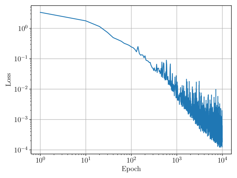
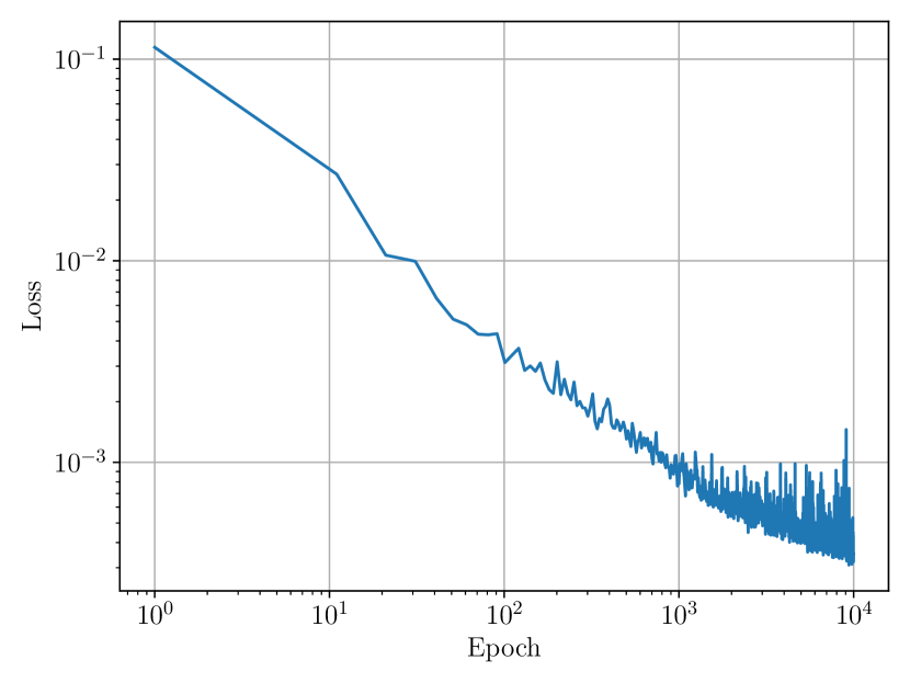
Figure 1: Loss function over the training process of optimal model: (a) Reaction diffusion equation with $N_{train}=500,N_{d}=500.$ (b) Burgers’ equation with $N_{train}=1000,N_{d}=500.$

The parameters of the trunk, branch, and hidden physics networks are optimized simultaneously by minimizing $\mathcal{L}_{total}$. A schematic of the DHPO framework is shown in Figure 1 and the detailed training procedure is presented in Algorithm 1.

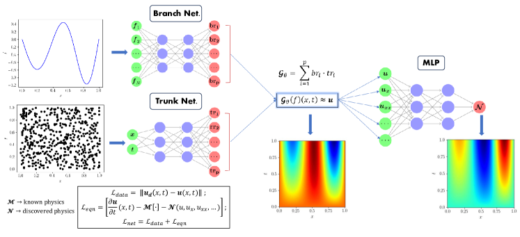
Figure 1: Architecture of the proposed Deep Hidden Physics Operator framework developed to discover the unknown physics leveraging sparsely labeled dataset. The DeepONet learns the solution operator for varying system conditions to predict the desired output. The solution as well as the gradients are considered as inputs to the MLP and it predicts the unknown physics. The entire framework is trained in a single training session with physics loss as defined in Equation 4 and the data loss.

Our framework improves upon traditional DHPM through enhanced generalization that simultaneously handles multiple PDE systems across diverse input functions, boundary conditions, and geometries without retraining. It achieves improved data efficiency by leveraging physics-informed constraints and knowledge transfer, enabling learning from sparse or noisy measurements. The approach maintains increased interpretability, allowing direct extraction of governing equations and insights into physical term importance. Computational advantages emerge from physics-guided optimization, leading to faster convergence, better-conditioned loss landscapes, and reduced computational resources, delivering stable and consistent predictions across varying data scenarios and out-of-distribution conditions.

2.2 System Parameter Identification using DeepONet

Building upon our proposed architecture, we present a modified framework for parameter estimation in governing PDEs through surrogate modeling. While the underlying physics are known in this scenario, our objective is to determine the system parameters that govern the process (i.e., solving the parameter estimation inverse problem). Figure 2 illustrates the schematic of this modified architecture. For this framework, we have considered cases with just sensor recordings and no additional labeled datasets.

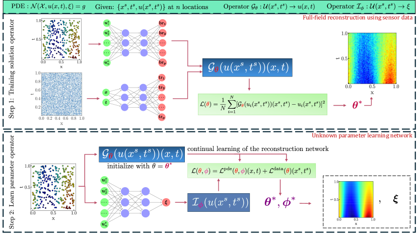
Figure 2: Schematic representation of the proposed architecture for unknown system parameters identification, $\nu$ for the Burger’s equation. In the schematic, $u^{s}$ denotes the known velocity field at fixed sensor locations. In step 1, a data-driven DeepONet is trained with loss defined at just the sensor locations to reconstruct the field based on sparse measurements. In the second step, the trained DeepONet is given a warm start, and the learning of the solution is improved in conjunction with an MLP which predicts the unknown $\nu$ employing a physics loss. $\bm{\theta}^{*},\bm{\phi}^{*}$ are the optimized parameters of the networks.

The framework consists of two key components. First, a DeepONet is pre-trained to learn the forward mapping from sparse input data to the complete solution field. Second, we introduce an additional MLP designed to learn the inverse mapping from the solution space to the parameter space. These two networks – the DeepONet and MLP – are then trained through continual learning, using the PDE residual as the primary loss term. To ensure solution accuracy and physical consistency, we incorporate additional loss terms for known data.

The fundamental advantage of this framework lies in its ability to simultaneously learn both forward and inverse mappings for any given physical system, without any additional labeled data beyond the sensor measurements. This dual-surrogate approach enables efficient parameter estimation while maintaining physical consistency through the embedded governing equations.

1 Inputs: sensor measurements $f(x^{s})$ and $u(x^{s},t^{s})$ at $n$ fixed locations, collocation points $x,t$ , partially known physics $\mathcal{M}$, initial conditions, boundary conditions

2

3Initialize DeepONet $\mathcal{G}_{\bm{\theta}}$ with:

4          Branch network: process sensor inputs $f(x^{s})$

5          Trunk network: process coordinates $(x,t)$

6 Initialize MLP network for physics discovery with $\phi$

7 while not converged do

8       for each batch of sensor data do

9             Forward pass through DeepONet

10             $u_{\text{pred}}$ = $\mathcal{G}_{\bm{\theta}}(f(x^{s})(x,t))$

11             $u_{\text{ic}}$ = $\mathcal{G}_{\bm{\theta}}(f(x^{s})(x,0))$

12             $u_{\text{bc}}$ = $\mathcal{G}_{\bm{\theta}}(f(x^{s})(x_{\text{bc}},t))$

13             Compute gradients

14             $u_{x_{\text{pred}}}=du_{\text{pred}}/dx$

15             $u_{xx_{\text{pred}}}=d^{2}u_{\text{pred}}/dx^{2}$

16             $\cdots$

17             Forward pass through MLP

18             $\mathcal{N}=\text{MLP}(u_{\text{pred}},u_{x_{\text{pred}}},u_{xx_{\text{pred}}},...)$

19            Compute loss

20             $\mathcal{L}^{\text{pde}}=\frac{1}{N}\sum_{i=1}^{N}||\mathcal{N}_{i}+\mathcal{M}_{i}-f(x^{s})_{i}||^{2}$   physics loss

21             $\mathcal{L}^{\text{ic}}=\frac{1}{N}\sum_{i=1}^{N}||u_{\text{ic}_{i}}-u(x,0)||^{2}$   initial condition loss

22             $\mathcal{L}^{\text{bc}}=\frac{1}{N}\sum_{i=1}^{N}||u_{\text{bc}_{i}}-u(x_{\text{bc}},t)||^{2}$   boundary condition loss

23             $\mathcal{L}^{\text{data}}=\frac{1}{N}\sum_{i=1}^{N}||u_{\text{pred}_{i}}-u(x^{s},t^{s})||^{2}$   data loss

24             $\mathcal{L}(\bm{\theta},\phi)=\mathcal{L}^{\text{pde}}(\bm{\theta},\phi)(x,t)+\mathcal{L}^{\text{ic}}(\bm{\theta})(x,0)+\mathcal{L}^{\text{bc}}(\bm{\theta})(x_{\text{bc}},t)+\mathcal{L}^{\text{data}}(\bm{\theta})(x^{s},t^{s})$

25             Backpropagate and update $\bm{\theta}$ and $\phi$ using Adam

26       end for

27      

28 end while

29Final optimized $\theta$, $\phi$

$\theta^{*}$, $\phi^{*}$ = argmin $\mathcal{L}(\theta,\phi)$

Algorithm 1 Training Scheme for the deep Hidden Physics Operator (DHPO).

1 Inputs: sensor measurements $u(x^{s},t^{s})$ at $n$ fixed locations, collocation points $x,t$ , PDE $\mathcal{N}(\mathcal{X},u(x,t),\xi)$

2 Step 1: Training solution operator $\mathcal{G}_{\bm{\theta}}$

3 Initialize DeepONet $\mathcal{G}_{\bm{\theta}}$ with:

4          Branch network: process sensor inputs $u(x^{s},t^{s})$

5          Trunk network: process coordnates $(x,t)$

6 while not converged do

7       for each batch of sensor data do

8             Forward pass through DeepONet at sensor locations

9             prediction = $\mathcal{G}_{\bm{\theta}}(u(x^{s},t^{s})(x^{s},t^{s}))$

10             Compute loss

11             $\mathcal{L}(\theta)=\frac{1}{N}\sum_{i=1}^{N}||\text{prediction}_{i}-u_{i}(x^{s},t^{s})||^{2}$

12            

13            Backpropagate and update $\theta$ using Adam

14       end for

15      

16 end while

17Store optimised $\bm{\theta}$

18       $\bm{\theta}^{*}=\text{ argmin}\mathcal{L}(\bm{\theta})$

19 Step 2: Learn parameter operator $\mathcal{I}_{\bm{\phi}}$

20 Initialize DeepONet $\mathcal{G}_{\bm{\theta}}$ with $\bm{\theta}=\bm{\theta}^{*}$ from step 1.

21 Initialize Parameter network $\mathcal{I}_{\phi}$: maps sensor data $\{u(x^{s},t^{s})\}$ to unknown parameter $\xi$

22 while not converged do

23       for each batch of data do

24             Forward pass through both networks

25             $u_{\text{pred}}$ = $\mathcal{G}_{\bm{\theta}}(u(x^{s},t^{s})(x,t))$

26             $\xi_{\text{pred}}=\mathcal{I}_{\bm{\phi}}(u(x^{s},t^{s}))$

27             Compute combine loss

28             $\mathcal{L}^{\text{pde}}=\frac{1}{N}\sum_{i=1}^{N}||\mathcal{N}(\mathcal{X},u_{\text{pred}_{i}},\xi_{\text{pred}_{i}})-g_{i}||^{2}$   physics loss

29             $\mathcal{L}^{\text{data}}=\frac{1}{N}\sum_{i=1}^{N}||u_{\text{pred}_{i}}-u(x^{s},t^{s})||^{2}$   data loss

30             $\mathcal{L}(\bm{\theta},\bm{\phi})=\mathcal{L}^{\text{pde}}(\bm{\theta},\bm{\phi})(x,t)+\mathcal{L}^{\text{data}}(\bm{\theta})(x^{s},t^{s})$

31             Back-propagate and update $\bm{\theta}$ and $\bm{\phi}$ using Adam

32       end for

33      

34 end while

35

36Final optimized $\bm{\theta}$, $\bm{\phi}$

$\bm{\theta}^{*}$, $\bm{\phi}^{*}$ = argmin $\mathcal{L}(\bm{\theta},\bm{\phi})$

Algorithm 2 Training Scheme to obtain an operator framework for system parameter identification.

We have consider the Loss tolerance $\epsilon$ of $\mathcal{O}(10^{-3})$. To measure the deviation of the predicted solution from reference we use a metric known as relative $L_{2}$ Error which is defined as,

$$\text{relative}\ L_{2}\ \text{Error}=\frac{\sqrt{\sum_{i=1}^{N}|u_{i}-u_{i}^{*}|^{2}}}{\sqrt{\sum_{i=1}^{N}|u_{i}^{*}|^{2}}}$$ (7)

where $u^{*},\;u$ are the reference and the predicted solution respectively. We also define, the error distribution by $\mu\pm\sigma$, where $\mu,\sigma$ are mean and standard deviation of rel. $L_{2}$ errors.

3 Illustrative Problems

To examine our approach, we perform tests on two examples including the Reaction Diffusion equation and Burger’s equation. The input function $f$ acts as the source term for the reaction-diffusion system and initial condition for the burgers’ equation.

3.1 Reaction Diffusion System

We first examine our approaches using a reaction-diffusion equation, which models various physical phenomena in nature such as oscillating chemical concentrations and spatial waves as seen in the Belousov-Zhabotinsky reaction, population dynamics, pattern formation in biological systems and morphology in crystals and alloys [44]. The following equation describes the spatiotemporal evolution of the system and is given by:

$$\begin{split}&\frac{\partial u}{\partial t}(x,t)=D\frac{\partial^{2}u}{\partial x^{2}}(x,t)+Ku^{2}(x,t)+f(x)\text{ on }\ \Omega:(x,t)\in[0,1]^{2},\\ &IC:u(x,0)=0,\\ &BC:u(0,t)=u(1,t)=0,\\ \end{split}$$ (8)

where $D$ and $K$ denote the diffusion and the reaction coefficients, respectively. In Equation 8, IC denotes the initial condition and BC denotes the Dirichlet boundary condition. Going forward, we will first present the results of discovering the unknown physics using DeepONet, followed by presenting the results of employing DeepONet to characterize the diffusion coefficient of the system using sparse measurements.

Discovering physics using DeepONet We re-write Equation 8 to denote the known and the unknown part of the PDE, as

$$\frac{\partial u}{\partial t}=\mathcal{N}(u,u_{x},u_{xx})+f(x),$$ (9)

we assume that we know the time derivative of the problem and the remaining part of the governing equation shown in Equation 8 is unknown as well as approximated by $\mathcal{N}$, employing the proposed deep hidden physics framework within DeepONet. Our objective is to learn a solution operator $\mathcal{G}_{\bm{\theta}}$ that maps the source term $f(x)$ to the solution field $u(x,t)$ using partially known physics and sparse labeled data. For this setup, we have used $D=0.01$ $K=0.01$. To generate the training and testing data, the system in Equation 8 was solved using the finite difference method, with a spatial resolution of $\delta x=0.01$ units and a time step of $\delta t=0.001$ units. The final solution was evaluated on a $101\times 101$ grid in the space-time domain. We investigate three different input function spaces for source term $f(x)$. We train the model only using sine basis functions and test for all three function spaces.

• Sine Basis Functions:

  $$f(x)=\sum_{k=1}^{N_{f}}A_{k}sin(\pi kx),$$ (10)

  where $A_{k}$ are coefficients from a Gaussian normal distribution with mean 0 and variance 1 and the number of frequencies $N_{f}=5$.

• Gaussian Random Fields (GRFs):

  $$GRF(x)\sim{\mathcal{G}(0,k_{l}(x_{1},x_{2}))},$$ (11)

  with RBF kernel $k_{l}(x_{1},x_{2})=exp(-||x_{1}-x_{2}||^{2}/(2l^{2}))$ with a length-scale parameter $l>0$. The $l$ determines the oscillatory nature of the sampled function, a lower value of $l$ leads to higher oscillations. We consider GRFs with RBF kernel length-scale of 0.2, unlike sine basis functions GRFs are not zero at boundaries.

• Modified GRFs:

  $$\textnormal{Modified}\ GRF(x)=\alpha(x-x^{2})GRF(x)$$ (12)

  where $\alpha=8.0$ ensures similar scale as sine basis functions.

To train the framework, the collocation points in the differential equation, initial conditions, and boundary conditions are defined as $N_{Coll}$, $N_{ic}$, and $N_{bc}$, respectively. These points are randomly generated for each sample using Latin hypercube sampling [45], creating synthetic domain data that can vary at each gradient descent step. The training process is shown in Algorithm 1. For this problem, we use $N_{Coll}=2000$, $N_{ic}=200$, and $N_{bc}=250$. To determine the optimal amount of known labeled dataset required, we experiment with data point sets $N_{d}=\{200,500\}$ and training sample sets $N_{train}=\{50,100,200,500\}$, with a fixed number of test samples, $N_{test}=1000$.

The branch net takes the source term discretized at 101 spatial sensor locations, while the trunk net takes the spatial and temporal locations while the hidden physics MLP takes the solution $u$ and the corresponding spatial gradients, $u,u_{x},$ and $u_{xx}$ as inputs to output the prediction $\mathcal{N}$ for RHS in Equation 9. The optimal model was found using training size of $N_{train}=500,N_{d}=500$. The loss curve over the training process is shown in Figure 1(a). The mean test relative $L_{2}$ error for each of the cases is presented in Table 1.

Table 1: Reaction Diffusion system: Mean and standard deviation of the test error for all the three different input function spaces for the source term, $f(x)$. The experiments were carried out for five independent runs.

Method	Test Error (Mean $\pm$ Std)
Sine basis	$0.01742\pm 0.007142$
GRF	$0.14039\pm 0.09857$
Modified GRF	$0.04028\pm 0.03121$

Using sine basis functions for the source term yields the highest prediction accuracy among tested methods. Figure 3(a) illustrates the mean test error over various sample sizes and training data points, while Figure 3(b) shows the distribution of test errors for this optimal model. We further evaluate the model’s predictive capability on unseen sine basis source terms as defined in Equation 10. As shown in Figure 5, the model accurately predicts both the solution $u$ and the hidden physics terms $\mathcal{N}$, aligning closely with ground truth values. The inferred hidden physics term is given by

$$\mathcal{N}\approx D\frac{\partial^{2}u}{\partial x^{2}}+Ku^{2}.$$

Unlike the sine basis, Gaussian random fields (GRFs) do not approach zero at the boundaries, leading to higher deviations in the predicted solution and physics terms, particularly at the boundaries (see Figure 6). Figure 4(a) illustrates the test error distribution for GRFs evaluated with the model trained with sine basis. In contrast, modified GRFs, which are zero at the boundaries similar to sine basis functions, achieve comparable prediction accuracy. Figure 7 shows that, with modified GRFs, the model accurately predicts both $u$ and the hidden physics terms, closely matching the ground truth. The test error distribution for modified GRFs is provided in Figure 4(b).

Additionally, we assess the model’s performance on GRFs by varying the length-scale parameter $l$ of the RBF kernel with values $l\in\{0.1,0.15,0.20,0.40,0.60\}$. As expected, Table 2 demonstrates that prediction error increases as the length scale decreases. However, for out-of-distribution functions with boundary values approaching zero, the model maintains relatively higher accuracy compared to cases with non-zero boundary conditions.

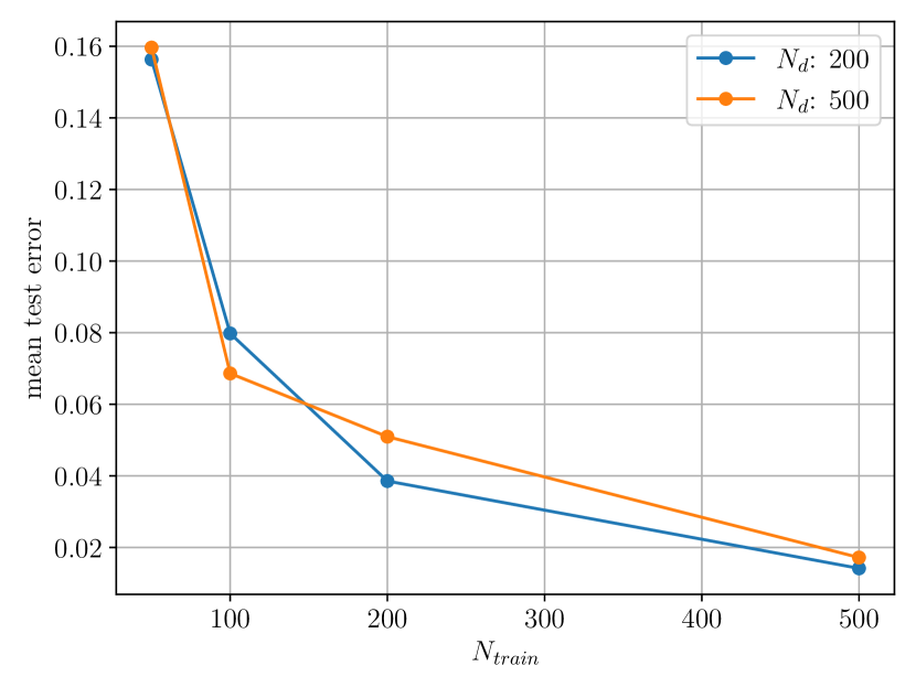
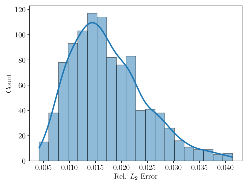
Figure 3: Performance analysis for Reaction diffusion equation: (a) Mean test error over varying $N_{\text{train}}$. (b) Test error distribution of optimal model that achieved an error $0.01742\pm 0.007142$ with $N_{train}=500$, $N_{d}=500$.

Table 2: Reaction Diffusion system: Mean and standard deviation of the test error for all the case with input functions drawn from modified GRFs with varying length-scale parameter, $l$. The experiments were carried out for five independent runs.

$l$	Test Error
0.10	0.1953 $\pm$ 0.1263
0.15	0.09055 $\pm$ 0.07274
0.20	0.04028 $\pm$ 0.03121
0.40	0.01720 $\pm$ 0.01026
0.60	0.01593 $\pm$ 0.01077

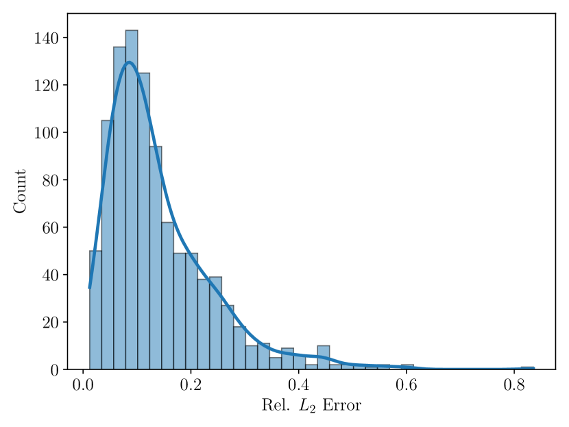
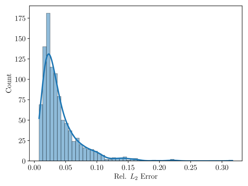
Figure 4: Performance analysis for GRFs and Modified GRFs input function spaces: (a) GRFs basis $l=0.2$, Test error = 0.14039 $\pm$ 0.09857. (b) Modified GRFs basis $l=0.2$, Test error = 0.04028 $\pm$ 0.03121

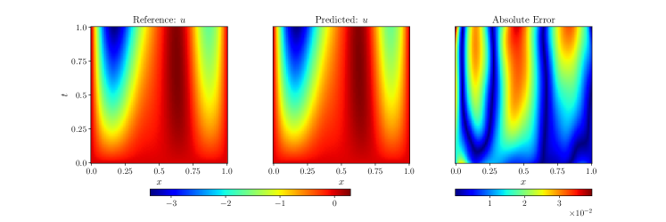
(a) Sample 1: solution field accuracy comparison, relative $L_{2}$ error = 0.01639.

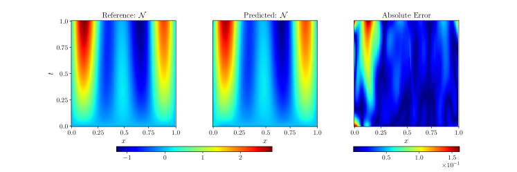
(b) Sample 1: hidden physics solution comparison, relative $L_{2}$ error = 0.03949.

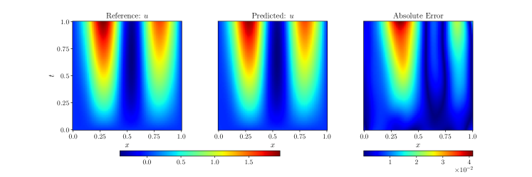
(c) Sample 2: solution field accuracy comparison, relative $L_{2}$ error = 0.01960.

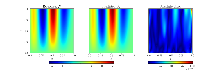
(d) Sample 2: hidden physics solution comparison, relative $L_{2}$ error = 0.02435.

Figure 5: Reaction diffusion equation: Comparison of reference and predicted results for two representative test samples with input function from sine function space.

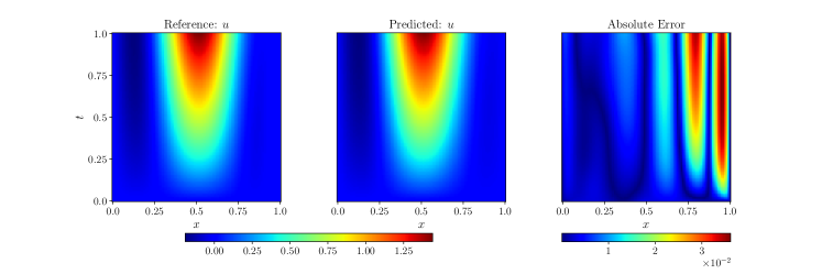
(a) Sample 1: solution field accuracy comparison, relative $L_{2}$ error = 0.02733.

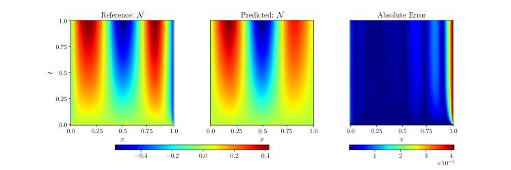
(b) Sample 1: hidden physics solution comparison, relative $L_{2}$ error = 0.34308.

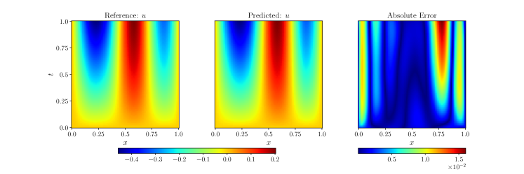
(c) Sample 2: solution field accuracy comparison, relative $L_{2}$ error = 0.0322.

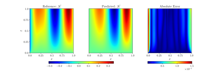
(d) Sample 2: hidden physics solution comparison, relative $L_{2}$ error = 0.23023.

Figure 6: Reaction diffusion equation: Comparison of reference and predicted results for two representative test samples with input function from GRF function space $l=0.2$ (nonzero at boundaries)

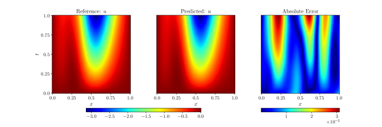
(a) Sample 1: solution field accuracy comparison, relative $L_{2}$ error = 0.01193.

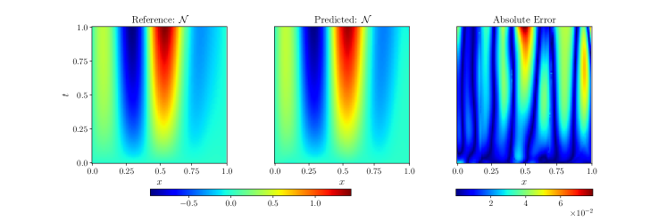
(b) Sample 1: hidden physics solution comparison, relative $L_{2}$ error = 0.05668.

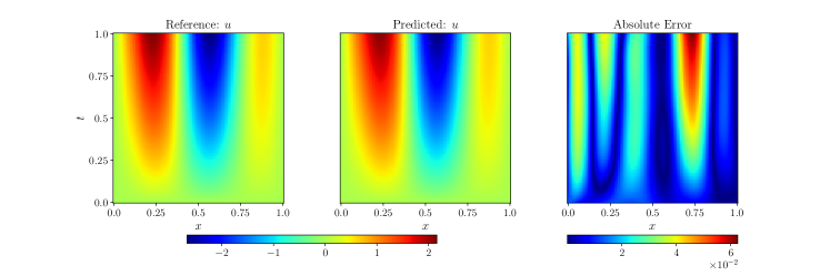
(c) Sample 2: solution field accuracy comparison, relative $L_{2}$ error = 0.02303.

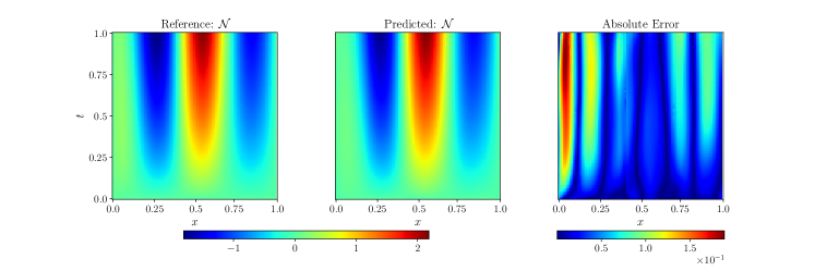
(d) Sample 2: hidden physics solution comparison, relative $L_{2}$ error = 0.07587.

Figure 7: Reaction diffusion equation: Comparison of reference and predicted results for two representative test samples with input function from Modified GRF function space $l=0.2$ (zero at boundaries)

System parameter identification: Diffusion coefficient

The neural operator framework introduced in Section 2.2 is employed to characterize the system, specifically to identify the diffusion coefficient of the governing PDE using solution values at selected spatial and temporal locations.

For this investigation, we considered varying diffusion coefficients and source terms in the Reaction-Diffusion equation defined in Equation 8. The equation was solved numerically using a finite difference method on a uniform grid with spatial resolution $\delta x=0.01$ and time step $\delta t=0.001$, creating a $101\times 101$ grid over the $x$-$t$ domain. The solution dataset was generated using 500 different diffusion coefficient values ($D$) uniformly distributed between $0.01$ and $0.05$. Each diffusion coefficient was paired with 20 distinct source terms $f(x)$ sampled from a Gaussian Random Field (GRF), resulting in 10,000 solution fields. The dataset was split into $N_{\text{train}}=8,500$ samples for training and $N_{\text{test}}=1,500$ samples for testing. To emulate sparse measurements, 300 spatial-temporal locations were randomly sampled and fixed across all training and testing samples, providing known values of $u(x,t)$. The network training hyperparameters are presented in Table 1. The training configuration employs $N_{\text{coll}}=2500$ collocation points for PDE residual evaluation. In the loss function, a penalty coefficient of $\lambda_{\text{coll}}=10$ was applied to the PDE residual term, while unity weights were maintained for data loss terms.

Figure 8 illustrates the framework’s capability in reconstructing the solution field $u(x,t)$ and estimating the diffusion coefficient $D$ from 300 sparse measurements. Results from two representative test cases demonstrate solution reconstruction with $L_{2}$ errors of order $\mathcal{O}(10^{-2})$, along with accurate recovery of the true diffusion coefficient values. Figure 9 presents the distribution of absolute errors in predicted diffusion coefficients across the entire test set, showing that the majority of predictions maintain absolute errors below $0.005$. This indicates the framework’s robust performance in parameter estimation tasks.

It is worth noting that determining the reaction coefficient from this system poses significant challenges due to the nonlinear relationship between $K$ and $u(x,t)$ in the reaction-diffusion equation. Small perturbations in the solution field $u(x,t)$ can lead to substantial errors in the estimation of $K$. Furthermore, the reaction term becomes negligible in regions where $u$ approaches zero, making the inverse problem for $K$ particularly challenging in these regions.

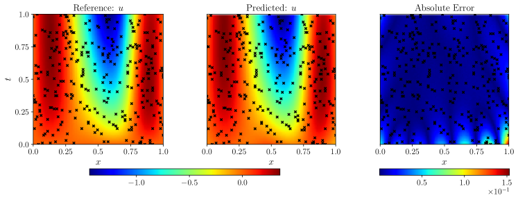
(a) Sample 1: Relative $L_{2}$ error of $u(x,t)$ = $0.027$. For this case, $\nu_{\text{true}}=0.027$ while $\nu_{\text{predicted}}=0.027$.

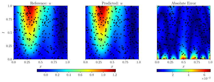
(b) Sample 2: Relative $L_{2}$ error of $u(x,t)$ = $0.029$. For this case, $\nu_{\text{true}}=0.036$ while $\nu_{\text{predicted}}=0.034$.

Figure 8: Reaction Diffusion Equation: Comparison of the reference solution and the predicted solution. The black cross marks represent the location where the data of $u(x,t)$ was known during the testing. The error at these specific locations is also shown in the absolute error plot.

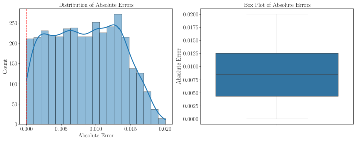
Figure 9: Reaction Diffusion Equation: Distribution of absolute error of $D$ when compared to the $D$ used to generate the ground truth using the finite difference solver. The framework approximates $D$ with a error of $8\times 10^{-3}\pm 0.008$.

3.2 Burgers equation

In this example, we consider the viscous Burgers’ equation defined as:

$$\begin{split}&\frac{\partial u}{\partial t}(x,t)=\nu\frac{\partial^{2}u}{\partial x^{2}}(x,t)-u\frac{\partial u}{\partial x}(x,t)\text{ on }\ \Omega:(x,t)\in[0,1]^{2},\\ \text{IC: }&u(x,0)=f(x),\\ \textnormal{BC: }&u(0,t)=u(1,t)\text{ and }\frac{\partial u}{\partial x}(0,t)=\frac{\partial u}{\partial x}(1,t),\\ \end{split}$$ (13)

where $u(x,t)$ denotes the evolving spatio-temporal velocity field defined using the space and time coordinates, $(x,t)$. In Equation 13, BC denotes periodic boundary condition. Similar to the previous example, we will first present the results of discovering the unknown physics using DeepONet, followed by presenting the results of employing DeepONet to characterize the viscosity of the system using sparse measurements.

Discovering physics using DeepONet

In this problem, we re-write Equation 13 as:

$$\frac{\partial u}{\partial t}(x,t)=\mathcal{N}(u,u_{x},u_{xx}),$$ (14)

where the $\mathcal{N}$ denotes the hidden physics that is a function of the solution field $u(x,t)$ and its spatial derivatives. In this problem, our aim is to learn the solution operator, $\mathcal{G}_{\theta}$ that maps the initial condition, $f(x,0)$ to the solution field, $u(x,t)$ using the partial known physics as well as sparse labeled dataset. In this case, we have considered fixed viscosity for the system, $\nu=0.01$. We solved equation (13) using a finite difference solver on a uniform grid ($\delta x=\delta t=0.01$), resulting in a $101\times 101$ grid spanning the $x$-$t$ domain with initial conditions sampled from a Gaussian Random Field (GRF).

The experiments were conducted with varying numbers of training samples, $N_{train}\in\{50,100,200,500,1000\}$ and the size of labeled dataset, $N_{d}\in\{200,500\}$, where $N_{d}$ denotes the number of locations per sample where the value of solution field is known. For testing, we used a fixed set of $N_{test}=1,000$ samples. Figure 10(a) illustrates the mean test error across different combinations of sample sizes and training data points. The optimal performance was achieved with $N_{train}=1000$ and $N_{d}=500$, resulting in a mean test relative $L_{2}$ error of 0.06140. The loss curve over the training process is shown in Figure 1(b).

The distribution of test errors for this optimal configuration is presented in Figure 10(b). As demonstrated in Figure 11, the model accurately predicts both the solution $u$ and the hidden physics terms when compared to ground truth values. Therefore, the model successfully approximated the unknown hidden term as

$$\mathcal{N}\approx 0.01\frac{\partial^{2}u}{\partial x^{2}}(x,t)-u(x,t)\frac{\partial u}{\partial x}(x,t)$$

.

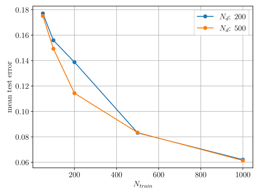
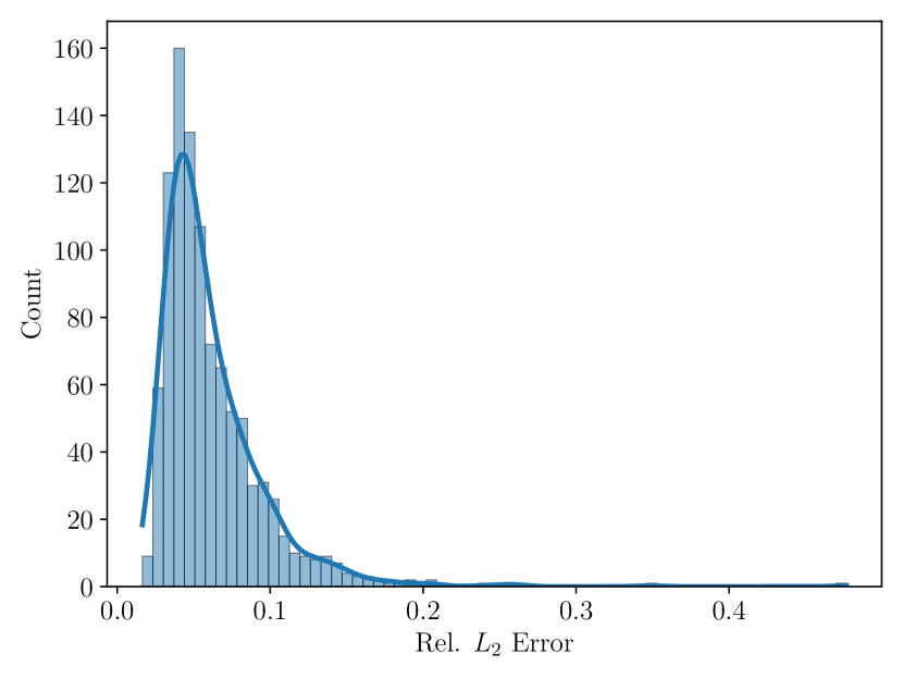
Figure 10: Performance analysis for Burger’s equation: (a) Mean test error over varying $N_{\text{train}}$. (b) Test error distribution of optimal model that achieved an error $0.06140\pm 0.03510$ with $N_{train}=1000$, $N_{d}=500$.

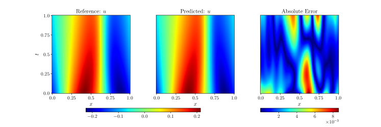
(a) Sample 1: solution field accuracy comparison, relative $L_{2}$ error = 0.02134.

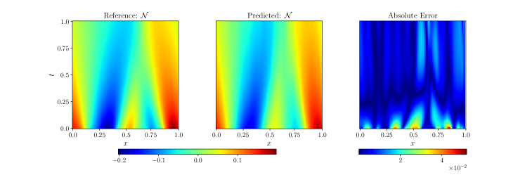
(b) Sample 1: hidden physics solution comparison, relative $L_{2}$ error = 0.118278.

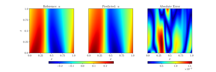
(c) Sample 2: solution field accuracy comparison, relative $L_{2}$ error = 0.03909.

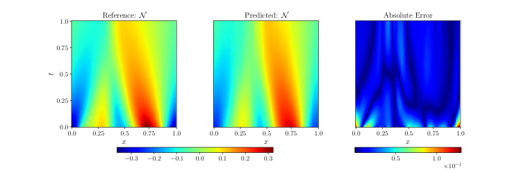
(d) Sample 2: hidden physics solution comparison, relative $L_{2}$ error = 0.15396.

Figure 11: Burgers’ equation: Comparison of reference and predicted results for two representative test samples.

System parameter identification: Viscosity

We are now interested in employing the neural operator framework discussed in Section 2.2 to characterize the system, more specifically to identify the viscosity of the model while being provided with the solution values at a few spatial and temporal locations.

To design the problem, we have considered varying viscosity as well as initial conditions for the Burgers’ equation defined in Equation 13. For data generation, we solved this equation using a finite difference solver on a uniform grid with spatial resolution $\delta x=0.01$ and time step $\delta t=0.01$, resulting in a $101\times 101$ grid spanning the $x$-$t$ domain. The dataset comprises solutions corresponding to 500 different viscosity values ($\nu$) uniformly distributed between $0.01$ and $0.05$. Each viscosity value was paired with 20 distinct initial conditions sampled from a Gaussian Random Field (GRF), yielding a total of 10,000 solution fields. We randomly selected $N_{\text{train}}=8,500$ samples for training and reserved the remaining $N_{\text{test}}=1,500$ for testing the model. To simulate sparse measurements, we randomly sampled 300 spatial-temporal locations (fixed across all training and testing samples) from the solution field, where the value of $u(x^{s},t^{s})$ is known.

The hyperparameters involved in the training of the networks are presented in Table 1. The training configuration utilizes $N_{\text{coll}}=2500$ collocation points for evaluating the PDE residual. The loss functions were weighted with unity penalty coefficients.

Figure 12 demonstrates the framework’s performance in reconstructing both the solution field $u(x,t)$ and estimating the viscosity parameter $\nu$ from $300$ sparse measurements. We present results from two representative test cases selected from our test set of $1,500$ samples. The framework achieves solution reconstruction with $L_{2}$ errors of order $\mathcal{O}(10^{-2})$, while accurately recovering the true viscosity values in both cases. To provide a comprehensive assessment of the parameter estimation accuracy, Figure 13 presents the distribution of absolute errors in predicted viscosity values across the entire test set. The distribution reveals that the majority of predictions exhibit absolute errors below $0.002$, demonstrating the robust performance of our framework in parameter estimation tasks.

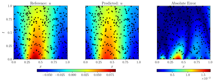
(a) Sample 1: Relative $L_{2}$ error of $u(x,t)$ = $0.092$. For this case, $\nu_{\text{true}}=0.028$ while $\nu_{\text{predicted}}=0.025$.

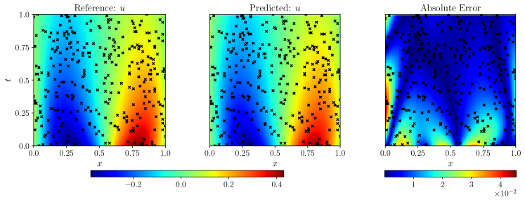
(b) Sample 2: Relative $L_{2}$ error of $u(x,t)$ = $0.061$. For this case, $\nu_{\text{true}}=0.032$ while $\nu_{\text{predicted}}=0.032$.

Figure 12: Burgers’ Equation: Comparison of the reference solution and the predicted solution. The black cross marks represent the location where the data of $u(x,t)$ was known during the testing. The error at these specific locations is also shown in the absolute error plot.

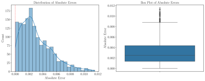
Figure 13: Burgers’ Equation: Distribution of absolute error of $\nu$ when compared to the $\nu$ used to generate the ground truth using the finite difference solver. The framework approximates $\nu$ with a error of $2\times 10^{-3}\pm 0.002$.

4 Conclusion

This study introduces two complementary frameworks that leverage physics-informed operator learning to tackle the challenges of hidden physics discovery and system parameter identification across multiple PDE systems. These frameworks generalize solutions without requiring full knowledge of governing equations, offering a robust approach for both in-distribution and out-of-distribution scenarios. The first framework excels in discovering unknown physics by integrating DeepONet with a multilayer perceptron to learn governing dynamics directly from sparse data, achieving relative $L_{2}$ errors on the order of $\mathcal{O}(10^{-2})$. The second framework focuses on system parameter identification, utilizing a pre-trained DeepONet to initialize a physics-constrained inverse model that estimates parameters with absolute errors on the order of $\mathcal{O}(10^{-3})$. Together, these frameworks qualitatively and quantitatively demonstrate their ability to accurately infer hidden physics and identify governing parameters, even from limited observational data. Although the black-box nature of these models poses challenges in interpreting discovered physics in exact mathematical forms, they efficiently generate finite sets of candidate terms, enabling rapid identification of equations that best fit the observed data. These advancements represent a significant step toward addressing inverse problems in scientific modeling, with applications spanning diverse domains in engineering and the physical sciences.

Author contributions

Conceptualization: VK, DRS, BP, SG
Investigation: VK, DRS
Visualization: VK, DRS
Supervision: BP, SG
Writing—original draft: VK, DRS, BP, SG
Writing—review & editing: VK, DRS, BP, SG

Data and code availability

The code and data that support the findings of this study will be available from the corresponding author on reasonable request upon publication.

Competing interests

The authors declare no competing interest

Appendix A Hyperparameter tuning

In the deep learning community, Weights & Biases (WandB) is a popular online platform that provides tools for monitoring and controlling hyperparameters during model training runs. Sweeps, a crucial component of WandB, allow for the systematic tuning of model hyperparameters. The Sweeps configuration dictionary contains the predefined hyperparameter search space. Depending on this setup, a sweep could include several runs, with grid search, random search, or Bayesian optimization used for hyperparameter sampling. Sarkar et al. [46] showcases the use of WandB for hyperparameter tuning on PINNs training. We have utilized the WandB tool for hyperparameter tuning of our framework for the parameter identification problem of the Burgers equation. The report of the hyperparameter tuning can be found at the link https://api.wandb.ai/links/droysar1-johns-hopkins-university/pzs4hfup.

Table 1: Architecture and training parameters for all the examples presented in this work.

Equation	Branch Network	Trunk Network	MLP or FNN	Activation Function	Training Iterations	Learning Rate (Initial / Decay)	Batch Size
Hidden physics
Reaction-Diffusion	$[101,128,128,128,50]$	$[2,128,128,128,50]$	$[3,128,128,128,1]$	Branch $-$ ReLU Trunk $-$ Tanh MLP $-$ Tanh	10k	$1e-4$	10
Burgers’	$[101,128,128,$ $128,128,50]$	$[2,128,128,$ $128,128,50]$	$[3,256,256,256,1]$	Branch $-$ ReLU Trunk $-$ Tanh MLP $-$ Tanh	10k	$1e-4$	1
System parameter identification
Reaction-Diffusion	$[300,64,64,64,100]$	$[2,64,64,64,100]$	$[300,64,64,64,1]$	Tanh	80k	$1e-3$ exponential, rate = 0.9	$3500$
Burgers’	$[300,64,64,64,100]$	$[2,64,64,64,100]$	$[300,64,64,64,1]$	Tanh	80k	$1e-3$ exponential, rate = 0.9	$2500$

References

- [1] P. Perdikaris, G. E. Karniadakis, Model inversion via multi-fidelity Bayesian optimization: a new paradigm for parameter estimation in haemodynamics, and beyond, Journal of The Royal Society Interface 13 (118) (2016) 20151107.
- [2] B. F. Kennedy, P. Wijesinghe, D. D. Sampson, The emergence of optical elastography in biomedicine, Nature Photonics 11 (4) (2017) 215–221.
- [3] J.-L. Gennisson, T. Deffieux, M. Fink, M. Tanter, Ultrasound elastography: principles and techniques, Diagnostic and interventional imaging 94 (5) (2013) 487–495.
- [4] C.-T. Chen, G. X. Gu, Learning hidden elasticity with deep neural networks, Proceedings of the National Academy of Sciences 118 (31) (2021) e2102721118.
- [5] I. G. Kevrekidis, C. W. Gear, G. Hummer, Equation-free: The computer-aided analysis of complex multiscale systems, AIChE Journal 50 (7) (2004) 1346–1355.
- [6] M. Raissi, Deep Hidden Physics Models: Deep Learning of Nonlinear Partial Differential Equations, Journal of Machine Learning Research 19 (25) (2018) 1–24.
- [7] H. J. Motulsky, L. A. Ransnas, Fitting curves to data using nonlinear regression: a practical and nonmathematical review, The FASEB journal 1 (5) (1987) 365–374.
- [8] C.-W. Chang, M. Ushio, C.-h. Hsieh, Empirical dynamic modeling for beginners, Ecological research 32 (2017) 785–796.
- [9] B. C. Daniels, I. Nemenman, Automated adaptive inference of phenomenological dynamical models, Nature communications 6 (1) (2015) 8133.
- [10] J. Koza, On the programming of computers by means of natural selection, Genetic programming (1992).
- [11] S. L. Brunton, M. Budišić, E. Kaiser, J. N. Kutz, Modern koopman theory for dynamical systems, arXiv preprint arXiv:2102.12086 (2021).
- [12] S. L. Brunton, J. L. Proctor, J. N. Kutz, Discovering governing equations from data by sparse identification of nonlinear dynamical systems, Proceedings of the national academy of sciences 113 (15) (2016) 3932–3937.
- [13] M. Raissi, P. Perdikaris, G. E. Karniadakis, Physics-informed neural networks: A deep learning framework for solving forward and inverse problems involving nonlinear partial differential equations, Journal of Computational physics 378 (2019) 686–707.
- [14] S. Cai, Z. Mao, Z. Wang, M. Yin, G. E. Karniadakis, Physics-informed neural networks (PINNs) for fluid mechanics: a review, Acta Mechanica Sinica 37 (12) (2021).
- [15] W. Wang, T. P. Wong, H. Ruan, S. Goswami, Causality-Respecting Adaptive Refinement for PINNs: Enabling Precise Interface Evolution in Phase Field Modeling, arXiv preprint arXiv:2410.20212 (2024).
- [16] G. Kissas, Y. Yang, E. Hwuang, W. R. Witschey, J. A. Detre, P. Perdikaris, Machine learning in cardiovascular flows modeling: Predicting arterial blood pressure from non-invasive 4D flow MRI data using physics-informed neural networks, Computer Methods in Applied Mechanics and Engineering 358 (2020) 112623.
- [17] M. Raissi, A. Yazdani, G. E. Karniadakis, Hidden fluid mechanics: Learning velocity and pressure fields from flow visualizations, Science 367 (6481) (2020) 1026–1030.
- [18] H. Zhang, H. Wang, Z. Xu, Z. Liu, B. C. Khoo, A physics-informed neural network-based approach to reconstruct the tornado vortices from limited observed data, Journal of Wind Engineering and Industrial Aerodynamics 241 (2023) 105534.
- [19] L. Lu, P. Jin, G. Pang, Z. Zhang, G. E. Karniadakis, Learning nonlinear operators via DeepONet based on the universal approximation theorem of operators, Nature machine intelligence 3 (3) (2021) 218–229.
- [20] S. Goswami, A. Bora, Y. Yu, G. E. Karniadakis, Physics-Informed Neural Operators, arXiv preprint arXiv:2207.05748 (2022).
- [21] Z. Li, N. Kovachki, K. Azizzadenesheli, B. Liu, K. Bhattacharya, A. Stuart, A. Anandkumar, Fourier Neural Operator for Parametric Partial Differential Equations (2021). arXiv:2010.08895.
- [22] T. Tripura, S. Chakraborty, Wavelet Neural Operator for solving parametric partial differential equations in computational mechanics problems, Computer Methods in Applied Mechanics and Engineering 404 (2023) 115783.
- [23] A. Anandkumar, K. Azizzadenesheli, K. Bhattacharya, N. Kovachki, Z. Li, B. Liu, A. Stuart, Neural operator: Graph kernel network for partial differential equations, in: ICLR 2020 Workshop on Integration of Deep Neural Models and Differential Equations, 2020.
- [24] B. Raonic, R. Molinaro, T. Rohner, S. Mishra, E. de Bezenac, Convolutional neural operators, in: ICLR 2023 Workshop on Physics for Machine Learning, 2023.
- [25] Q. Cao, S. Goswami, G. E. Karniadakis, Laplace neural operator for solving differential equations, Nature Machine Intelligence 6 (6) (2024) 631–640.
- [26] T. Ingebrand, A. J. Thorpe, S. Goswami, K. Kumar, U. Topcu, Basis-to-basis operator learning using function encoders, arXiv preprint arXiv:2410.00171 (2024).
- [27] B. Bahmani, S. Goswami, I. G. Kevrekidis, M. D. Shields, A resolution independent neural operator, arXiv preprint arXiv:2407.13010 (2024).
- [28] T. Chen, H. Chen, Universal approximation to nonlinear operators by neural networks with arbitrary activation functions and its application to dynamical systems, IEEE transactions on neural networks 6 (4) (1995) 911–917.
- [29] P. C. Di Leoni, L. Lu, C. Meneveau, G. Karniadakis, T. A. Zaki, DeepONet prediction of linear instability waves in high-speed boundary layers, arXiv preprint arXiv:2105.08697 (2021).
- [30] N. Borrel-Jensen, S. Goswami, A. P. Engsig-Karup, G. E. Karniadakis, C.-H. Jeong, Sound propagation in realistic interactive 3D scenes with parameterized sources using deep neural operators, Proceedings of the National Academy of Sciences 121 (2) (2024) e2312159120.
- [31] K. Kontolati, S. Goswami, M. D. Shields, G. E. Karniadakis, On the influence of over-parameterization in manifold based surrogates and deep neural operators, Journal of Computational Physics (2023) 112008.
- [32] Q. Cao, S. Goswami, G. E. Karniadakis, S. Chakraborty, Deep neural operators can predict the real-time response of floating offshore structures under irregular waves, arXiv preprint arXiv:2302.06667 (2023).
- [33] P. Jin, S. Meng, L. Lu, MIONet: Learning multiple-input operators via tensor product, arXiv preprint arXiv:2202.06137 (2022).
- [34] S. Goswami, D. S. Li, B. V. Rego, M. Latorre, J. D. Humphrey, G. E. Karniadakis, Neural operator learning of heterogeneous mechanobiological insults contributing to aortic aneurysms, Journal of the Royal Society Interface 19 (193) (2022) 20220410.
- [35] E. Zhang, A. Kahana, E. Turkel, R. Ranade, J. Pathak, G. E. Karniadakis, A Hybrid Iterative Numerical Transferable Solver (HINTS) for PDEs Based on Deep Operator Network and Relaxation Methods, arXiv preprint arXiv:2208.13273 (2022).
- [36] A. Kahana, E. Zhang, S. Goswami, G. Karniadakis, R. Ranade, J. Pathak, On the geometry transferability of the hybrid iterative numerical solver for differential equations, Computational Mechanics 72 (3) (2023) 471–484.
- [37] S. Goswami, K. Kontolati, M. D. Shields, G. E. Karniadakis, Deep transfer operator learning for partial differential equations under conditional shift, Nature Machine Intelligence (2022) 1–10.
- [38] S. Wang, H. Wang, P. Perdikaris, Learning the solution operator of parametric partial differential equations with physics-informed DeepONets, Science advances 7 (40) (2021) eabi8605.
- [39] L. Mandl, S. Goswami, L. Lambers, T. Ricken, Separable deeponet: Breaking the curse of dimensionality in physics-informed machine learning, arXiv preprint arXiv:2407.15887 (2024).
- [40] V. Kumar, S. Goswami, K. Kontolati, M. D. Shields, G. E. Karniadakis, Synergistic learning with multi-task deeponet for efficient pde problem solving, arXiv preprint arXiv:2408.02198 (2024).
- [41] S. Karumuri, L. Graham-Brady, S. Goswami, Efficient training of deep neural operator networks via randomized sampling, arXiv preprint arXiv:2409.13280 (2024).
- [42] J. He, S. Koric, D. Abueidda, A. Najafi, I. Jasiuk, Geom-deeponet: A point-cloud-based deep operator network for field predictions on 3d parameterized geometries, Computer Methods in Applied Mechanics and Engineering 429 (2024) 117130.
- [43] K. Kontolati, S. Goswami, G. Em Karniadakis, M. D. Shields, Learning nonlinear operators in latent spaces for real-time predictions of complex dynamics in physical systems, Nature Communications 15 (1) (2024) 5101.
- [44] J. Smoller, Shock waves and reaction diffusion equations, 2nd Edition, Springer Science, Bussiness media LLC, 2012.
- [45] M. D. McKay, R. J. Beckman, W. J. Conover, A Comparison of Three Methods for Selecting Values of Input Variables in the Analysis of Output from a Computer Code, Technometrics 21 (2) (1979) 239–245.
- [46] D. R. Sarkar, C. Annavarapu, P. Roy, Adaptive Interface-Pinns (Adai-Pinns) for Inverse Problems: Determining Material Properties for Heterogeneous Systems, Available at SSRN 4993297.