Robust Computation with Intrinsic Heterogeneity

Abstract

Intrinsic within-type neuronal heterogeneity is a ubiquitous feature of biological systems, with well-documented computational advantages. Recent works in machine learning have incorporated such diversities by optimizing neuronal parameters alongside synaptic connections and demonstrated state-of-the-art performance across common benchmarks. However, this performance gain comes at the cost of significantly higher computational costs, imposed by a larger parameter space. Furthermore, it is unclear how the neuronal parameters, constrained by the biophysics of their surroundings, are globally orchestrated to minimize top-down errors. To address these challenges, we postulate that neurons are intrinsically diverse, and investigate the computational capabilities of such heterogeneous neuronal parameters. Our results show that intrinsic heterogeneity, viewed as a fixed quenched disorder, often substantially improves performance across hundreds of temporal tasks. Notably, smaller but heterogeneous networks outperform larger homogeneous networks, despite consuming less data. We elucidate the underlying mechanisms driving this performance boost and illustrate its applicability to both rate and spiking dynamics. Moreover, our findings demonstrate that heterogeneous networks are highly resilient to severe alterations in their recurrent synaptic hyperparameters, and even recurrent connections removal does not compromise performance. The remarkable effectiveness of heterogeneous networks with small sizes and relaxed connectivity is particularly relevant for the neuromorphic community, which faces challenges due to device-to-device variability. Furthermore, understanding the mechanism of robust computation with heterogeneity also benefits neuroscientists and machine learners.

1 Introduction

The overall dynamical behavior of a neural network is closely related to its parameters. The same network with different parameters exhibits a distinctly different dynamics and hence results in a different computational functionality. Yet, biological networks are highly heterogeneous, with remarkably diverse neuronal and synaptic values. Large-scale studies at various levels [1, 2, 3, 4, 5, 6, 7, 8, 9] have revealed the extent of this variation, which for some parameters can exceed more than two orders of magnitude. How do biological networks function despite such a large breadth of parameter heterogeneity?

To answer this question, many studies incorporated heterogeneity as some form of diverse tuning (disorder), and studied its computational implications. [10, 11, 12, 13, 14] have uncovered that diverse excitability can lead to different firing patterns in neuronal networks. Input gain control has been shown to be possible through external [15, 16] or intrinsic [17] heterogeneities, which respectively result in synchronization and linear or divisive amplification. Within-type heterogeneity has been shown to enhance population coding efficiency [18, 19, 20] and elevate responsiveness [21, 22] in theoretical settings. Moreover, experimental studies have shown that intrinsic within-type heterogeneity enhances information content (by decorrelating neuronal activity) [23] and odor processing [24] in mouse olfactory bulb. Diversities in the granule cells of electric fish [25] and mouse [26] have also been linked to a superior sensory predictive coding. Similarly, efficient coding of natural vocalization in mice is shown to be supported by diverse tuning of inferior colliculus [27]. Yet, despite the wealth of evidence, it is not clear how intrinsic heterogeneity (quenched disorder) manifests itself in solving real-world tasks.

In contrast, recent works in the machine learning community, have demonstrated that optimized heterogeneity (annealed disorder), enhances networks performance in several commonly used benchmarks [28, 29, 30, 31, 32, 33]. Inspired by the experimentally observed heterogeneity, these works treat the neuronal parameters, which traditionally were kept constant and identical across all neurons (or layers), learnable. By virtue of supervised training, the neural parameters thus become diverse, and in some cases, even resemble the experimentally observed heterogeneity profiles. However, despite performances compatible to the state-of-the-art, these models do not provide much understanding regarding the function of biological heterogeneity. The reason is twofold: First, in such models, heterogeneity is merely a mathematical trick to provide an escape route from local minima. Thus, if a good-enough solution can be found without imposing heterogeneity, from a machine learning perspective, there is no reason to incorporate it. Hence, the emerged heterogeneity is solely an artifact of optimization (the annealing process) [30, 31] rather than a biological constraint (quenched disorder). Second, it is not clear how back-propagation and credit assignment problem are solved biologically (although see [34, 35, 36, 37, 38]). This is particularly true for non-synaptic parameters, whose value is controlled by the biophysical constraints of the surrounding environment (neuronal tissue and extracellular matrix). Furthermore, due to the expansion of optimization space, models that optimize for heterogeneity suffer from the curse of dimensionality, and thus are computationally very demanding (as also noted in [30, 33]). This is in odds with biology, where biological brains, despite having orders of magnitude more parameters than the current largest artificial models, still support learning and behaving with much less power consumption. Therefore, while such machine learning studies effectively demonstrate the benefit of heterogeneity in real world problems, they drastically depart from the path the biology has taken.

To fill this gap, we construct intrinsically heterogeneous networks (similar to earlier works). But instead of studying their dynamical properties, we directly benchmark them against a large variety of “real-world” tasks. The impact of heterogeneity is then assessed by comparing the overall performance of networks, with various levels of heterogeneity, across all such tasks. We use the reservoir computing (RC) paradigm –due to its similarity to neural processing in prefrontal cortex– and construct a family of temporal tasks that mimic working-memory-related computations. Importantly, we design our task family with two goals in mind: comprehensiveness and the guaranteed failure. While the former allows us to judge the effect of heterogeneity in a more task-unbiased manner, the latter, ensures that networks can be well discerned from one another, because the tasks are complex to guarantee that all networks eventually fail. This task design distinguishes this work from works such as [30, 14], where the benefit of heterogeneity is demonstrated only for a handful of tasks, with some being overly simple (periodic functions). Moreover, to gain understanding, we deliberately use the simplest neural dynamic (i.e., leaky-integrator neuron) to minimize complications that might arise in more complex models, e.g., the ones proposed [32, 33] (such as opposing effects of multiple parameters).

Our results suggest that intrinsic (quenched) heterogeneity, even without supervised optimization (annealing), elevates the overall performance across a wide range of temporal tasks. This is due to enrichment of network’s dynamical state that facilitates function approximation capacity and lowers classification latency by faster separation of dissimilar inputs. In particular, we extend the robustness results reported in [30] to a larger task family, and network parameters. Moreover, we empirically show that heterogeneity-induced state enrichment is largely insensitive to the choice of neuronal dynamic, in the sense that both rate and spiking networks show similar enhancement trend. Thus, intrinsic heterogeneity can be utilized in both deep learning and neuromorphic computing. Furthermore, we show in heterogeneous networks synaptic connections play an insignificant role in task execution, and their complete removal does not reduce the overall accuracy, which can be potentially exploited in hardware design as it removes the need for distributed wiring. In summary, this study provides a firm evidence for the functional role of intrinsic biological heterogeneity (quenched disorder), even without top-down optimization.

2 Results

We construct several networks, distinguished by their level of heterogeneity in their neuronal membrane time constant, $\tau_{i}$. In a homogeneous network, which serves as control, all neurons share the same time constant $\tau_{i}=\tau_{0}$, whereas time constants of neurons in other networks are dispersed according to log-normal distributions with the same mean, $\operatorname{\mathbb{E}}[\tau]=\tau_{0}$, but distinct variances. We used variance levels $\operatorname{\mathbb{V}ar}[\tau]=\{\tau_{0}/10,\tau_{0},10\tau_{0},100\tau_{0}\}$, which we refer to, respectively, as low, medium, high and very high heterogeneity. $\tau_{0}$ is (some estimated) characteristic timescale of the stimulus $\bm{u}(t)\in\mathbb{R}^{K}$, serving as a base timescale that ensures all networks operate on the correct temporal range – networks with much faster or much slower neurons either fail to maintain the input’s memory or miss its fluctuation. Other than the time constants, all other conditions are identical across different networks (connectivity matrix, input weights, noise realization, and initial conditions).

Every network is composed of $N$ inhibitory and excitatory neurons in loose balance [39, 40] that are connected together randomly and sparsely (with connection probability $p$) according to Dale’s law. A fraction $f$ of the neurons are excitatory. A dense feedforward projection maps the multi-modal stimulus $\bm{u}(t)\in\mathbb{R}^{K}$ to all neurons. The feedforward weights are drawn from a normal distribution, so that (on average) no net inhibition or excitation is exerted on each neuron. Recurrent and feedforward weights are suitably scaled to ensure that the variance of the corresponding input is independence from the network size $N$ or input dimensionality $K$. Furthermore, a global gain $J$ is applied to the recurrent connections to ensure that all networks operate in the input-driven regime (as opposed to state-driven autonomous regime). Moreover, Each neuron receives an additive i.i.d. white noise with a variance equal to 10% of that of the stimulus.

Both leaky-integrator (rate-) and leaky-integrator and fire (spike-based) dynamics are considered. In either case, the membrane voltage of all networks is integrated via forward Euler method and the same time step $\Delta t=\ll\min_{\{}\tau\}$ (where minimum runs over all networks). Network state, $X(t)$, is constructed by passing the voltages (of rate neurons) through a sigmoidal nonlinearity and convolving the spikes trains (of spiking neurons) with a causal exponential kernel. A windowed subset of $X(t)$ (training set) is used to linearly approximate some arbitrary target function $y(t)$, while the remaining interval (test set) is used to measure the generalizability of the estimated linear decoder, $\bm{\beta}\in\mathbb{R}^{N+1}$ (intercept included). Performance is quantified on the test set by the coefficient of determination, a normalized scalar score $s\in(\infty,1)$ that determines how close the network prediction, $\hat{y}=\bm{\beta}\cdot X$ is to the ground truth $y$, with 1 denoting a perfect match and 0 being the chance level. For visualization purposes, however, we monotonically transform this score, via $s^{\prime}=exp(s-1)$, to the (0, 1) range. This helps us to spot all cases where heterogeneity moves the performance above or below chance level.

In this work, the tasks $y$ are limited to a generic form of working-memory computation, an input-output mapping $y(t)=\mathcal{F}_{\theta}[\bm{u}(t)]$, characterized by the family $\mathcal{F}_{\theta}$ and task parameters $\theta$. In particular, to incorporate a wide range of behaviorally pertinent tasks we consider $y(t)=\mathcal{F}_{\theta}[\bm{u}(t)]=u_{k}(t+\Delta)^{d}$, where the parameters $\theta=(k,\Delta,d)$ respectively select the input modality to be extracted (mirroring signal extraction), control the temporal shift to the past (memory recall) or future (prediction), and determine the extent of nonlinearity applied to the time-shifted stimulus (non-linear input processing). In working memory tasks, task complexity, in addition to the functional form of the family $\mathcal{F}$, also relates to the specifics of the stimulus. In reality, different sensory modalities have different temporal characteristics, and moreover, are only partially predictable. Therefore, to replicate these “real-world” conditions, we feed all networks with a multi-dimensional chaotic stimulus. The chaotic nature of our stimulus, in conjunction with the functional form of $\mathcal{F}$, ensures that our task is complex enough to guarantee failure, which is necessary to discern networks from one another. As such, chaotic timeseries processing, serves as an ideal benchmark to assess the computational capacities of dynamical systems like multi-timescale recurrent networks.

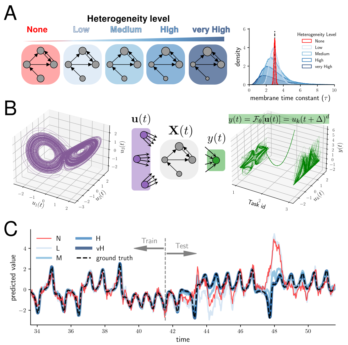
Figure 1: Method summary. (A) Several topologically identical recurrent networks are constructed, which differ only in their neuronal time constant variance. The homogeneous network contains identical neurons (and the small dispersion in the corresponding distribution on the right is visualization possesses only). (B). The same multi-dimensional chaotic timeseries, resembling multimodal, partially predictable sensory stimuli, derives all networks (left). The resultant state, $X(t)$ (middle), is then used to linearly approximate a family of tasks $\mathcal{F}_{\theta}$, that mimic working-memory-related computation (memory recall, forecasting, and nonlinear processing). A few of such tasks are plotted on the right. (C) The approximation accuracy of each network is quantified by the coefficient of determination on the test interval, which measures the (normalized) mismatch between the ground truth and the predicted value.

2.1 Nonlinear processing of chaotic timeseries

In our first experiment, we constructed networks of $N=1000$ neurons, with E/I ratio 4:1 and connection probability $p=0.1$. Networks were driven by the solution of Lorenz systems (c.f. section 6.4), which is a well-known 3-dimensional chaotic timeseries. The stimulus, after component-wise standardization, was densely projected to all neurons in the network, resulting in a time-dependent state $X(t)$. Subsequently, we used the state of each network to decode 465 tasks corresponding to distinct parameters within the range $k=\{1,2,3\},d=\{1,...,5\}$, and $\Delta=[-2\tau_{0},2\tau_{0}]$ (c.f. figure 2A). A summary of performance is depicted in figure 2B-D.

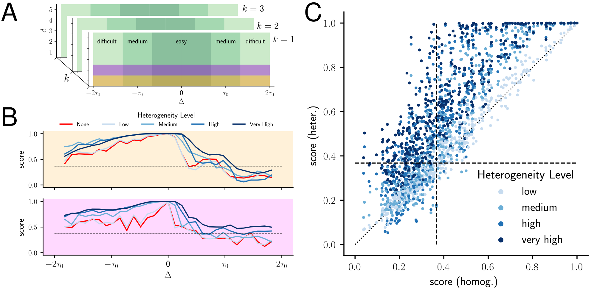
Figure 2: Intrinsically heterogeneous networks process chaotic timeseries more accurately than homogeneous ones. (A) The schematic of our task space. The highlighted orange and magenta bands on the frontal slice correspond to panels (B) and (C), respectively. (B) Score profile of different networks for linear ($d=1$) processing of first input component ($k=1$) for various temporal shifts ($\Delta$). More heterogeneous networks outperform the homogeneous networks for nearly all shifts. All scores are exponentially transformed into the (0,1) range before visualization. The dashed line at $\approx 0.4$ delineates the chance-level score. (C) Same as (B) but for a nonlinear processing ($d=2$) of the same component. (D) Score comparison between the homogeneous (x-axis) and multiple heterogeneous (y-axis) networks, for all tasks. Each distinct task parametrization $\theta=(k,\Delta,d)$ corresponds to one dot. Colors indicate the level of networks’ heterogeneity. The diagonal, dotted line, indicates equal performance. For the majority of tasks, heterogeneous networks outperform the homogeneous ones.

Figures 2B and C depict the decoding score profiles of different networks for, respectively, linear ($d=1$) and nonlinear (quadratic, $d=2$) processing of first input component ($k=1$) and various temporal shifts, $\Delta$. For nearly all values of $\Delta$, the more heterogeneous networks outperform the homogeneous control, suggesting the benefit of heterogeneity for the temporal task processing. However, such superiority may have been biased by our choice of $(k,\Delta,d)$. Thus, to reduce such bias and gain a more holistic view, in figure 2C we visualized the scores of heterogeneous networks against their homogeneous analog for all tasks, as a scatter plot. Every dot in this figure represents a distinct task parameter $(k,\Delta,d)$, while the colors indicate networks’ heterogeneity level. For the majority of tasks (dots), scores lie above the identity line, with some squashed to the perfect score of 1. This, implies that, overall, nonlinear processing can be more accurately performed via heterogeneous networks.

Note that, as figures 2D and A.1D show, not all tasks profit from a higher diversity. This indicates that whether biological heterogeneity is beneficial, as expected, is highly task-dependent. Therefore, benchmarking networks against only a handful of tasks must be avoided, due to its potentially high bias. Instead, a more pragmatic approach is to constrain ourselves to a certain class of tasks (e.g., working-memory, navigation, decision-making, motor movement, etc.), and investigate if a particular biological feature (like intrinsic heterogeneity) overall provides any computational leverage. For instance, here, although we cannot claim that heterogeneity is always advantages, we can argue that, overall, it enhances function approximation capabilities for temporal tasks.

We also tested for chaotic inputs, which, unlike the Lorenzian stimulus, have dynamically independent components. However, we observed no qualitative difference (c.f. supplementary section A). Therefore, in the following sections, we only focus on the Lorenzian stimulus.

2.2 Enhancing computation by repertoire enrichment

Why does neuronal heterogeneity, despite not being tuned to any of members of $\mathcal{F}$, elevates performance for a large fraction of tasks? Note that, for a specific network, the state $X(t)$ is being used to decode multiple tasks. Thus, if a network performs overly better or worse than the other, the fundamental difference lies under their distinct dynamical structure (or repertoire).

It is long-known that a linear readout of any dynamical system, has a bounded information processing capacity, which is controlled by the rank of the (observable) dynamical state $X$ (or the activity matrix) [41, 42]. A system with high redundancy in its activity (low-rank), can only generate a few (linearly) independent temporal modes, whereas a complex activity (high-rank) can support several. Thus, one might expect that, networks with a higher neuronal diversity, encode their input into a more diverse dynamical repertoire. To assess this hypothesis, we computed the relative prominence of (linearly) independent modes of different network through singular value decomposition. As expected, figure 3 shows that more diverse networks exhibit a flatter singular value profile, indicating the more similar contribution of modes in the overall activity. Simply put, the state of more heterogeneous networks is more high-dimensional, which is synonymous with a more enriched dynamical repertoire.

This implies that independent of the underlying dynamic, as long as the network maintains a diverse set of input traces, that support formation of a richer dynamical repertoire, higher function approximation capability can be achieved. Thus, in principle, heterogeneity can be exploited by a wide range of physical reservoirs, including a spiking one, which underpins communications in biological brains. Hence, to assert this conjecture, we adapted our neuronal dynamics from rate to spike, while keeping all network and time constants configurations intact. As shown in the supplementary section B, we indeed observed a very similar behavior, with heterogeneous networks generally outperform their homogeneous counterparts. Thus, heterogeneity-induced enrichment offers an opportunity for neuromorphic chip manufacturers to first, utilize the intrinsic heterogeneity, and second, to explore other “neuronal architectures” in their devices.

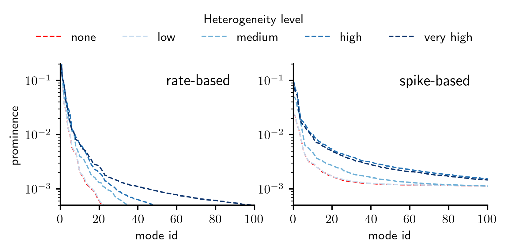
Figure 3: Heterogeneity enriches the dynamical state In both rate- (left) and spike-based dynamics (right) higher heterogeneity enlarges the prominence of (linearly) independent modes, resulting in a repertoire with higher dimensionality. Prominence is defined as the ratio between each singular value to their sum.

2.3 Robustness to hyperparameters

Does the benefit of heterogeneity vanish if we use another set of hyperparameters? To answer this question, we altered all our hyperparameters, namely the mean neuronal time constant $\operatorname{\mathbb{E}}[\tau]$, global recurrent gain $J$, network size $N$, fraction of excitatory neurons $f$, sparsity $p$, and populations weight dispersion $\sigma_{0}$ (which progressively relaxes Dale’s law). As before, for each configuration, a series of networks with different heterogeneity levels were generated, and for each network, the decoding scores of all members of the task family $\mathcal{F}$ were quantified. For brevity, here we only discuss the sensitivity to $\operatorname{\mathbb{E}}[\tau],J$, and $N$. The effect of variation of other parameters (or spiking dynamics) are presented in the supplementary C. Unless otherwise stated, a network of size $N=250$ is used.

Figure 4: More heterogeneous networks outperform independent of the average network time constant. The letter-value plots representing the distribution of all 465 tasks in family $\mathcal{F}$, broken down into three complexity tiers, delineated by the background color matching the categories defined in figure 2A: easy (top), medium (middle) and difficult (bottom). In all panels, heterogeneity either elevates the performance of the bulk of tasks or leaves it nearly intact.

We start by allowing the average time constant $\operatorname{\mathbb{E}}[\tau]$ to take values (half an order of magnitude) smaller or greater than the base timescale $\tau_{0}$. The subsequent networks are collectively referred to as fast and slow, due to their input integration rate in relation to the medium networks with $\operatorname{\mathbb{E}}[\tau]=\tau_{0}$. As before, for all average levels, the linear decoding score for tasks in $\mathcal{F}$ is quantified. Figure 4 shows a breakdown of such score distribution by $\operatorname{\mathbb{E}}[\tau]$, heterogeneity, and task complexity tier (which is largely dominated by the shift values $|\Delta|$). Also, look at figure C.2 for the spiking equivalent.

For nearly all complexity tiers, more heterogeneous networks exhibit better performance. However, there is a systematic score gradient across $E[\tau]$, with faster networks outperforming slower ones. This gradient is largely due to the fast autocorrelation decay of our target functions (inherited from the one of the Lorenzian timeseries). In general, for a faithful representation, autocorrelation of the state $X(t)$ must be similar to that of the target. While, fast network with only short memory are suitable to represent rapidly changing inputs, targets with long-term (temporal) dependencies can be represented accurately only if the networks preserves such long-term input traces. In reality, however, the rate of input fluctuations is unknown, a priori. Hence, having multiple timescales is a simple strategy to ensure that for any arbitrary set of temporal timescales in the input, some neurons are capable to tune in, with good-enough accuracy. This can be most easily observed, for instance, in figure 4A3, where higher heterogeneity increases the fraction of fast neurons –what needed to better tune to the fast input–, which indeed results in higher performance.

Yet, the above argument holds only input-driven reservoirs, in which the initial state gradually fades away, leading to a state that follows the input. Consequently, this operational regime (also known as fading-memory property [43, 44], echo-state property [45], or more generally contractive [46] or dissipative dynamics [47]) is best to form input-output associations. In contrast, in autonomous or state-driven regime, the strong synaptic ties between neurons can maintain (or even amplify) the initial state, giving raise to either attractors [48, 49] or chaotic orbits [50, 51, 52] that are very sensitive to the initial state, as well as noise.

Therefore, a natural question is how well homogeneous and heterogeneous networks perform when initialized close to or in the autonomous regime. To answer this question, we altered the recurrent gain $J$ from its nominal value of 1– representing the case where the endogenous (recurrent) and exogenous (feedforward) equally influence a typical neuron– to more input-driven ($J<1$) or state-driven ($J>1$) conditions. Figure 5 (c.f. C.2 for spiking dynamic) summarizes the decoding score distribution breakdown as $J$ is varied.

Figure 5: Heterogeneous network are resilient against synaptic gain change. As in figure 4 but for various levels of synaptic gain $J$. $J=1$ marks the configuration where the endogenous and exogenous inputs equally influence a typical neuron. $J>1$ is biased towards autonomy. Note that even for $J=0$, which is equivalent to removing all recurrent connections, heterogeneous networks maintain their high performance.

Figure 5 shows that, as expected, the overall performance of networks progressively decreases as $J$ increases. Moreover, this rate is the fastest for homogeneous networks (whose performance quickly drops to below chance-level), and slowest for highly heterogeneous networks, which consistently perform well in nearly all values of synaptic gains. A particularly interesting observation is the effectiveness of a heterogeneous network with zero synaptic gain. This case corresponds to an ensemble of isolated neurons that integrate the input without communication, effectively forming a filter bank. As figure 5 illustrates, such ensembles, if heterogeneous enough, are capable of forming a rich state that performs as well as interconnected systems. This indicates that, for certain tasks (like those temporal tasks represented in the family $\mathcal{F}$), the synaptic interconnection is not vital, and computation can be carried out by ensuring the diversity of neurons alone. In other words, it is possible to remove all synaptic connections, without compromising the performance. This is particularly useful for analog or neuromorphic device manufacturers, since it indicates that simpler devices, with minimal internal wiring (thus lower fabrication cost), are as effective.

Figure 6: Heterogeneity helps robust and fast learning in small size. As in figure 4 but for various system size. The training window is expanded proportional to the size of each network so that the number of samples per parameter stays the same. All networks are evaluated on a test interval of the same size. Smaller heterogeneous networks, despite having fewer training samples, perform as well as much larger homogeneous ones in all complexity tiers.

We next investigated the effect of system size and summarized the results in figure 6. As expected, larger system size enhances performance across all tasks complexities and all heterogeneity levels. However, the performance gap between heterogeneous and homogeneous networks is never filled. Although for a large enough system this disparity might vanish, such up-scaling is unnecessary. For instance, as figure 6 illustrates, a small ($N=100$) but highly heterogeneous network performs equally (or even better) than a much larger ($N=1000$) but entirely homogeneous network, even though the heterogeneous system is one order of magnitude smaller, and is trained with 10 times fewer samples (while evaluated on the same test set). Thus, it seems clear that utilizing heterogeneity is not only enhances performance, but also is an effective strategy to do so with minimal resources and shorter training.

3 The importance of outliers

We conclude the results by remarking that not all heterogeneity profiles are equivalent. While we used log-normal distribution to sample time constants in the previous sections, using a normal or uniform distributions with identical empirical statistics (mean and variance) do not result in any performance boost. On the contrary, sampling from gamma, another long-tail distribution, does display similar score enhancement (c.f figure C.1A). The commonality between gamma and log-normal profiles is that they both can give raise to “outlier” neurons, i.e., those with time constants much larger than the mass of neurons. Hence, our results suggest that outliers are vital for accurate temporal processing. This is congruent with observations in both experimental [7] and artificial [30] system, that also report highly skewed time constant profiles.

4 Discussion

Real neurons are highly heterogeneous. Inspired by this neuron specificity, recent works in machine learning treated neuronal parameters trainable and showed state-of-the art performances across a series of conventional benchmarks. These works, however, heavily rely on supervised back-propagation, which, apart from their susceptibility to catastrophic forgetting, do not answer how credit assignment problem is solved biophysically, what is the function of the intrinsic heterogeneity, and how does the brain overcome the curse of dimensionality.

In this work, we diverged from this approach by postulating that biological organisms do not optimize (anneal) heterogeneity in their lifetime, but rather function on top of this intrinsic (quenched) diversity, which may have formed during evolution. Hence, we aimed to investigate whether or not such intrinsic heterogeneity have any utility for robust computation. While this problem has been posed previously (c.f [30, 14]), to the best of our knowledge, it has never been demonstrated if intrinsic heterogeneity is of utility for large classes of tasks. In this work, we addressed this gap by constructing a comprehensive and complex task family encompasses working-memory-related computations, and showed that heterogeneity is generally but not always beneficial in temporal sensory processing. Moreover, we showed that the robustness of heterogeneous networks to hyperparameters goes far beyond the ones previously reported in [30].

In particular, by considering hundreds of distinct tasks, we found that small but heterogeneous networks perform equally well or better than a homogeneous network 10 times larger trained on 10 times more data (c.f. figure 6). Moreover, performance of heterogeneous networks was the least sensitive to the recurrent connectivity, to the extent that removing all connections did not alter performance distribution, despite effectively transforming the network topology to a simple filter bank (c.f. figure 5). These results, alongside its applicability to spiking dynamics (c.f. section B), constitute heterogeneity of substantial relevance for the neuromorphic community. Chip manufacturers constantly face the inevitable device-to-device variability (intrinsic heterogeneity), the challenge of fabricating complex wiring across units (arbitrary connectivity), and ensuring high performance despite few resources (small size). This work demonstrates that by embracing such unavoidable variability, it is possible to reach higher performances in small sized network, and simultaneously reduce the fabrication complexity due to insignificance of recurrent connection.

The intuition behind the observed performance boost is as follows. Each neuron in a typical (input-driven) reservoir maintains some history of its input, which ultimately depends on its tuning. In a homogeneous reservoir, all neurons tune to the input similarly, forming a dynamical repertoire that is more or less redundant. In contrast, in heterogeneous reservoirs, the input is embedded in a more diverse set of neural traces, forming a relatively richer dynamical repertoire that can approximate more intricate target functions. While one can also promote this richness by altering connectivity (i.e., synaptic properties), in this work enrichment was predominantly neuronal, since for a fixed (non-zero) heterogeneity level, removing all recurrent connections (c.f. figure 5), changing sparsity or altering E/I ratio (c.f. figure C.1B and C) did not lead to systematic change in the score distribution.

We also noticed that the success of heterogeneous networks to outperform temporal tasks is intimately related to the existence of a few “outlier” neurons that enable networks to preserve long-term input fluctuations (c.f. section 3 and figure C.1A). A heterogeneity profile, devoid of such outliers, does not yield any noticeable performance gain over homogeneous systems. Interestingly, supervised training of reservoirs on entirely different temporal tasks also gives raise to skewed distribution [30], suggesting that long-tail distribution are somehow related to the generic structure of temporal tasks, rather than specifics of each task or training process. However, it is not clear why that is the case, or whether such skewed distribution are universally optimal, i.e., for all temporal tasks, and/or other classes of tasks (decision-making, motor control, navigation, etc.). Further theoretical investigations are needed to answer these questions.

From a practical point of view, incorporating heterogeneity in a model necessitates answering one key question: For a given computation, diversity of which parameter matters the most? Indeed, The task family we devised was anchored to working-memory-like computations, which (by definition) unfolds in time. Consequently, it is not hard to guess that temporal parameters play a crucial role (also look at [32] who showed that optimizing synaptic delays and neuronal time constants – both temporal parameters – have similar effects in solving temporal tasks). Yet, if the desired computation entail, e.g., spatial or hierarchical structures, a heterogeneous tuning supporting such spatial or hierarchical structure is likely to be more integral to task execution than, for instance, diverse time constants. A classic example in this regard is the diversity of orientation selective cells in mammalian visual cortex [53, 54]: Animals are able to identify all orientations because V1 cells support such diverse representation. The main takeaway is that the diverse parameter should, in some sense, suit the type of task at hand. Hence, identifying the correct parameter requires as much understanding of the underlying biology as of the task type itself.

While we only considered regression in this work, the aforementioned intuition can be readily generalized to other computational problems. For instance, our preliminary work suggests that heterogeneous networks classify inputs faster than homogeneous ones (data not shown). In a reinforcement learning setting, experiments support the possibility of flexible prioritization between long- and short-term task demands through reward traces of different timescales [55]. Given the well-documented hierarchical structural of timescales in the brain [56, 57], it is not unlikely that the brain uses a similar principle for various forms of computations.

Although here we mainly focused on input-driven reservoirs, autonomous systems have been also proposed to be play a role in neural computation. For instance, attractor dynamics with invariant sets are linked to long-term memory [58, 48], autonomous periodic patterns are suggested to act as an internal clock [59, 60], and general transient behavior-specific sequences (such as those observed in [61, 62, 63]) have suggested serving as a backbone for generating other sequential activities [64, 65]. While it is not difficult to envision how heterogeneity can potentially enhance computations in these cases (e.g., increasing attractors’ capacity by reducing memory overlaps, constructing a spectrum of internal clocks, and tunable sequence generation), this is not the case for the other class of autonomous which entails irregular and chaotic activity. Despite being identified for long time [66, 67], and even mechanistic models that explain emergence of such chaotic activity [39, 40], the computational advantage of such irregular patterns is not very well know. Consequently, it is not clear how parameter heterogeneity can be of use in such chaotic state-driven systems.

5 Conclusion

In this work, we demonstrated that intrinsic (quenched) neuronal heterogeneity, even without top-down optimization, can substantially enhance networks’ performance and its resilience to hyperparameter mistuning. Embracing this often-neglected biological feature provides valuable insights into how the brain functions with diverse resources, and also opens a potent avenue to engineer more efficient neuromorphic devices.

6 Method

6.1 Reservoir Setup

Each network (reservoir) is composed of $N$ rate-based leaky integrator neurons, with a fraction $f$ being excitatory (E) and the remaining $1-f$ inhibitory (I). As in reservoir computing (RC) framework, neurons are connected randomly yet sparsely with connection probability $p$. Note that the synaptic in-degree is not fixed. Thus, some neurons may have slightly more or slightly fewer synapses than the expected value $Np$. The element $w_{ij}$ of the (sparse) recurrent weight matrix $W\in\mathbb{R}^{N\times N}$ delineates the synaptic weight from neuron $j$ to $i$, and is drawn from a population-specific Gaussian distribution with mean and variance $\mu_{x},\sigma^{2}_{x}$ ($x\in\{I,E\}$). We assumed that afferent inputs to each neuron were balanced, i.e.: $f\mu_{E}+(1-f)\mu_{I}=0$, and both populations had the same synaptic weight dispersion $\sigma^{2}$. Note that the sign of $w_{ij}$ determines if it is excitatory or inhibitory. Thus, $\sigma^{2}$ can be thought as a parameter that gradually relaxes Dale’s law (c.f. figure 7). Unlike [68], we did not impose the tight-balance condition, as it seems too strict to be true in biological settings. The feed-forward weights $W^{u}\in\mathbb{R}^{N\times K}$ are densely initialized with values drawn from a standard normal distribution $\mathcal{N}(0,1)$. To ensure that the variance of recurrent and feedforward inputs are independent of the number of afferents, recurrent and feedforward projections are scaled by $1/\sqrt{Np}$ and $1/\sqrt{K}$.

Figure 7: Weight dispersion relaxes Dale’s law Connectivity matrix (top) and the weight distribution for networks with weight dispersion of (A) $\sigma=1$ and (B) $\sigma=5$.

The membrane voltage of neuron $i$, $v_{i}$, evolves according to leaky-integrator dynamic:

$$\tau_{i}\frac{dv_{i}(t)}{dt}=-v_{i}(t)+\frac{J}{\sqrt{Np}}\sum_{j=1}^{N}w_{ij}r(v_{j}(t))+\frac{J_{u}}{\sqrt{K}}\sum_{k=1}^{K}w^{u}_{ik}{u_{k}}(t)+D\sqrt{\Delta t}\xi_{i}(t)$$ (1)

in which $\tau_{i}$ is the (neuron-specific) integration time constant, $\sigma(.)$ is a static non-linearity (not to be mistaken by the weight dispersion), $u_{k}(t)$ denotes the $k$th component of the feedforward stimulus, $\xi_{i}(t)\sim\mathcal{N}(0,1)$ is the neuron-specific white noise whose strength is controlled by diffusion factor $D$, and $J$ and $J_{u}$ are respectively the global recurrent and feedforward gains that shift the reservoir toward input- or state-driven regimes. Throughout this work we used $J_{u}=1$ and (positive only) sigmoidal activation function

$$r(x)=[1+\exp(-x)]^{-1}$$ (2)

Unless otherwise stated, we set $J=1$, where neither recurrent and feedforward inputs dominates the other. Furthermore, we set $D=0.1$, which is analogous to a signal-to-noise ratio of 10, since the stimulus is standardized (c.f. subsequent section).

The dynamic of spiking neurons is similar. We employed the leaky-integrator and fire dynamic:

$$C_{i}\frac{dv_{i}(t)}{dt} =g(E-v_{i}(t))+I_{0}{I}_{bg}+I_{0}\Big{[}\frac{J}{\sqrt{Np}}\sum_{j=1}^{N}w_{ij}\kappa(t)*s_{j}(t)+\frac{J_{u}}{\sqrt{K}}\sum_{k=1}^{K}w^{u}_{ik}{u_{k}}(t)+D\sqrt{\Delta t}\xi_{i}(t)\Big{]}$$

or equivalently

$$\tau_{i}\frac{dv_{i}(t)}{dt} =-v_{i}(t)+(E+I_{0}I_{bg}/g)+I_{0}/g\Big{[}\frac{J}{\sqrt{Np}}\sum_{j=1}^{N}w_{ij}\kappa(t)*s_{j}(t)+\frac{J_{u}}{\sqrt{K}}\sum_{k=1}^{K}w^{u}_{ik}{u_{k}}(t)+D\sqrt{\Delta t}\xi_{i}(t)\Big{]}$$ (3)

with neuron-specific capacitance $C_{i}$, input conductance $g$, and the reversal potential $E$, whose effect is canceled by introducing a constant background current $I_{bg}$. For convenience, we introduced the unitful quantity $I_{0}$, that allows us to use unitless quantities in the square bracket. The neuron specific membrane time constant is defined as $\tau_{i}=C_{i}/g$. All quantities match their rate-based analog. In particular, similar to equation 1, the stimulus is feed to the neurons as (unitless) continuous current (as opposed to spike). The main difference between the two formulations is the presynaptic spike train $s_{j}(t)=\sum_{t^{f}_{j}}\delta(t-t^{f}_{j})$ (firings at times $t_{f}^{j}$) and the postsynaptic potential (PSP) kernel $\kappa(t)$, as opposed to the nonlinearity $r(.)$. We implemented several PSP kernels, including delta, exponential, and alpha. Yet, we observed no qualitative difference between the generated spike trains. Thus, we ultimately used the delta kernel, as it is computationally more efficient to implement. To fully equate the two cases, we set $I_{0}/g=1V$, and $I_{bg}=-E(g/I_{0})$, which simplifies equation 3 to:

$$\tau_{i}\frac{dv_{i}(t)}{dt} =-v_{i}(t)+\frac{J}{\sqrt{Np}}\sum_{j=1}^{N}w_{ij}\kappa(t)*s_{j}(t)+\frac{J_{u}}{\sqrt{K}}\sum_{k=1}^{K}w^{u}_{ik}{u_{k}}(t)+D\sqrt{\Delta t}\xi_{i}(t)$$ (4)

$$\forall t^{f}\ \ \ |\ \ v_{i}(t^{f})=\theta$$ (5)

$$s_{i}(t) \leftarrow s_{i}(t)+\delta(t-t^{f})$$ (6)

$$v_{i}(t^{f}_{i,+}) \leftarrow v_{reset}$$ (7)

At $t=t^{f}_{i}$, when the voltage of the neuron $i$ surpasses the threshold level $\theta$ (equation 5), a spike is added to its spike train (equation 6), and then voltage is reset at to $v_{reset}$ (equation 7). We do not include any refractory period for simplicity.

To homogenize both formulations also in decoder training phase, all spikes are convolved with a static (causal) kernel $\phi(t)=\exp(-t/\tau_{c})$. We used $\tau_{c}=10\Delta t$. although other reasonable choices (between 5 to 100 $\Delta t$) also result in qualitatively similar performance.

6.2 Integration details

Both dynamics were integrated by forward Euler method with a timestep of $\Delta t=\frac{\tau_{0}/\sqrt{10}}{500}$, which is small enough to handle even the stiffest problems (we did not notice any difference compared to Runge-Kutta-45 solver). Note that, it is crucial to sample the integrated solution of all network with the same frequency. Otherwise, the temporal difference between two consecutive data points for different networks might differ, especially if the chosen solver has adaptive time-stepping. For this work, we used $\Delta t$ for sampling solutions as well.

Integration interval is determined by both network size and the tasks (c.f., subsequent section). All networks start from the same initial condition, which is computed by warming up a homogeneous network for one-tenth of the total integration time in a stimulus-free but noise-full condition.

To save disk space, results are saved as float16 type, but are converted back to float64 upon loading. This inevitably causes some information loss due to round-off error. However, since a robust neural system should also operate in (numerically) inexact scenarios, we accepted this loss. It is worth nothing that when systems becomes chaotic, (e.g., large $J$ values), such errors are likely not negligible anymore.

6.3 Training and Score Quantification

To train the decoders, we integrated dynamics for $L$, whose value is chosen such that it satisfies the following conditions:

1. For all networks, it contains a testing interval of size $l_{tst}(\tau_{0}/\Delta t)$, where $l_{tst}$ can be interpreted as the number of times the base harmonic of stimulus oscillates during the testing window.

2. For a network af size $N$, it contains a training window of size $kl_{trn}(N+1)$, where $l_{trn}$ can be seen as the number of samples used for training a decoder of size $(N+1)$, and $k$ controls the number of non-overlapping cross-validation folds (or trials), i.e., the number of independent decoders to be found, which informs us about the performance uncertainty.

Since our tasks entail recall the past and forecasting the future, the integration time must be expanded in accord to the a maximum horizon of $\Delta_{m}:=\max|\Delta|$. Thus, the total integration time amounts to $L=2\Delta_{m}+l_{trn}k(N+1)\Delta t+l_{tst}\tau_{0}$ (c.f. figure 8). Throughout this work, we used $l_{trn}=100$, $k=3$, and $l_{tst}=10$. The design matrix $\bm{X}\in\mathbb{R}^{L\times(N+1)}$ of each network is constructed by sampling the state at time $t_{n}=n\Delta t$, and appending a bias term to each it. The dependent variable $\bm{Y}\in\mathbb{R}^{L\times|\mathcal{F}|}$ is formed similarly, by evaluating all target function $y_{\theta}(t)\in\mathcal{F}$ (i.e., all combinations of $\theta=\{k,\Delta,d\}$) at $t=t_{n}$, i.e., $y_{\theta}(t_{n})=y_{\theta,n}=u_{k}(t_{n}+\Delta)^{d}$. The train and test datasets are then constructed by limiting the time indices to associated intervals. The rows of training design matrix (different samples) are shuffled before computing the decoder.

Figure 8: Schematic of the time-aligned dataset. Each square in each block represents one time point. The stimulus $\bm{u}(t)$ (purple block) is fed to the network for a time duration $L$ to generate a state $X(t)$ (gray block), which is long enough to support a size-dependent training window of length $L_{trn}=kl_{trn}(N+1)$ and a network-independent test window $L_{tst}=l_{tst}\tau_{0}$ for all tasks (green blocks). The training set is further partitioned to non-overlapping folds or trials (here 2), to computed independent decoders. The performance of these independent decoders on the test window, specifies the performance uncertainty. Note that, depending on the maximum horizon, $\Delta_{m}:=\max|\Delta|$, the integration length should be extended.

For each fold we perform training by finding the best linear readout $\bm{\beta}_{*}\in\mathbb{R}^{N+1}$ that minimizes the following (ridge) objective function

$$\mathcal{L}(\bm{\beta})=||\textbf{Y}_{trn}-\bm{\beta}^{T}\textbf{X}_{trn}||^{2}+\lambda||\bm{\beta}||^{2}$$ (8)

which has the following analytical solution:

$${\bm{\beta}}_{*}=\arg\min_{\bm{\beta}}\mathcal{L}(\bm{\beta})=(\textbf{X}_{trn}^{T}\textbf{X}_{trn}+\lambda\textbf{I})^{-1}\textbf{X}_{trn}^{T}\textbf{Y}_{trn}$$ (9)

We used the regularization factor $\lambda=6\times 10^{-8}$, which matches the numerical resolution of float16 data type. The generalization score is then quantified by comparing the networks prediction $\hat{\bm{Y}}_{tst}(t)=\bm{\beta}^{T}\textbf{X}_{tst}$ and the ground truth $\bm{Y}_{tst}$. The coefficient of determination was used to quantify this normalized mismatch between the two:

$$s=1-\frac{||\bm{Y}_{tst}-\hat{\bm{Y}}_{tst}||^{2}}{||\bm{Y}_{tst}-\bar{\bm{Y}}_{tst}||^{2}}$$ (10)

$s\in(-\infty,1)$ is a normalized score that attains its maximal value of 1 for perfect generalization, 0 for chance-level prediction, and negative values performances poorer than chance.

The generalization scores are first averaged across folds and then transformed by the exponential function $s^{\prime}=\exp(s-1)$ to the (0,1) range. Due to the large size of our training and testing set, score variances across folds, i.e., generalization uncertainty, was often extremely small, specifically when the network successfully carried out a task.

6.4 Stimuli Synthesis

Inputs were synthesized by integrating chaotic dynamical systems via the Runge-Kutta 45 method. In particular, we adapted the source code of ReservoirPy package [69] for our purpose. After synthesis, each component was independently standardized, and the value of input time-series $\bm{u}(t)$ for arbitrary $t$ was found by linear interpolation.

We used two main dynamical systems: Lorenz [70] and Mackey-Glass [71]. The Lorenz system is characterized by the following coupled equations

$$\dot{x} =\sigma(y-x)$$ (11)

$$\dot{y} =x(\rho-z)-y$$ (12)

$$\dot{z} =xy-\beta z$$ (13)

where the common parameters $\rho=28$, $\sigma=10$ and $\beta=8/3$ yield a chaotic orbit. To minimize transient behaviors we chose $\bm{r}_{0}=[-1.96582031,-1.08886719,2.17578125]$, a point near the stable manifold, as our initial condition. The Mackey-Glass process is a 1D system with the following evolution rule

$$\dot{x}=\frac{ax(t-\delta)}{1+x(t-\delta)^{n}}-bx(t)$$ (14)

with $\delta$ representing the delay parameter. For the common values $a=0.2$ and $b=0.1$, a $\delta\lesssim 16.5$ results in a periodic orbit and whereas $\delta\gtrsim 17$ generates a chaotic orbit[72].

6.5 $\tau_{0}$ Estimation

To estimate the time scale of the input, we first computed the power spectral density of all input components individually, and defined the base timescale of that component as the inverse of the frequency with the maximum power. Then, the input’s overall base timescale $\tau_{0}$ was defined as the geometric average of all components’ base timescale. Note that the goal is to identify the suitable temporal range to ensure neurons are not integrating inputs too quickly (resulting a high sensitivity to the noise and no long-term memory) and not too slowly (to miss a prominent event in the stimulus). Thus, other estimations techniques, for instance, using autocorrelation, would also be valid.

7 Other Software Resources

Throughout this work, we used free and open-source libraries. Our networks were implemented in Python. We also extensively used Matplotlib [73], Seaborn [74], and SciencePlots [75] for visualization, and Numpy [76] and Scipy [77] for numerical manipulations, and Joblib [78] to parallelize our code. Brian simulator [79] was used for spiking networks.

Supplementary Materials

Appendix A Dynamically-independent chaotic input

The components of Lorenzian timeseries are not dynamically independent, as they all lie on a low-dimensional (strange) attractor. Meaning that knowing one component, conveys a significant amount of information about other components. Fortunately, this can be readily relaxed either by (linearly) orthogonalizing components, or even better, by constructing components from completely independent processes. We followed the second approach and constructed a 3-dimensional input by concatenating 3 independent Mackey-Glass (MG) processes. MG is a 1D dynamical process with a delay parameter, whose value can render the resultant timeseries periodic or chaotic [71]. In particular, the process is periodic for delay values below 16, whereas it behaves chaotically as the delay parameter exceeds $\sim$17 [72]. We synthesized a stimulus by concatenating precesses of delay parameters 10 (periodic), 50 (chaotic), and 80 (chaotic), and proceeded as before by quantifying the score of all tasks in the family $\mathcal{F}$.

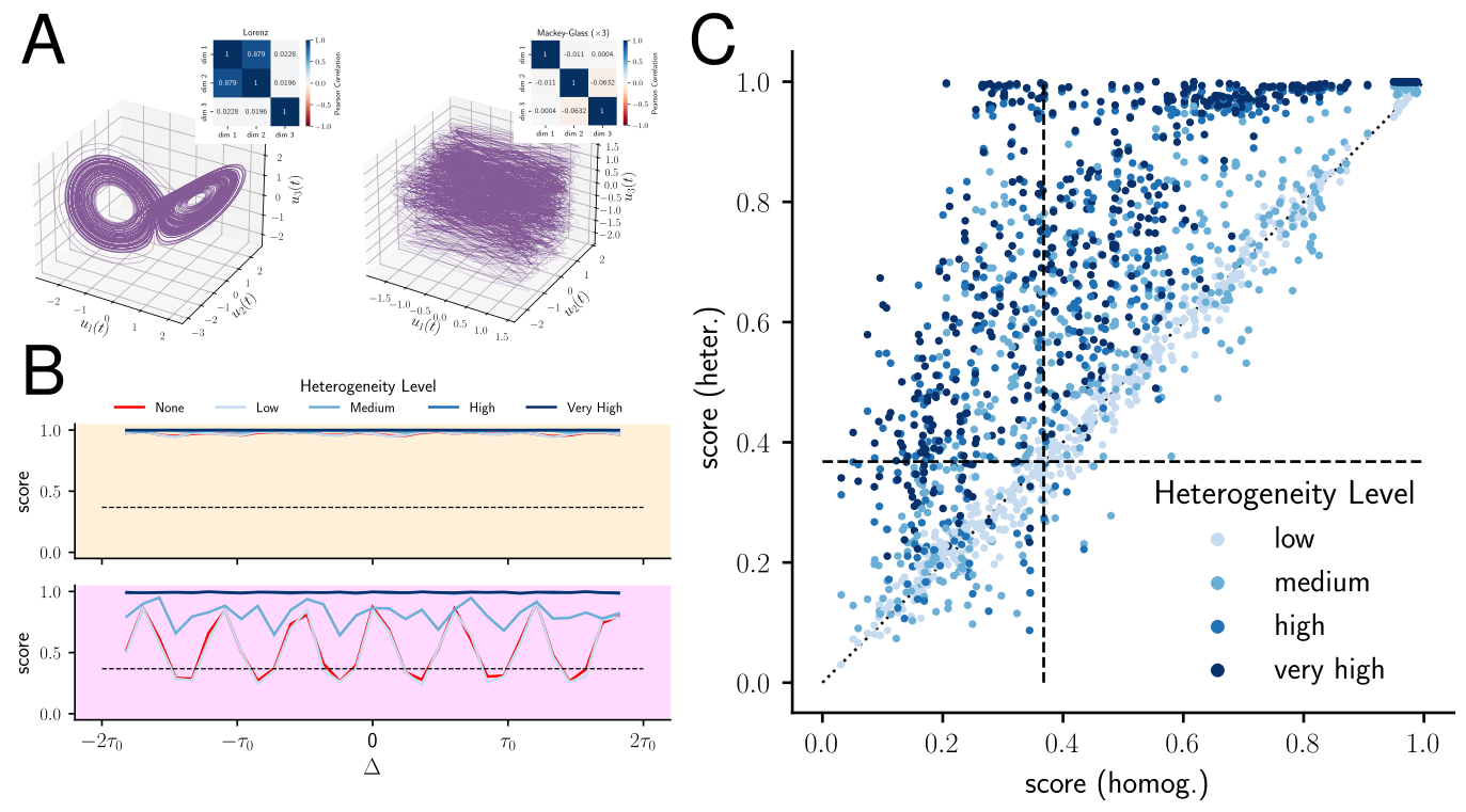
Figure A.1: Heterogeneity-induced performance gain is insensitive to the input type. (A) Components of a Lorenzian input (left) shows much higher structure than the concatenated MG process (right). Insets show cross-correlation between components. (B-D) Same as the ones in figure 2 but for concatenated MG processes. Note that the first input component is periodic. Thus, even a small amount of heterogeneity results in near perfect performance.

As figure A.1A shows, this construction effectively eliminated high cross-correlation between components and the low-dimensional manifold that exist in the case of Lorenzian input. Still, similar to the Lorenzian stimulus case, heterogeneous networks outperform homogeneous ones, both at the slice level (A.1B, A.1C), and holistically (A.1D). In particular, when the target function is predictable (as in figures A.1B-C, due to periodicity of the first component), even small degrees of heterogeneity tend to result in near perfect score.

Appendix B Applicability to spiking dynamics

Biological brains communicates with spikes. Is neuronal heterogeneity also effective under spiking dynamics? To answer this question, we carried out the same experiment with spiking neurons under identical configuration (c.f. section 6 for details). As figure B.1 shows, spiking dynamic shows a striking similarity to the rate-based one, with the more heterogeneous networks generally outperform their homogeneous analog.

Although in section 2.2 we argued that heterogeneity can be exploited in different dynamics, the specifics of each dynamic has crucial impact on the performance of certain tasks. An example, already visible in our result, is the tendency of spiking networks (heterogeneous or not) to perform better than chance, independent of the input type or hyperparameter values. We do not have an explanation for this surprising persistency. Although it is tempting to take interpret “better-than-chance” behavior as an evidence for superiority of spike communication than rate, this behavior may also very well be an artifact of our tasks choice. Therefore, further investigation is needed to clarify this tendency.

Figure B.1: Heterogeneity enhances computation with spikes. (A1) The score profiles of function approximation with spikes for linear (top) and quadratic (bottom) processing of time-shifted $k=1$st component of the Lorenzian input, similar to figure 2B. (B1) A holistic view of score improvement for all tasks and networks with all degree of heterogeneity, similar to figure 2C. (A2)-(B2) Same as above but for MG-based stimulus.

Appendix C Extended robustness results

C.1 Rate Dynamic

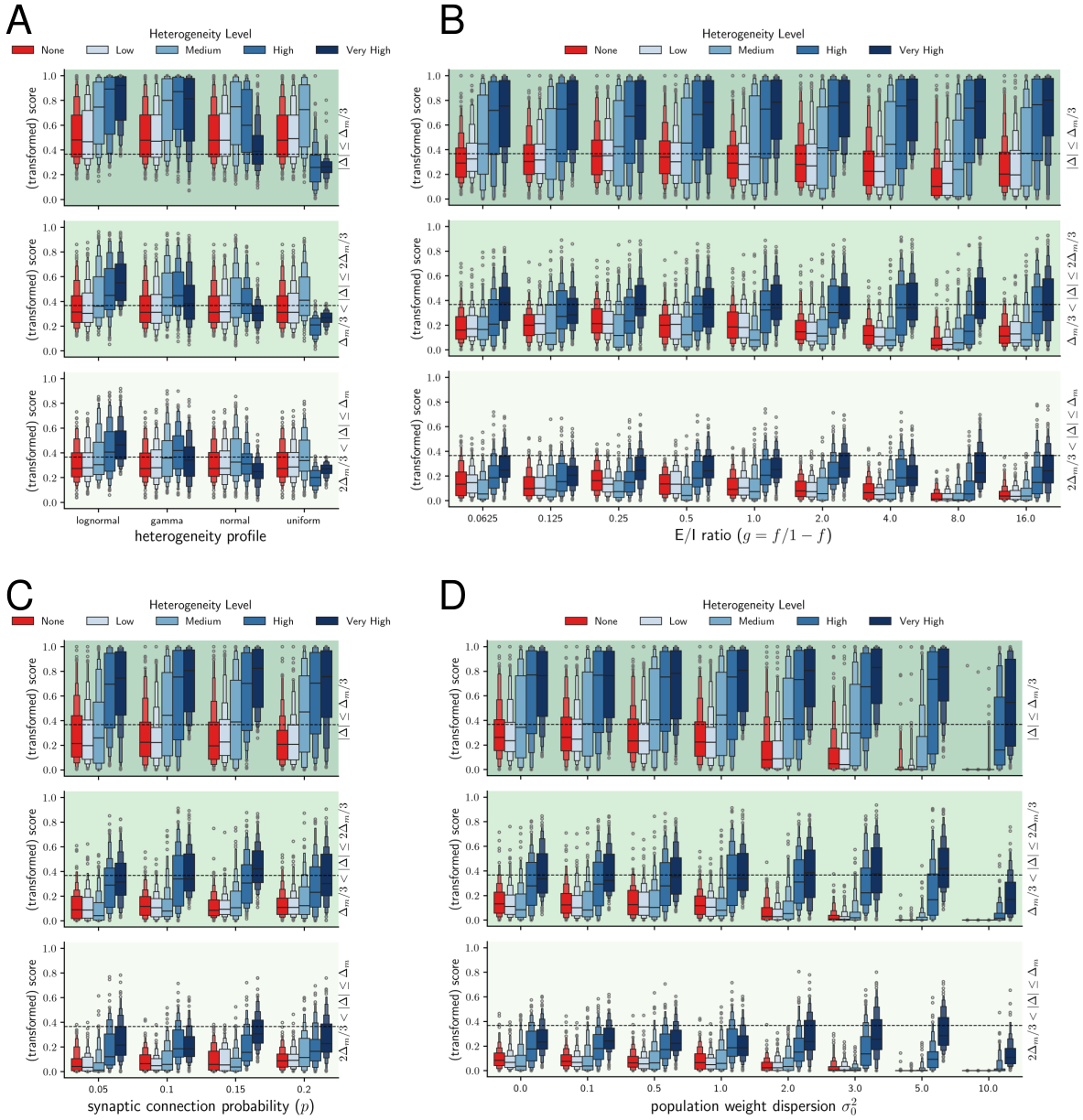
Figure C.1: Robustness of the rate-based networks. By default, we employ networks of size $N=250$, connection probabilty $p=0.1$, E/I ratio of $g=f/1-f=4$, weight dispersion $\sigma^{2}_{0}=1$, and recurrent gain $J=1$, whose neuronal time constant is sampled from a lognormal distribution with mean of $\operatorname{\mathbb{E}}[\tau]=\tau_{0}$ and different variance levels. Each panel shows the distribution networks score across 456 tasks as one of the following hyperparameter is varied: (A) heterogeneiety profile, (B) E/I ratio, (C) synaptic connection probability, and (D) weight dispersion. Note that only positively skewed heterogeneity profiles give raise to higher performance.

C.2 Spiking Dynamic

Figure C.2: Robustness of the spiking networks. same as figure C.1 but with spiking neurons. Hyperparameters that are varied are (A) recurrent gain, (B) network size, (C) average neuronal time constant, (cont.)

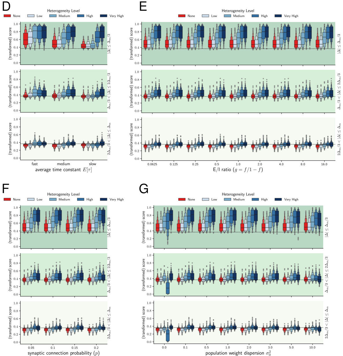
Figure C.2: (D) heterogeneity profile, (E) E/I ratio, (F) synaptic connection probability, and (G) weight dispersion.

Appendix D Transition to autonomous regime

The transition from input- to state-driven marks the point where the input-output mapping becomes nearly impossible. Under off-stimulus (or the small feedforward gain) condition, this transition occurs at the critical value $J_{c}=1$. Yet, for stimulated systems, this condition does not apply anymore, because even an inherently unstable system can be made stable via a proper input (e.g. inverted pendulum problem). In general, computing the transition boundary in driven and coupled systems is very challenging. However, as we outline below, with some very crude assumptions a lower bound for the transition boundary can be estimated.

Let us assume that, despite its time-dependent input, the system falls into one of its fixed points (FP), and only slightly fluctuates around it. In other words, we assume that the system has two main timescales which are largely separatable, a low-amplitude but fast timescales $\tau_{f}$ which is driven by the stimulus, and a large-amplitude by very slow one $\tau_{s}$ which originates from the dynamical structure. As such, one can use the linear stability analysis to estimate the critical synaptic gain $J_{c}$ (on the occupied FP). The Jacobian of equation 1 reads

$$\mathcal{J}_{ij}=\frac{\partial\dot{v}_{i}}{\partial v_{j}}=\frac{1}{\tau_{i}}(-\delta_{ij}+JW_{ij}r^{\prime}_{j})$$ (D1)

where $r^{\prime}$ is the derivative of the activation function and $\delta_{ij}$ is the Kronecker delta. The stability condition is $Re\{\lambda_{k}\}<0$ for all eigenvalue $\lambda_{k}$ of the Jacobian $\mathcal{J}$. The eigenvalues are predominantly determined by $W$, the recurrent connectivity matrix, which fortunately, due to its random structure, has well-known properties. According to the random matrix theory, [68, 80, 81, 82] the bulk of $W$’s eigenvalues lie on a disc with radius $R$ [82], whose value relates to the sparsity level $p$, fraction of excitatory neurons $f$, and the mean $mu_{x}$ and standard deviation $\sigma_{x}$ of synaptic strength of the population $x\in\{E,I\}$. Two analytical formulas for this radius has been proposed recently [83, 84]. However, only the latter is correct, which predicts the $R$ as

$$R^{2}=f[(1-p)\mu_{E}^{2}+\sigma_{E}^{2}]+(1-f)[(1-p)\mu_{I}^{2}+\sigma_{I}^{2}]$$ (D2)

from which eigenvalues of $\mathcal{J}$ can be deduced by considering the effect of each operation: The left multiplication by $1/\tau_{i}$ does not alter the spectrum, $\delta_{ij}$ just shifts it by 1 the to left, and $J$ scales all eigenvalues. The complication comes from the right (column-wise) multiplication by $r^{\prime}_{j}$ which has to be evaluated on the FP of equation 1. In principle, for different neurons, $r^{\prime}_{j}$ has different values. However, if we further assume that different components of $\bm{r}^{\prime}$ are i.i.d random variables, which are sampled independent of the process that has generated $W$, then the new matrix $Z=WD$, with $D=Diag(\bm{r}^{\prime})$., would also be a random matrix, with a spectrum conforming to the circle law. So, if assume that the underlying process that generates $\bm{r}^{\prime}$, or at least its statistics are known, then the spectrum of $\mathcal{J}$ will also be known. Note that statistics of $r^{\prime}_{j}$, when seen as a random variable, are different from that of $r^{\prime}_{j}(.)$ when seen as a function. Indeed, for a given choice of nonlinearity $r(.)$, the statistics of $r^{\prime}(.)$ is computable (either analytically or numerically). Yet, as a random variable, the realizations of $r^{\prime}_{j}$ (or its distribution) depend on the dynamic of the network. If we additionally assume ergodicity (at least on the occupied FP), then we can estimate the statistics of $r^{\prime}_{j}$ with that of its empirical temporal averages. Another approach, outlined in [83], is to use the central limit theorem, where distribution are known to conform to a normal one. However, since our networks sizes are much smaller than the thermodynamic limit, we decided to use the empirical estimates instead.

Following [84] and using the results from random matrix theory, the eigenvalues of $Z$ with $z_{ij}=w_{ij}r^{\prime}_{j}$ fall into the disc of radius $R_{Z}=\sqrt{N\operatorname{\mathbb{V}ar}[z_{ij}]}$. In what follows, we use subscripts $X(\in\{I,E\}$) and $D$ on expectations and variances to denote what underlying distribution is used to for marginalization. Direct computation yields

$$\operatorname{\mathbb{V}ar}[z_{ij}]=\operatorname{\mathbb{V}ar}_{X,D}[w_{ij}r^{\prime}_{j}]=f\operatorname{\mathbb{V}ar}_{E,D}[w_{ij}r^{\prime}_{j}]+(1-f)\operatorname{\mathbb{V}ar}_{I,D}[w_{ij}r^{\prime}_{j}]$$ (D3)

in which we used the fact that a fraction $f$ of all entries belong to the excitatory population and the rest are inhibitory. Now, the variance corresponding to population $x\in X=\{E,I\}$ reads:

$$\operatorname{\mathbb{V}ar}_{x}[w_{ij}r^{\prime}_{j}] =\operatorname{\mathbb{E}}_{x}[w_{ij}^{2}r_{j}^{{}^{\prime}2}]-\operatorname{\mathbb{E}}_{x}[w_{ij}r^{\prime}_{j}]^{2}$$ (D4)

$$=\operatorname{\mathbb{E}}_{x}[w_{ij}^{2}]\operatorname{\mathbb{E}}_{D}[r_{j}^{{}^{\prime}2}]-\operatorname{\mathbb{E}}_{x}[w_{ij}]^{2}\operatorname{\mathbb{E}}_{D}[r^{\prime}_{j}]^{2}$$ (independence) (D5)

$$=p(\mu_{x}^{2}+\sigma_{x}^{2})\operatorname{\mathbb{E}}_{D}[r_{j}^{{}^{\prime}2}]-(p\mu_{x})^{2}\operatorname{\mathbb{E}}_{D}[r^{\prime}_{j}]^{2}$$ (sparsity) (D6)

If we denote the first and second moments of $r^{\prime}$ by $d_{1}$ and $d_{2}^{2}$ respectively, the total variance of elements of $Z$ would be:

$$\operatorname{\mathbb{V}ar}[z_{ij}] =pf\Big{[}d_{2}^{2}(\mu_{E}^{2}+\sigma_{E}^{2})-p\mu_{E}^{2}d_{1}^{2}\Big{]}+p(1-f)\Big{[}d_{2}^{2}(\mu_{I}^{2}+\sigma_{I}^{2})-p\mu_{E}^{2}d_{1}^{2}\Big{]}$$ (D7)

$$=p\Big{[}d_{2}^{2}\big{[}f(\mu_{E}^{2}+\sigma_{E}^{2})+(1-f)(\mu_{I}^{2}+\sigma_{I}^{2})\big{]}-d_{1}^{2}p\big{[}f\mu_{E}^{2}+(1-f)\mu_{E}^{2})\big{]}\Big{]}$$ (D8)

which is true even it the network is unbalanced. For our networks, we usually used $p=0.1,f=0.8,\mu_{e}=1/\sqrt{Np},\sigma_{e}=\sigma_{i}=\sigma_{0}/\sqrt{Np}=1/\sqrt{Np}$. Moreover, from the balance condition we have $\mu_{i}=-\frac{f}{(1-f)\sqrt{Np}}=-4/\sqrt{Np}$. Substituting these numbers results in D8 yields this simple relationship between the radius $R_{Z}$ and the first two statistics of $r^{\prime}$:

$$R_{Z}^{2}=5d_{2}^{2}-0.4d_{1}^{2}$$ (D9)

Once the first two moments of $r^{\prime}$ are empirically found, the critical value of gain, follows from the following simple inequality:

$$-1+JR_{Z}<0\longrightarrow J_{c}=\frac{1}{R_{Z}}$$ (D10)

However, the above condition must be verified self-consistently: if the $J\leq J_{c}$, then the system, in expectation, is linearly stable, and can give rise to a stationary distribution of $r^{\prime}$. Otherwise, the system is linearly unstable, which violates the stationarity of $r^{\prime}_{j}$ process. Thus, the linear stability analysis is only valid if $J_{c}\leq J$.

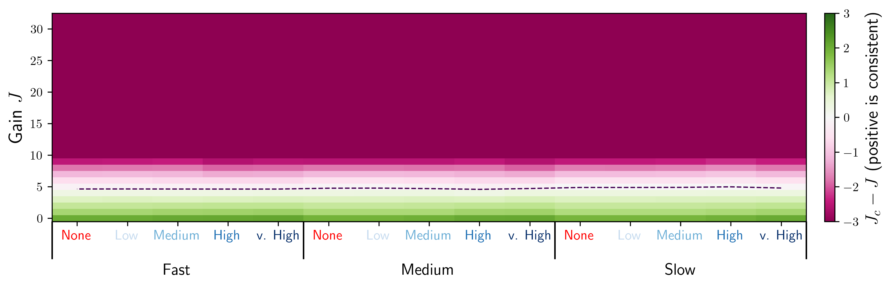
Figure D.1: Self-consistency indicator indicates the location of critical gran $J_{c}$. The difference between estimated critical gain $J_{c}$ and the actual network $J$ are plotted versus $J$ for all networks. The main assumption behind equation D10 is valid only when $J\leq J_{c}$. The dashed line at $J=J_{c}\approx 5$ delineates the border of self-consistency. For $J>5$, linear stability predicts an unstable system, which contradicts the assumption of $r^{\prime}_{j}$ being a stationarty random process.

Figure D.1 shows the self-consistency criterion, $J_{c}-J$, versus $J$, for different networks with various combinations of neuronal mean and variances. As $J$ increases and networks become more state-driven, self-consistency gradually degrades and crosses the zero as network gain reaches the value of $J\approx 5$ (the dashed line). Interestingly, the heterogeneity does not affect the (linear) stability directly (as all networks loose consistency, more or less, at the same gain). This is largely due to the fact we modelled the recurrent connections independent of time scales, which resulted to a row-wise multiplication in equation D2 that leaves the spectrum intact. Some authors, however, fuse the $1/\tau_{i}$ term in equation 1 in to $W$. In this case, none of the analysis above hold.

Appendix E Task Complexity is Dominated by the Temporal Shift

To classify tasks into different complexity tiers, we color-coded the score comparison plots by various parameters. Figure E.1 shows one such example. Our experiments suggested that input time-shift has the highest impact in on the performance. Thus, we grouped tasks into three different tiers based on their value of $|\Delta|$.

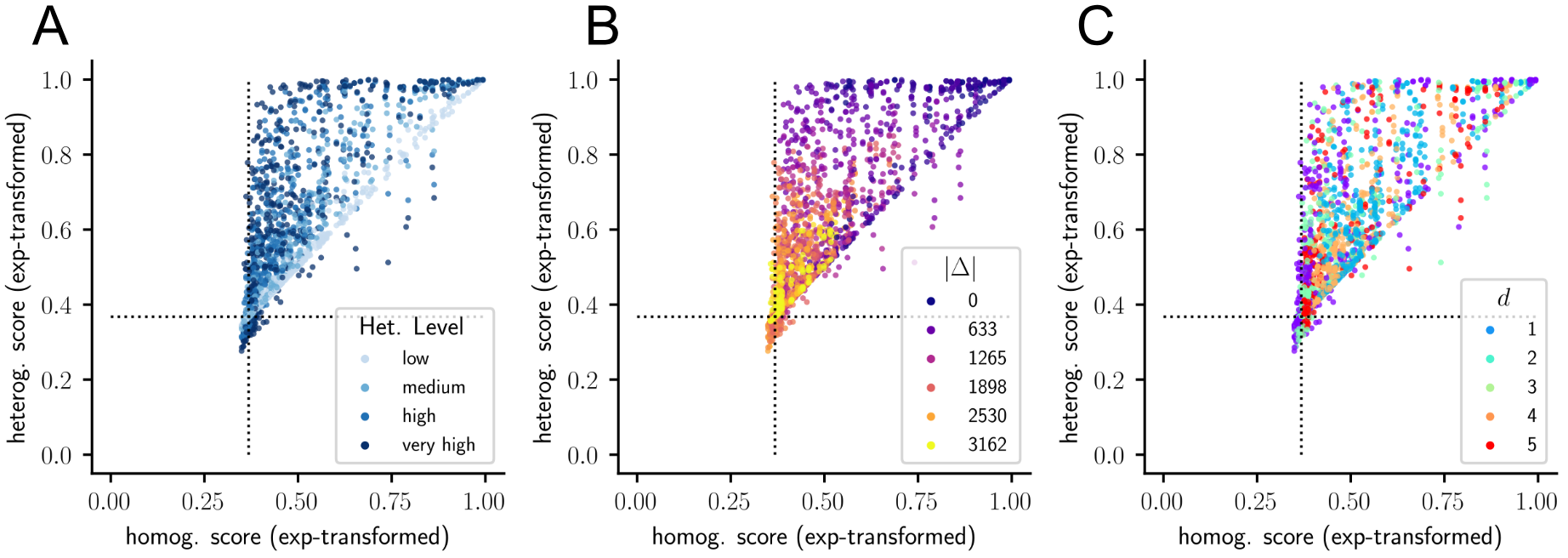
Figure E.1: Complexity of the task is mostly driven by time-shift $|\Delta|$. Score comparison plot color-coded by (A) heterogeneity level, (B) time-shift $|\Delta|$, and (C) the nonlinearity $d$.

References

- [1] Chia-Chien Chen, Svetlana Abrams, Alex Pinhas and Joshua C. Brumberg “Morphological Heterogeneity of Layer VI Neurons in Mouse Barrel Cortex” In Journal of Comparative Neurology 512.6, 2009, pp. 726–746 DOI: 10.1002/cne.21926
- [2] Hongkui Zeng and Joshua R. Sanes “Neuronal Cell-Type Classification: Challenges, Opportunities and the Path Forward” In Nature Reviews Neuroscience 18.9 Nature Publishing Group, 2017, pp. 530–546 DOI: 10.1038/nrn.2017.85
- [3] Stephanie C Seeman et al. “Sparse Recurrent Excitatory Connectivity in the Microcircuit of the Adult Mouse and Human Cortex” In eLife 7 eLife Sciences Publications, Ltd, 2018, pp. e37349 DOI: 10.7554/eLife.37349
- [4] J. Hasse, Elise M. Bragg, Allison J. Murphy and Farran Briggs “Morphological Heterogeneity among Corticogeniculate Neurons in Ferrets: Quantification and Comparison with a Previous Report in Macaque Monkeys” In Journal of Comparative Neurology 527.3, 2019, pp. 546–557 DOI: 10.1002/cne.24451
- [5] Renchao Chen et al. “Decoding Molecular and Cellular Heterogeneity of Mouse Nucleus Accumbens” In Nature Neuroscience 24.12 Nature Publishing Group, 2021, pp. 1757–1771 DOI: 10.1038/s41593-021-00938-x
- [6] Zizhen Yao et al. “A Taxonomy of Transcriptomic Cell Types across the Isocortex and Hippocampal Formation” In Cell 184.12, 2021, pp. 3222–3241.e26 DOI: 10.1016/j.cell.2021.04.021
- [7] Luke Campagnola et al. “Local Connectivity and Synaptic Dynamics in Mouse and Human Neocortex” In Science 375.6585 American Association for the Advancement of Science, 2022, pp. eabj5861 DOI: 10.1126/science.abj5861
- [8] Zizhen Yao et al. “A High-Resolution Transcriptomic and Spatial Atlas of Cell Types in the Whole Mouse Brain” In Nature 624.7991 Nature Publishing Group, 2023, pp. 317–332 DOI: 10.1038/s41586-023-06812-z
- [9] Jonah Langlieb et al. “The Molecular Cytoarchitecture of the Adult Mouse Brain” In Nature 624.7991 Nature Publishing Group, 2023, pp. 333–342 DOI: 10.1038/s41586-023-06818-7
- [10] David Golomb and John Rinzel “Dynamics of Globally Coupled Inhibitory Neurons with Heterogeneity” In Physical Review E 48.6 American Physical Society, 1993, pp. 4810–4814 DOI: 10.1103/PhysRevE.48.4810
- [11] Stefano Luccioli and Antonio Politi “Irregular Collective Behavior of Heterogeneous Neural Networks” In Physical Review Letters 105.15 American Physical Society, 2010, pp. 158104 DOI: 10.1103/PhysRevLett.105.158104
- [12] David Angulo-Garcia, Stefano Luccioli, Simona Olmi and Alessandro Torcini “Death and Rebirth of Neural Activity in Sparse Inhibitory Networks” In New Journal of Physics 19.5 IOP Publishing, 2017, pp. 053011 DOI: 10.1088/1367-2630/aa69ff
- [13] Stefano Luccioli, David Angulo-Garcia and Alessandro Torcini “Neural Activity of Heterogeneous Inhibitory Spiking Networks with Delay” In Physical Review E 99.5, 2019, pp. 052412 DOI: 10.1103/PhysRevE.99.052412
- [14] Richard Gast, Sara A. Solla and Ann Kennedy “Neural Heterogeneity Controls Computations in Spiking Neural Networks” In Proceedings of the National Academy of Sciences 121.3 Proceedings of the National Academy of Sciences, 2024, pp. e2311885121 DOI: 10.1073/pnas.2311885121
- [15] Srdjan Ostojic, Nicolas Brunel and Vincent Hakim “Synchronization Properties of Networks of Electrically Coupled Neurons in the Presence of Noise and Heterogeneities” In Journal of Computational Neuroscience 26.3, 2009, pp. 369–392 DOI: 10.1007/s10827-008-0117-3
- [16] Toni Pérez, Claudio R. Mirasso, Raúl Toral and James D. Gunton “The Constructive Role of Diversity in the Global Response of Coupled Neuron Systems” In Philosophical Transactions of the Royal Society A: Mathematical, Physical and Engineering Sciences 368.1933 Royal Society, 2010, pp. 5619–5632 DOI: 10.1098/rsta.2010.0264
- [17] Jorge F. Mejias and André Longtin “Differential Effects of Excitatory and Inhibitory Heterogeneity on the Gain and Asynchronous State of Sparse Cortical Networks” In Frontiers in Computational Neuroscience 8 Frontiers, 2014 DOI: 10.3389/fncom.2014.00107
- [18] Maoz Shamir and Haim Sompolinsky “Implications of Neuronal Diversity on Population Coding” In Neural Computation 18.8, 2006, pp. 1951–1986 DOI: 10.1162/neco.2006.18.8.1951
- [19] Shreejoy J. Tripathy, Krishnan Padmanabhan, Richard C. Gerkin and Nathaniel N. Urban “Intermediate Intrinsic Diversity Enhances Neural Population Coding” In Proceedings of the National Academy of Sciences 110.20 Proceedings of the National Academy of Sciences, 2013, pp. 8248–8253 DOI: 10.1073/pnas.1221214110
- [20] Manuel Beiran, Alexandra Kruscha, Jan Benda and Benjamin Lindner “Coding of Time-Dependent Stimuli in Homogeneous and Heterogeneous Neural Populations” In Journal of Computational Neuroscience 44.2, 2018, pp. 189–202 DOI: 10.1007/s10827-017-0674-4
- [21] Matteo Di Volo and Alain Destexhe “Optimal Responsiveness and Information Flow in Networks of Heterogeneous Neurons” In Scientific Reports 11.1 Nature Publishing Group, 2021, pp. 17611 DOI: 10.1038/s41598-021-96745-2
- [22] Alain Destexhe “Noise Enhancement of Neural Information Processing” In Entropy 24.12 Multidisciplinary Digital Publishing Institute, 2022, pp. 1837 DOI: 10.3390/e24121837
- [23] Krishnan Padmanabhan and Nathaniel N. Urban “Intrinsic Biophysical Diversity Decorrelates Neuronal Firing While Increasing Information Content” In Nature Neuroscience 13.10 Nature Publishing Group, 2010, pp. 1276–1282 DOI: 10.1038/nn.2630
- [24] Kamilla Angelo et al. “A Biophysical Signature of Network Affiliation and Sensory Processing in Mitral Cells” In Nature 488.7411 Nature Publishing Group, 2012, pp. 375–378 DOI: 10.1038/nature11291
- [25] Ann Kennedy et al. “A Temporal Basis for Predicting the Sensory Consequences of Motor Commands in an Electric Fish” In Nature Neuroscience 17.3 Nature Publishing Group, 2014, pp. 416–422 DOI: 10.1038/nn.3650
- [26] Chris I. De Zeeuw et al. “Heterogeneous Encoding of Temporal Stimuli in the Cerebellar Cortex” In Nature Communications 14.1 Nature Publishing Group, 2023, pp. 7581 DOI: 10.1038/s41467-023-43139-9
- [27] Lars A. Holmstrom, Lonneke B.. Eeuwes, Patrick D. Roberts and Christine V. Portfors “Efficient Encoding of Vocalizations in the Auditory Midbrain” In The Journal of Neuroscience 30.3, 2010, pp. 802–819 DOI: 10.1523/JNEUROSCI.1964-09.2010
- [28] Takashi Matsubara “Conduction Delay Learning Model for Unsupervised and Supervised Classification of Spatio-Temporal Spike Patterns” In Frontiers in Computational Neuroscience 11 Frontiers, 2017 DOI: 10.3389/fncom.2017.00104
- [29] Wei Fang et al. “Incorporating Learnable Membrane Time Constant to Enhance Learning of Spiking Neural Networks”, 2021 arXiv: http://arxiv.org/abs/2007.05785
- [30] Nicolas Perez-Nieves, Vincent C.. Leung, Pier Luigi Dragotti and Dan F.. Goodman “Neural Heterogeneity Promotes Robust Learning” In Nature Communications 12.1, 2021, pp. 5791 DOI: 10.1038/s41467-021-26022-3
- [31] Chloe N. Winston, Dana Mastrovito, Eric Shea-Brown and Stefan Mihalas “Heterogeneity in Neuronal Dynamics Is Learned by Gradient Descent for Temporal Processing Tasks” In Neural Computation 35.4, 2023, pp. 555–592 DOI: 10.1162/neco_a_01571
- [32] Karim G. Habashy, Benjamin D. Evans, Dan F.. Goodman and Jeffrey S. Bowers “Adapting to Time: Why Nature Evolved a Diverse Set of Neurons”, 2024 DOI: 10.48550/arXiv.2404.14325
- [33] Hanle Zheng et al. “Temporal Dendritic Heterogeneity Incorporated with Spiking Neural Networks for Learning Multi-Timescale Dynamics” In Nature Communications 15.1 Nature Publishing Group, 2024, pp. 277 DOI: 10.1038/s41467-023-44614-z
- [34] David Zipser and Richard A. Andersen “A Back-Propagation Programmed Network That Simulates Response Properties of a Subset of Posterior Parietal Neurons” In Nature 331.6158 Nature Publishing Group, 1988, pp. 679–684 DOI: 10.1038/331679a0
- [35] Yuhang Song, Thomas Lukasiewicz, Zhenghua Xu and Rafal Bogacz “Can the Brain Do Backpropagation? — Exact Implementation of Backpropagation in Predictive Coding Networks” In Advances in Neural Information Processing Systems 33 Curran Associates, Inc., 2020, pp. 22566–22579 URL: https://proceedings.neurips.cc/paper/2020/hash/fec87a37cdeec1c6ecf8181c0aa2d3bf-Abstract.html
- [36] Beren Millidge, Alexander Tschantz and Christopher L. Buckley “Predictive Coding Approximates Backprop along Arbitrary Computation Graphs”, 2020 DOI: 10.48550/arXiv.2006.04182
- [37] Alexander Meulemans et al. “Credit Assignment in Neural Networks through Deep Feedback Control”, 2022 DOI: 10.48550/arXiv.2106.07887
- [38] Pau Vilimelis Aceituno, Sander Haan, Reinhard Loidl and Benjamin F. Grewe “Hierarchical Target Learning in the Mammalian Neocortex: A Pyramidal Neuron Perspective”, 2024, pp. 2024.04.10.588837 DOI: 10.1101/2024.04.10.588837
- [39] C. Vreeswijk and H. Sompolinsky “Chaos in Neuronal Networks with Balanced Excitatory and Inhibitory Activity” In Science American Association for the Advancement of Science, 1996 URL: https://www.science.org/doi/abs/10.1126/science.274.5293.1724
- [40] Nicolas Brunel “Dynamics of Sparsely Connected Networks of Excitatory and Inhibitory Spiking Neurons” In Journal of Computational Neuroscience 8.3, 2000, pp. 183–208 DOI: 10.1023/A:1008925309027
- [41] Joni Dambre, David Verstraeten, Benjamin Schrauwen and Serge Massar “Information Processing Capacity of Dynamical Systems” In Scientific Reports 2.1 Nature Publishing Group, 2012, pp. 514 DOI: 10.1038/srep00514
- [42] Tomoyuki Kubota, Hirokazu Takahashi and Kohei Nakajima “Unifying Framework for Information Processing in Stochastically Driven Dynamical Systems” In Physical Review Research 3.4, 2021, pp. 043135 DOI: 10.1103/PhysRevResearch.3.043135
- [43] S. Boyd and L. Chua “Fading Memory and the Problem of Approximating Nonlinear Operators with Volterra Series” In IEEE Transactions on Circuits and Systems 32.11, 1985, pp. 1150–1161 DOI: 10.1109/TCS.1985.1085649
- [44] Wolfgang Maass, Thomas Natschläger and Henry Markram “Real-Time Computing Without Stable States: A New Framework for Neural Computation Based on Perturbations” In Neural Computation 14.11, 2002, pp. 2531–2560 DOI: 10.1162/089976602760407955
- [45] Herbert Jaeger “The“ Echo State” Approach to Analysing and Training Recurrent Neural Networks-with an Erratum Note”’ In Bonn, Germany: German National Research Center for Information Technology GMD Technical Report 148, 2001
- [46] F. Bullo “Contraction Theory for Dynamical Systems” Kindle Direct Publishing, 2024 URL: https://fbullo.github.io/ctds
- [47] Steven H. Strogatz “Nonlinear Dynamics and Chaos: With Applications to Physics, Biology, Chemistry, and Engineering” Boulder, CO: Westview Press, a member of the Perseus Books Group, 2015
- [48] Daniel J. Amit “Modeling Brain Function: The World of Attractor Neural Networks” Cambridge University Press, 1989 GOOGLEBOOKS: fvLYch1yQncC
- [49] Mikail Khona and Ila R. Fiete “Attractor and Integrator Networks in the Brain” In Nature Reviews Neuroscience Nature Publishing Group, 2022, pp. 1–23 DOI: 10.1038/s41583-022-00642-0
- [50] H. Sompolinsky, A. Crisanti and H.. Sommers “Chaos in Random Neural Networks” In Physical Review Letters 61.3 American Physical Society, 1988, pp. 259–262 DOI: 10.1103/PhysRevLett.61.259
- [51] D. Hansel and H. Sompolinsky “Synchronization and Computation in a Chaotic Neural Network” In Physical Review Letters 68.5, 1992, pp. 718–721 DOI: 10.1103/PhysRevLett.68.718
- [52] B. Doyon, B. Cessac, M. Quoy and M. Samuelides “On Bifurcations and Chaos in Random Neural Networks” In Acta Biotheoretica 42.2, 1994, pp. 215–225 DOI: 10.1007/BF00709492
- [53] D.. Hubel and T.. Wiesel “Receptive Fields, Binocular Interaction and Functional Architecture in the Cat’s Visual Cortex” In The Journal of Physiology 160.1, 1962, pp. 106–154 DOI: 10.1113/jphysiol.1962.sp006837
- [54] D.. Hubel and T.. Wiesel “Receptive Fields and Functional Architecture of Monkey Striate Cortex” In The Journal of Physiology 195.1, 1968, pp. 215–243 DOI: 10.1113/jphysiol.1968.sp008455
- [55] Alberto Bernacchia, Hyojung Seo, Daeyeol Lee and Xiao-Jing Wang “A Reservoir of Time Constants for Memory Traces in Cortical Neurons” In Nature neuroscience 14.3, 2011, pp. 366–372 DOI: 10.1038/nn.2752
- [56] Stefan J. Kiebel, Jean Daunizeau and Karl J. Friston “A Hierarchy of Time-Scales and the Brain” In PLOS Computational Biology 4.11 Public Library of Science, 2008, pp. e1000209 DOI: 10.1371/journal.pcbi.1000209
- [57] Sean E. Cavanagh, Laurence T. Hunt and Steven W. Kennerley “A Diversity of Intrinsic Timescales Underlie Neural Computations” In Frontiers in Neural Circuits 14 Frontiers, 2020 DOI: 10.3389/fncir.2020.615626
- [58] J J Hopfield “Neural Networks and Physical Systems with Emergent Collective Computational Abilities.” In Proceedings of the National Academy of Sciences 79.8, 1982, pp. 2554–2558 DOI: 10.1073/pnas.79.8.2554
- [59] Amadeus Maes, Mauricio Barahona and Claudia Clopath “Learning Spatiotemporal Signals Using a Recurrent Spiking Network That Discretizes Time” In PLOS Computational Biology 16.1 Public Library of Science, 2020, pp. e1007606 DOI: 10.1371/journal.pcbi.1007606
- [60] Amadeus Maes, Mauricio Barahona and Claudia Clopath “Learning Compositional Sequences with Multiple Time Scales through a Hierarchical Network of Spiking Neurons” In PLOS Computational Biology 17.3 Public Library of Science, 2021, pp. e1008866 DOI: 10.1371/journal.pcbi.1008866
- [61] Henrik Lindén, Peter C. Petersen, Mikkel Vestergaard and Rune W. Berg “Movement Is Governed by Rotational Neural Dynamics in Spinal Motor Networks” In Nature 610.7932 Nature Publishing Group, 2022, pp. 526–531 DOI: 10.1038/s41586-022-05293-w
- [62] Christopher D. Harvey, Philip Coen and David W. Tank “Choice-Specific Sequences in Parietal Cortex during a Virtual-Navigation Decision Task” In Nature 484.7392 Nature Publishing Group, 2012, pp. 62–68 DOI: 10.1038/nature10918
- [63] Eva Pastalkova, Vladimir Itskov, Asohan Amarasingham and György Buzsáki “Internally Generated Cell Assembly Sequences in the Rat Hippocampus” In Science 321.5894 American Association for the Advancement of Science, 2008, pp. 1322–1327 DOI: 10.1126/science.1159775
- [64] James M Murray and G Sean Escola “Learning Multiple Variable-Speed Sequences in Striatum via Cortical Tutoring” In eLife 6 eLife Sciences Publications, Ltd, 2017, pp. e26084 DOI: 10.7554/eLife.26084
- [65] Andrew B. Lehr, Arvind Kumar and Christian Tetzlaff “Sparse Clustered Inhibition Projects Sequential Activity onto Unique Neural Subspaces”, 2023, pp. 2023.09.15.557865 DOI: 10.1101/2023.09.15.557865
- [66] Wr Softky and C Koch “The Highly Irregular Firing of Cortical Cells Is Inconsistent with Temporal Integration of Random EPSPs” In The Journal of Neuroscience 13.1, 1993, pp. 334–350 DOI: 10.1523/JNEUROSCI.13-01-00334.1993
- [67] G.. Holt, W.. Softky, C. Koch and R.. Douglas “Comparison of Discharge Variability in Vitro and in Vivo in Cat Visual Cortex Neurons” In Journal of Neurophysiology 75.5, 1996, pp. 1806–1814 DOI: 10.1152/jn.1996.75.5.1806
- [68] Kanaka Rajan and L.. Abbott “Eigenvalue Spectra of Random Matrices for Neural Networks” In Physical Review Letters 97.18 American Physical Society, 2006, pp. 188104 DOI: 10.1103/PhysRevLett.97.188104
- [69] Nathan Trouvain, Luca Pedrelli, Thanh Trung Dinh and Xavier Hinaut “ReservoirPy: An Efficient and User-Friendly Library to Design Echo State Networks” In Artificial Neural Networks and Machine Learning – ICANN 2020 Cham: Springer International Publishing, 2020, pp. 494–505 DOI: 10.1007/978-3-030-61616-8_40
- [70] Edward N. Lorenz “Deterministic Nonperiodic Flow” In Journal of the Atmospheric Sciences 20.2 American Meteorological Society, 1963, pp. 130–141 DOI: 10.1175/1520-0469(1963)020<0130:DNF>2.0.CO;2
- [71] Michael C. Mackey and Leon Glass “Oscillation and Chaos in Physiological Control Systems” In Science 197.4300 American Association for the Advancement of Science, 1977, pp. 287–289 DOI: 10.1126/science.267326
- [72] Hendrik Wernecke, Bulcsú Sándor and Claudius Gros “Chaos in Time Delay Systems, an Educational Review” In Physics Reports 824, 2019, pp. 1–40 DOI: 10.1016/j.physrep.2019.08.001
- [73] John D. Hunter “Matplotlib: A 2D Graphics Environment” In Computing in Science & Engineering 9.3, 2007, pp. 90–95 DOI: 10.1109/MCSE.2007.55
- [74] Michael L. Waskom “Seaborn: Statistical Data Visualization” In Journal of Open Source Software 6.60, 2021, pp. 3021 DOI: 10.21105/joss.03021
- [75] John Garrett et al. “Garrettj403/SciencePlots: 2.1.1”, 2023 Zenodo DOI: 10.5281/zenodo.10206719
- [76] Charles R. Harris et al. “Array Programming with NumPy” In Nature 585.7825 Nature Publishing Group, 2020, pp. 357–362 DOI: 10.1038/s41586-020-2649-2
- [77] Pauli Virtanen et al. “SciPy 1.0: Fundamental Algorithms for Scientific Computing in Python” In Nature Methods 17.3 Nature Publishing Group, 2020, pp. 261–272 DOI: 10.1038/s41592-019-0686-2
- [78] Joblib Development Team “Joblib: running Python functions as pipeline jobs”, 2020 URL: https://joblib.readthedocs.io/
- [79] Marcel Stimberg, Romain Brette and Dan FM Goodman “Brian 2, an Intuitive and Efficient Neural Simulator” In eLife 8, 2019, pp. e47314 DOI: 10.7554/eLife.47314
- [80] Terence Tao and Van Vu “Random Matrices: The Circular Law”, 2008 DOI: 10.48550/arXiv.0708.2895
- [81] Terence Tao “Outliers in the Spectrum of Iid Matrices with Bounded Rank Perturbations” arXiv, 2014 DOI: 10.48550/arXiv.1012.4818
- [82] Georgia Christodoulou and Tim Vogels “The Eigenvalue Value (in Neuroscience)”, 2022 DOI: 10.31219/osf.io/evqhy
- [83] Axel Hutt, Scott Rich, Taufik A. Valiante and Jérémie Lefebvre “Intrinsic Neural Diversity Quenches the Dynamic Volatility of Neural Networks” In Proceedings of the National Academy of Sciences 120.28 Proceedings of the National Academy of Sciences, 2023, pp. e2218841120 DOI: 10.1073/pnas.2218841120
- [84] Isabelle D. Harris, Hamish Meffin, Anthony N. Burkitt and Andre D.. Peterson “Effect of Sparsity on Network Stability in Random Neural Networks Obeying Dale’s Law” In Physical Review Research 5.4, 2023, pp. 043132 DOI: 10.1103/PhysRevResearch.5.043132