Enhancing low-temperature quantum thermometry via sequential measurements

Abstract

We propose a sequential measurement protocol for accurate low-temperature estimation. The resulting correlated outputs significantly enhance the low temperature precision compared to that of the independent measurement scheme. This enhancement manifests a Heisenberg scaling of the signal-to-noise ratio for small measurement numbers $N$. Detailed analysis reveals that the final precision is determined by the pair correlation of the sequential outputs, which produces a dependence $N^{2}$ on the signal-to-noise ratio. Remarkably, we find that quantum thermometry within the sequential protocol functions as a high-resolution quantum spectroscopy of the thermal noise, underscoring the pivotal role of the sequential measurements in enhancing the spectral resolution and the temperature estimation precision. Our methodology incorporates sequential measurement into low-temperature quantum thermometry, representing an important advancement in low-temperature measurement.

I Introduction

Accurate temperature measurement of ultracold systems is crucial for quantifying and controlling ultracold atoms, which are central to the study of quantum many-body physics and the development of advanced quantum techniques [1, 2, 3, 4]. The standard measurement method is based on the time-of-flight technique, which, however, is destructive [5, 6]. Many nondestructive measurement techniques have been proposed [7, 8, 9, 10, 11]. An extreme example is to map the temperature estimation to a phase estimation problem, where the temperature is measured using a Ramsey interferometry [12, 13, 14, 15]. Without heat exchange between the thermometer and the sample, the phase estimation scheme provides an almost nondestructive way to detect temperature [9, 11].

In the low-temperature regime, the quantum thermometer encounters the error divergence problem [16, 17, 18], which arises due to the vanishing heat capacity of the thermometer in the ultracold scenario. Various quantum features have been proposed to improve the precision of measurement, such as strong coupling [7, 8, 19, 20], quantum correlations [21, 22], quantum criticality [23, 24, 25, 26], and quantum non-Markovianity [27, 28]. Among them, the correlation between the thermometer and the sample is a crucial resource for low-temperature quantum thermometry [29]. The sample-induced correlation between different thermometers in the parallel strategy has been shown to be helpful in improving the precision of low temperature [30, 31, 32]. Beyond the parallel strategy, sample-induced correlations are also present within a sequential protocol between sequential outputs [33, 34, 21, 35, 36]. The quantum thermometry based on the sequential protocol has been proposed in Refs. [34, 21], however, a negative conclusion is obtained that there is no precision enhancement compared to the independent protocol [34].

In stark contrast to parallel strategies that take advantage of spatial correlation or entanglement [37, 38], the sequential protocol utilizes temporal correlation or coherence to improve measurement precision [33, 39]. Sequential protocols have been used to measure quantum nonlinear spectroscopy [40, 41, 42, 43, 44, 45], which exceeds the resolution limitations set by the lifetime of the probe, allowing for a high spectral resolution [46, 47, 48, 49, 50, 51]. Nevertheless, the potential benefits conferred by temporal correlation within the domain of quantum thermometry have yet to be observed.

In this paper, we study the low-temperature quantum thermometry in a sequential protocol. Our goal is to investigate the role of temporal correlation in low-temperature quantum thermometry. We find that precision can be significantly enhanced by sequential measurements in the regime $\hbar\beta/t_{2}\gg 1$, where $\beta=1/K_{B}T$ denotes the thermodynamic beta and $t_{2}$ denotes the coherence time of the thermometer. A typical example is a pK sample measured with a microsecond coherence time thermometer, which yields $\hbar\beta/t_{2}\approx 7\times 10^{3}$. Specifically, a Heisenberg scaling is achieved when the number of sequential measurements satisfies $N\ll\hbar\beta/t_{2}$. On the other hand, when $N\gg\hbar\beta/t_{2}$, this scaling changes to the standard quantum limit, but with a significant improvement in precision compared to the independent measurement scheme. Detail analysis shows that pair correlations in these measurement outputs play a central role in precision enhancement. Given that the pair correlation is intrinsically linked to the noise spectrum of the thermal sample, we elucidate that the temperature estimation process via sequential measurement is fundamentally intertwined with the high-resolution spectroscopy of the noise.

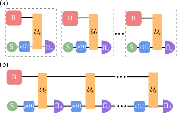
Figure 1: Independent measurement scheme (a) and sequential measurement scheme (b) for temperature estimation. The thermal sample and the thermometer are denoted as “B” and “S”, respectively. Each block in (a) indicates a temperature estimation process. Here, $\rho(0)$ denotes the initial state preparation, $\mathcal{U}_{t}$ denotes the evolution of the thermometer-sample system, and $\hat{\Pi}_{x}$ and $\hat{\Pi}_{\theta}$ indicate the measurement along $x$ and $\vec{e}_{\theta}:=\cos\theta\vec{e}_{x}+\sin\theta\vec{y}$ direction, respectively.

II low-temperature quantum thermometry

We consider a temperature estimation process based on Ramsey interferometry. The thermometer is modeled as a two-level system, and the thermal sample is represented as a multimode bosonic reservoir with a specific temperature $T$. The Hamiltonian of the thermometer in the thermal sample reads $\hat{H}(\tau)=\hat{X}(\tau)\hat{\sigma}_{z}$ [9, 11], where $\hat{\sigma}_{z}$ is the Pauli matrix and $\hat{X}(\tau)$ denotes the noise operator of the sample with the following expression

$$\hat{X}(\tau)=\sum_{k}\hbar g_{k}(\hat{b}^{\dagger}_{k}e^{i\omega_{k}\tau}+h.c.)+\hat{\zeta}(\tau).$$ (1)

Here $\hat{b}^{\dagger}_{k}$ $(\hat{b}_{k})$ denotes the creation (annihilation) operator of the $k$-th noise mode with frequency $\omega_{k}$ and coupling strength $g_{k}$ and $\hat{\zeta}(\tau)$ characterizes the other possible noises caused by temperature-independent mechanisms. Furthermore, $\hat{\zeta}(\tau)$ is assumed to be Gaussian with zero mean and the noise operator $\hat{b}_{k}$ satisfies $\langle\hat{b}_{k}\rangle_{B}=0$ and $\langle\hat{b}^{\dagger}_{k}\hat{b}_{k}^{\prime}\rangle_{B}=\bar{n}_{k}\delta_{k,k^{\prime}}$, where $\langle\rangle_{B}$ denotes the average over the state of the sample and $\bar{n}_{k}=(e^{\beta\hbar\omega_{k}}-1)^{-1}$. In this study, we focus on the low temperature regime with $\hbar\beta/t_{2}\gg 1$, where $t_{2}$ denotes the coherence time of the thermometer under the influence of $\hat{X}(\tau)$. This regime can involve a sub-nK or pK sample couples with a $\mu$s or microsecond thermometer [52, 8].

Before delving into the discussion of sequential measurements, let us first illustrate the principle of temperature estimation based on independent measurement [14, 29], as shown in Fig. 1 (a). The thermometer is initially prepared in the $x$ direction, denoted $\rho(0)=|+\rangle\langle+|$. Then it interacts with the sample and undergoes a free evolution, denoted as $\mathcal{U}_{t}$. After time $t$, a projective measurement $\hat{\Pi}_{x;s}$ along the $x$ axis is applied to the thermometer with the output $s=\pm 1$ and the corresponding probability $P_{s}$. Repeat this measurement process $N$ times, as shown in Fig. 1 (a). The temperature is estimated from these outputs. The final precision of the temperature is bounded by the Cramér-Rao bound

$$(\beta/\Delta\beta)^{2}_{ind}\leq N\beta^{2}\mathcal{F}\text{ with }\mathcal{F}=\sum_{s=\pm}P_{s}\mathcal{L}_{\beta}^{2},$$ (2)

where $\left(\beta/\Delta\beta\right)^{2}_{ind}$ denotes as the quantum signal-to-noise ratio (QSNR), $\mathcal{F}$ denotes the Fisher information, and $\mathcal{L}_{\beta}=-\frac{d\ln P_{s}}{d\beta}$ is known as the score function.

For the dephasing process, the probabilities $P_{\pm}$ can be solved exactly [53] with the results $P_{\pm}=(1\pm e^{-\Gamma(t)})/2$, where $\Gamma(t)=\frac{2}{\hbar^{2}}\int^{t}_{0}d\tau_{1}\int^{t}_{0}d\tau_{2}\langle\{\hat{X}(\tau_{1}),\hat{X}(\tau_{2})\}\rangle_{B}$ with $\{\hat{A},\hat{B}\}\equiv\frac{1}{2}(\hat{A}\hat{B}+\hat{B}\hat{A})$. The QSNR is then obtained as

$$(\beta/\Delta\beta)^{2}_{ind}\leq\frac{4\beta^{2}D^{2}_{0}}{e^{2\Gamma(t)}-1}N,$$

where $D_{0}\equiv\frac{1}{2}\frac{d}{d-\beta}\Gamma(t)=4\hbar\int d\omega\frac{J(\omega)}{\omega}\bar{n}(\omega)(1+\bar{n}(\omega))(1-\cos\omega t)$ with $J(\omega)\equiv\sum_{k}g^{2}_{k}\delta(\omega-\omega_{k})$ being the spectral density [14]. In the low-temperature regime, only low-frequency modes in the sample have nonzero contributions to temperature estimation as $\bar{n}(\omega)\approx 0$ when $\beta\hbar\omega\gg 1$. Setting the evolution time as the coherence time $t_{2}$, determined from the condition $\Gamma(t_{2})=1$ and employing the approximation $1-\cos\omega t_{2}\approx\frac{1}{2}\omega^{2}t^{2}_{2}$ for low-frequency modes, we get

$$(\beta/\Delta\beta)^{2}_{ind}\leq\frac{g^{4}t^{4}_{2}}{e^{2}-1}N,$$ (3)

where $g^{2}=4\hbar\beta\int^{\infty}_{0}d\omega\omega J(\omega)\bar{n}(\omega)[1+\bar{n}(\omega)]$ characterizes the effective coupling strength between the low-frequency noise and the thermometer. It shows that both $g$ and $t_{2}$ serve as crucial resources to improve the accuracy of the estimation. Laudau bound $\left(\beta/\Delta\beta\right)^{2}_{ind}\approx N$ is achieved when $gt_{2}\approx 1$. However, this condition cannot be satisfied in ultra-cold systems, since $t_{2}\sim const$ while $g\sim 0$ [18]. For example, when $\hbar\beta/t_{2}\gg 1$, we have $g^{2}t_{2}^{2}\approx(\hbar\beta/t_{2})^{-(s+1)}\ll 1$ for the Ohmic class spectral $J(\omega)=\alpha\omega^{s}\omega^{1-s}_{c}e^{-\omega/\omega_{c}}$ with $s>0$.

Unlike the dependence $t^{2}_{2}$ observed in magnetic field sensing [54], the temperature estimation is outlined in Eq. (3) reveals a $t^{4}_{2}$ dependence. The discrepancy arises from the intrinsic nature of the temperature, which is not directly related to the single integral of $\langle\hat{X}(\tau)\rangle_{B}$ but to the double integrals of the two-point correlation function $\langle\{\hat{X}(\tau),\hat{X}(\tau^{\prime})\}\rangle_{B}$ [32]. Generally, one can decompose $t^{4}_{2}$ as $t^{2}_{2}\times t^{2}_{2}$, where the first $t^{2}_{2}$ term denotes the coherent time of the thermometer, as observed in the case of magnetic field sensing, while the other $t^{2}_{2}$ term represents the correlation time $\max|\tau-\tau^{\prime}|$ in the two-point correlation function. For independent measurements, both the coherence time and the correlation time are limited to $t_{2}$. Extending both timescales can improve the accuracy of the temperature estimation. Given a thermometer, the extension of the coherent time presents significant challenges, while increasing the correlation time is relatively easy for low-temperature estimation. In the following, we will illustrate how the correlation time is enlarged by sequential measurements.

III Sequential measurement scheme

The sequential measurement scheme is shown in Fig. 1 (b), where the independent measurement is replaced by a series of continuous measurements. In each measurement process, the thermometer is still prepared in the $|+\rangle\langle+|$ state, while the measurement axis is along the $\vec{e}_{\theta}=\cos\theta\vec{x}+\sin\theta\vec{y}$ direction. Taking into account each initial state preparation and the following projective measurement, the readout probability $P_{s_{N},\cdots,s_{1}}$ for $N$ sequential measurements is derived as

$$P_{\bm{S}}=\langle\mathcal{M}_{s_{N}}\cdots\mathcal{M}_{s_{2}}\mathcal{M}_{s_{1}}\rangle_{B},$$ (4)

where $\bm{S}\equiv s_{N},\cdots,s_{1}$ and $\mathcal{M}_{s_{j}}\equiv\text{Tr}_{S}[\hat{\Pi}_{\theta;s_{j}}\mathcal{U}_{t}\rho(0))]$ represents the positive operator-valued measure (POVM) induced by $j$-th Ramsey interference process applied on the sample. In terms of the $z$-direction basis $\{|0\rangle,|1\rangle\}$, the measurement operator $\hat{\Pi}_{\theta;s_{j}}$ has the following expression

$$\hat{\Pi}_{\theta;s_{j}}=\frac{1}{2}\sum^{0,1}_{\eta,\bar{\eta}}e^{i\eta^{-}(\theta+\frac{1-s_{j}}{2}\pi)}|\eta\rangle\langle\bar{\eta}|$$ (5)

where $\eta^{\pm}=(\eta-\frac{1}{2})\pm(\bar{\eta}-\frac{1}{2})$. The detail calculation yields [see Appendix A for derivations]

$$P_{\bm{S}}=\sum_{\{\eta_{j},\bar{\eta}_{j}\}}\mathcal{G}(\bm{\eta},\bar{\bm{\eta}})\prod_{j}\frac{e^{i\eta^{-}_{j}(\theta+\frac{1-s_{j}}{2}\pi)}}{4},$$ (6)

where $\bm{\eta}=\{\eta_{j}\}$ and $\bar{\bm{\eta}}=\{\bar{\eta}_{j}\}$ and

$$\mathcal{G}= e^{-2\int^{Nt}_{0}d\tau_{1}\int^{Nt}_{0}d\tau_{2}\eta^{-}(\tau_{1})[C^{++}_{\tau_{1},\tau_{2}}\eta^{-}(\tau_{2})+iC^{+-}_{\tau_{1},\tau_{2}}\eta^{+}(\tau_{2})]}$$

characterizes the evolution “probability” along the specified paths $\bm{\eta}$ and $\bar{\bm{\eta}}$. Here, $C^{++}_{\tau_{1},\tau_{2}}\equiv\frac{1}{\hbar^{2}}\langle\{\hat{X}(\tau_{1}),\hat{X}(\tau_{2})\}\rangle_{B}$ and $C^{+-}_{\tau_{1},\tau_{2}}\equiv-\frac{i}{\hbar^{2}}\Theta(\tau_{1}-\tau_{2})\langle[\hat{X}(\tau_{1}),\hat{X}(\tau_{2})]\rangle_{B}$ are defined as the classical and quantum correlation of noise, respectively [40, 41, 43, 42] with $\Theta(\tau_{1}-\tau_{2})$ a step function, $[\hat{A},\hat{B}]\equiv\hat{A}\hat{B}-\hat{B}\hat{A}$, and $\eta^{\pm}(\tau)\equiv\eta^{\pm}_{j}$ for $j=\tau/t$.

In the low-temperature scenario, we notice that only low-frequency modes are relevant for temperature estimation. It is appropriate to divide $\hat{X}(\tau)$ into the low-frequency part and the high-frequency part, denoted $\hat{X}(\tau)=\hat{X}_{L}(\tau)+\hat{X}_{H}(\tau)$. Compared with the low-frequency part, the high-frequency part exhibits a relatively short correlation time and dominates the decoherence dynamics of the thermometer. Thus, one can approximate high-frequency noise as a white noise that satisfies $\langle\{\hat{X}_{H}(\tau)\hat{X}_{H}(\tau^{\prime})\}\rangle=\frac{1}{t_{2}}\delta(\tau-\tau^{\prime})$. Under this approximation, $\mathcal{G}$ is simplified to

$$\mathcal{G}=e^{-\sum_{j,l}[2C^{++}_{l,j}\eta^{-}_{l}\Delta\eta^{-}_{j}+2iC^{+-}_{l,j}\eta^{-}_{l}\eta^{+}_{j}]-\sum_{j}(\eta^{-}_{j})^{2}\frac{t}{t_{2}}},$$ (7)

where $C^{+\pm}_{l,j}=\int^{lt}_{(l-1)t}d\tau_{1}\int^{jt}_{(j-1)t}d\tau_{2}C^{+\pm}_{\tau_{1},\tau_{2}}$ denotes the correlations induced by the low-frequency noise between $l$-th and $j$-th measurements. Here, the identify $\eta^{+}_{j}\eta^{-}_{j}=0$ is used. With the assumption that the low-frequency noise induced correlations are very weak, i.e. $|C^{+\pm}_{j,i}|\ll 1$, the detailed expression of $P_{\bm{S}}$ is obtained up to the first order of $C^{+\pm}_{j,i}$ [see Appendix B for details]. Result is

$$P_{\bm{S}}\approx\prod_{i}P_{s_{i}}\prod_{i<j}[1-s_{i}s_{j}\frac{\sin^{2}\theta C^{++}_{j,i}}{P_{s_{i}}P_{s_{j}}}e^{-\frac{2t}{t_{2}}}],$$ (8)

where $P_{s_{i}}\approx\frac{1}{2}(1+s_{i}\cos\theta e^{-\frac{t}{t_{2}}-C^{++}_{i,i}})$. It reveals that the outputs $\{s_{i}\}$ remain approximately independent, except for a weak correlation term $\propto C^{++}_{j,i}$.

By using the probability distribution $P_{\bm{S}}$, the score function, denoted $\mathcal{L}_{\beta}\equiv-\frac{d}{d\beta}\ln P_{\bm{S}}$, is derived as

$$\mathcal{L}_{\beta}\approx\sum_{i}\frac{s_{i}D_{0}}{P_{s_{i}}}\cos\theta e^{-\frac{t}{t_{2}}}-\sum_{i<j}\frac{s_{i}s_{j}D_{j-i}}{P_{s_{i}}P_{s_{j}}}\sin^{2}\theta e^{-\frac{2t}{t_{2}}},$$ (9)

where $D_{j-i}\equiv-\frac{dC^{++}_{j,i}}{d\beta}$. Using further the mode decomposition of $\hat{X}_{L}(\tau)$, as shown in the Eq. (1), the detailed expression of $D_{l}$ is obtained as

$$D_{l}\approx 2\hbar t^{2}\int d\omega\omega J(\omega)\bar{n}(\omega)(1+\bar{n}(\omega))\cos l\omega t.$$ (10)

Here, $\bar{n}(\omega)=(e^{\beta\hbar\omega}-1)^{-1}$ introduces a natural frequency truncation with $\bar{n}(\omega)\ll 1$ when $\beta\hbar\omega\gg 1$. From Eq. (9), one can find that the first term captures contributions from independent measurements, while the second term captures the contributions of the correlation between different outputs. The pairwise property of the correlation term indicates that there are $N(N-1)/2$ independent terms that can contribute to the Fisher information shown in Eq. (2), which would significantly improve the accuracy of the estimation. Interestingly, the contributions of these two terms are controlled by the measurement axis $\theta$. When $\theta=0$, it yields the result of independent measurements. When $\theta=\pi/2$, it serves as a correlation measurement thermometer.

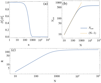
Figure 2: (a) The relative correlation strength $D^{2}_{n}/D^{2}_{0}$ decays with distance $n$, yielding the correlation length $N_{c}\approx 380$. (b) The change of $N_{cor}$ with the number of measurements $N$. When $N\ll N_{c}$, $N_{cor}$ increases linearly (denoted by the orange dashed line). When $N\gg N_{c}$, $N_{cor}$ saturates to a fixed value $N_{s}\approx 640$. (c) The enhancement factor $R$ as a function of $N$. Here, an Ohmic noise spectrum $J(\omega)=\alpha\omega e^{-\omega/\omega_{c}}$ is taken for low-frequency noise. Parameters are: $\alpha=0.1$, $\omega_{c}=10.0$, $\omega_{c}t_{2}=1$, and $\hbar\beta\omega_{c}/t_{2}=10^{3}$.

IV estimation precision for the sequential measurement

Choosing $\theta=\pi/2$, we concentrate on the enhancement of the estimation precision by correlations between different measurements. By setting $t=t_{2}$, the Fisher information is calculated according to the Eq. (2). The QSNR is then determined from the Cramér-Rao bound, given by

$$(\beta/\Delta\beta)^{2}_{cor}\leq 2e^{-4}g^{4}t^{4}_{2}NN_{cor},$$ (11)

where $N_{cor}\equiv\frac{2}{N}\sum_{i<j}D^{2}_{j-i}/D^{2}_{0}$ and the equality $\beta D_{0}=g^{2}t^{2}_{2}/2$ is used. Here, $D^{2}_{j-i}/D^{2}_{0}$ quantifies the relative strength of correlation between $i$-th and $j$ -th measurements in the sequence, which is a decay function of $j-i$. The correlation length $N_{c}$ can be defined from the condition $D^{2}_{n}/D^{2}_{0}=e^{-1}$, beyond which the correlation effect can be safely ignored.

When $N\ll N_{c}$, $N_{cor}\approx(N-1)$, which results in a scaling of $N^{2}$ of the QSNR from Eq. (11)

$$(\beta/\Delta\beta)^{2}_{cor}\leq 2e^{-4}g^{4}t^{2}_{4}N(N-1).$$ (12)

In the low-temperature case, the condition $N_{c}\sim\hbar\beta/t_{2}\gg 1$ suggests that the Heisenberg scaling holds for a wide range of measurement counts $N$. In contrast, when $N\gg N_{c}$, $N_{cor}$ would saturate to a fixed value $N_{s}\propto N_{c}$, which yields an $N$ scaling of the QSNR, given by

$$(\beta/\Delta\beta)^{2}_{cor}\leq 2e^{-4}g^{4}t^{4}_{2}NN_{s}.$$ (13)

However, the property $N_{s}\propto N_{c}\sim\hbar\beta/t_{2}$ indicates that a large enhancement can be expected for low-temperature estimation. We can owe this improvement to the increase in the correlation time in the two-point correlation function $\langle\{\hat{X}(\tau),\hat{X}(\tau^{\prime})\}\rangle_{B}$, which changes from $t_{2}$ for independent measurements to $N_{s}t_{2}$ for sequential measurements, resulting in $\mathcal{F}_{\beta}\sim g^{4}t^{2}_{2}(N_{s}t_{2})^{2}\frac{N}{N_{s}}$.

To reflect the enhancement of the measurement precision induced by the sequential measurements, we introduce an enhancement factor

$$R\equiv(\Delta\beta)^{2}_{ind}/(\Delta\beta)^{2}_{cor}.$$ (14)

Assuming that the Cramér-Rao bound is saturated, one can find that the enhancement factor $R$ increases from $2(e^{-2}-e^{-4})(N-1)$ to $2(e^{-2}-e^{-4})N_{s}$ as $N$ increases.

To elucidate the advantage of sequential measurements, we consider the case where low-frequency noise has Ohmic spectral $J(\omega)=\alpha\omega e^{-\omega/\omega_{c}}$ and temperature-independent noise is ignored. The results are illustrated in Fig. 2 with the parameters $\hbar\beta/t_{2}=10^{3}$. From Fig. 2 (a), one can observe that when $n$ is small, the relative correlation strength $D^{2}_{n}/D^{2}_{0}$ is almost constant, while it decays to zero when $n$ is large enough. Consequently, when $N$ is small, a linear increase of $N_{cor}$ is observed in Fig. 2 (b), which saturates to a fixed value $\sim\hbar\beta/t_{2}$ when $N$ is large enough. In correspondence, the enhancement factor shows a linear increase for the case of small $N$, while it saturates to a fixed value $\sim\hbar\beta/t_{2}$ in the limit of large $N$ .

V Quantum spectroscopy

One can find that that temperature estimation process is equivalent to measuring the noise spectrum of $\hat{X}(\tau)$. To illustrate this equivalence relation, consider the pair correlation in sequential measurements with the setting $\theta=\pi/2$. The mean value of these pairwise outputs, defined as $S_{j,i}\equiv\langle s_{j}s_{i}\rangle-\langle s_{j}\rangle\langle s_{i}\rangle$, are obtained by using the explicit expression of $P_{\bm{S}}$ . The result is

$$S_{j,i}\approx 4t^{2}e^{-2t/t_{2}}C^{++}_{j,i}$$ (15)

One can find that $S_{j,i}$ is directly proportional to the two-point correlation function $C^{++}_{j,i}$. After the Fourier transformation of $S_{j,i}$, the noise spectrum is obtained. Thus, the pair correlation corresponds exactly to the noise spectrum up to a factor $4t^{2}e^{-2t/t_{2}}$.

Note that the spectral resolution obtained from this method is independent of the probe’s (thermometer’s) coherence time, thus facilitating high-resolution spectroscopy [48]. These results differ significantly from the noise spectrum obtained by independent measurements, where only $C^{++}_{i,i}$ is accessed, thereby limiting the resolution to the sensor’s coherence time $1/t_{2}$. This advantage makes sequential measurements desirable for high-resolution quantum spectroscopy [50]. Here, we use sequential measurements to improve the precision of temperature estimation. Because both the correlation functions $C^{++}_{i,i}$ and $C^{++}_{j,i}$ contain temperature information, sequential measurements produce better performance than independent measurements by taking into account all long-term correlations. Hence, both quantum thermometry and high-resolution quantum spectroscopy use sequential measurements to increase the correlation time of the noise in a sample, thereby improving the estimation precision or spectral resolution.

VI conclusions

In this paper, we introduce the sequential measurement to low-temperature thermometry. We show that sequential measurement significantly improves measurement precision in the ultracold scenario with $\hbar\beta/t_{2}\gg 1$. This enhancement stems from the accounting of long-term correlations of low-frequency noise in the thermal sample. A Heisenberg scaling is verified, which holds for a wide range of measurement numbers $N$ in the ultracold scenario with $\hbar\beta/t_{2}\gg 1$. In contrast, a fundamental limit of the estimation precision is reached when $N$ is large enough, determined by the intrinsic correlation time of the low-frequency noise mode. Additionally, we establish a close link between low-temperature quantum thermometry via sequential measurement and quantum correlation spectroscopy. Both of them use sequential measurements to increase the correlation time of the noise in a sample. Noting that temperature is a statistical quantity, our work opens the door to precision measurement of statistical quantities through correlation measurements.

VII Acknowledgment

N. Z. is supported by the National Natural Science Foundation of China (Grant No. 12247101), the Fundamental Research Funds for Central Universities (Grant No. lzujbky-2024-jdzx06) P. W. is supported by the National Natural Science Foundation of China(Grant No. 1247050444), the Talents Introduction Foundation of Beijing Normal University (Grant No. 310432106), Innovation Program for Quantum Science and Technology of China (Project 2023ZD0300600) and Guangdong Provincial Quantum Science Strategic Initiative (Grant No. GDZX2303005).

Appendix A evolution probability $\mathcal{G}(\eta,\bar{\eta})$

In terms of the basis of the z direction $\{|0\rangle,|1\rangle\}$, the measurement operator along the $\theta$-direction reads

$$\hat{\Pi}_{\theta;s}=\frac{1}{2}\sum^{0,1}_{\eta,\bar{\eta}}e^{i\eta^{-}(\theta+\frac{1-s}{2}\pi)}|\eta_{z}\rangle\langle\bar{\eta}_{z}|,$$

where $\eta^{\pm}=(\eta_{i}+\frac{1}{2})\pm(\bar{\eta}_{i}+\frac{1}{2})$. Using this expression, one can get that

$$\mathcal{M}_{s_{j}}\rho_{B}= \sum^{\pm}_{\eta,\bar{\eta}}\frac{1}{4}e^{i\eta^{-}_{j}(\theta+\frac{1-s_{j}}{2}\pi)}\mathcal{T}e^{-\frac{i}{\hbar}(2\eta_{j}-1)\int^{jt}_{(j-1)t}d\tau\hat{X}(\tau)}$$

$$\rho_{B}\bar{\mathcal{T}}e^{\frac{i}{\hbar}(2\bar{\eta}_{j}-1)\int^{jt}_{(j-1)t}d\tau\hat{X}(\tau)},$$ (16)

where $\mathcal{T}$ and $\bar{\mathcal{T}}$ denotes the time-ordering and anti-time-ordering. Based on this result, one can get that

$$P_{\bm{S}}= \frac{1}{4^{N}}\sum_{\bm{\eta},\bar{\bm{\eta}}}e^{i\sum_{j}\eta^{-}_{j}(\theta+\frac{1-s_{j}}{2}\pi)}\mathcal{G}(\bm{\eta},\bar{\bm{\eta}}),$$ (17)

$$\mathcal{G}= \langle\bar{\mathcal{T}}e^{\frac{i}{\hbar}\int^{Nt}_{0}d\tau\hat{X}(\tau)\bar{\eta}^{\prime}(\tau)}\mathcal{T}e^{-\frac{i}{\hbar}\int^{Nt}_{0}d\tau\hat{X}(\tau)\eta^{\prime}(\tau)}\rangle_{B},$$ (18)

where $\bm{\eta}=\{\eta_{i}\}$, $\bar{\bm{\eta}}=\{\bar{\eta}_{i}\}$ and $\eta^{\prime}_{j}(\tau)\equiv 2\eta_{j}-1$, $\bar{\eta}^{\prime}_{j}(\tau)\equiv 2\bar{\eta}_{j}-1$ with $i=\tau/t$. Here, $\mathcal{G}(\bm{\eta},\bar{\bm{\eta}})$ denotes the evolution ”probability” along the path $\bm{\eta}$ and $\bar{\bm{\eta}}$. For Gaussian noise, the average can be exactly solved and the result is

$$\mathcal{G}(\bm{\eta},\bar{\bm{\eta}})= e^{-\frac{1}{\hbar^{2}}\int^{Nt}_{0}d\tau_{1}\int^{t}_{\tau_{1}}d\tau_{2}\bar{\eta}^{\prime}(\tau_{1})\bar{\eta}^{\prime}(\tau_{2})\langle\hat{X}(\tau_{1})\hat{X}(\tau_{2})\rangle_{B}}$$

$$e^{-\frac{1}{\hbar^{2}}\int^{Nt}_{0}d\tau_{1}\int^{\tau_{1}}_{0}d\tau_{2}\eta^{\prime}(\tau_{1})\eta^{\prime}(\tau_{2})\langle\hat{X}(\tau_{1})\hat{X}(\tau_{2})\rangle_{B}}$$

$$e^{\frac{1}{\hbar^{2}}\int^{Nt}_{0}d\tau_{1}\int^{Nt}_{0}d\tau_{2}\bar{\eta}^{\prime}(\tau_{1})\eta^{\prime}(\tau_{2})\langle\hat{X}(\tau_{1})\hat{X}(\tau_{2})\rangle_{B}}.$$ (19)

Using the decomposition $\eta^{\prime}(\tau)=\eta^{+}(\tau)+\eta^{-}(\tau)$ and $\bar{\eta}^{\prime}(\tau)=\eta^{+}(\tau)-\eta^{-}(\tau)$, one can get that

$$\mathcal{G}(\bm{\eta},\bar{\bm{\eta}})= e^{-\frac{2}{\hbar^{2}}\int^{Nt}_{0}d\tau_{1}\int^{\tau_{1}}_{0}d\tau_{2}\eta^{-}(\tau_{1})\eta^{+}(\tau_{2})\langle[\hat{X}(\tau_{1}),\hat{X}(\tau_{2})]\rangle_{B}}$$

$$e^{-\frac{2}{\hbar^{2}}\int^{Nt}_{0}d\tau_{1}\int^{Nt}_{0}d\tau_{2}\eta^{-}(\tau_{1})\eta^{-}(\tau_{2})\langle\{\hat{X}(\tau_{1}),\hat{X}(\tau_{2})\}\rangle_{B}},$$ (20)

where $[\hat{A},\hat{B}]=\hat{A}\hat{B}-\hat{B}\hat{A}$ and $\{\hat{A},\hat{B}\}=(\hat{A}\hat{B}+\hat{B}\hat{A})/2$.

Appendix B probability distribution

By using the noise decomposition $\hat{X}(t)=\hat{X}_{L}(t)+\hat{X}_{H}(t)$ with the assumption $\langle\hat{X}_{H}(t)\hat{X}_{H}(t^{\prime})\rangle_{B}=\frac{1}{t_{2}}\delta(t-t^{\prime})$, the propagator $\mathcal{G}(\bm{\eta},\bar{\bm{\eta}})$ can be expressed as

$$\mathcal{G}=e^{-\sum_{j,l}[2C^{++}_{l,j}\eta^{-}_{l}\eta^{-}_{j}+2iC^{+-}_{l,j}\eta^{-}_{l}\eta^{+}_{j}]-\sum_{j}(\eta^{-}_{j})^{2}\frac{t}{t_{2}}}.$$ (21)

To decouple these two terms, we introduce an effective expression of $\eta^{+}$ as $\eta^{+}\equiv(1-(\eta^{-})^{2})\sigma$ with $\sigma=\pm 1$. One can check that $\eta^{-}$ and $\sigma$ are independent of each other. Using this result, the probability distribution $P_{\bm{S}}$ is reduced to

$$P_{\bm{S}}=\sum_{\bm{\eta}^{-}}\sum_{\bm{\sigma}}\frac{1}{2^{N}}\mathcal{G}(\bm{\eta}^{-},\bm{\sigma})\prod_{j}\frac{e^{i\eta^{-}_{j}(\theta+\frac{1-s_{j}}{2}\pi)}}{4}.$$ (22)

Because the factor $\frac{e^{i\eta^{-}_{j}(\theta+\frac{1-s_{j}}{2}\pi)}}{4}$ is independent of $\sigma_{j}$, the average of $\mathcal{G}$ over $\{\sigma_{j}\}$ with probability $p_{\sigma_{j}=\pm}=1/2$ yields

$$\langle\mathcal{G}\rangle_{\bm{\sigma}}= e^{-2\sum_{j,l}C^{++}_{l,j}\eta^{-}_{l}\eta^{-}_{j}-\sum_{j}\frac{(\eta^{-}_{j})^{2}t}{t_{2}}}$$

$$\prod_{j}\cos(2\sum_{l}C^{+-}_{l,j}\eta^{-}_{l}\mathcal{P}_{j}),$$ (23)

where $\mathcal{P}_{j}=(1-(\eta^{-}_{j})^{2})$. Noting further that $|C^{+-}_{l,j}|\ll 1$, one can get that

$$\langle\mathcal{G}\rangle_{\bm{\sigma}}\approx e^{-2\sum_{j,l}C^{++}_{l,j}\eta^{-}_{l}\Delta\eta_{j}-2\sum_{j}[\sum_{l}C^{+-}_{l,j}\eta^{-}_{l}]^{2}\mathcal{P}_{j}-\sum_{j}\frac{(\eta^{-}_{j})^{2}t}{t_{2}}}$$

$$\approx e^{-2\sum_{j,l}C^{++}_{l,j}\eta^{-}_{l}\eta^{-}_{j}-2\sum_{j}[\sum_{l}C^{+-}_{l,j}\eta^{-}_{l}]^{2}-\sum_{j}(\eta^{-}_{j})^{2}\frac{t}{t_{2}}}.$$

In the last step, we use the fact that $2(\sum_{l}C^{+-}_{l,j}\eta^{-})^{2}\ll t/t_{2}$. A further simplification yields that

$$\langle\mathcal{G}\rangle_{\bm{\sigma}}\approx e^{-\sum_{l,l^{\prime}}2[C^{++}_{l,l^{\prime}}+\sum_{j}C^{+-}_{l,j}C^{+-}_{l^{\prime},j}]\eta^{-}_{l}\eta^{-}_{l^{\prime}}-\sum_{l}(\eta^{-}_{l})^{2}\frac{t}{t_{2}}}.$$ (24)

To solve the distribution function $P_{\bm{S}}$, we introduce an auxiliary field decomposition of $\langle\mathcal{G}\rangle_{\bm{\sigma}}$, given by

$$e^{-\sum_{l,l^{\prime}}\eta^{-}_{l}D_{l,l^{\prime}}\eta^{-}_{l^{\prime}}}= \frac{1}{\sqrt{\det[\pi D]}}\int\prod_{j}d\phi_{j}$$

$$e^{-\sum_{l,l^{\prime}}\phi_{l}D^{-1}_{l,l^{\prime}}\phi_{l^{\prime}}+i2\sum_{l}\phi_{l}\eta^{-}_{l}},$$

where $\phi_{l}$ is denoted as the auxiliary field. The result is then reduced to

$$P_{\bm{S}}=\langle\prod_{j}[\frac{1}{2}+\frac{s_{j}}{2}\cos(2\phi_{j}+\theta)]\rangle_{\bm{\phi}},$$ (25)

where $\langle\rangle_{\bm{\phi}}$ denotes the average over the auxilliary fields$\{\phi_{j}\}$ with given distribution function $P_{\bm{\phi}}=\frac{e^{-\sum_{l,l^{\prime}}\phi_{l}D^{-1}_{l,l^{\prime}}\phi_{l^{\prime}}}}{\sqrt{\det[\pi D]}}$ with $D_{l,l^{\prime}}=\delta_{l,l^{\prime}}\frac{t}{t_{2}}+2C^{++}_{l,l^{\prime}}+2\sum_{j}C^{+-}_{l,j}C^{+-}_{l^{\prime},j}$.

By considering the weak correlation between different auxiliary fields $\{\phi_{l}\}$ , the distribution function $P_{\bm{S}}$ can be approximated as

$$P_{\bm{S}}\approx\prod_{l}P_{s_{l}}\prod_{l^{\prime}<l}\frac{P_{s_{l},s_{l}^{\prime}}}{P_{s_{l}}P_{s_{l}^{\prime}}},$$ (26)

where $P_{s_{l}}=\langle[\frac{1}{2}+\frac{s_{l}}{2}\cos(2\phi_{l}+\theta)]\rangle_{\bm{\phi}}$ and $P_{s_{l},s_{l}^{\prime}}=\langle[\frac{1}{2}+\frac{s_{l}}{2}\cos(2\phi_{l}+\theta)][\frac{1}{2}+\frac{s_{l}^{\prime}}{2}\cos(2\phi_{l}^{\prime}+\theta)]\rangle_{\bm{\phi}}$. By further noting that $\langle\cos(2\phi_{l}+\theta)\rangle_{\bm{\phi}}=\cos\theta e^{-D_{l,l}}$ and $\langle\cos(2\phi_{l}+\theta)\cos(2\phi_{l^{\prime}}+\theta)\rangle_{\bm{\phi}}=e^{-D_{l,l}-D_{l^{\prime},l^{\prime}}}[\cos^{2}\theta\cosh(D_{l,l^{\prime}}+D_{l^{\prime},l})+\sin^{2}\theta\sinh(D_{l,l^{\prime}}-D_{l^{\prime},l})]$, one can get that

$$P_{\bm{S}}\approx \prod_{l}P_{s_{l}}\prod_{l^{\prime}<l}[1+s_{l}s_{l^{\prime}}T_{l,l^{\prime}}],$$

$$T_{l,l^{\prime}}\equiv \frac{\cos^{2}\theta\sinh^{2}D_{l,l^{\prime}}-\sin^{2}\theta(1-\sinh{2D_{l,l^{\prime}}})}{4P_{s_{l}}P_{s_{l}^{\prime}}}e^{-D_{l,l}-D_{l^{\prime},l^{\prime}}},$$

where $D_{l,l^{\prime}}=D_{l^{\prime},l}$ is used. By further ignoring high-order of $C^{+\pm}_{l,l^{\prime}}$, the final result is then simplified to

$$P_{\bm{S}}\approx\prod_{l}P_{s_{l}}\prod_{l^{\prime}<l}[1-s_{l}s_{l^{\prime}}\frac{\sin^{2}\theta C^{++}_{l,l^{\prime}}}{P_{s_{l}}P_{s_{l}^{\prime}}}e^{-2t/t_{2}}],$$ (27)

where $P_{s_{l}}\approx\frac{1}{2}+\frac{s_{l}}{2}\cos\theta e^{-t/t_{2}-C^{++}_{l,l}}$.

References

- Gross and Bloch [2017] C. Gross and I. Bloch, Quantum simulations with ultracold atoms in optical lattices, Science 357, 995 (2017).
- Browaeys and Lahaye [2020] A. Browaeys and T. Lahaye, Many-body physics with individually controlled rydberg atoms, Nat. Phys. 16, 132 (2020).
- Ebadi et al. [2021] S. Ebadi, T. T. Wang, H. Levine, A. Keesling, G. Semeghini, A. Omran, D. Bluvstein, R. Samajdar, H. Pichler, W. W. Ho, S. Choi, S. Sachdev, M. Greiner, V. Vuletić, and M. D. Lukin, Quantum phases of matter on a 256-atom programmable quantum simulator, Nature 595, 227 (2021).
- Morgado and Whitlock [2021] M. Morgado and S. Whitlock, Quantum simulation and computing with Rydberg-interacting qubits, AVS Quantum Science 3, 023501 (2021).
- Leanhardt et al. [2003] A. E. Leanhardt, T. A. Pasquini, M. Saba, A. Schirotzek, Y. Shin, D. Kielpinski, D. E. Pritchard, and W. Ketterle, Cooling bose-einstein condensates below 500 picokelvin, Science 301, 1513 (2003).
- Gati et al. [2006] R. Gati, B. Hemmerling, J. Fölling, M. Albiez, and M. K. Oberthaler, Noise thermometry with two weakly coupled bose-einstein condensates, Phys. Rev. Lett. 96, 130404 (2006).
- Correa et al. [2017] L. A. Correa, M. Perarnau-Llobet, K. V. Hovhannisyan, S. Hernández-Santana, M. Mehboudi, and A. Sanpera, Enhancement of low-temperature thermometry by strong coupling, Phys. Rev. A 96, 062103 (2017).
- Mehboudi et al. [2019a] M. Mehboudi, A. Lampo, C. Charalambous, L. A. Correa, M. A. García-March, and M. Lewenstein, Using polarons for sub-nk quantum nondemolition thermometry in a bose-einstein condensate, Phys. Rev. Lett. 122, 030403 (2019a).
- Mitchison et al. [2020] M. T. Mitchison, T. Fogarty, G. Guarnieri, S. Campbell, T. Busch, and J. Goold, In situ thermometry of a cold fermi gas via dephasing impurities, Phys. Rev. Lett. 125, 080402 (2020).
- Bouton et al. [2020] Q. Bouton, J. Nettersheim, D. Adam, F. Schmidt, D. Mayer, T. Lausch, E. Tiemann, and A. Widera, Single-atom quantum probes for ultracold gases boosted by nonequilibrium spin dynamics, Phys. Rev. X 10, 011018 (2020).
- Adam et al. [2022] D. Adam, Q. Bouton, J. Nettersheim, S. Burgardt, and A. Widera, Coherent and dephasing spectroscopy for single-impurity probing of an ultracold bath, Phys. Rev. Lett. 129, 120404 (2022).
- Stace [2010] T. M. Stace, Quantum limits of thermometry, Phys. Rev. A 82, 011611 (2010).
- Johnson et al. [2016] T. H. Johnson, F. Cosco, M. T. Mitchison, D. Jaksch, and S. R. Clark, Thermometry of ultracold atoms via nonequilibrium work distributions, Phys. Rev. A 93, 053619 (2016).
- Razavian et al. [2019] S. Razavian, C. Benedetti, M. Bina, Y. Akbari-Kourbolagh, and M. G. A. Paris, Quantum thermometry by single-qubit dephasing, Eur. Phys. J. Plus 134, 284 (2019).
- Yuan et al. [2023] J.-B. Yuan, B. Zhang, Y.-J. Song, S.-Q. Tang, X.-W. Wang, and L.-M. Kuang, Quantum sensing of temperature close to absolute zero in a bose-einstein condensate, Phys. Rev. A 107, 063317 (2023).
- Mehboudi et al. [2019b] M. Mehboudi, A. Sanpera, and L. A. Correa, Thermometry in the quantum regime: recent theoretical progress, J. Phys. A 52, 303001 (2019b).
- Potts et al. [2019] P. P. Potts, J. B. Brask, and N. Brunner, Fundamental limits on low-temperature quantum thermometry with finite resolution, Quantum 3, 161 (2019).
- Jørgensen et al. [2020] M. R. Jørgensen, P. P. Potts, M. G. A. Paris, and J. B. Brask, Tight bound on finite-resolution quantum thermometry at low temperatures, Phys. Rev. Res. 2, 033394 (2020).
- Mihailescu et al. [2023] G. Mihailescu, S. Campbell, and A. K. Mitchell, Thermometry of strongly correlated fermionic quantum systems using impurity probes, Phys. Rev. A 107, 042614 (2023).
- Brenes and Segal [2023] M. Brenes and D. Segal, Multispin probes for thermometry in the strong-coupling regime, Phys. Rev. A 108, 032220 (2023).
- Seah et al. [2019] S. Seah, S. Nimmrichter, D. Grimmer, J. P. Santos, V. Scarani, and G. T. Landi, Collisional quantum thermometry, Phys. Rev. Lett. 123, 180602 (2019).
- Alves and Landi [2022] G. O. Alves and G. T. Landi, Bayesian estimation for collisional thermometry, Phys. Rev. A 105, 012212 (2022).
- Hovhannisyan and Correa [2018] K. V. Hovhannisyan and L. A. Correa, Measuring the temperature of cold many-body quantum systems, Phys. Rev. B 98, 045101 (2018).
- Mirkhalaf et al. [2021] S. S. Mirkhalaf, D. Benedicto Orenes, M. W. Mitchell, and E. Witkowska, Criticality-enhanced quantum sensing in ferromagnetic bose-einstein condensates: Role of readout measurement and detection noise, Phys. Rev. A 103, 023317 (2021).
- Aybar et al. [2022] E. Aybar, A. Niezgoda, S. S. Mirkhalaf, M. W. Mitchell, D. Benedicto Orenes, and E. Witkowska, Critical quantum thermometry and its feasibility in spin systems, Quantum 6, 808 (2022).
- Zhang et al. [2022] N. Zhang, C. Chen, S.-Y. Bai, W. Wu, and J.-H. An, Non-markovian quantum thermometry, Phys. Rev. Appl. 17, 034073 (2022).
- Zhang and Wu [2021] Z.-Z. Zhang and W. Wu, Non-markovian temperature sensing, Phys. Rev. Res. 3, 043039 (2021).
- Xu et al. [2023] L. Xu, J.-B. Yuan, S.-Q. Tang, W. Wu, Q.-S. Tan, and L.-M. Kuang, Non-markovian enhanced temperature sensing in a dipolar bose-einstein condensate, Phys. Rev. A 108, 022608 (2023).
- Zhang et al. [2024] N. Zhang, S.-Y. Bai, and C. Chen, Temperature-heat uncertainty relation in nonequilibrium quantum thermometry, Phys. Rev. A 110, 012211 (2024).
- Planella et al. [2022] G. Planella, M. F. B. Cenni, A. Acín, and M. Mehboudi, Bath-induced correlations enhance thermometry precision at low temperatures, Phys. Rev. Lett. 128, 040502 (2022).
- Brattegard and Mitchison [2024] S. Brattegard and M. T. Mitchison, Thermometry by correlated dephasing of impurities in a one-dimensional fermi gas, Phys. Rev. A 109, 023309 (2024).
- [32] N. Zhang and C. Chen, Achieving heisenberg scaling in low-temperature quantum thermometry, arXiv:2407.05762 .
- Burgarth et al. [2015] D. Burgarth, V. Giovannetti, A. N. Kato, and K. Yuasa, Quantum estimation via sequential measurements, New J. Phys. 17, 113055 (2015).
- De Pasquale et al. [2017] A. De Pasquale, K. Yuasa, and V. Giovannetti, Estimating temperature via sequential measurements, Phys. Rev. A 96, 012316 (2017).
- Montenegro et al. [2022] V. Montenegro, G. S. Jones, S. Bose, and A. Bayat, Sequential measurements for quantum-enhanced magnetometry in spin chain probes, Phys. Rev. Lett. 129, 120503 (2022).
- Radaelli et al. [2023] M. Radaelli, G. T. Landi, K. Modi, and F. C. Binder, Fisher information of correlated stochastic processes, New J. Phys. 25, 053037 (2023).
- Giovannetti et al. [2006] V. Giovannetti, S. Lloyd, and L. Maccone, Quantum metrology, Phys. Rev. Lett. 96, 010401 (2006).
- Giovannetti et al. [2011] V. Giovannetti, S. Lloyd, and L. Maccone, Advances in quantum metrology, Nat. Photonics 5, 222 (2011).
- Braun et al. [2018] D. Braun, G. Adesso, F. Benatti, R. Floreanini, U. Marzolino, M. W. Mitchell, and S. Pirandola, Quantum-enhanced measurements without entanglement, Rev. Mod. Phys. 90, 035006 (2018).
- Wang et al. [2019] P. Wang, C. Chen, X. Peng, J. Wrachtrup, and R.-B. Liu, Characterization of arbitrary-order correlations in quantum baths by weak measurement, Phys. Rev. Lett. 123, 050603 (2019).
- Wang et al. [2021] P. Wang, C. Chen, and R.-B. Liu, Classical-noise-free sensing based on quantum correlation measurement, Chin. Phys. Lett. 38, 010301 (2021).
- Wu et al. [2024] Z. Wu, P. Wang, T. Wang, Y. Li, R. Liu, Y. Chen, X. Peng, and R.-B. Liu, Selective detection of dynamics-complete set of correlations via quantum channels, Phys. Rev. Lett. 132, 200802 (2024).
- [43] B. C. H. Cheung and R.-B. Liu, Quantum nonlinear spectroscopy via correlations of weak faraday-rotation measurements, Adv. Quantum Technol. , 2300286.
- Meinel et al. [2022] J. Meinel, V. Vorobyov, P. Wang, B. Yavkin, M. Pfender, H. Sumiya, S. Onoda, J. Isoya, R.-B. Liu, and J. Wrachtrup, Quantum nonlinear spectroscopy of single nuclear spins, Nat. Commun. 13, 5318 (2022).
- Shen et al. [2023] Y. Shen, P. Wang, C. T. Cheung, J. Wrachtrup, R.-B. Liu, and S. Yang, Detection of quantum signals free of classical noise via quantum correlation, Phys. Rev. Lett. 130, 070802 (2023).
- Laraoui et al. [2013] A. Laraoui, F. Dolde, C. Burk, F. Reinhard, J. Wrachtrup, and C. A. Meriles, High-resolution correlation spectroscopy of 13c spins near a nitrogen-vacancy centre in diamond, Nat. Commun. 4, 1651 (2013).
- Aslam et al. [2017] N. Aslam, M. Pfender, P. Neumann, R. Reuter, A. Zappe, F. F. de Oliveira, A. Denisenko, H. Sumiya, S. Onoda, J. Isoya, and J. Wrachtrup, Nanoscale nuclear magnetic resonance with chemical resolution, Science 357, 67 (2017).
- Boss et al. [2017] J. M. Boss, K. S. Cujia, J. Zopes, and C. L. Degen, Quantum sensing with arbitrary frequency resolution, Science 356, 837 (2017).
- Glenn et al. [2018] D. R. Glenn, D. B. Bucher, J. Lee, M. D. Lukin, H. Park, and R. L. Walsworth, High-resolution magnetic resonance spectroscopy using a solid-state spin sensor, Nature 555, 351 (2018).
- Pfender et al. [2019] M. Pfender, P. Wang, H. Sumiya, S. Onoda, W. Yang, D. B. R. Dasari, P. Neumann, X.-Y. Pan, J. Isoya, R.-B. Liu, and J. Wrachtrup, High-resolution spectroscopy of single nuclear spins via sequential weak measurements, Nat. Commun. 10, 594 (2019).
- Cujia et al. [2019] K. S. Cujia, J. M. Boss, K. Herb, J. Zopes, and C. L. Degen, Tracking the precession of single nuclear spins by weak measurements, Nature 571, 230 (2019).
- Kovachy et al. [2015] T. Kovachy, J. M. Hogan, A. Sugarbaker, S. M. Dickerson, C. A. Donnelly, C. Overstreet, and M. A. Kasevich, Matter wave lensing to picokelvin temperatures, Phys. Rev. Lett. 114, 143004 (2015).
- Breuer and Petruccione [2007] H.-P. Breuer and F. Petruccione, The Theory of Open Quantum Systems (Oxford University Press, 2007).
- Degen et al. [2017] C. L. Degen, F. Reinhard, and P. Cappellaro, Quantum sensing, Rev. Mod. Phys. 89, 035002 (2017).