Sequential anomaly identification with observation control under generalized error metrics
Abstract
The problem of sequential anomaly detection and identification is considered, where multiple data sources are simultaneously monitored and the goal is to identify in real time those, if any, that exhibit “anomalous” statistical behavior. An upper bound is postulated on the number of data sources that can be sampled at each sampling instant, but the decision maker selects which ones to sample based on the already collected data. Thus, in this context, a policy consists not only of a stopping rule and a decision rule that determine when sampling should be terminated and which sources to identify as anomalous upon stopping, but also of a sampling rule that determines which sources to sample at each time instant subject to the sampling constraint. Two distinct formulations are considered, which require control of different, “generalized” error metrics. The first one tolerates a certain user-specified number of errors, of any kind, whereas the second tolerates distinct, user-specified numbers of false positives and false negatives. For each of them, a universal asymptotic lower bound on the expected time for stopping is established as the error probabilities go to 0, and it shown to be attained by a policy that combines the stopping and decision rules proposed in the full-sampling case with a probabilistic sampling rule that achieves a specific long-run sampling frequency for each source. Moreover, the optimal to a first-order asymptotic approximation expected time for stopping is compared in simulation studies with the corresponding factor in a finite regime, and the impact of the sampling constraint and tolerance to errors is assessed.
Index Terms:
Anomaly identification, generalized error metric, sampling design, asymptotic optimality.I Introduction
In many scientific and engineering applications, measurements from various data sources are collected sequentially, aiming to identify in real-time the sources, if any, with “anomalous” statistical behavior. In internet security systems [2], for example, the data streams may refer to the transition rate of a link, where a meager rate warns of a possible intrusion. In finance, the data streams may refer to prices in the stock market [3], where we need to detect an unusual rate of return of a stock price.
Such applications, among many others, motivate the formulation of sequential multiple testing problems where multiple data sources are monitored sequentially, a binary hypothesis testing problem is formulated for each of them, and the goal is to simultaneously solve these testing problems as quickly as possible, while controlling certain error metrics. In some works, e.g.,[4, 5, 6], it is assumed that all sources can be monitored at each sampling instant upon stopping. In others, e.g., [7, 8, 9, 10, 11, 12, 13, 14, 15], a sampling constraint is imposed, according to which it is possible to observe only a subset of sources at each time instant, but the decision maker selects which ones to sample based on the already collected data. In the latter case, in addition to a stopping rule and a decision rule that determine when to stop sampling and which sources to identify as anomalous upon stopping, it is also required to specify a sampling rule, which determines the sources to be sampled at each time instant until stopping. This sampling constraint leads to a sequential multiple testing problem with adaptive sampling design, which lies in the field of “sequential testing with controlled sensing”, or “sequential design of experiments” [16], [17], [18], [19]. Hence, methods and results from these works are applicable as well.
In the above works, the problem formulation requires, implicitly or explicitly, control of the “classical” misclassification error rate, i.e., the probability of at least one error, of any kind, or of the two “classical” familywise error rates, i.e., the probabilities of at least one false alarm and at least one missed detection. However, such error metrics can be impractical, especially when there is a common stopping time at which the decision is made for all data sources, as in the above papers. Indeed, even with a relatively small number of data sources, a single “difficult” hypothesis may determine, even inflate, the overall time required for the decisions to be made.
This inflexibility has motivated the adoption of more lenient error metrics, which are prevalent in the fixed-sample-size literature of multiple testing [20, 21, 22]. As it was shown in [22], the methodology and asymptotic optimality theory in [6], [9] for the sequential identification problem under classical familywise error rates remain valid with other error metrics as long as the latter are bounded above and below up to a multiplicative constant by the corresponding classical familywise error rates. 111The authors in [22] focus in the full sampling case, but exactly the same arguments apply in the case of sampling constraints. This is indeed the case for many error metrics, such as the false discovery rate (FDR) and the false non-discovery rate (FNR) [23]. However, it is not the case for others, such as the generalized misclassification error rate, which requires control of the probability of at least errors of any kind, and the generalized familywise type-I and type-II errors [24, 25, 26], which require control of the probabilities of at least false alarms and at least missed detections. As it was shown in [27] in the case of full sampling, that is, when all data sources are continuously monitored and there are no sampling constraints, the sequential identification problem with these generalized error metrics when or requires a distinct methodology and pose additional mathematical challenges compared to their corresponding classical versions, where or .
In the present work, we address the same sequential anomaly identification problem as in [27], but in the presence of sampling constraints. That is, unlike [27], we assume that it is not possible to observe all data sources at all times. Instead, we impose an upper bound on the average number of samples collected from all sources up to stopping. For each of the two resulting problem formulations, i.e., for each of the two generalized error metrics under consideration, (i) we establish a universal lower bound on the optimal expected time for stopping, to a first-order asymptotic approximation as the corresponding error probabilities go to zero, (ii) we show that this lower bound is attained by a policy that utilizes the stopping and decision rules in [27], as long as the long-run sampling frequency of each source is greater than or equal to a certain value, which is computed explicitly and depends both on the source and on the true subset of anomalous sources, (iii) we show that the latter can be achieved by a probabilistic sampling rule.
The methodology and the theory that we develop in the present work is based on an interplay of techniques, ideas, and methods from the sequential multiple testing problem with full sampling and generalized error control in [27], and the sequential multiple testing problem with sampling constraints and “classical” familywise error control in [9]. However, there are various interesting special features that arise in the present work, both from a technical but also from a methodological point of view. First, there are certain technical challenges which force us to strengthen some of our assumptions compared to [9]. Specifically, we require a stronger moment assumption on the log-likelihood ratio statistics than the finiteness of the Kullback-Leibler information numbers, and we have to postulate a harder sampling constraint (which is still weaker than the usual constraint in the literature that fixes the number of sources that are sampled at each time instant). Second, while in [9] it is shown that there is no need for “forced exploration”, as in the general sequential testing problem with controlled sensing [16, 17], this turns out to be needed in this work.
The remainder of the paper is organized as follows. In Section II, we formulate the two problems we consider in this work. In Section III, we state and solve two auxiliary max-min optimization problems, which play a key role in the formulation of our main results. In Section IV, we state the universal asymptotic lower bound for each of the two problems. In Section V, for each of the two problems, we introduce a family of policies that satisfies the error constraints, and we state a criterion on the sampling rule that guarantees the asymptotic optimality of such a policy. In Section VI, we present a class of probabilistic sampling rules for which the aforementioned criterion is satisfied. In Section VII, we present a simulation study that illustrates our theoretical results, and in Section VIII, we state our conclusions and discuss future research directions.
We end this section with some notations we use throughout the paper. We use to indicate the definition of a new quantity and to indicate the equivalence of two notions. We set , , and for . We denote by the size and by the powerset of a set , and by the symmetric difference of two sets . The , stand for the floor and the ceiling of a positive number . The indicator function is denoted by . In a summation, if the lower limit is larger than the upper limit, then the summation is assumed to be equal to . For positive sequences and , we write when , when , and when . Finally, iid stands for independent and identically distributed.
II Problem formulation
Let be a measurable space and let be a probability space that hosts independent sequences of iid, -valued random elements, , , which are generated by distinct data sources, and independent sequences of random variables, , , uniformly distributed in , to be used for randomization purposes. For each , we assume that each has a density with respect to some -finite measure that is equal to either or , and we say that source is “anomalous” if its density is . We denote by the underlying probability measure, and by the corresponding expectation, when the subset of anomalous sources is . We simply write and whenever the identity of the subset of anomalous sources is not relevant.
The problem we consider is the identification of the anomalous sources, if any, on the basis of sequentially acquired observations from all sources when it is not possible to observe all of them at every sampling instant. Specifically, we have to specify (i) the random time, , at which sampling is terminated, (ii) the subset of sources, , that are declared as anomalous upon stopping, and, for each , (iii) the subset, , of sources that are sampled at time . At any time instant, the decision whether to stop or not, as well as the subsets of sources that are identified as anomalous in the former case, or sampled next in the latter, must be determined based on the already collected data.
Therefore, we say that is a sampling rule if is -measurable for every , where
| (1) |
and . Moreover, we say that the triplet is a policy if
-
(i)
is a sampling rule,
-
(ii)
is a stopping time with respect to filtration ,
-
(iii)
is -measurable, i.e.,
in which case we refer to as a stopping rule and to as a decision rule.
We denote by the family of all policies, and we focus on policies that satisfy a sampling constraint and control the probabilities of certain types of error. To define these, we need to introduce some additional notation. Thus, for any sampling rule and time instant , we denote by the indicator of whether source is sampled at time , i.e.,
by the proportion of times source has been sampled in the first time instants, i.e.,
| (2) |
and we note that the average number of observations from all sources in the first time instants is
| (3) |
II-A The sampling constraint
For any real number in , we say that a policy belongs to if the average number of observations from all sources until stopping is less than or equal to , i.e.,
| (4) |
II-B The error constraints
We consider two types of error control, which lead to two distinct problem formulations. We characterize them both as “generalized”, as they generalize their corresponding “classical” versions of misiclassification error rate and familywise error rates.
II-B1 Control of generalized misclassification error rate
For any , , and , we say that a policy in belongs to if the probability of at least errors of any kind is at most , i.e.,
| (7) |
and we denote by the smallest possible expected time for stopping in , when the subset of anomalous sources is , i.e.,
| (8) |
The first problem we consider in this paper is to evaluate
to a first-order asymptotic approximation as for any , and to find a policy that achieves in this asymptotic sense, simultaneously for every .
II-B2 Control of generalized familywise error rates
For any , , and , such that and , we say that a policy in belongs to if the probability of at least false positives does not exceed and the probability of at least false negatives does not exceed , i.e.,
| (9) |
and we denote by the smallest expected time for stopping in when the subset of anomalous sources is , i.e.,
| (10) |
The second problem we consider in this paper is to evaluate to a first-order asymptotic approximation as , for any , and to find a family of policies that achieves in this asymptotic sense, simultaneously for every .
Remark II.1
As we mentioned in the Introduction, both problems have been solved for the full sampling case, i.e., when all sources are observed at each instant, in [27]. On the other hand, in the presence of sampling constraints, neither of them has been considered beyond the special case of “classical” misclassification error rate () and “classical” familywise error rates () in [9].
II-C Distributional Assumptions
For each , the Kullback-Leibler (KL) divergences of and are assumed to be positive and finite, i.e., for each we have:
| (11) | ||||
To establish asymptotic lower bounds for (8) and (10), we assume that
| (12) | ||||
where . This assumption is not needed neither in the full sampling case considered in [27], nor in the case of classical error control ( or ) under sampling constraints in [9]. Nevertheless, it is weaker than the typical assumption in the sequential controlled sensing literature (e.g.,[16], [17]), according to which it is required that
| (13) | ||||
holds for . However, in order to show that the asymptotic lower bound in (8) and (10) can be achieved, in certain cases we will need to require that (13) holds for some .
III Two max-min optimization problems
In this section, we formulate and solve two auxiliary max-min optimization problems. These will be used in Section IV to express the asymptotic lower bounds for (8) and (10), and in Section V to design procedures that achieve these lower bounds.
To be specific, we denote by an ordered set of positive numbers, i.e.,
| (14) |
for each , we denote by the harmonic mean of the largest elements in , i.e.,
| (15) |
and we also set . Then, assuming that , we introduce the following function,
| (16) |
where
-
•
is a positive integer in ,
-
•
is a vector in
(17)
The constants and are defined as in the previous section, i.e., is a positive integer, and a real number in .
III-A Optimization Problem I
Let be an ordered set of size , and . The first max-min optimization problem we consider is
| (18) |
In the following lemma, we provide an expression for the value of the max-min optimization problem (18), as well as for the maximizer of (18) with the minimum norm.
Lemma III.1
The value of the max-min optimization problem (18) is equal to the expression
| (19) |
where are real numbers in , and are integer numbers in such that . The values of , , , are determined by Algorithm 1 presented in Appendix A. The maximizer of (18) with the minimum norm is given by
| (20) |
where
-
•
for all we have
(21) -
•
if then
(22) -
•
if then
(23) -
•
if then
(24) -
•
if then
(25)
Proof:
Appendix A. ∎
Remark III.1
In the symmetric case where for all , then
and for all .
Remark III.2
Based on the size of we distinguish the following cases on the form of .
-
•
If is relatively large, i.e.,
(26) then
(27) which is the largest possible value that can take over all possible values of . In this case , , .
-
•
If is relatively small, i.e.,
(28) then
where is a quantity defined as
In this case , , , and .
- •
Remark III.3
III-B Optimization Problem II
Let and be two ordered sets such that , let , be two positive integers such that , , and let be an arbitrary positive number. The second max-min optimization problem we consider in this section is more complex than the first, and it has the form
| (30) |
where the function is defined in (16), and , the size of being , and
| (31) | ||||
As we show in the following lemma, the value of the max-min optimization problem (30) is equal to the value of the following optimization problem,
| (32) |
such that the following two constraints hold
| (33) | ||||
Definition III.1
We denote by the maximizer of the constrained optimization problem (32) with the minimum norm, i.e., the minimum sum , among all maximizers. Based on Lemma III.1, we denote by the parameters such that
and by the parameters such that
The parameters , and can be computed by applying Algorithm 1 for each case.
The parameters , and are used in the expression of the maximizers of (30) with the minimum norm.
Lemma III.2
The value of the max-min optimization problem (30) is equal to
| (34) | ||||
The maximizer of (30) with the minimum norm is given by
| (35) |
where
-
•
for all we have
(36) -
•
if then
(37) -
•
if then
(38) -
•
if then
(39) -
•
if then
(40)
and
-
•
for all we have
(41) -
•
if then
(42) -
•
if then
(43) -
•
if then
(44) -
•
if then
(45)
Proof:
Appendix A. ∎
IV Universal asymptotic lower bounds
In this section, we fix an arbitrary , and as in Section II, and we establish a universal asymptotic lower bound for (8) and (10), as , and respectively, under the moment assumption (12).
IV-A The case of generalized misclassification error rate
To state the asymptotic lower bound for as , we need to introduce some additional notation. Thus, we denote by
| (46) |
the ordered set that consists of the Kullback-Leibler numbers in . In particular, for each , is the smallest element in , and can be interpreted as a measure of the difficulty of the most difficult testing problem.
The overall difficulty of the testing problem is determined by the quantity , as described in the following theorem.
Proof:
Appendix B. ∎
Remark IV.1
Consider the homogeneous and symmetric setup where the difficulty is the same across all testing problems, in the sense that
Then, for every we have
Consequently, by Remark III.1 we can see that
IV-B The case of generalized familywise error rates
We next establish an asymptotic lower bound for as and / or . For this, we need to introduce the following notation.
-
(i)
If , for each we denote
-
•
by the smallest element in ,
-
•
by the harmonic mean of the largest elements in .
Moreover, we denote by the ordered set that consists of the Kullback-Leibler numbers in , i.e.,
and for each , we denote by the set that consists of the largest elements in , i.e.,
-
•
-
(ii)
If , for each we denote
-
•
by the smallest element in ,
-
•
by the harmonic mean of the largest elements in .
Moreover, we denote by the ordered set that consists of the Kullback-Leibler numbers in , i.e.,
and for each , we denote by the ordered set that consists of the largest elements in , i.e.,
-
•
We state first the asymptotic lower bound for when and when , as and , respectively.
Theorem IV.2
Proof:
Appendix B.
∎
Remark IV.2
If the sources with the smallest KL numbers in are not considered in the evaluation of the difficulty of the testing problem. This is because we can intentionally misclassify these sources as anomalous without exceeding the tolerance level of false alarm errors in order to reduce the expected stopping time. The respective remark holds for the case .
We continue with the asymptotic lower bound when as so that
| (50) |
For this, we need to introduce the following definition.
Definition IV.1
We denote by the maximum of the following quantities. Each quantity is included to the overall maximum given that the respective condition is satisfied. We recall that or , because otherwise we would have which contradicts the initial assumption .
-
•
If we include the
(51) over all .
-
•
If we include the
(52) over all .
-
•
If we include the
(53) -
•
If we include the
(54)
Remark IV.3
The difficulty of the testing problem is determined by the quantity as described in the following theorem.
Theorem IV.3
Proof:
Appendix B. ∎
We denote by the value of the parameter which corresponds to the maximum of the quantities in Definition IV.1, as it is used in the formulation of the following results.
Definition IV.2
The quantity is defined as follows.
-
•
If is equal to (51), then is the number such that
(60) -
•
If is equal to , then is the number such that
(61) -
•
If is equal to , then .
-
•
If is equal to , then .
Remark IV.4
If is equal to (51), the sources with the smallest KL numbers in are not considered in the evaluation of the difficulty of the testing problem. This is because we can intentionally misclassify these sources as anomalous without exceeding the tolerance level of false alarms in order to reduce the expected stopping time. The respective remark holds if is equal to (52).
If then we can intentionally misclassify as anomalous the sources with the smallest KL numbers in without exceeding the tolerance level of false alarms in order to reduce the expected stopping time. The remaining sources in are already less than the tolerance level of the missed detection errors and this is why the difficulty of the testing problem is determined only by the KL numbers in in (53). The respective remark holds if .
V A criterion for asymptotic optimality
In this section, for each of the two problems under consideration, we first introduce a stopping and a decision rule so that the corresponding error constraint is satisfied for any choice of sampling rule. For this, we adopt the approach in [27], where the full sampling case was considered. Subsequently, we establish the second main result of this paper, which is a criterion on the sampling rule for the resulting policy to achieve the corresponding universal asymptotic lower bound in the previous section.
In what follows, for any sampling rule and for each source , we denote by the local log-likelihood ratio (LLR) of source based on the observations from it in the first time instants, i.e.,
| (62) |
V-A The case of generalized misclassification error
For any sampling rule , we denote by the first time that the sum of the smallest LLRs in absolute value is larger than some threshold , and by the subset of data sources with positive LLRs upon stopping, i.e.,
| (63) | ||||
| (64) |
where, for each and , denotes the smallest LLR in absolute value at time , i.e., the smallest element in . In the full-sampling case, where for every , coincides with the sum-intersection rule, introduced in [27]. Similarly to [27, Theorem 3.1], it can be shown that if the threshold in (63) is selected as
| (65) |
then the policy satisfies the error constraint (7) for any sampling rule . Next, we show that this policy, with this choice of threshold, also achieves the asymptotic lower bound in Theorem IV.1 when, for each , the long-run frequency of the source that corresponds to is not smaller than the quantity , defined according to (20) of Lemma III.1. To be specific, we need the following definition.
Definition V.1
We are now ready to state the first main result of this section.
Theorem V.1
Proof:
Appendix C. ∎
V-B The case of generalized familywise error metric
For any sampling rule , we denote by the number of non-negative LLRs at time , by the indices of the increasingly ordered non-negative LLRs at time , and by the indices of the decreasingly ordered negative LLRs at time , i.e.,
| (69) | ||||
We also set
| (70) | ||||
For any integer such that , we set
| (71) |
Also, for any integer with , we set
| (72) |
We denote by the minimum of the stopping times in (71) and (72), i.e.,
| (73) |
and depending on whether the minimum is attained by a for some , or by a for some , and we set
| (74) |
In the full-sampling case, where for every , coincides with the leap rule, introduced in [27]. Similarly to [27, Theorem 4.1], it can be shown that if the thresholds and in (71)-(72) are selected as
| (75) | ||||
then the policy satisfies the error constraint (9) for any sampling rule . We next show that this policy, with this choice of threshold, achieves the asymptotic lower bound in Theorem IV.3, as long as the long-run sampling frequency of each source is sufficiently large. To be specific, we introduce the following definition, for which we recall the definition of the quantity in Definition IV.2.
Definition V.2
For each , we define the vector as follows:
We are now ready to state the second main result of this section.
Theorem V.2
Consider a policy of the form , where the thresholds and in (71)-(72) are selected according to (75) and the sampling constraint (4) is satisfied. Fix , and suppose that, for all , the sampling rule satisfies
| (84) |
where the vector is defined according to Definition V.2.
-
•
If , then, for any , as we have
(85) -
•
If , then, for any , as we have
(86) -
•
If , then, as so that (50) holds we have
(87)
Proof:
Appendix C. ∎
VI Asymptotically optimal probabilistic sampling rules
In this section, we design sampling rules that satisfy the criteria for asymptotic optimality established in Section V simultaneously for every possible subset of anomalies. For this, we first introduce a notion of consistency, which applies to an arbitrary sampling rule. Then, we define a family of probabilistic sampling rules, and finally, we show how to design a probabilistic sampling rule so that condition (67) (resp. (84)) is satisfied for every and , and subsequently so that the first-order asymptotic optimality property (68) (resp. (85)-(87)) holds for every .
VI-A Consistency
We say that a sampling rule is consistent if the subset of sources with non-negative LLRs at time , i.e.,
| (88) |
converges quickly to the true subset of anomalous sources .
Definition VI.1
Fix . We say that a sampling rule is consistent under if
| (89) |
where is the random time starting from which the sources in are the only ones with non-negative LLR, i.e.,
| (90) |
Definition VI.2
We say that a sampling rule is consistent if it is consistent under , for every .
From [9, Theorem 3.1] we know that if there is a such that, for each , the sequence is exponentially decaying, then the sequence is exponentially decaying, and, as a result, the sampling rule is consistent under . Next, we state a less restrictive criterion for consistency, according to which a sampling rule is consistent even if the long-run sampling frequency of all sources is equal to , as long as the decay is not fast.
Theorem VI.1
Suppose that condition (13) holds for some , and let , and . Fix . If is an arbitrary sampling rule for which
| (91) |
then is consistent under .
Proof:
Appendix C. ∎
VI-B Probabilistic sampling rules
We say that a sampling rule is probabilistic if there exists a function
such that, for every , , and , is the probability that is the subset of sampled sources at time when is the subset of sources with non-negative LLRs at time , i.e.,
| (92) |
For such a sampling rule, for each source we denote by the probability with which source is sampled at time when is the subset of sources with non-negative LLRs at time , i.e.,
| (93) |
thus,
| (94) |
In the following theorem, we state a condition under which a consistent probabilistic sampling rule satisfies condition (67) or (84) simultaneously for every .
Theorem VI.2
Let be a consistent probabilistic sampling rule, and fix .
- (i)
- (ii)
Proof:
Condition (95) is clearly satisfied if source is sampled at each instant with probability when the estimated anomalous subset at the previous time instant is , i.e.,
| (96) |
From [9, Theorem 4.1] it follows that this choice implies that the sampling rule is consistent when
| (97) |
In case condition (97) does not hold, selection (96) no longer guarantees the consistency of the sampling rule, and needs to be modified. Indeed, for a source for which , then the sampling frequency of source should converge to slowly enough when the true subset of anomalous sources is , so that Theorem VI.2 is applicable. To be more specific, let be a sequence of positive reals that converges to 0, which we will specify later, and for each , , and set
| (98) |
where is the number of zero entries in the vector .
As we show in the following proposition, a suitable selection of the sequence guarantees the consistency of the sampling rule.
Proposition VI.1
- (i)
- (ii)
Proof:
The previous proposition provides concrete selections of that guarantee the consistency of the sampling rule and conditions (67) or (84). To achieve the corresponding asymptotic optimality property, the sampling rule should satisfy the sampling constraint (4). This is clearly the case if at most sources are sampled at each instant, i.e.,
| (100) |
Combining this observation with the previous proposition we can now state the theorem that summarizes the main result of this section.
Theorem VI.3
Consider an integer .
- (i)
- (ii)
Remark VI.1
Theorem VI.3 remains valid even if is not an integer as long as
VII Simulation study
In this section, we present the results of various simulations by which we illustrate the asymptotic theory that was developed in the previous sections. In all simulations, there are sources and, for each source , the observations are normally distributed with variance and mean if source is not anomalous, whereas the mean is if it is anomalous, i.e., and , and thus . For our simulations, we consider a non-homogeneous setup, where
We apply the probabilistic sampling rule (see Section VI), which observes the values of exactly sources per sampling instant. When controlling the generalized misclassification error, we apply the sum-intersection rule (63)-(64), whereas when controlling the generalized familywise errors, we apply the leap rule (73)-(74). For the computation of each expected time for stopping, we apply simulation runs, and the standard error in each expected time for stopping is , whereas the standard error for each ratio of expected times for stopping is , in all cases.
In all simulations, we fix the true, but unknown, anomalous set to be . The numbers defined in Subsection IV-A for , are equal to
and for , defined in Subsection IV-B, we have
VII-A Controlling the generalized misclassification error
In the case of generalized misclassification error rate, by Theorem V.1 as
| (101) |
where for we have
| (102) |
where for the computation of we used Algorithm 1. We can easily verify that is less than or equal to the respective value of for all , and as a result
| (103) |
In Figure 1, we plot the ratio of the expected time for stopping for over that for , against for . For each value of , the thresholds are selected according to (65). As expected by the form of for in (102), the ratio converges to , and this is also depicted in Figure 1, where by , we denote the expected stopping time for , , respectively.
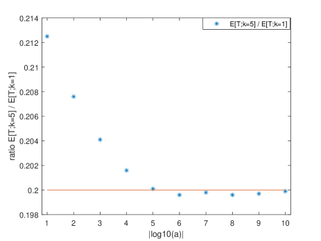
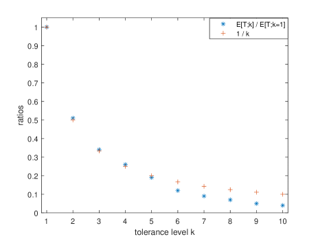
In order to verify the limit (103) as an approximation in the finite regime, we fix and select the thresholds of the sum-intersection rule in (63), via Monte Carlo simulation, so that the probability of at least errors, of any kind, is equal to . In Figure 2, we plot the ratio of the expected time for stopping for , over that for , against . In Figure 2, we can see that the expected time for stopping when reduces by a factor approximately equal to for , and clearly less than for . In Figure 2, we denote by the expected stopping time for the respective value of .
VII-B Controlling the generalized familywise errors
In the case of generalized familywise error rates, for and since , by Theorem V.2 as
| (104) |
where for , has the following form
| (105) |
and , , , , and are given in Table I.
| 1 | 2 | 3 | 4 | 5 | |
|---|---|---|---|---|---|
| 0 | 0 | 1 | 1 | 0 | |
| - | - | - | 0.61 | 0.61 | |
| - | - | - | - | 0.39 | |
| 0.69 | 0.69 | 0.66 | - | - | |
| 0.30 | 0.30 | 0.46 | 0.53 | - |
For the computation of we first use Algorithm 5, and then for the computation of , , , we used Algorithm 1. We can easily verify that is less than or equal to for all , and as a result
| (106) |
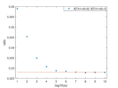
In Figure 3, we plot the ratio of the expected stopping time for over that for , against for . For each value of , and , the thresholds are selected according to (75). As expected by the form of in (105), it follows that this ratio converges to , which is also depicted in Figure 3, where by , we denote the expected stopping time for , , respectively.
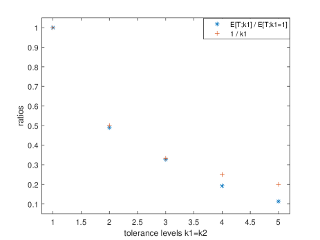
In order to verify the limit (106) as an approximation in the finite regime, we fix and we select the thresholds of the leap rule (73), via Monte Carlo sumulation, so that the probabilities of at least false positives and at least false negatives are both equal to . In Figure 4, we depict the ratio of the expected time for stopping with , over that for , against . In Figure 4, we observe that the expected stopping time for , reduces by a factor of approximately , as increases.
VIII Conclusion
In this work, we study the sequential anomaly identification problem in the presence of a sampling constraint under two different formulations that involve generalized error metrics. For each of them we establish a universal asymptotic lower bound, and we show that it is attained by a policy that combines the stopping and decision rule that was proposed in the case of full-sampling in [27] and a probabilistic sampling rule which is designed to achieve specific long-run sampling frequencies. The optimal performance is characterized, and the impact of the sampling constraint and tolerance to errors is assessed, both to a first-order asymptotic approximation as the error probabilities go to 0. These theoretical asymptotic results are also illustrated via simulation studies.
Directions for further research involve (i) the incorporation of prior information on the number of anomalous sources, as in [9] in the case of classical familywise error control , (ii) consideration of composite hypotheses for the testing problem in each source, as in [27] in the full sampling case, and in [12] for the case we know a priori that there is only one anomalous source and we can observe one source at a time, (iii) varying sampling or switching cost per source, as in [10] and [11], respectively. Other directions include the framework where the acquired observations are not conditionally independent of the past [19], as well as the consideration of a dependence structure within the observations from different sources [28].
Acknowledgments
This work was supported by the University of Illinois at Urbana–Champaign research support award RB21036.
References
- [1] A. Tsopelakos and G. Fellouris, “Sequential anomaly detection with observation control under a generalized error metric,” in 2020 IEEE International Symposium on Information Theory (ISIT), 2020, pp. 1165–1170.
- [2] R. J. Bolton and D. J. Hand, “Statistical Fraud Detection: A Review,” Statistical Science, vol. 17, no. 3, pp. 235 – 255, 2002. [Online]. Available: https://doi.org/10.1214/ss/1042727940
- [3] E. Dimson, Stock market anomalies. CUP Archive, 1988.
- [4] S. K. De and M. Baron, “Sequential bonferroni methods for multiple hypothesis testing with strong control of family-wise error rates i and ii,” Sequential Analysis, vol. 31, no. 2, pp. 238–262, 2012.
- [5] J. Bartroff and J. Song, “Sequential tests of multiple hypotheses controlling type i and ii familywise error rates,” Journal of statistical planning and inference, vol. 153, pp. 100–114, 2014.
- [6] Y. Song and G. Fellouris, “Asymptotically optimal, sequential, multiple testing procedures with prior information on the number of signals,” Electronic Journal of Statistics, vol. 11, 03 2016.
- [7] K. Cohen and Q. Zhao, “Active hypothesis testing for anomaly detection,” IEEE Transactions on Information Theory, vol. 61, no. 3, pp. 1432–1450, 2015.
- [8] B. Huang, K. Cohen, and Q. Zhao, “Active anomaly detection in heterogeneous processes,” IEEE Transactions on information theory, vol. 65, no. 4, pp. 2284–2301, 2018.
- [9] A. Tsopelakos and G. Fellouris, “Sequential anomaly detection under sampling constraints,” IEEE Transactions on Information Theory, pp. 1–1, 2022.
- [10] A. Gurevich, K. Cohen, and Q. Zhao, “Sequential anomaly detection under a nonlinear system cost,” IEEE Transactions on Signal Processing, vol. 67, no. 14, pp. 3689–3703, 2019.
- [11] T. Lambez and K. Cohen, “Anomaly search with multiple plays under delay and switching costs,” IEEE Transactions on Signal Processing, vol. 70, pp. 174–189, 2021.
- [12] B. Hemo, T. Gafni, K. Cohen, and Q. Zhao, “Searching for anomalies over composite hypotheses,” IEEE Transactions on Signal Processing, vol. 68, pp. 1181–1196, 2020.
- [13] A. Deshmukh, V. V. Veeravalli, and S. Bhashyam, “Sequential controlled sensing for composite multihypothesis testing,” Sequential Analysis, vol. 40, no. 2, pp. 259–289, 2021.
- [14] G. R. Prabhu, S. Bhashyam, A. Gopalan, and R. Sundaresan, “Sequential multi-hypothesis testing in multi-armed bandit problems: An approach for asymptotic optimality,” IEEE Transactions on Information Theory, 2022.
- [15] A. Tsopelakos and G. Fellouris, “Asymptotically optimal sequential anomaly identification with ordering sampling rules,” arXiv preprint arXiv:2309.14528, 2023.
- [16] H. Chernoff, “Sequential design of experiments,” Ann. Math. Statist., vol. 30, no. 3, pp. 755–770, 09 1959. [Online]. Available: http://dx.doi.org/10.1214/aoms/1177706205
- [17] S. Nitinawarat, G. K. Atia, and V. V. Veeravalli, “Controlled sensing for multihypothesis testing,” IEEE Transactions on Automatic Control, vol. 58, no. 10, pp. 2451–2464, 2013.
- [18] S. A. Bessler, “Theory and applications of the sequential design of experiments, k-actions and infinitely many experiments, part i theory.” Department of Statistics, Stanford University, Technical Report 55, 1960.
- [19] S. Nitinawarat and V. V. Veeravalli, “Controlled sensing for sequential multihypothesis testing with controlled markovian observations and non-uniform control cost,” Sequential Analysis, vol. 34, no. 1, pp. 1–24, 2015. [Online]. Available: https://doi.org/10.1080/07474946.2014.961864
- [20] J. Bartroff, “Multiple hypothesis tests controlling generalized error rates for sequential data,” Statistica Sinica, vol. 28, no. 1, pp. 363–398, 2018. [Online]. Available: http://www.jstor.org/stable/26384246
- [21] J. Bartroff and J. Song, “Sequential tests of multiple hypotheses controlling false discovery and nondiscovery rates,” Sequential Analysis, vol. 39, no. 1, pp. 65–91, 2020. [Online]. Available: https://doi.org/10.1080/07474946.2020.1726686
- [22] X. He and J. Bartroff, “Asymptotically optimal sequential fdr and pfdr control with (or without) prior information on the number of signals,” Journal of Statistical Planning and Inference, vol. 210, pp. 87–99, 2021. [Online]. Available: https://www.sciencedirect.com/science/article/pii/S0378375820300604
- [23] Y. Benjamini and Y. Hochberg, “Controlling the false discovery rate: a practical and powerful approach to multiple testing,” Journal of the Royal statistical society: series B (Methodological), vol. 57, no. 1, pp. 289–300, 1995.
- [24] E. L. Lehmann and J. P. Romano, “Generalizations of the familywise error rate,” The Annals of Statistics, vol. 33, no. 3, pp. 1138–1154, 2005. [Online]. Available: http://www.jstor.org/stable/3448684
- [25] J. P. Romano and A. M. Shaikh, “Stepup procedures for control of generalizations of the familywise error rate,” The Annals of Statistics, vol. 34, no. 4, pp. 1850–1873, 2006. [Online]. Available: http://www.jstor.org/stable/25463487
- [26] J. P. Romano and M. Wolf, “Control of generalized error rates in multiple testing,” The Annals of Statistics, vol. 35, no. 4, pp. 1378–1408, 2007. [Online]. Available: http://www.jstor.org/stable/25464544
- [27] Y. Song and G. Fellouris, “Sequential multiple testing with generalized error control: An asymptotic optimality theory,” The Annals of Statistics, vol. 47, no. 3, pp. 1776 – 1803, 2019. [Online]. Available: https://doi.org/10.1214/18-AOS1737
- [28] J. Heydari, A. Tajer, and H. V. Poor, “Quickest linear search over correlated sequences,” IEEE Transactions on Information Theory, vol. 62, no. 10, pp. 5786–5808, 2016.
- [29] P. Hall and C. C. Heyde, “Martingale limit theory and its application,” Probability and Mathematical Statistics. New York etc.: Academic Press, A Subsidiary of Harcourt Brace Jovanovich, Publishers. XII, 308 p. $ 36.00 (1980)., 1980.
- [30] O. Kallenberg, Foundations of Modern Probability, ser. Probability and Its Applications. Springer New York, 2002. [Online]. Available: https://books.google.com/books?id=TBgFslMy8V4C
- [31] E. Cesàro, “Sur la convergence des séries,” Nouvelles annales de mathématiques: journal des candidats aux écoles polytechnique et normale, vol. 7, pp. 49–59, 1888.
Appendix A
In Appendix A, we prove Lemma III.1 and Lemma III.2, which provide the solutions to the max-min problems (18) and (30), respectively. We also provide Algorithm 1 for the computation of and , and Algorithm 5 for the computation of .
Proof:
Since is compact, and is finite, the max-min problem (18) has a solution. The max-min structure of (18) implies that a maximizer must satisfy the following two conditions:
-
(i)
for each , and each , it holds
(107) -
(ii)
the follow an ascending order, i.e.,
(108)
By definition of in (16), the first condition (107) implies that
| (109) |
To prove why condition (107) must hold, we apply an argument by contradiction. Let us assume that there are , and such that , and let us denote by the index which corresponds to smallest such , in case the assumed inequality holds for more than one , and by the index which corresponds to largest such in case the assumed inequality holds for more than one . Clearly, , and the is included in the sum of , as it is one of the smallest , whereas is not included. Since , and by definition , then . Thus, simply by swapping the values of , we could increase the value of by a size of , which is a contradiction because is a maximizer.
Assuming that (107) holds which implies (109), in order to prove why condition (108) must hold, we apply again an argument by contradiction. Let us assume that there are , both in , such that . In such a case, it is clear that because by definition . If we swap the values of , , then we can increase the value of since
| (110) |
which is a contradiction because is a maximizer.
The maximizer with the minimum norm is the one that satisfies (108), and (107) by the following equality,
| (111) |
If is large enough so that
| (112) |
then the maximizer with the minimum norm is
| (113) | ||||
which implies that
and thus equals to the form (19) with , , . Hence, it suffices to prove that equals to the form (19) when
| (114) |
When (114) holds, the maximizer satisfies
| (115) |
by which we get that
where the second equality follows by (111). Therefore,
| (116) |
where defined in (15) is the harmonic mean of the largest elements in , and it stands for an average of them. It holds
| (117) |
because
since for all . By replacing in (109) we get
| (118) |
Therefore, the values of are deduced by the solution of the following maximization problem
| (119) |
with respect to and subject to
-
(i)
-
(ii)
-
(iii)
In the special case , and since by definition , the maximization method is to distribute so that respectively takes its’ largest possible value, independently, one by one with respect to the priority list they are written. On the other hand, if then would become first in the priority list. Due to constraint (iii) for any value of , the value of must be large enough so that the inequality is satisfied. Thus, the maximization method for the former case does not work, as the value of depends on the value of . In order to resolve this issue, we consider
thus reduces to
| (120) |
and it holds
The values of are deduced by the solution of the following maximization problem,
| (121) |
with respect to and subject to
-
(i)
-
(ii)
-
(iii)
If
| (122) |
then ,
| (123) |
and thus equals to the form (19) with , , , . Therefore, in view of (114), it suffices to prove that equals to the form (19) when
| (124) |
If satisfies (124) then , the objective of (121) becomes
and if we set , the maximization problem (121) takes the more general form
| (125) |
with respect to and subject to
-
(i)
-
(ii)
-
(iii)
For any with , if
| (126) |
then our priority is to make as large as possible. If then we decrease variable by . We observe that the value of does not affect as the values interfere. If (126) does not hold, our priority is to make as large as possible. If then we set equal to , and we increase by . Depending on the size of this procedure continues for a number of times, and it ends up with a form
| (127) |
In order to prove that the maximizer with the minimum norm satisfies (21)-(25), we observe that (23)-(25) follow directly by the form (127) of by matching the with the factor of the respective . In order to prove (21) we distinguish the following two cases.
-
(i)
If then and the result follows by (111).
-
(ii)
If then
which proves the claim since .
∎
In Algorithm 1, we describe explicitly how are computed. The algorithm primarily focuses on the case that satisfies (124), as the other two cases are covered in (112) and (122). Algorithm 1 solves the constrained optimization problem (125) by implementing the steps described in the paragraph that follows (126).
-
(1)
Input: , , .
-
(2)
Compute
-
(3)
If then
, , , ,
go to output
end-if.
-
(4)
If then
, , , ,
go to output
end-if.
-
(5)
Initialize: , , ,
,
.
-
(6)
While
-
(i)
If or then
-
If then
,
,
-
else
,
,
end-if
end-if
-
-
(ii)
If or then
,
,
.
-
If then
,
,
end-if
end-if
-
end-while.
.
-
(i)
-
(7)
Output: , , , .
Proof:
For the proof of Lemma III.2, it suffices to show that
where is the maximizer with the minimum norm of the problem (32), then the form (34) of , as well as the form (36)-(45) of the maximizer of (30) with the minimum norm, follow by Lemma III.1.
Since is compact and , are finite sets, the max-min problem (30) has a solution. We denote by the maximizer of (30) with the minimum norm, where , , and we consider
| (128) |
The max-min structure of (30) implies that for , , we have
and
Hence,
| (129) |
and since we have .
Therefore, it suffices to prove that is the maximizer of (32) with the minimum norm. To prove this, we apply an argument by contradiction. Let us assume that is not a maximizer of (32), then there is such that , and
Let us denote by the maximizer of , and by the maximizer of . Then,
which is a contradiction because we assumed that is a maximizer of (30). Also, if we assume that is not the maximizer (32) with the minimum norm, by (128) we deduce that is not the maximizer of (30) with the minimum norm, which is a contradiction. ∎
Next, we provide Algorithm 5 for the computation of the maximizer of the constrained optimization problem (32) with the minimum norm.
-
1(1)
Input: , , , , , .
Compute
If
root of the equation with respect to .
.
root of the equation with respect to .
end-if
If
root of the equation with respect to .
.
root of the equation with respect to .
end-if
Output: .
We note that (resp. ) and (resp. ) are unique can be computed using the bisection method. Without loss of generality, we assume that
then for the computation of , we consider the function
which is continuous with
If then , otherwise and the solution follows by the bisection method. Since is increasing over , the function is also increasing over and thus is unique.
For the computation of , we consider the function
| (130) |
which is continuous with
Thus, the solution follows by the bisection method and it is less than or equal to . Since is increasing over , and is non-increasing over the function is increasing over and thus is unique.
By restricting the value of to , we do not reduce the maximum possible value that the objective of (32), i.e. , can take. In the same time, we restrict the number of possible maximizers to , by keeping the one with the minimum norm, which is given by the unique root of
Appendix B
In Appendix B, we prove Theorems IV.1, IV.2, IV.3, which establish a universal asymptotic lower bound on the expected stopping time when controlling the misclassification error rate (7), and the familywise error rates (9), respectively.
B-A Misclassification error rate
As a first step towards the proof of Theorem IV.1 we provide the following auxiliary lemma. We fix , and we denote by the family of subsets of whose Hamming distance from is at least , i.e.,
| (131) |
Lemma B.1
For any , and , we have the following inequality,
| (132) |
Proof:
We fix , and we denote by the set minimizer of
| (133) |
where in place of we have . By [27, Lemma B.2], there exists a set such that for the sets it holds
| (134) |
By the right inclusion we have
| (135) |
which means that , whereas by the left inclusion we have
| (136) |
As a result,
| (137) | ||||
where the first inequality follows by the fact that , and the second one by (136). The set minimizer has Hamming distance equal to , for any , as the addition of extra terms exceeds the minimum, which implies
| (138) | ||||
where the last equality follows by definition of according to (18). ∎
For the proof of Theorem IV.1, we introduce the log-likelihood ratio of versus , for any sampling rule and any subsets , based on the observations from all sources in the first sampling instants, i.e.,
| (139) |
Since is -measurable, is independent of , and is independent of and of , we have
| (140) | ||||
where we recall that , and we set . Comparing with (62), it is clear that
| (141) |
We also set
| (142) | ||||
which implies that
| (143) |
Proof:
We have to show that
| (144) |
where is a quantity that tends to zero as . We set
| (145) |
By Markov’s inequality, for any stopping time and we have
| (146) |
Thus, it suffices to show that for every we have
| (147) |
as this will imply that
| (148) |
and the desired result will follow by letting .
In the rest of the proof we fix some arbitrary . Then, for any , , and , where is defined in (131), we have
| (149) | ||||
where is an arbitrary constant in . By summing up (149) with respect to all , we have
| (150) | ||||
In view of the fact that
| (151) |
we obtain
| (152) | ||||
Thus, in order to show (147), it suffices to show that for any
| (153) |
and
| (154) |
In order to show (153), we fix and . By application of Boole’s inequality we have
| (155) |
For all , we apply the change of measure and by Wald’s likelihood ratio identity we obtain
| (156) | ||||
where the last inequality is deduced by the fact that for any , it holds . In view of (155), we obtain
| (157) |
Since is arbitrary, letting , we prove (153).
B-B Familywise error rates
As a first step towards the proof of Theorems IV.2, IV.3, we provide the following auxiliary lemma. To this end, for fixed , we consider the set
| (164) |
and for any , we also consider the sets
| (165) | ||||
Lemma B.2
For any and , we have the following inequalities:
-
(i)
If ,
(166) -
(ii)
If ,
(167) - (iii)
Proof:
We prove (i), (iii). Case (ii) is symmetric to (i).
For , without loss of generality, we consider such that , or equivalently and , otherwise (166) holds trivially. Since , there exists such that , and contains the sources that correspond to the smallest terms in . Clearly, , and
| (169) |
Since , even if contains the smallest elements in , the set contains the following smallest elements in . Thus, let us denote by the identity of the source with the smallest element in , then we have
| (170) | ||||
For , without loss of generality, we consider such that and , or equivalently and , otherwise (168) holds trivially. We consider the quantities
| (171) |
-
1.
The fact that implies that . Thus, there exists such that , and contains the sources that correspond to the smallest elements in . We set . Since , it holds , and
(172) Therefore,
which implies , and
(173) Even if contained the smallest elements in , the set would contain the following smallest elements in the same set. Thus, for to denote the identity of the smallest element in , we always have
(174) -
2.
The fact that implies that . Thus, there exists such that and contains the sources that correspond to the smallest elements in . We set . Since , it holds , and
(175) Therefore,
which implies , and
(176) Even if contained the smallest elements in , the set would contain the following smallest elements in the same set. Thus, for to denote the identity of the source with the smallest element in , we always have
(177)
We proceed to the proof of Theorem IV.3 and by which we deduce the proof of Theorem IV.2, as explained in the last part of the following proof.
Proof:
We have to show that
| (179) |
where is defined in Theorem IV.3 and is a quantity that tends to zero as . We define
| (180) |
By Markov’s inequality, for any stopping time and ,
| (181) |
Thus, it suffices to show that for every , we have
| (182) |
as this will imply that
| (183) |
and the desired result will follow by letting .
In the rest of the proof, we fix some arbitrary . Moreover, we note that for any we have either or , because otherwise , which contradicts the assumption . In what follows, we let and we focus on the case and . The other two cases , and are simpler and they can be treated in the same way as described in the last part of this proof.
Then, for any and we have
| (184) | ||||
where is defined in (140), and is an arbitrary constant in . The third term in (184) can be equivalently written as
| (185) |
where .
For simplicity in what follows we just write instead of . We upper bound the third term in (184) by
| (186) | ||||
By summing up (184) over all , we have
In view of the fact that
| (187) |
we obtain
Thus, in order to show (182) it suffices to show that for all
| (188) | |||
and
| (189) | ||||
where the supremum is evaluated over . In order to show (188), we apply Boole’s inequality and we have:
| (190) | ||||
For all , we apply the change measure , and we have
| (191) | ||||
where the last inequality is deduced by the fact that for any , the error constraint (9) implies . Therefore, for every ,
| (192) |
In the same way, we show that
| (193) |
Letting , we prove (188).
In order to show (189), we observe that by decomposition (143) we have
| (194) | |||||
which further implies that
| (195) | ||||
We note that for any fixed ,
| (196) |
where is defined in (50). Also, by Lemma B.2 we have
| (197) |
Therefore,
| (198) |
As a result, the probability in (189) is bounded above by
| (199) |
where
| (200) |
and it suffices to show that
| (201) |
In order to show (201), it suffices to prove that
| (202) |
and then the claim follows by [27, Lemma F.1]. Indeed, by [29, Theorem 2.19] and moment assumption (12) we have
| (203) |
The other cases: As for the cases , and we note the following.
-
•
In case , , i.e., and for any , we have
(204) This also applies for the case .
-
•
In case , , i.e., and for any , we have
(205) This also applies for the case .
In both cases, we deduce the claim following the same reasoning as for the main case (). ∎
Appendix C
In Appendix C, we prove Theorems V.1, V.2, Theorems VI.1, VI.2, and Proposition VI.1. Throughout Appendix C, we fix .
Proof:
In view of the asymptotic lower bound in Theorem IV.1, it suffices to show that
| (206) |
where is the stopping rule defined in (63). For selected according to (65), it suffices to show that for an arbitrarily small , we have
| (207) |
where are defined in (66), and by letting we obtain (206). To this end, we fix small enough, and we set
| (208) |
for which it holds
| (209) |
On the event , there exists with such that
| (210) |
Moreover, for every we have
By Lemma III.1, for every set with , we have
which further implies that there is an sufficiently smaller than such that
Therefore, for every the event is included in the event
In view of (209) and by application of Boole’s inequality over all such that , we deduce that
| (211) |
where
| (212) | ||||
By assumption, for any , , and for any , we have
| (213) | |||
and thus by [9, Lemma A.2 (i), (ii)], with and , it follows that all the series in (211) converge. Hence, letting we obtain (207). ∎
Proof:
In view of the asymptotic lower bound in Theorem IV.3, it suffices to show that
| (214) |
where is the stopping rule (73). Without loss of generality, we focus on case and equals (53) of Theorem IV.3, as the other cases follow by the same approach. For selected according to (75) it suffices to show that for any arbitrarily small , we have
| (215) |
where , are defined as in (80)-(81), and by letting we obtain (214). To this end, we fix small enough and we set
| (216) |
and we observe that
| (217) |
For any , on the event there exist with , and with , such that
| (218) |
Moreover, for every we have
| (219) |
For any set , , as described above, we have
Thus, there is an sufficiently smaller than such that
| (220) |
Therefore, for every the event is included in the event
In view of (217) and by application of Boole’s inequality over all with , and all with , we deduce that
| (221) | ||||
In order to prove the claim, it suffices to show the summability of the series in (221). By Boole’s inequality we have
| (222) | ||||
By assumption, for any , , and for any we have
| (223) | ||||
and thus by [9, Lemma A.2 (i) (ii)], with and , it follows that all the series in (222) converge. Thus, letting we obtain (215).
∎
Proof:
By definition of , we have
| (224) | ||||
which by Boole’s inequality is further bounded by
| (225) | ||||
Therefore, in order to prove that , it suffices to show that
| (226) | ||||
We prove the case , as the case follows in the same way. We note that
| (227) | ||||
In view of assumption (91), in order to prove (226), it suffices to show that
| (228) |
and since
| (229) | ||||
it suffices to show
| (230) |
By Markov’s inequality
| (231) |
For each , is a -martingale, thus by Rosenthal’s inequality [29, Theorem 2.12] there is a constant , such that
| (232) |
and as a result,
| (233) |
For small enough such that , it holds
| (234) |
which proves the claim (230). ∎
Proof:
According to Theorems V.1 and V.2, it suffices to show that for each
| (235) |
where is defined according to Definitions V.1 and V.2, respectively.
By the definition (92) of a probabilistic sampling rule, is conditionally independent of given . Thus, by [30, Prop. 6.13] there is a measurable function such that
| (236) |
where is a sequence of iid random variables, uniformly distributed on . Consequently, for each there is a measurable function such that
| (237) |
We fix , and . For every , we have
| (238) | ||||
and as a result
| (239) | ||||
For the first term on the right hand side of (239) we have
| (240) | ||||
where we used the fact that for all . Since is consistent both terms on the right hand side of (240) are summable.
For the second term on the right hand side of (239) we have
| (241) | ||||
By the (general form of) Stolz-Cesaro theorem [31],
| (242) | ||||
where the last inequality is deduced by assumption (95). Therefore, there exists an such that for all it holds
| (243) |
Hence,
| (244) | ||||
and, thus, it suffices to show that
| (245) |
| (246) |
which shows that is a martingale difference sequence, whose absolute value is uniformly bounded by . By application of Azuma-Hoeffding inequality, we deduce that
| (247) |
where is a constant, which proves (245).
∎
Proof:
We show that the suggested sampling rule is consistent for part (ii). According to Theorem VI.1, it suffices to show that for each ,
| (248) |
for some and . We choose . We fix , and for every , we notice that
| (249) | ||||
By (99), we have , for all , and we deduce that
| (250) |
which further implies
| (251) | ||||
In view of (93), it holds
| (252) |
which shows that is a martingale difference, whose absolute value is also uniformly bounded by . Thus, by application of the Azuma-Hoeffding inequality, we deduce that
where is a constant. Therefore, we deduce (248) by noting that there is such that for all ,
∎