A simple model for longitudinal electron transport during and after laser excitation: Emergence of electron resistive transport
Abstract
Laser-driven electron transport across a sample has garnered enormous attentions over several decades, as it provides a much faster way to control electron dynamics. Light is an electromagnetic wave, so how and why an electron can acquire a longitudinal velocity remains unanswered. Here we show that it is the magnetic field that steers the electron to the light propagation direction. But, quantitatively, our free-electron model is still unable to reproduce the experimental velocities. Going beyond the free electron mode and assuming the system absorbs all the photon energy, the theoretical velocity matches the experimental observation. We introduce a concept of the resistive transport, where electrons deaccelerate under a constant resistance after laser excitation. This theory finally explains why the experimental distance-versus-time forms a down-concave curve, and unifies ballistic and superdiffusive transports into a single resistive transport. We expect that our finding will motivate further investigations.
I Introduction
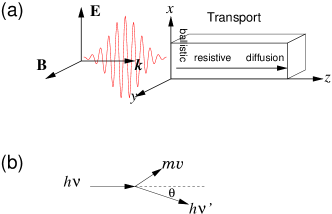
Electron transport is a common phenomenon that occurs in various forms. An electron can diffuse under a temperature or concentration gradient, often described by the diffusion equation schafer , where is the electron density, is the diffusion constant and is the relaxation time. If an electric field is applied, one can describe it through the Boltzmann equation mahan2000 ; riffe2023 , , where is the electron distribution function, is the electron velocity, is its position, is the electron mass, and is the electric field. When one applies a voltage bias along the axis across a device, the electron inside the device moves along the axis. This is how classical physics explains electron transport. When the device becomes shorter, one has a ballistic transport, where the electron travels like a bullet without resistance inside the device datta . Now, consider a linearly-polarized laser pulse, propagating along the axis and with its electric field along the axis and the magnetic field along the axis, is applied on to the same device (Fig. 1). It is obvious that the electron will move along the axis, since is along the . But there is no electric field along the axis. So does the electron travel along the longitudinal direction?
The answer is affirmative. In 1987, Brorson et al. brorson1987 employed a 96-fs laser pump pulse of wavelength 630 nm and of fluence 1 mJ/cm2 to excite a group of thin gold films of thickness from 200 to 3000 from the front, and then detected the reflected probe beam from the back of the sample. They found that the electron can travel at 108 cm/s, very close to the Fermi velocity of electrons in Au. In 2011, Melnikov et al. melnikov2011 employed the same experimental setup, but with a magnetic film Au/Fe/MgO(001), where the thickness of Fe is 15 nm and that of Au is 50 and 100 nm. They sent in a -polarized 35-fs pump pulse of 800 nm on to the Fe layer through the MgO substrate, and then detected the magnetic second-harmonic (MSH) signal reflected from the back of the Au layer. They found the MSH hysteresis loop after 30 fs delay between the pump and probe, even with fluence 1 mJ/cm2 and energy 40 nJ per pulse. These results attracted a broad interest choi2014 ; vodungbo2012 ; pfau2012 ; kimling2017 ; hofherr2017 ; seifert2017 ; seifert2018 ; chen2019 . Besides MSH, Beyazit et al. beyazit2020 ; beyazit2023 employed the time-resolved two-photon photoemission and found that the electron lifetimes are shorter when the thickness of their Au layer increases. They concluded the excited electrons propagate through Au in a superdiffusive regime battiato2012 , but ballistically across the interfaces. The transition from a superdiffusive to a diffusive transport occurs around 20-30 nm of the Au layer kuhne2022 . Using the same technique, Bühlmann et al. buhlmann2020 detected 4% spin polarization change in the Au film, consistent with that of Hofherr et al. hofherr2017 . Recently, Karna et al. karna2023 reported that the ballistic length of hot electrons in gold films exceeds 150 nm, 50% larger than 100 nm from prior studies. But their experimental geometry is different. They measured the lateral motion (along the traverse direction), not along the longitudinal direction brorson1987 ; hohlfeld2000 .
Theoretically, several models are proposed. Salvatella et al. salvatella2016 proposed the analytical model of the demagnetization amplitude, where they linked the absorbed energy to the temperature change and then to the demagnetization. Another one is the superdiffusion model battiato2012 , where one assumes a time-dependent diffusion exponent and then solves the diffusion equation for the electron. These theories build in a gradient from the beginning, but how such a gradient is established is not addressed. This boils down to the fundamental question: why and how the electron could gain the longitudinal velocity liu2023 ; kang2023 ; malinowski2018 . In atoms and plasma physics, a similar problem has been studied before yang2011 ; maurer2021 , but with the laser fluence over J/cm2, which has little relevance to laser-induced electron transport in a real device.
Given the complexity of the problem jang2020 , we have two moderate objectives. First, we limit ourselves to a simpler question: Is it possible to understand laser-induced electron transport qualitatively using a free-electron model? We employ Varga and Török’s method, which is based on the Hertz vector. We carry out a series of simulations by solving the Newtonian equation of motion of the electron. We find that the longitudinal velocity is a joint effect of the electric and magnetic fields of the laser pulse. However, using the same experimental laser parameters razdolski2017 , we are still unable to quantitatively reproduce the experimental results. Going beyond the free electron model and assuming all the photon energy absorbed into the system, we find that the electron velocity then matches the experimental ones. Second, after laser excitation, we introduce a new concept of the resistive transport, where hot electrons deaccelerate under a constant resistance from other electrons and ions. This does not only explain why experimentally heckschen2023 ; suarez1995 the dependence of the electron time on the electron distance is a down concave, but also unifies the ballistic transport xiong2017 ; suslova2018 and the superdiffusive transport battiato2012 as a single resistive transport. Our finding will have an important impact on the future investigation of ultrafast electron and spin transport brorson1987 ; melnikov2011 ; stanciu2007 ; mplb18 ; aip20 .
The rest of the paper is arranged as follows. Section II is devoted to our theoretical formalism. Numerical results during the laser excitation are given in Sec. III, where we compare our results with the Compton scattering and the experimental results. In Sec. IV, we compare and contrast four models with the latest experimental data. Section V introduces the resistive transport theory after the initial excitation. We conclude this paper in Sec. VI.
II Formalism
We consider a free electron placed inside a laser field, with its electric-field E along the axis and the magnetic field B along the axis. Figure 1(a) schematically illustrates a typical experimental geometry, where the laser pulse propagates toward the sample along the axis. The Hamiltonian of the electron inside an electromagnetic field is
| (1) |
where is the vector potential, is the scalar potential, and are the electron mass and charge, respectively. The equation of motion is given in terms of the generalized Lorentz force as griffiths2018 ,
| (2) |
If we set to zero, then every term, except the first term, on the right side, is zero, so the electron only moves along . This demonstrates that it is indispensable to include .
We follow Varga and Török varga1998 , and start from the Hertz vector, which satisfies the vectorial Helmholtz equation, so the resultant electric and magnetic fields automatically satisfy the Maxwell equation, given in an integral form. Within the paraxial approximation, we get the reduced and ,
| (3) |
The final electric and magnetic fields are
| (4) |
where is the field amplitude and is the pulse spatial width chosen as . is the wavelength of the pulse. When the light enters a sample, both fields are reduced by , where is the penetration depth and 2 comes from the fact that penetration depth is defined at the incident fluence and the fluence is proportional to the square of the electric field. is chosen to be 14 nm, typically values in fcc Ni.
In our study, we choose a linearly -polarized pulse that is propagating along the axis. The pulse is a Gaussian of duration , amplitude and photon energy . in and in Eq. 4 is replaced by , so our electric and magnetic fields are
| (5) | |||||
| (6) |
These analytic forms of and , which contain both the spatial and temporal dependences, greatly ease our calculation. As a first step toward a complete transport theory, we treat the electron classically, and solve the Newtonian equation of motion numerically,
| (7) |
where is the electron velocity. Although our method is classical, it fully embraces the real space approach that is more suitable for transport, a key feature that is often missing from prior first-principles and model simulations. This will answer the most critical question why the electron can move along the axial direction.
III During laser excitation
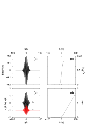
We start with the experimental laser parameters from Razdolski et al. razdolski2017 , where their laser fluence is mJ/cm2, duration fs, and photon energy of eV. These parameters are typically used in experiments jpcm10 . We use ourbook to find the electric field amplitude to be . Our electric field is shown in Fig. 2(a). The initial position and velocity of the electron are set to zero. Figure 2(b) shows the velocity and position oscillate strongly with time. The maximum velocity reaches , , on the same order of magnitude of the velocity in ch1 Co/Pt multilayers bergeard2016 and also that of the experiment in Co/Cu(001) films wieczorek2015 . Because the kinetic energy is proportional to the velocity, the electron must heat up. If we include the band structure of a solid, it will stimulate both intraband and interband transitions jpcm23 , leading to demagnetization and magnon generation jap19 . We see that the final is close to zero, so the electron heating is local, the local heating. For clarity, in Fig. 2(b) we shift by one unit down.
The velocity along the axis, , is very different. Figure 2(c) shows is always positive, and increases with time, without oscillation. It reaches /fs. The positivity of , regardless of the type of charge, is crucial to the electron transport, and can be understood from the directions of and B. Suppose at one instant of time, E is along the axis and B along the axis. The electron experiences a negative force along the axis and gains the velocity along the axis, so the Lorentz force due to B is along the direction. Now suppose at another instance, E changes to and B to , so the electron velocity is along , but the Lorentz force is still along the axis. If we have a positive charge, the situation is the same. The fundamental reason why we always have a positive force is because the light propagates along the axis and the Poynting vector is always along and points along the axis. We test it with various laser parameters and do not find a negative , in agreement with Gao gao2004 . Under cw approximation, Rothman and Boughn rothman2009a gave a simple but approximate expression for the dimensionless , and Hagenbuch hagenbuch1977 gave , both of which are positive. Therefore, both their theories and our numerical results agree that the axial motion of the electron is delivered by both E and B. This is also consistent with the radiation pressure from a laser beam can accelerate and trap particles ashkin1970 ; ashkin1986 . Figure 2(d) shows that reaches 1.66 at 100 fs. Naturally, the electron can move further as time goes by until it collides with other electrons and ions.
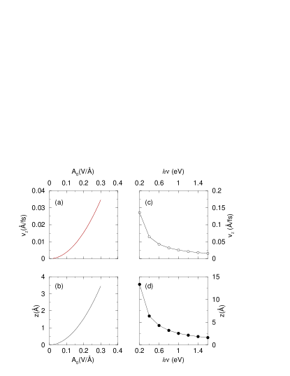
Keeping the rest of laser parameters unchanged, i.e., eV and fs, we increase the laser field amplitude from 0.02 to 0.30 . Figure 3(a) shows the final velocity as a function of . We notice that change is highly nonlinear. We fit it to a quadratic function, , where is a constant of 0.383898 /(fsV/)2, and find that the fit is almost perfect. Because is directly proportional to the fluence, this demonstrates is linearly proportional to the laser fluence, which is exactly expected from the Poynting vector . Thus, both qualitatively and quantitatively our results can be understood. Since the displacement follows the velocity, it also increases with quadratically (see Fig. 3(b)).
With growing interest in THz pulses, we investigate the photon energy dependence of and . We increase from 0.2 up to 1.6 eV, while keeping both the duration fs and amplitude fixed. Figure 3(c) shows an astonishing result: both and are inversely proportional to . At the lower end of , reaches 0.136 /fs and reaches 13.34 (see Fig. 3(d)). Note that at such a low amplitude, a pulse of 1.6 eV only drives the electron by 1.60 . This explains why THz pulses become a new frontier for ultrafast demagnetization shalaby2015 ; hudl2019 ; lee2021 . Polley et al. polley2018 employed a THz pulse to demagnetize CoPt films with a goal toward ultrafast ballistic switching. Shalaby et al. shalaby2018 showed that extreme THz fields with fluence above 100 mJ/cm2 can induce a significant magnetization dynamics in Co, where the magnetic field becomes more important. ch4 Very recently, using multicycle 2.5-THz pulses, Riepp et al. riepp2024 reported incoherent and coherent magnetization dynamics in labyrinth-type Co/Pt multilayers. ch4end Our result uncovers an important picture. When the pulse oscillates more slowly, the electron gains more grounds. Of course, a DC current can move electrons even further, but then it does not have enough field intensity. This result can be tested experimentally.
III.1 Comparison with prior theories
To the best of our knowledge, there has been no investigation using the experimental laser parameters razdolski2017 as we did, so we decide to compare our results with that of Compton scattering. This comparison is possible because we use a free-electron model.
Assume that the initial kinetic energy of the electron is zero. The kinetic energy gained from the photon must be equal to the loss in the photon energy as
| (8) |
where is the electron velocity, is the number of photons that interact with the electron and is the frequency change computed from the wavelength change as . The wavelength change is , where is the outgoing angle of the photon with respect to the incident direction (see Fig. 1(b)). We directly compute the velocity of the electron as
| (9) |
If we use Brorson’s experimental wavelength, we find m/s. Except that we have an enormously large , the electron velocity is around 103 m/s. Figure 2(c) shows the final velocity is /fs or 1.65 m/s. Therefore, both approaches agree with each other very well.
III.2 Comparison with experiments
Although Razdolski et al. razdolski2017 estimated the axial displacement on the order of 2 nm, it is harder to compare because it depends on the relaxation time of the electron in a particular material. Instead, majority of experiments measured the velocity. Brorson brorson1987 gave m/s for Au. Melnikov melnikov2011 found that a delay of 40 fs for a 50 nm of Au, so the velocity is m/s.
These velocities are three orders of magnitude larger than our theoretical value above. This shows that although our model does yield the correct direction of the electron motion, the free electron model, which is sufficient for atomic and plasma physics, is not adequate for metals, at least for the transport property induced by laser. In the following, we discuss several possible solutions for future research.
IV Beyond the free-electron model
Given the above finding, it is very appropriate to discuss a few alternative theories, as they are crucial to experiments malinowski2018 .
IV.1 Drude model
We recall first that in metals, the Drude model is often used for the electric transport, where a voltage bias is applied along the longitudinal direction. If an electric field (constant) is along the direction, the electron momentum change is given as , which will grow with time infinitely. Drude realized that the electron must experience collisions from other electrons and ions, so the electron will lose its momentum, whose value is given by . At equilibrium, these two must be equal, so the drift velocity is , where is the relaxation time, not to be confused with the above laser pulse duration. in metals is around 0.1 m/s ohanian .
In laser excitation, there is no such field. It is possible to include the magnetic field into the Drude model, but as seen above, this will lead to the same conclusion as our free electron model.
IV.2 Diffusion transport
Diffusion transport has been proposed to understand the electron transport. However, there is a shortcoming in these theories. They do not specify how these initial gradients are established. For instance, Choi et al. choi2014 ; choi2014b and Fognini et al. fognini2017 replaced the particle density by the chemical potential as where is the spin chemical potential and is the spin diffusion constant, and is the spin relaxation time. How a nonzero appears is not given. This is also true for the superdiffusion model battiato2012 , where the initial velocity of the electron is considered as an input parameter and is not possible to compare with the experimental velocity.
IV.3 Boltzmann equation
The third possibility is to use the Boltzmann equation. The distribution function, , under the influence of the laser field, changes as thomas1966 ; kittel ; mahan1987
| (10) |
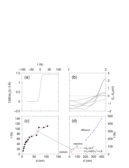
where . We are only interested in because this is along the axial direction, . Since we already know and , we can compute it easily. Figure 4(a) shows how changes with time. We see that is very small, whose largest value is around . However, it is sufficient to move electrons in solids. We take fcc Ni as an example. Figure 4(b) shows the band structure of fcc Ni along the -Z direction. There are five bands across the Fermi energy. Regardless of how small is, the laser field is able to lift electrons from an occupied band to an unoccupied band, i.e., the intraband transition jpcm23 . Now the questions is whether we have enough photons.
We can estimate the number of photons on the surface of a unit cell from the experiments. We take bcc Fe as an example. Its lattice constant is , so its cross section is . The experimental fluence melnikov2011 is mJ/cm2 and the photon energy is eV, so the number of photons per unit cell is . One bcc cell has two Fe atoms, so each Fe atom receives photons. If we assume that these photons are absorbed, , we find m/s. For fcc Au, using Brorson’s experimental data, we find the number of photons per unit cell to be 5.2746. Each Au atom receives 1.32 photons. We find m/s, which agrees with the experimental value of 108 cm/s almost perfectly. Therefore, we believe that it is very likely that a quantum theory, which includes the magnetic field and the band structure, will be able to explain experimental results quantitatively.
V After initial excitation: Resistive transport theory
Once electrons have enough velocity, they will travel through the materials brorson1987 . There are three different theories for transport. Ballistic and diffusive transports are two traditional ones knorren2002 ; chan2009 . But their separation has not been very clear. In 1998, Bron et al. bron1998 concluded that “the transport of quasi-electrons arriving at the peaks is neither purely ballistic nor purely diffusive”. This unclear region is termed the superdiffusive transport battiato2012 , but its physics remains unclear. The reason is that for a long time, there have been very few thickness dependence experiments, besides those earlier ones brorson1987 ; juhasz1993 ; suarez1995 ; melnikov2011 . Heckschen et al. heckschen2023 carried out a systematic time-resolved two-photon photoemission (2PPE) measurement as a function of the thickness of Au films from 5 to 105 nm in the Au/Fe/MgO structure. The thickness of Fe is fixed at 7 nm. 2PPE employs two laser pulses. The pump pulse hits on the back of the iron film through the MgO substrate and pushes electrons toward the interface between Fe and Au layers. These hot electrons pass through the interface and enter the Au layer. Once they reach the surface of Au, a probe pulse of 4 eV knocks them out. Experimentally, Heckschen et al. collected the electrons as a function of kinetic energy after each time delay between the pump and probe. At eV, where is the electron energy and is the Fermi energy, they obtained an accurate dependence of the reduced time delay (see their paper for detail) as a function of . We use Webdigitizer web to read off their experimental data from their Fig. 4 and reproduce them in Fig. 4(c), without error bars. According to their analysis, they found that the dependence of time on is sublinear, and concluded that the velocity follows a linear behavior.
However, this concave curve looks strangely familiar to us. In particular, it is not linear, in contrast to the wavelike heat transport sobolev2022 . Instead it is more like a function as
| (11) |
where we use instead of their for simplicity, and are two fitting parameters. A quick test indeed confirms our guess, where fs and fs2/nm. The fitted data is the solid red line in Fig. 4(c). The match is excellent, given that we only have two fitting parameters and have the experimental errors. The reader must wonder why we only need two fitting parameters, instead of three, which would appear more natural. This is because we do not have a prior bias toward ballistic, superdiffusive or diffusive transport. We just want to see where the experiment leads us to. We can rewrite Eq. 11 as
| (12) |
which is a parabola.
This reminds us the motion with a constant acceleration. Consider a one-dimensional motion. The displacement is
| (13) |
where is the acceleration, is the same as above, is the initial velocity. is the time which may differ from the experimental one (see above and also below). However, in the photoemission, electrons are collected at a fixed kinetic energy, so its final velocity remains the same. We need to replace by as
| (14) |
which is a crucial step as will be seen below. Comparing Eqs. 12 and 14, we find . This suggests that electrons inside the Au film deaccelerate under a uniform drag from the ions and other electrons. So it is neither ballistic, nor superdiffusive, nor diffusive. We call it electron resistive transport. The final velocity, nm/fs, appears too small if we take 0.6 eV as the electron kinetic energy, probably because their time is not an absolute time, as they called it the propagation time heckschen2023 . A single agreement is not enough to establish that the uniform drag is indeed the underlying mechanism for electron transports under laser excitation. We move on to the Brorson’s data brorson1987 , but unfortunately there is not enough data within 150 nm (they only have two points).
Fortunately, Suarez et al. suarez1995 have three data points below and above 150 nm. We obtain the data using Webdigitizer web from the inset of their Fig. 1 and reproduce their data in 4(d) (see three empty circles and boxes). In their original paper, they linked all six data points together and used a straight line to fit their data to suggest a possible ballistic transport, because they noticed that the time “does not vary as the second power of the film thickness as one would expect from random-walk thermal diffusion”. The red short-dashed line is our fitted curve , where fs and fs2/nm. The fitting is quite good as well, given that they only have three data points. What is more important that it has the same trend as Heckschen’s data (the thin solid line from Fig. 4(c) is reproduced in Fig. 4(d)). Caution must be taken to make a quantitative comparison. Suarez’s time is the traversal time which is defined as the transient reflectivity reaches 15%. From and , we find nm/fs2 and nm/fs. We see both accelerations have the same magnitude, but their velocities differ. Suarez’s velocity is closer to the Fermi velocity. More experimental data are necessary.
To investigate whether our theory can reproduce the ballistic limit, we rewrite Eq. 14 as
| (15) |
so the time is given by
| (16) |
which reveals immediately why we must only have two fitting parameters for a . Since and are both positive, we only choose a root for a positive , which avoids the complex math if we used . In our resistive transport, , so the numerator must be negative as well. Therefore we choose a negative sign in the numerator,
| (17) |
To reproduce the ballistic limit, we expand the square root in Eq. 17 by using to find,
| (18) |
If we drop the second and other higher order terms, we get the ballistic limit . According to the anomalous multiphoton photoelectric measurement kupersztych2005 , the photoelectron current has a dramatic enhancement when the gold overlayer thickness is nearly 43 nm, i.e., right in the middle of the resistive transport. This anomalous effect is likely due to the resistive transport (see Fig. 4(d)). Interestingly, Kupersztych and Raynaud kupersztych2005 already stated that “electromagnetic energy is transferred … to conduction electrons in a duration less than the electron energy damping time”. This damping now shows up in our negative acceleration.
We can estimate how much the electron velocity is reduced. Using nm/fs2, every additional 100 fs, the velocity is reduced by 0.34 nm/fs. As the electrons slow down, they start to accumulate spatially, ready for a normal diffusion. The resistive transport transitions to the regular diffusion (see Fig. 4(d)). We fit Suarez’s data (last three points) to , where fs and fs/nm2. A spatial separation between the resistive and diffusive transports in Au is around 200 nm as seen from Fig. 4(d). The reason why our simple resistive picture works well is because the interband state in Au is roughly 3 eV above suarez1995 ; liu2005 and the transport is strictly due to intraband transition jpcm23 . This may be different for different materials persson2016 . We are also aware of a similar concave down in the size dependence of the electron thermalization time for nanoparticles voisin2000 ; voisin2001 , but the dependence is unlikely related to the electron velocity, since its value is too small.
VI Conclusion
This study centers on two key themes. First we have shown that the electron axial transport is the joint effect of the electric and magnetic fields of the laser pulse. Each field alone cannot lead to the transport along the axial direction. The electric field provides a strong transverse velocity, while the magnetic field steers the electron moving along the light propagation direction. This welcoming result requires a nonzero B, but a nonzero B subsequently requires a spatially dependent vector potential , owing to . The dipole approximation is frequently employed in model and first-principles theories jap11 ; krieger2015 ; chen2019w ; prl20 , but in order to describe electron transports in thin films, one has to adopt , not . However, quantitatively, our free-electron model is still unable to reproduce the experimental velocity. Going beyond the free electron model, if all the photon energies are absorbed, we can quantitatively reproduce the experimental velocity. Second, by carefully analyzing the experimental data, we propose a concept of the resistive transport, which unifies the ballistic and superdiffusive transports. Here electrons, after initial acceleration by the laser pulse, deaccelerate under a uniform resistance from other electrons and ions. Earlier part of the resistive transport is the ballistic transport, while the later part covers superdiffusive transport. As electrons slow down, they enter a normal diffusion regime. Our study provides a much simpler picture on the ultrafast time scale, and reveals a big deficiency with the existing theories mplb18 ; aip20 ; liu2020 ; liu2023 ; kang2023 . ch3A new experiment is now available in copper. Jechumtal et al. jechumtal2024 unknowingly reported a similar square-root dependence. They thought that because of the limitation of their model, the model does not capture the slightly nonlinear trend in their Figs. 3(a) and 3(b) for the thickness nm. They even put a shaded triangle over the nonlinear portion of the curve. Now, this is in fact the result of the resistive transport, another proof of our theory.
Acknowledgements.
We appreciate the helpful communications with Dr. Uwe Bovensiepen (University of Duisburg-Essen, Germany) and Dr. David G. Cahill (University of Illinois). This work was partially supported by the U.S. Department of Energy under Contract No. DE-FG02-06ER46304. Part of the work was done on Indiana State University’s high performance Quantum and Obsidian clusters. The research used resources of the National Energy Research Scientific Computing Center, which is supported by the Office of Science of the U.S. Department of Energy under Contract No. DE-AC02-05CH11231. ∗ guo-ping.zhang@outlook.com. https://orcid.org/0000-0002-1792-2701 The data that support the findings of this study are available from the corresponding author upon reasonable request.VII References
References
- (1) W. Schäfer and M. Wegener, Semiconductor Optics and Transport Phenomena, Springer-Verlag Berlin Heidelberg (2002).
- (2) G. D. Mahan, Many-Particle Physics, Springer, Boston, MA (2000).
- (3) D. M. Riffe and R. B. Wilson, Excitation and relaxation of nonthermal electron energy distributions in metals with application to gold, Phys. Rev. B 107, 214309 (2023).
- (4) S. Datta, Quantum Transport: Atom to Transistor, Cambridge University Press (2005).
- (5) S. D. Brorson, J. G. Fujimoto, and E. P. Ippen, Femtosecond electronic heat-transport dynamics in thin gold films, Phys. Rev. Lett. 59, 1962 (1987).
- (6) A. Melnikov, I. Razdolski. T. O. Wehling, E. Th. Papaioannou, V. Roddatis, P. Fumagalli, O. Aktsipetrov, A. I. Lichtenstein, and U. Bovensiepen, Ultrafast transport of laser-excited spin-polarized carriers in Au/Fe/MgO(001), Phys. Rev. Lett. 107, 076601 (2011).
- (7) G.-M. Choi, B.-C. Min, K.-J. Lee and D. G. Cahill, Spin current generated by thermally driven ultrafast demagnetization, Nat. Comm. 5, 4334 (2014).
- (8) B. Vodungbo, J. Gautier, G. Lambert, A. B. Sardinha, M. Lozano, S. Sebban, M. Ducousso, W. Boutu, K. Li, B. Tudu, M. Tortarolo, R. Hawaldar, R. Delaunay, V. Lopez-Flores, J. Arabski, C. Boeglin, H. Merdji, P. Zeitoun, and J. Lüning, Laser-induced ultrafast demagnetization in the presence of a nanoscale magnetic domain network, Nat. Commun. 3, 999 (2012).
- (9) B. Pfau, S. Schaffert, L. Müller, C. Gutt, A. Al-Shemmary, F. Büttner, R. Delaunay, S. Düsterer, S. Flewett, R. Frömter, J. Geilhufe, E. Guehrs, C. M. Günther, R. Hawaldar, M. Hille, N. Jaouen, A. Kobs, K. Li, J. Mohanty, H. Redlin, W.F. Schlotter, D. Stickler, R. Treusch, B. Vodungbo, M. Klüi, H. P. Oepen, J. Lüning, G. Grüel and S. Eisebitt, Ultrafast optical demagnetization manipulates nanoscale spin structure in domain walls, Nat. Commun. 3, 1100 (2012).
- (10) J. Kimling and D. G. Cahill, Spin diffusion induced by pulsed-laser heating and the role of spin heat accumulation, Phys. Rev. B 95, 014402 (2017).
- (11) M. Hofherr, P. Maldonado, O. Schmitt, M. Berritta, U. Bierbrauer, S. Sadashivaiah, A. J. Schellekens, B. Koopmans, D. Steil, M. Cinchetti, B. Stadtmüller, P. M. Oppeneer, S. Mathias, and M. Aeschlimann, Speed and efficiency of femtosecond spin current injection into a nonmagnetic material, Phys. Rev. B 96, 100403(R) (2017).
- (12) T. Seifert, U. Martens, S. Günther, M. A. W. Schoen, F. Radu, X. Z. Chen, I. Lucas, R. Ramos, M. H. Aguirre, P. A. Algarabel, A. Anadon, H. S. Körner, J. Walowski, C. Back, M. R. Ibarra, L. Morellon, E. Saitoh, M. Wolf, C. Song, K. Uchida, M. Münzenberg, I. Radu and T. Kampfrath, Terahertz spin currents and inverse spin Hall effect in thin-film heterostructures containing complex magnetic compounds, SPIN 7, 1740010 (2017).
- (13) T. S. Seifert, N. M. Tran, O. Gueckstock, S. M. Rouzegar, L. Nadvornik, S. Jaiswal, G. Jakob, V. V. Temnov, M. Müzenberg, M. Wolf, M. Kläui and T. Kampfrath, Terahertz spectroscopy for all-optical spintronic characterization of the spin-Hall-effect metals Pt, W and Cu80Ir20, J. Phys. D: Appl. Phys. 51, 364003 (2018)
- (14) J. Chen, U. Bovensiepen, A. Eschenlohr, T. Müller, P. Elliott, E. K. U. Gross, J. K. Dewhurst, and S. Sharma, Competing spin transfer and dissipation at Co/Cu(001) interfaces on femtosecond timescales, Phys. Rev. Lett. 122, 067202 (2019).
- (15) Y. Beyazit, J. Beckord, P. Zhou, J. P. Meyburg, F. Küne, D. Diesing, M. Ligges, and U. Bovensiepen,Local and Nonlocal electron dynamics of Au/Fe/MgO heterostructures analyzed by time-resolved two-photon photoemission spectroscopy, Phys. Rev. Lett. 125, 076803 (2020).
- (16) Y. Beyazit, F. Kühne, D. Diesing, P. Zhou, J. Jayabalan, B. Sothmann, and U. Bovensiepen, Ultrafast electron dynamics in Au/Fe/MgO(001) analyzed by Au- and Fe-selective pumping in time-resolved two-photon photoemission spectroscopy: Separation of excitations in adjacent metallic layers, Phys. Rev. B 107, 085412 (2023).
- (17) M. Battiato, K. Carva, and P. M. Oppeneer, Theory of laser-induced ultrafast superdiffusive spin transport in layered heterostructures, Phys. Rev. B 86, 024404 (2012).
- (18) F. Kühne, Y. Beyazit, B. Sothmann, J. Jayabalan, D. Diesing, P. Zhou, and U. Bovensiepen, Ultrafast transport and energy relaxation of hot electrons in Au/Fe/MgO(001) heterostructures analyzed by linear time-resolved photoelectron spectroscopy, Phys. Rev. Res. 4, 033239 (2022).
- (19) K. Bühlmann, G. Saerens, A. Vaterlaus, and Y. Acremann, Detection of femtosecond spin injection into a thin gold layer by time and spin resolved photoemission, Sci. Rep. 10, 12632 (2020).
- (20) P. Karna, M. S. Bin Hoque, S. Thakur, P. E. Hopkins, and A. Giri, Direct measurement of ballistic and diffusive electron transport in gold, Nano Lett. 23, 491 (2023).
- (21) J. Hohlfeld, S.-S. Wellershoff, J. Güdde, U. Conrad, V. Jähnke and E. Matthias, Electron and lattice dynamics following optical excitation of metals, Chem. Phys. 251, 237 (2000).
- (22) G. Salvatella, R. Gort, K. Bühlmann, S. Däster, A. Vaterlaus, Y. Acremann, Ultrafast demagnetization by hot electrons: Diffusion or super-diffusion? Struct. Dyn. 3, 055101 (2016).
- (23) B. Liu, H. Xiao, and M. Weinelt, Microscopic insights to spin transport driven ultrafast magnetization dynamics in a Gd/Fe bilayer, Sci. Adv. 9, eade0286(2023).
- (24) K. Kang, H. Omura, D. Yesudas, O. Lee, K.-J. Lee, H.-W. Lee, T. Taniyama, and G.-M. Choi, Spin current driven by ultrafast magnetization of FeRh, Nat. Commun. 14, 3619 (2023).
- (25) G. Malinowski, N. Bergeard, M. Hehn, and S. Mangin, Hot-electron transport and ultrafast magnetization dynamics in magnetic multilayers and nanostructures following femtosecond laser pulse excitation, Eur. Phys. J. B 91, 98 (2018).
- (26) J. H. Yang, R. S. Craxton, and M. G. Haines, Explicit general solutions to relativistic electron dynamics in plane-wave electromagnetic fields and simulations of pondermotive acceleration, Plasma Phys. Control. Fusion 53, 125006 (2011).
- (27) J. Maurer and U. Keller, Ionization in intense laser fields beyond the electric dipole approximation: concepts, methods, achievements and future directions, J. Phys. B: At. Mol. Opt. Phys. 54, 094001 (2021).
- (28) H. Jang, J. Kimling, and D. G. Cahill, Nonequilibrium heat transport in Pt and Ru probed by an ultrathin Co thermometer, Phys. Rev. B 101, 064304 (2020).
- (29) I. Razdolski, A. Alekhin, N. Ilin, J. P. Meyburg, V. Roddatis, D. Diesing, U. Bovensiepen, and A. Melnikov, Nanoscale interface confinement of ultrafast spin transfer torque driving non-uniform spin dynamics, Nat. Comm. 8, 15007 (2017).
- (30) M. Heckschen, Y. Beyazit, E. Shomali, F. Kühne, J. Jayabalan, P. Zhou, D. Diesing, M. E. Gruner, R. Pentcheva, A. Lorke, B. Sothmann, and U. Bovensiepen, Spatio-temporal electron propagation dynamics in Au/Fe/MgO(001) in nonequilibrium: Revealing single scattering events and the ballistic limit, PRX ENERGY 2, 043009 (2023).
- (31) C. Suarez, W. E. Bron, and T. Juhasz, Dynamics and transport of electronic carriers in thin gold films, Phys. Rev. Lett. 75, 4536 (1995).
- (32) Q. Xiong and X. Tian, Effect of ballistic electrons on ultrafast thermomechanical responses of a thin metal film, Chin. Phys. B 26, 096501 (2017).
- (33) A. Suslova and A. Hassanein, Numerical simulation of ballistic electron dynamics and heat transport in metallic targets exposed to ultrashort laser pulse, J. App. Phys. 124, 065108 (2018).
- (34) C. D. Stanciu, F. Hansteen, A. V. Kimel, A. Kirilyuk, A. Tsukamoto, A. Itoh, and Th. Rasing, All-optical magnetic recording with circularly polarized light, Phys. Rev. Lett. 99, 047601 (2007).
- (35) G. P. Zhang, M. Murakami, M. S. Si, Y. H. Bai, and T. F. George, Understanding all-optical spin switching: Comparison between experiment and theory, Mod. Phys. Lett. B 32, 1830003 (2018).
- (36) G. P. Zhang, R. Meadows, A. Tamayo, Y. H. Bai, and T. F. George, An attempt to simulate laser-induced all-optical spin switching in a crystalline ferrimagnet, AIP Adv. 10, 125323 (2020).
- (37) D. J. Griffiths and D. F. Schroeter, Introduction to quantum mechanics, Cambridge University Press, 3rd edition, page 182 (2018).
- (38) P. Varga and P. Török, The Gaussian wave solution of Maxwell’s equations and hte validity of scalar wave approximation, Opt. Commun. 152, 108 (1998).
- (39) M. S. Si and G. P. Zhang, Resolving photon-shortage mystery in femtosecond magnetism, J. Phys.: Condens. Matter 22, 076005 (2010).
- (40) G. P. Zhang, G. Lefkidis, M. Murakami, W. Hübner, and T. F. George, Introduction to Ultrafast Phenomena: From Femtosecond Magnetism to High-Harmonic Generation, CRC Press, Taylor & Francis Group, Boca Raton, Florida (2021).
- (41) N. Bergeard, M. Hehn, S. Mangin, G. Lengaigne, F. Montaigne, M. L. M. Lalieu, B. Koopmans, and G. Malinowski, Hot-electron-induced ultrafast demagnetization in Co/Pt multilayers, Phys. Rev. Lett. 117, 147203 (2016).
- (42) J. Wieczorek, A. Eschenlohr, B. Weidtmann, M. Rösner, N. Bergeard, A. Tarasevitch, T. O. Wehling, and U. Bovensiepen, Separation of ultrafast spin currents and spin-flip scattering in Co/Cu(001) driven by femtosecond laser excitation employing the complex magneto-optical Kerr effect, Phys. Rev. B 92, 174410 (2015).
- (43) M. Murakami and G. P. Zhang, Strong ultrafast demagnetization due to the intraband transitions, J. Phys.: Condens. Matter 35, 495803 (2023).
- (44) G. P. Zhang, M. Murakami, Y. H. Bai, T. F. George, and X. S. Wu, Spin-orbit torque-mediated spin-wave excitation as an alternative paradigm for femtomagnetism, J. Appl. Phys. 126, 103906 (2019).
- (45) J. Gao, Thomson scattering from ultrashort and ultraintense laser pulses, Phys. Rev. Lett. 93, 243001 (2004).
- (46) T. Rothman and S. Boughn, The Lorentz force and the radiation pressure of light, Am. J. Phys. 77, 122 (2009).
- (47) K. Hagenbuch, Free electron motion in a plane electromagnetic wave, Am. J. Phys. 45, 693 (1977).
- (48) A. Ashkin, Acceleration and trapping of particles by radiation pressure, Phys. Rev. Lett. 24, 156 (1970).
- (49) A. Ashkin, J. M. Dziedzic, J. E. Bjorkholm, and S. Chu, Observation of a single-beam gradient force optical trap for dielectric particles, Opt. Lett. 11, 288 (1986).
- (50) M. Shalaby, C. Vicario, and C. P. Hauri, The terahertz frontier for ultrafast coherent magnetic switching: Terahertz-induced demagnetization of ferromagnets, arxiv.org/abs/1506.05397.
- (51) M. Hudl, M. d’Aquino, M. Pancald, S.-H. Yang, M. G. Samant, S. S. P. Parkin, H. A. Dürr, C. Serpico, M. C. Hoffmann, and S. Bonetti, Nonlinear magnetization dynamics driven by strong terahertz fields, Phys. Rev. Lett. 123, 197204 (2019).
- (52) H. Lee, C. Weber, M. Fähnle and M. Shalaby, Ultrafast electron dynamics in magnetic thin films, Appl. Sci. 11, 9753 (2021).
- (53) D. Polley, M. Pancaldi, M. Hudl, P. Vavassori, S. Urazhdin and S. Bonetti, THz-driven demagnetization with perpendicular magnetic anisotropy: towards ultrafast ballistic switching, J. Phys. D: Appl. Phys. 51, 084001 (2018).
- (54) M. Shalaby, A. Donges, K. Carva, R. Allenspach, P. M. Oppeneer, U. Nowak, and C. P. Hauri, Coherent and incoherent ultrafast magnetization dynamics in 3d ferromagnets driven by extreme terahertz fields, Phys. Rev. B 98, 014405 (2018).
- (55) M. Riepp, A. Philippi-Kobs, L. Müller, W. Roseker, R. Rysov, R. Frömter, K. Bagschik, M. Hennes, D. Gupta, S. Marotzke, M. Walther, S. Bajt, R. Pan, T. Golz, N. Stojanovic, C. Boeglin, and G. Grübel, Terahertz-driven coherent magnetization dynamics in labyrinth-type domain networks, Phys. Rev. B 110, 094405 (2024).
- (56) H. C. Ohanian, Modern Physics, Prentice Hall, Upper Saddle River, NJ 07458.
- (57) G.-M. Choi and D. G. Cahill, Kerr rotation in Cu, Ag, and Au driven by spin accumulation and spin-orbit coupling, Phys. Rev. B 90, 214432 (2014).
- (58) A. Fognini, T. U. Michlmayr, A. Vaterlaus and Y. Acremann, Laser-induced ultrafast spin current pulses: a thermodynamic approach, J. Phys.: Condens. Matter 29, 214002 (2017).
- (59) R. B. Thomas, Magnetic corrections to the Boltzmann transport equation, Phys. Rev. 152, 138 (1966).
- (60) C. Kittel, Introduction to Solid State Physics, 7th Ed., John Wiley & Sons, Inc., New York (1996).
- (61) G. D. Mahan, Quantum transport equation for electric and magnetic fields, Physics Reports 145, 251 (1987).
- (62) R. Knorren, G. Bouzerar and K. H. Bennemann, Theory for the dynamics of excited electrons in noble and transition metals, J. Phys.: Condens. Matter 14, R739 (2002).
- (63) W.-L. Chan,· R. S. Averback and D. G. Cahill, Nonlinear energy absorption of femtosecond laser pulses in noble metals, Appl. Phys. A 97, 287 (2009).
- (64) W. E. Bron, A. Guerra III, and C. Suarez, Quasi-electron and phonon interactions in the femtosecond time domain J. Lumin. 76/77, 518 (1998).
- (65) T. Juhasz, H. E. Elsayed-Ali, G. O. Smith, C. Suarez, and W. E. Bron, Direct measurements of the transport of nonequilibrium electrons in gold films with different crystal structures, Phys. Rev. B 48, 15488 (1993).
- (66) WebPlotDigitizer, Web based tool to extract data from plots, images, and maps, https://automeris.io/WebPlotDigitizer/.
- (67) S. L. Sobolev and W. Dai, Heat transport on ultrashort time and space scales in nanosized systems: Diffusive or wave-like?, Materials 15, 4287 (2022).
- (68) J. Kupersztych and M. Raynaud, Anomalous multiphoton photoelectric effect in ultrashort time scales, Phys. Rev. Lett. 95, 147401 (2005).
- (69) X. Liu, R. Stock, and W. Rudolph, Ballistic electron transport in Au films, Phys. Rev. B 72, 195431 (2005).
- (70) A. I. H. Persson, A. Jarnac, X. Wang, H. Enquist, A. Jurgilaitis, and J. Larsson, Studies of electron diffusion in photo-excited Ni using time-resolved X-ray diffraction, Appl. Phys. Lett. 109, 203115 (2016).
- (71) C. Voisin, D. Christofilos, N. Del Fatti, F. Vallee. B. Prevel, E. Cottancin, J. Lermé, M. Pellarin, and M. Broyer, Size-dependent electron-electron interactions in metal nanoparticles, Phys. Rev. Lett. 85, 2200 (2000).
- (72) C. Voisin, N. Del Fatti, D. Christofilos, and F. Vallee, Ultrafast electron dynamics and optical nonlinearities in metal nanoparticles, J. Phys. Chem. B 105, 2264 (2001).
- (73) G. P. Zhang, G. Lefkidis, W. Hübner, and Y. Bai, Ultrafast demagnetization in ferromagnets and magnetic switching in nanoclusters when the number of photons is kept fixed, J. Appl. Phys. 109, 07D303 (2011).
- (74) K. Krieger, J. K. Dewhurst, P. Elliott, S. Sharma, and E. K. U. Gross, Laser-induced demagnetization at ultrashort time scales: Predictions of TDDFT, J. Chem. Theory and Comput. 11, 4870 (2015).
- (75) Z. H. Chen and L. W. Wang, Role of initial magnetic disorder: A time-dependent ab initio study of ultrafast demagnetization mechanisms, Sci. Adv. 8, eaau8000 (2019).
- (76) S. R. Acharya, V. Turkowski, G. P. Zhang, and T. Rahman, Ultrafast electron correlations and memory effects at work: Femtosecond demagnetization in Ni, Phys. Rev. Lett. 125, 017202 (2020).
- (77) Y. Liu, U. Bierbrauer, C. Seick, S. T. Weber, M. Hofherr, N. Y. Schmidt, M. Albrecht, D. Steil, S. Mathias, H. C. Schneider, B. Rethfeld, B. Stadtmüller, and M. Aeschlimann, Ultrafast magnetization dynamics of Mn-doped L10 FePt with spatial inhomogeneity, J. Magn. Magn. Mater. 502, 166477 (2020).
- (78) J. Jechumtal, R. Rouzegar, O. Gueckstock, C. Denker, W. Hoppe, Q. Remy, T. S. Seifert, P. Kubascik, G. Woltersdorf, P. W. Brouwer, M. Münzenberg, T. Kampfrath, and L. Nadvornik, Accessing ultrafast spin-transport dynamics in copper using broadband terahertz spectroscopy, Phys. Rev. Lett. 132, 226703 (2024).