Semiclassical Model of Magnons in Double-Layered Antiferromagnets

Abstract

The stability of the double-layered antiferromagnets and their magnonic properties are investigated by considering two model systems, the linear chain (LC) and more complex chain of railroad trestle (RT) geometry, and a real example of chromium nitride CrN. The spin-paired order ($\cdots{+}{+}{-}{-}\cdots$) in LC requires an alternation of the ferromagnetic and antiferromagnetic (AFM) interactions, while analogous spin-paired order in RT can be stable even for all magnetic exchange interactions being AFM. The rock-salt structure of CrN evokes clear magnetic frustration since Cr atoms in face-centered cubic lattice form links to twelve nearest neighbors all equivalent and AFM. Nonetheless, the magnetostructural transition to an orthorhombically distorted phase below $T_{\text{N}}=287$ K leads to a diversification of Cr-Cr links, which suppresses the frustration and allows for stable double-layered AFM order of CrN. Based on ab initio calculated exchange parameters, the magnon spectra and temperature evolution of ordered magnetic moments are derived.

Introduction—Antiferromagnetism is generally associated with formation in the solid of two sublattices having same magnetic moments but in opposite orientations. There are always exchange interactions between pairs of atomic spins, characterized by negative (antiferromagnetic; AFM) exchange parameter $J$, that are responsible for the inter-sublattice coupling, while it is commonly believed that the intra-sublattice interactions are either insignificant or are characterized by positive (ferromagnetic; FM) $J$. The first eventuality is typical for AFM ordering in model lattices of the linear chain (LC), planar square, simple cubic, and body-centered cubic types. The latter requirement of positive $J$ is, however, only true for a single pair of spins, while it is uncertain for the complicated spin arrangements in condensed matter. It would be of great help in understanding spin systems, if a clear illustration of some non-intuitive behavior were presented.

We propose double-layered antiferromagnets as an example which conflicts the general perspective by showing the AFM exchange to exist even inside the FM sublattices. AFM CrN of orthorhombically distorted rock-salt structure below $T_{\text{N}}=287$ K [1] has been chosen for the realistic object based on its spin arrangement, where FM layers in the crystallographic $bc$ plane are ordered in the desired sequence of $|{+}{+}{-}{-}\rangle\equiv\cdots{+}{+}{-}{-}\cdots$ along the $a$ direction with ordered Cr moments of 2.35 $\mu_{\text{B}}$ [2, 3].

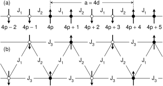
Figure 1: (a) 1D model of double-layered antiferromagnets in the linear chain structure. The spin arrangement is represented by the arrows (circles) which are upwards ($\bullet$) for $S^{z}=+S$ and downwards ($\circ$) for $-S$. The exchange integrals $J_{1}$ and $J_{2}$ are for the intra- (, ) and inter-sublattice () interactions, respectively. All sites have the same spacing $d$ and are indexed by $4p+n$, where $n=0$, 1, 2, and 3 in the $p$th unit cell. (b) 1D model of the railroad trestle type, possessing an additional exchange parameter $J_{3}$. Each site has one nearest neighbor (NN) of same spin (related by $J_{1}$) and three NNs of opposite spin (related by $J_{2}$ and $J_{3}$).

This study proceeds in the following steps. First, the magnonic equations for two one-dimensional (1D) models of double-layered antiferromagnets are solved in an accessible formulation. In Fig. 1, the model (a) represents a simple LC. Our treatment essentially follows what is standardly presented for ferro- and antiferro-magnons in textbooks, see e.g., Ref. [4]. The spin-paired arrangement is presently described within a four-atom unit cell with periodic boundary conditions. The ground state is assumed to be of Néel type and the paired spin configuration $|{+}{+}{-}{-}\rangle$ of $S^{z}=+S$ and $-S$ is assured by an alternation of two exchange parameters, the FM ($J_{1}>0$) and AFM ($J_{2}<0$) ones. For stabilization of the Néel state, a presence of additional weaker interactions, such as crystal anisotropy and next nearest neighbor exchange, might be anticipated. The model (b) represents a more complex 1D system that can be possibly named as railroad trestle (RT). Such a lattice reminds more closely the real situation in AFM CrN and includes now three exchange parameters, which can be under some condition all negative and of comparable strength, and still keeping the $|{+}{+}{-}{-}\rangle$ ground state stable. Once the equations of spin motion for LC and RT are solved and magnon dispersion relations determined, the model magnons are compared with ab initio calculations for real three-dimensional (3D) structure of AFM CrN.

Theoretical background—The first part of this letter has been devoted to the equations of spin motion under action of torque forces, which are required to solve the magnon spectra. Consider $N$ spins each of magnitude $S$ in 1D periodic cell. By adopting only the 1st nearest neighbor (NN) interactions, the Heisenberg Hamiltonian is written to be

$$\mathcal{H}=-2J\sum_{p=1}^{N}\mathbf{S}_{p}\cdot\mathbf{S}_{p+1}.$$ (1)

Here $\hbar\mathbf{S}_{p}$ is the spin angular momentum at site $p$. The interactions on the $p$th spin are

$$\mathcal{H}_{p}=-2J\mathbf{S}_{p}\cdot(\mathbf{S}_{p-1}+\mathbf{S}_{p+1})\equiv-\boldsymbol{\mu}_{p}\cdot\mathbf{B}_{p},$$ (2)

where $\boldsymbol{\mu}_{p}=-g\mu_{\text{B}}\mathbf{S}_{p}$ and $\mathbf{B}_{p}=-(2J/g\mu_{\text{B}})(\mathbf{S}_{p-1}+\mathbf{S}_{p+1})$ are the magnetic moment and effective magnetic field at site $p$, respectively. The time-dependent dynamics of $\hbar\mathbf{S}_{p}$ is defined by the torque $\boldsymbol{\mu}_{p}\times\mathbf{B}_{p}$ as

$$d\mathbf{S}_{p}/dt=(-g\mu_{\text{B}}/\hbar)\mathbf{S}_{p}\times\mathbf{B}_{p}.$$ (3)

At the final step, the ab initio calculations have been performed to realize our model analysis in AFM CrN. The local density approximation (LDA) [5] plus $U$ approach [6] is used with the projector augmented wave (PAW) potentials [7], implemented in vasp package [8, 9]. The crystal structure of AFM CrN (space group $Pnma$, No. 62) is fully optimized using $U=4.1$ eV for the $3d$ electrons at Cr sites. To explore the magnonic properties, a tight-binding model is constructed from the electronic structure using wannier90 library [10], including the Cr-$d$ and N-$p$ characters as a basis set. The magnetic exchange parameters $J_{ij}$ are extracted for neighboring Cr pairs with indices $i$ and $j$ given in the Hamiltonian

$$\mathcal{H}=-2\sum_{i>j}J_{ij}\mathbf{S}_{i}\cdot\mathbf{S}_{j},$$ (4)

by employing tb2j code [11] based on the local force theorem [12]. The magnon spectra are computed by applying the linear spin wave theory that is a plausible approximation for systems with larger spin, including the present one with $S=3/2$. The algorithm spinw [13] based on Holstein-Primakoff approximation of spin operators is used. The classical Monte-Carlo simulations are carried out with vampire software [14] to obtain the magnetization curve.

Model 1: Linear chain—We start with the simple 1D model of double-layered antiferromagnets as illustrated in Fig. 1(a). The spins of $S^{z}=+S$ and $-S$ are indicated by the filled ($\bullet$) and open ($\circ$) circles, respectively. The intra- and inter-sublattice interactions of $J_{1}$ and $J_{2}$ are implemented in Eq. (3) according to the geometry of Fig. 1(a). The spin indices are $4p+n$, where $n=0$, 1, 2, and 3 for the four magnetic sites in the $p$th unit cell. The lattice parameter is $a=4d$ with the same spacing $d$ for all sites. Let us focus on the case of $n=0$. By assuming $(S^{x},S^{y})\ll S$, we get the linearized equations in Cartesian components

$$\begin{split}dS_{4p}^{x}/dt&=(2S/\hbar)(\Delta JS_{4p}^{y}-J_{2}S_{4p-1}^{y}-J_{1}S_{4p+1}^{y}),\\ dS_{4p}^{y}/dt&=-(2S/\hbar)(\Delta JS_{4p}^{x}-J_{2}S_{4p-1}^{x}-J_{1}S_{4p+1}^{x}),\end{split}$$ (5)

with $\Delta J=J_{1}-J_{2}$. After repeating Eq. (5) for other three sites, the combined expressions from the ladder operation $S^{+}=S^{x}+iS^{y}$ are

$$\begin{split}dS_{4p}^{+}/dt&=-i(2S/\hbar)(\Delta JS_{4p}^{+}-J_{2}S_{4p-1}^{+}-J_{1}S_{4p+1}^{+}),\\ dS_{4p+1}^{+}/dt&=-i(2S/\hbar)(\Delta JS_{4p+1}^{+}-J_{1}S_{4p}^{+}-J_{2}S_{4p+2}^{+}),\\ dS_{4p+2}^{+}/dt&=i(2S/\hbar)(\Delta JS_{4p+2}^{+}-J_{2}S_{4p+1}^{+}-J_{1}S_{4p+3}^{+}),\\ dS_{4p+3}^{+}/dt&=i(2S/\hbar)(\Delta JS_{4p+3}^{+}-J_{1}S_{4p+2}^{+}-J_{2}S_{4p+4}^{+}),\end{split}$$ (6)

where the solutions of $S^{+}$ are traveling spin waves

$$S_{4p+n}^{+}=u_{n}\exp[i(4p+n)kd-i\omega t].$$ (7)

By substituting this into Eq. (6), four linear equations for wave function coefficients $u_{n}$ are obtained and become solvable for a specific dispersion $\omega(k)$. The magnon dispersion relation is acquired by solving the following determinant to be zero

$$\begin{array}[]{|cccc|}\Delta\omega-\omega&-\omega_{1}e^{ikd}&0&-\omega_{2}e^{-ikd}\\ -\omega_{1}e^{-ikd}&\Delta\omega-\omega&-\omega_{2}e^{ikd}&0\\ 0&-\omega_{2}e^{-ikd}&\Delta\omega+\omega&-\omega_{1}e^{ikd}\\ -\omega_{2}e^{ikd}&0&-\omega_{1}e^{-ikd}&\Delta\omega+\omega\end{array}=0,$$ (12)

which leads to secular equation

$$\omega^{4}-4(\omega_{1}^{2}-\omega_{1}\omega_{2})\omega^{2}+4\omega_{1}^{2}\omega_{2}^{2}\sin^{2}(2kd)=0,$$ (13)

where $\omega_{1,2}=(2S/\hbar)J_{1,2}$ and $\Delta\omega=\omega_{1}-\omega_{2}$. We get the spectrum of acoustic ($-$) and optical ($+$) modes

$$\omega(k)=\omega_{0}\sqrt{A\pm B(k)},$$ (14)

where $\omega_{0}=\sqrt{2|\omega_{1}\omega_{2}|}$ is the characteristic frequency and

$$\begin{split}A={}&(\operatorname{sgn}{\gamma})(\gamma-1),\\ B(k)={}&\sqrt{(\gamma-1)^{2}-\operatorname{\smash{\sin}}^{2}(2kd)},\end{split}$$ (15)

defining $\gamma=J_{1}/J_{2}$. To assure stability of the $|{+}{+}{-}{-}\rangle$ ground state, any imaginary solutions should be avoided. This gives the condition $\gamma<0$, which means that alternation of positive $J_{1}$ and negative $J_{2}$ is required.

The plot of $\omega(k)$ in Eq. (14) is shown in Fig. 2(a) for $\gamma=-1$ and $-1/3$. Each of the acoustic and optical branches are 2-fold degenerate (for illustration of spin wave modes and the double degeneracy associated with chirality see Appendix A), hence there are in total four magnon bands. A characteristic feature is the magnon gap at the Brillouin zone (BZ) boundary $k=\pi/a$. The gap is calculated to $\sqrt{2}\omega_{0}$ for $\gamma=-1$, while it vanishes for $\gamma\rightarrow 0^{-}$.

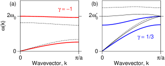
Figure 2: Selected magnon dispersion relations of double-layered antiferromagnets in the models of (a) linear chain and (b) railroad trestle (RT). Four types of lines indicate $\gamma=J_{1}/J_{2}=-1$ (red), $-1/3$ (black dashed), 0 (black solid), and $1/3$ (blue). The characteristic frequencies are $\omega_{0}=\sqrt{2|\omega_{1}\omega_{2}|}$ and $\omega_{0}^{\prime}=\sqrt{2}|\omega_{2}|$. Here, positive $\gamma$ of $1/3$ means all magnetic interactions in RT being antiferromagnetic.

Model 2: Railroad trestle—We solve another 1D model in Fig. 1(b), now considering both the FM $J_{1}$ and the less obvious case of AFM $J_{1}$. For simplicity, we take the other AFM parameters equal ($J_{2}=J_{3}<0$). The corresponding secular equation is shown in Appendix B. After going through a more complex process than for the LC above, we get the spectrum

$$\omega(k)=\omega_{0}^{\prime}\sqrt{C(k)\pm D(k)},$$ (16)

where $\omega_{0}^{\prime}=\sqrt{2}|\omega_{2}|$ is the characteristic frequency and

$$\begin{split}C(k)={}&(\gamma-2)(\gamma-1)+2\sin^{2}(2kd),\\ D(k)={}&\sqrt{(\gamma-2)[\gamma^{2}(\gamma-4)+(5\gamma-2)\cos^{2}(2kd)]}.\end{split}$$ (17)

The stability of the spin-paired arrangement in Fig. 1(b) is assured if calculated $\omega(k)$ become physically meaningful with $C(k)\pm D(k)\geq 0$ and real $D(k)$. This is fulfilled for the range of $\gamma$ from any negative value (FM $J_{1}$) to a positive limit of $\gamma=2/3$ (AFM $J_{1}$), i.e., in the interval $\gamma\leq 2/3$ ($J_{1}\geq-2|J_{2}|/3$). There is a finite magnon gap at the BZ boundary, but except for $\gamma=0$.

For illustration of magnon spectra we use a special case of $\gamma=0$, for which Eq. (16) can be simplified. The solution reduces to

$$\omega(k)=\begin{cases}2\omega_{0}^{\prime}|\sin kd|\sqrt{3-2\operatorname{\smash{\sin}}^{2}kd}&(\text{Acoustic}),\\ 2\omega_{0}^{\prime}|\cos kd|\sqrt{1+2\operatorname{\smash{\sin}}^{2}kd}&(\text{Optical}).\end{cases}$$ (18)

The dispersion relations of Eqs. (16) and (18) are illustrated in Fig. 2(b) for $\gamma=-1/3$, 0, and $1/3$.

Here we summarize our model analyses. The double-layered antiferromagnetism in LC is conditioned by an alternation of FM and AFM exchange integrals $(J_{1},J_{2})=({+|J_{1}|},{-|J_{2}|})$ with no restriction on the magnitudes of $J_{1}$ and $J_{2}$. Analogous magnetic arrangement in chain of RT geometry includes three exchange parameters of obvious combination $(J_{1},J_{2},J_{3})=({+|J_{1}|},{-|J_{2}|},{-|J_{3}|})$, but negative sign of $J_{1}$ is also permitted. In particular for $J_{2}=J_{3}$, the stability of the double-layered antiferromagnetism with $|{+}{+}{-}{-}\rangle$ unit cell, seen in Fig. 1(b), is assured down to $J_{1}=-2|J_{2}|/3$. For more negative $J_{1}$, there is a region of canted spin arrangements and finally for $J_{1}\leq-2|J_{2}|$, the stability of another double-layered antiferromagnetism with $|{+}{-}{-}{+}\rangle$ unit cell (see Appendix C). As magnetic excitations are concerned, the fundamental property of 1D double-layered antiferromagnets is the presence of acoustic and optical branches showing a magnon gap at the BZ boundary.

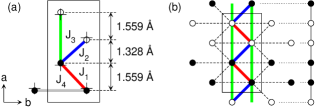
Figure 3: (a) The crystal structure and magnetic ordering of CrN projected to the orthorhombic $ab$ plane. The symbols “$\bullet$ ($\circ$)” and “$+$” indicate the Cr sites of $S^{z}=+S$ ($-S$) and N sites, respectively. Four kinds of magnetic exchange parameters $J_{1}$ (red), $J_{2}$ (blue), $J_{3}$ (green), and $J_{4}$ (grey) are marked. (b) Schematic two-dimensional picture of exchange links. The full lines denote the motif running along the $a$ axis that closely reminds the railroad trestle in Fig. 1(b) with magnetic exchange parameters $J_{1}$, $J_{2}$, and $J_{3}$. The dashed lines show links toward Cr atoms in neighboring unit that include in addition to $J_{1}$ and $J_{2}$, also a new parameter $J_{4}$. The projection to the $a$ axis, seen on the right side, refers to the spin-paired linear chain of Fig. 1(a).

Table 1: Summary of the distances $d_{ij}$ and magnetic exchange parameters $J_{ij}$ among the four kinds of nearest neighbor (NN) $i$-$j$ pairs, from the ab initio calculations with $U=4.1$ eV. We consider three variants of CrN structure by keeping the same volume of the magnetic unit cell. (i) The hypothetical cubic phase of rock-salt (RS) type. (ii) The intermediate structure upon orthorhombic distortion but without (w/o) local atomic shifts (AS). (iii) The real fully optimized orthorhombic phase with (w/) AS. The lattice parameters are $(a,b,c)=(\sqrt{2}c,c/\sqrt{2},c)=(5.8536,2.9268,4.1391)$ Å for (i) and $(a,b,c)=(5.7743,2.9647,4.1421)$ Å for (ii, iii). The atomic positions are specified by $(x_{\text{Cr}},1/4,1/4)$ for the Cr and $(x_{\text{N}},1/4,3/4)$ for the N sites, where $(x_{\text{Cr}},x_{\text{N}})=(1/8,1/8)$ for (i, ii) and $(x_{\text{Cr}},x_{\text{N}})=(0.1350,0.1146)$ for (iii). The intra-sublattice (SL) interaction of index $J_{4}$ arises in the three-dimension connecting the neighboring unit cells in the $b$ direction. The full list of the distance vectors is given by $\mathbf{d}_{ij}=\pm d_{ij}^{x}\hat{x}\ {\pm(\pm)(\mp)(\mp)}\ d_{ij}^{y}\hat{y}\ {\pm(\mp)(\pm)(\mp)}\ d_{ij}^{z}\hat{z}$.

Type	Index	Distance vector $\mathbf{d}_{ij}$			(i) Cubic RS		(ii) Ortho w/o AS		(iii) Ortho w/ AS
		${d}_{ij}^{x}$	${d}_{ij}^{y}$	${d}_{ij}^{z}$	$|d_{ij}|$ (Å)	$J_{ij}$ (meV)	$|d_{ij}|$ (Å)	$J_{ij}$ (meV)	$|d_{ij}|$ (Å)	$J_{ij}$ (meV)
Intra-SL	$J_{1}$	$2x_{\rm Cr}a$	$b/2$	$c/2$	2.9268	$-$2.6361	2.9275	$-$2.5951	2.9862	$-$0.2553
	$J_{4}$	0	$b$	0	2.9268	$-$2.4309	2.9647	$-$1.1701	2.9647	$-$1.0128
Inter-SL	$J_{2}$	$(1/2-2x_{\rm Cr})a$	$b/2$	$c/2$	2.9268	$-$2.9943	2.9275	$-$2.9516	2.8724	$-$4.9555
	$J_{3}$	$a/2$	0	0	2.9268	$-$2.6247	2.8872	$-$3.7028	2.8872	$-$3.5406

Antiferromagnetic CrN—To verify the validity of the preceding analyses in real materials, the ab initio calculations for AFM CrN have been performed precisely. Important values of exchange integrals are found namely for the NN Cr-Cr pairs ($d\approx 2.9$ Å), while those for Cr-N-Cr ($\approx 4.1$ Å) and farther pairs are negligible. Concerning the global effect of these NN exchange integrals, it should be noted the Cr atoms in the orthorhombically distorted rock-salt structure form a lattice close to the face-centered cubic (fcc) one. In absence of the structural distortion, which is the situation in paramagnetic state above the magnetostructural transition [1], there are twelve symmetry-equivalent and AFM (negative $J$) NN links. This would lead to highly frustrated magnetic interactions. To understand the observed double-layered arrangement of CrN and its stability [2, 3], the effects of both the macroscopic lattice distortion and local atomic displacements should be taken in account. As seen in the projection of AFM CrN to the orthorhombic $ab$ plane in Fig. 3(a), there are two oppositely oriented magnetic sublattices formed by double $bc$ layers of Cr atoms with spacing of 1.559 Å, while the inter-sublattice spacing of the layers is smaller and makes 1.328 Å [*[Formoredetailedstructuraldescriptionsee][.]Ahn2024]. Fig. 3(b) then illustrates exchange links in AFM CrN in a two-dimensional (2D) scheme that shows clear similarity to the 1D model of RT treated above. Each Cr atom has four NNs in neighboring layer of same spin (exchange integral $J_{1}$), four NNs in opposite neighboring layer with reversed spin ($J_{2}$), two NNs in next layers ($J_{3}$), and two NNs within the same layer ($J_{4}$). These four kinds of NN pairs of Cr sites are diversified by interatomic distances and much markedly, by theoretically calculated values of corresponding exchange integrals. Three structural variants have been considered: (i) the hypothetical cubic rock-salt structure, (ii) the macroscopically distorted one, and lastly, (iii) the real CrN structure, i.e., including the local atomic shifts. The respective results are provided in Table 1. An illustrative summary is presented in Fig. 4, showing a clear correlation of exchange integrals on the Cr-Cr NN distances.

It appears that the gradual diversification of the NN Cr-Cr distances leads eventually to a remarkable difference between the inter-sublattice integrals $(J_{2},J_{3})=({-4.9555},{-3.5406})~\text{meV}\ll 0$ and intra-sublattice ones $(J_{1},J_{4})=({-0.2553},{-1.0128})~\text{meV}\lesssim 0$, keeping all of them negative. Let us note that the largest value found for $J_{2}$ is in good agreement with Ref. [16]. Fig. 5(b) displays the calculated temperature dependence of the local magnetic moments. Néel temperature has been determined to $T_{\text{N}}=284$ K, which is consistent with the reported experimental value of 287 K [1], proving that our $J$ values are reasonable.

Figure 4: Calculated magnetic exchange parameters for three variants of CrN structure: (purple squares) the hypothetical cubic phase of rock-salt (RS) type, (empty triangles) the intermediate structure upon orthorhombic distortion but without (w/o) local atomic shifts (AS), and (black dots with $J_{1}$, …, $J_{4}$ denoted) the real fully optimized orthorhombic phase with (w/) AS. The dashed line shows nearly linear dependence of the exchange parameters on the distance between nearest neighbor Cr pairs.

The 2D array of exchange links in Fig. 3(b) is only a simplified illustration of the 3D array existing in real CrN. To calculate the magnon spectra of AFM CrN, the ab initio determined isotropic exchange interactions $J_{1}$, …, $J_{4}$ have been used for construction of magnetic Hamiltonian and subsequent transformation of spin excitations to bosonic operators. The resulting dispersion relations are presented in Fig. 5(a). Since double-layered AFM arrangement holds along the crystallographic $a$ direction while the FM order is maintained along the $b$ and $c$ directions, the magnon gap appears only at the X point but not for the Y and Z points.

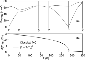
Figure 5: (a) Magnon dispersion relation of antiferromagnetic CrN. The presence of magnon gap at the X point shows a good agreement with the model analysis in Fig. 2. (b) Calculated magnetization curve from the classical Monte-Carlo simulations. The ordering temperature of $T_{\text{N}}=284$ K was obtained by fitting with $(1-T/T_{\text{N}})^{\beta}$ and $\beta=1/3$.

Conclusions—The factors ensuring the double-layered AFM order to be stable have been investigated for two models of 1D character and periodic conditions, the LC and more complex chain of RT geometry. In the next part, detailed ab initio calculations have been performed for real solid system represented by chromium nitride of CrN composition. As the LC is concerned, the spin-paired order $|{+}{+}{-}{-}\rangle$ requires necessarily some at least weak FM coupling for intra-sublattice pairs (, ) while that for inter-sublattice () is naturally AFM. On the other hand, the geometry of RT allows for presence of some frustration, and in this model, the intra-sublattice pairing can be stable even for all exchange interactions AFM if certain conditions are fulfilled. Solving the equations of spin motion for these 1D models, it is found that applying the isotropic Heisenberg Hamiltonian to spin-paired magnetic order, doubly degenerate acoustic and optical magnon modes with gap between them at BZ boundary are obtained. The degeneracy refers to magnon pairs of opposite chirality, the presence of which is characteristic for antiferromagnets.

As crystal structure of CrN is concerned, it derives from a common rock-salt type. Its orthorhombic lattice distortion below Néel temperature points to a complex contribution of Cr-Cr and Cr-N-Cr chemical bonds, in which the spin polarization of bonding electrons plays a role. The AFM ordering is formed by FM double-layers in the orthorhombic $bc$ plane (the pseudocubic $(110)$ plane) that are stacked in the $|{+}{+}{-}{-}\rangle$ order along the $a$ direction. There are four kinds of magnetic links Cr-Cr, two exchange parameters for intra-sublattice pairs and two for inter-sublattice ones. While all these links would be equivalent for hypothetical cubic structure of CrN, the lattice distortion and especially the associated shifts of fractional Cr positions diversify the distances among Cr NNs. As a result, we find marked differences between the inter-sublattice parameters $(J_{2},J_{3})\ll 0$ and intra-sublattice ones $(J_{1},J_{4})\lesssim 0$. The stability of the double-layered AFM ordering is thus attained in CrN, even if the intra-sublattice interactions remain all AFM.

Acknowledgments—S.-J. K. gratefully acknowledges studentship support from the International Max Planck Research School for Chemistry and Physics of Quantum Materials. This work was supported by Grants No. 22-10035K, No. 23-04746S, and No. 25-17490S of the Czech Science Foundation and Grant No. 471878653 of the German Research Foundation. Computational resources were provided by e-INFRA CZ Grant No. 90254. We further acknowledge the Operational Program Research, Development and Education financed by the European Structural and Investment Funds and by the Ministry of Education, Youth and Sports of the Czech Republic, Grant No. CZ.02.01.01/00/22_008/0004594 (TERAFIT).

Data availability—Data associated with this study are available on the Zenodo repository [17].

Appendices

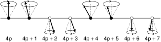
Figure 6: Semiclassical picture of acoustic magnon in the $|{+}{+}{-}{-}\rangle$ linear chain. Here the phase shifts between the nearest neighbor sites are set $kd=30$° with $\alpha=\beta=0$ for better visibility. The bold vectors show an instantaneous orientation of atomic spins for magnon propagating along the horizontal right direction with positive $k$.

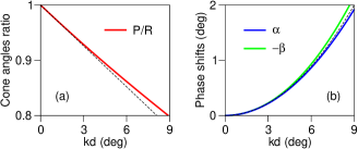
Figure 7: Spin wave parameters (red) $P/R$, (blue) $\alpha$, and (green) $-\beta$ at the small $k$ regime up to $kd=9$°, which corresponds to $k=0.2\pi/a$. The dashed lines in (a) and (b) indicate the leading terms $1-\sqrt{2}kd$ and $\sqrt{2}(kd)^{2}$, respectively.

Appendix A: Spin waves in LC model—Within present approximation valid for $(S^{x},S^{y})\ll S$, the spin dynamics of the LC with collinear $|{+}{+}{-}{-}\rangle$ order seen in Fig. 1(a) is described by Eqs. (6) and (7). The solution for given reciprocal vector $k$ gives four traveling spin waves of the conical spiral form: two degenerate acoustic modes and two degenerate optical ones. An example of the acoustic mode is schematically shown in Fig. 6. This magnon is characterized with larger cone angles for spin-up sites and clockwise rotations of local spins (positive $\omega$), while its degenerate counterpart possessing opposite chirality would display exactly reversed cone angles and counter-clockwise rotation of atomic spins (negative $\omega$). Such a situation is analogous to what was discussed in detail for simple $|{+}{-}{+}{-}\rangle$ chain by Keffer et al. [18]. It should be noted that in the present $|{+}{+}{-}{-}\rangle$ chain with four magnetic sites $n=0$, 1, 2, and 3, the calculated spin wave parameters $u_{0}$, $u_{1}$, $u_{2}$, and $u_{3}$ are generally of complex values. This means that phase shifts $\varphi$ between neighboring sites are not regular ($\varphi=kd$) as Eq. (7) seems to suggest, but they are diversified for the spin-up pairs, spin-down pairs, and spin-antiparallel pairs.

Fig. 7 summarizes the spin wave parameters, calculated for special case of $\gamma=-1$ and expressed suitably in a polar form $u_{0(1)}=R\exp[+(-)i\alpha/2]$ and $u_{2(3)}=-P\exp[+(-)i\beta/2]$. It appears that the ratio of the spin-down and spin-up cone angles decreases with increasing $k$ as $P/R\simeq 1-\sqrt{2}kd+(kd)^{2}$. The additional phase shifts $\alpha$ ($\beta$) between spin-up (spin-down) pairs have opposite signs and show essentially the quadratic dependence on $k$ as $\alpha~(\beta)\simeq+(-)\sqrt{2}(kd)^{2}-(kd)^{3}/2$. The actual phase shift between spin-up pairs is thus decreased (to $\varphi=kd-\alpha$), and that between spin-down pairs is similarly increased.

Appendix B: Equations of motion for the spin chain of RT type—We consider the dynamics of the RT model in Fig. 1(b). In distinction to Eq. (3) for simple LC, the torque acting on spins in RT includes two more terms due to larger number of NN spins. There are again four equations of spin motion in local ladder operators

$$\begin{split}dS_{4p}^{+}/dt&=-i(2S/\hbar)[\Delta JS_{4p}^{+}-J_{2}S_{4p-1}^{+}-J_{1}S_{4p+1}^{+}\\ &\phantom{=-i(2S/\hbar)[}-J_{3}(S_{4p-2}^{+}+S_{4p+2}^{+})],\\ dS_{4p+1}^{+}/dt&=-i(2S/\hbar)[\Delta JS_{4p+1}^{+}-J_{1}S_{4p}^{+}-J_{2}S_{4p+2}^{+}\\ &\phantom{=-i(2S/\hbar)[}-J_{3}(S_{4p-1}^{+}+S_{4p+3}^{+})],\\ dS_{4p+2}^{+}/dt&=i(2S/\hbar)[\Delta JS_{4p+2}^{+}-J_{2}S_{4p+1}^{+}-J_{1}S_{4p+3}^{+}\\ &\phantom{=i(2S/\hbar)[}-J_{3}(S_{4p}^{+}+S_{4p+4}^{+})],\\ dS_{4p+3}^{+}/dt&=i(2S/\hbar)[\Delta JS_{4p+3}^{+}-J_{1}S_{4p+2}^{+}-J_{2}S_{4p+4}^{+}\\ &\phantom{=i(2S/\hbar)[}-J_{3}(S_{4p+1}^{+}+S_{4p+5}^{+})],\end{split}$$ (B1)

where $\Delta J=J_{1}-J_{2}-2J_{3}$ and the same solutions for $u_{n}$ with Eq. (7). The magnon dispersion relation is obtained by solving

$$\begin{array}[]{|cccc|}\Delta\omega-\omega&-\omega_{1}e^{ikd}&f_{3}(k)&-\omega_{2}e^{-ikd}\\ -\omega_{1}e^{-ikd}&\Delta\omega-\omega&-\omega_{2}e^{ikd}&f_{3}(k)\\ f_{3}(k)&-\omega_{2}e^{-ikd}&\Delta\omega+\omega&-\omega_{1}e^{ikd}\\ -\omega_{2}e^{ikd}&f_{3}(k)&-\omega_{1}e^{-ikd}&\Delta\omega+\omega\end{array}=0,$$ (B6)

where $\omega_{1,2,3}=(2S/\hbar)J_{1,2,3}$, $\Delta\omega=\omega_{1}-\omega_{2}-2\omega_{3}$, and $f_{3}(k)=-2\omega_{3}\cos(2kd)$. The analytical solution is possible only for special combination of exchange parameters $J_{1}$, $J_{2}$, and $J_{3}$, see e.g., Eq. (16) for $J_{2}=J_{3}$.

Appendix C: Stability of collinear AFM states in the RT model—Taking into account magnetic frustration at all negative $J_{1}$, $J_{2}$, and $J_{3}$ in the RT model, we consider the conditions for stability of three collinear arrangements: the discussed double-layered AFM2 with four-atom unit cell $|{+}{+}{-}{-}\rangle$ seen in Fig. 1(b), its spin modification AFM2^′ with unit cell $|{+}{-}{-}{+}\rangle$, and the standard single-layered AFM1 with unit cell $|{+}{-}{+}{-}\rangle$. Their respective energies are $E_{\text{AFM2}}=4(-J_{1}+J_{2}+2J_{3})S^{2}$, $E_{\text{AFM2}^{\prime}}=4(J_{1}-J_{2}+2J_{3})S^{2}$, and $E_{\text{AFM1}}=4(J_{1}+J_{2}-2J_{3})S^{2}$. The conventional spin alternation $|{+}{-}{+}{-}\rangle$ of AFM1 is stabilized when the strengths of negative-valued $J_{1}$ and $J_{2}$ dominate over the $J_{3}$ one. Our interest is, nonetheless, in the special case of $J_{2}=J_{3}<0$, for which the RT model gives results similar to behavior of the real CrN. It is obvious that for $J_{1}\geq 0$ ($\gamma\leq 0$) there is no frustration, and the collinear $|{+}{+}{-}{-}\rangle$ arrangement is the real ground state, and intuitively, one may expect it stable even for some negative and small $J_{1}$. Clear frustration occurs for $J_{1}=J_{2}$, for which $E_{\text{AFM2}}=E_{\text{AFM2}^{\prime}}$. For more negative $J_{1}<-|J_{2}|$ ($\gamma>1$), the AFM2^′ with shifted spin order $|{+}{-}{-}{+}\rangle$ is of the lowest energy among the three.

Figure 8: The stability of collinear magnetic arrangements of railroad trestle. Exchange parameters $J_{2}$ and $J_{3}$ are considered to be antiferromagnetic (AFM) and equal ($J_{2}=J_{3}<0$), while $J_{1}$ varies from ferromagnetic (FM) to AFM. Lower axis denotes the values of $\gamma=J_{1}/J_{2}$. The region of AFM2 with $|{+}{+}{-}{-}\rangle$ unit cell is characterized by magnon spectra for $\gamma=-2/3$ and $2/3$ (see Fig. 2(b) for $\gamma=-1/3$, 0, and $1/3$), and that of AFM2^′ with $|{+}{-}{-}{+}\rangle$ unit cell by spectra for $\gamma=2$ and 3. The characteristic frequency is $\omega_{0}^{\prime}=\sqrt{2}|\omega_{2}|$. In the middle part, the calculations of acoustic branches for AFM2/AFM2^′ magnons give non-physical solutions, which suggests that there should be a region of non-collinear (NC) ground states.

Since there is a possibility of non-collinear arrangements, the range of true AFM2/AFM2^′ stability has been investigated. Let us move our focus from $E(J,S)$ to $\omega(k)$. Fig. 8 shows the calculated magnon spectra for both double-layered arrangements at $J_{2}=J_{3}<0$. In the $2/3<\gamma<2$ region, the results reveal imaginary solutions for some range of $\omega(k)$ for acoustic magnons, which indicates the non-stability of both the $|{+}{+}{-}{-}\rangle$ and $|{+}{-}{-}{+}\rangle$ configurations and suggests for non-collinear ground states. On the other hand, it is confirmed that the AFM2 arrangement of current interest represents a ground state for any positive $J_{1}$ ($\gamma<0$) and also for small negative one ($0\leq\gamma\leq 2/3$). The stability region for alternative AFM2^′ is found for negative $J_{1}$ dominating over $J_{2}$ and $J_{3}$ ($\gamma\geq 2$).

As a final comment, it should be noted that present semiclassical approach to AFM ground states and their magnon dynamics is appropriate only for atomic moments of larger spin values. For small spins, in particular $S=1/2$, a more complex quantum mechanical solution is needed. The spin arrangements of Néel type have been thus shown not to be the true eigenstates of isotropic Heisenberg Hamiltonian for AFM exchange integral $J$. The solutions for LCs with periodic condition can be found in very instructive paper of Bonner and Fisher [19]. Taking different Néel configurations (alternations of atomic spins $S^{z}=\pm 1/2$) as basis vectors, it is shown that AFM eigenstates are linear combinations of all basis vectors with zero total spin, irrespective the length of unit cell. For the four-atom unit cell, the ground state for simple linear AFM chain is formed by a linear combination of $|{+}{-}{+}{-}\rangle$, $|{-}{+}{-}{+}\rangle$, $|{+}{+}{-}{-}\rangle$, $|{-}{-}{+}{+}\rangle$, $|{+}{-}{-}{+}\rangle$, and $|{-}{+}{+}{-}\rangle$. Findings for variable unit cell (up to $N=12$) demonstrate the absence of long range magnetic order in the AFM chain, and the extrapolated energy of the ground state corresponds to the exact value of $-2N|J|(\ln{2}-1/4)=-0.88629N|J|$ that has been derived in famous paper of Bethe [20]. Compared to FM chain and its quantum mechanical energy of $-2NJS^{2}$ for any $S$ value, the energy of AFM chain for $S=1/2$ can be formally written as $-2N|J|S(S+0.38629)$.

References

- Wang et al. [2023] L. Wang, W. Xu, X. Zhou, C. Gu, H. Cheng, J. Chen, L. Wu, J. Zhu, Y. Zhao, E.-J. Guo, and S. Wang, Phys. Rev. B 107, 174112 (2023).
- Corliss et al. [1960] L. M. Corliss, N. Elliott, and J. M. Hastings, Phys. Rev. 117, 929 (1960).
- Gui et al. [2022] Z. Gui, C. Gu, H. Cheng, J. Zhu, X. Yu, E. Guo, L. Wu, J. Mei, J. Sheng, J. Zhang, J. Wang, Y. Zhao, L. Bellaiche, L. Huang, and S. Wang, Phys. Rev. B 105, L180101 (2022).
- Kittel [2004] C. Kittel, Introduction to Solid State Physics, 8th ed. (Wiley, New York, 2004).
- Ceperley and Alder [1980] D. M. Ceperley and B. J. Alder, Phys. Rev. Lett. 45, 566 (1980).
- Dudarev et al. [1998] S. L. Dudarev, G. A. Botton, S. Y. Savrasov, C. J. Humphreys, and A. P. Sutton, Phys. Rev. B 57, 1505 (1998).
- Kresse and Joubert [1999] G. Kresse and D. Joubert, Phys. Rev. B 59, 1758 (1999).
- Kresse and Furthmüller [1996a] G. Kresse and J. Furthmüller, Comput. Mater. Sci. 6, 15 (1996a).
- Kresse and Furthmüller [1996b] G. Kresse and J. Furthmüller, Phys. Rev. B 54, 11169 (1996b).
- Mostofi et al. [2014] A. A. Mostofi, J. R. Yates, G. Pizzi, Y.-S. Lee, I. Souza, D. Vanderbilt, and N. Marzari, Comput. Mater. Sci. 185, 2309 (2014).
- He et al. [2021] X. He, N. Helbig, M. J. Verstraete, and E. Bousquet, Comput. Phys. Commun. 264, 107938 (2021).
- Liechtenstein et al. [1984] A. I. Liechtenstein, M. I. Katsnelson, and V. A. Gubanov, J. Phys. F: Met. Phys. 14, L125 (1984).
- Toth and Lake [2015] S. Toth and B. Lake, J. Phys.: Condens. Matter 27, 166002 (2015).
- Evans et al. [2014] R. F. L. Evans, W. J. Fan, P. Chureemart, T. A. Ostler, M. O. A. Ellis, and R. W. Chantrell, J. Phys.: Condens. Matter 26, 103202 (2014).
- Ahn et al. [2024] K.-H. Ahn, Z. Jirák, J. Hejtmánek, and K. Knížek, Solid State Sci. 148, 107413 (2024).
- Biswas et al. [2023] B. Biswas, S. Rudra, R. S. Rawat, N. Pandey, S. Acharya, A. Joseph, A. I. K. Pillai, M. Bansal, M. de h-Óra, D. P. Panda, A. B. Dey, F. Bertram, C. Narayana, J. MacManus-Driscoll, T. Maity, M. Garbrecht, and B. Saha, Phys. Rev. Lett. 131, 126302 (2023).
- Kim et al. [2024] S.-J. Kim, Z. Jirák, J. Hejtmánek, K. Knížek, H. Rosner, and K.-H. Ahn, 10.5281/zenodo.14231969 (2024).
- Keffer et al. [1953] F. Keffer, H. Kaplan, and Y. Yafet, Am. J. Phys. 21, 250 (1953).
- Bonner and Fisher [1964] J. C. Bonner and M. E. Fisher, Phys. Rev. 135, A640 (1964).
- Bethe [1931] H. Bethe, Z. Phys. 71, 205 (1931).