Clustering-induced localization of quantum walks on networks

Abstract

Quantum walks on networks are a paradigmatic model in quantum information theory. Quantum-walk algorithms have been developed for various applications, including spatial-search problems, element-distinctness problems, and node centrality analysis. Unlike their classical counterparts, the evolution of quantum walks is unitary, so they do not converge to a stationary distribution. However, it is important for many applications to understand the long-time behavior of quantum walks and the impact of network structure on their evolution. In the present paper, we study the localization of quantum walks on networks. We demonstrate how localization emerges in highly clustered networks that we construct by recursively attaching triangles, and we derive an analytical expression for the long-time inverse participation ratio that depends on products of eigenvectors of the quantum-walk Hamiltonian. Building on the insights from this example, we then show that localization also occurs in Kleinberg navigable small-world networks and Holme–Kim power-law cluster networks. Our results illustrate that local clustering, which is a key structural feature of networks, can induce localization of quantum walks.

Quantum walks have numerous and diverse applications, including spatial-search problems [1, 2, 3, 4], element-distinctness problems [5], and computations of node centralities [6, 7, 8, 9, 10, 11, 12]. Potential applications of quantum walks extend well beyond these examples, as any problem that can be solved by a general-purpose quantum computer can also be implemented as a quantum walk on a network [13, 14]. Quantum walks are also effective models of various transport processes, such as energy transport in photosynthetic complexes [15, 16]. Unlike classical random walks, quantum walks evolve unitarily and thus do not converge to a stationary distribution. To mathematically characterize the evolution of quantum walks, one usually considers long-time means of quantities such as occupation and transition probabilities. Examining the long-time behavior of quantum walks and the influence of network structure on their evolution can help guide the integration of quantum walks into algorithms [17].

Dynamical processes on networks can exhibit localization, which occurs when they are eventually confined to a small set of nodes of a network [18, 19, 20, 21]. Localization arises from the interplay between a network’s structural properties and dynamical processes on it. In the present paper, we study the localization of continuous-time quantum walks (CTQWs) on networks.

Prior research on CTQWs has illustrated that adding edges uniformly at random to a ring network with nearest-neighbor connections is associated with ensemble-averaged transition probabilities that are large for an initially excited node (i.e., a single node that is initially occupied) and close to 0 for the other nodes [22]. Individual realizations of quantum walks on such networks do not exhibit localization. Averaging across different instantiations of the random process of adding edges is associated with transitions of an initial excitation of one node to any other node. These transitions tend to cancel each other out, causing excitations to remain localized on average in their initial location. Researchers have observed localization of individual quantum walks in tree networks with Hamiltonians that incorporate disorder [23, 24]. Relatedly, local connectivity patterns that are associated with $0$ eigenvalues have been identified with quantum-walk localization [25]. It is also known that quadratic perturbations can induce localization of quantum walks [26].

There is also a body of work on discrete-time quantum walks on networks. These studies include many papers [27, 28, 29, 30, 31, 31, 32, 33, 34, 35, 36, 37, 38] on localization involving both various lattices (and a fractal network) and “coin operators”, which act on the spin component of an underlying product state.

To study the localization of CTQWs on networks, we first establish how localization emerges in highly clustered networks that we construct by recursively attaching triangles. We then build on this example to show that localization also occurs in Kleinberg navigable small-world networks [39] and Holme–Kim power-law cluster networks [40]. These localization effects have potential implications for the use of quantum walks in quantum memory, where localized walks help reduce the size of the position space that is needed to store information [41]. Our results also illustrate how structural characteristics of networks can suppress the speed-ups of quantum-walk propagation over classical-walk propagation on networks, a factor that is relevant when employing quantum walks in quantum communication channels [23].

Quantum walks on networks.

Figure 1: Localization in recursive triangle networks. (a) Recursive triangle networks of depths 1, 2, and 3. The long-time mean inverse participation rations (IPRs) of the nodes with red rings are substantially larger than those of other nodes. (b) The long-time mean transition probabilities $\bar{\pi}_{ij}$ [see Eq. (4)] for the networks in (a). (c) The long-time mean IPR $\hbox{\vbox{\hrule height=0.5pt\kern 2.15277pt\hbox{\kern-0.50003pt$\mathrm{IPR}$\kern-1.49994pt}}}_{j}$ [see Eq. (7)] as a function of the node $j$ with an initial excitation. The hollow red circles indicate the maximum value of $\hbox{\vbox{\hrule height=0.5pt\kern 2.15277pt\hbox{\kern-0.50003pt$\mathrm{IPR}$\kern-1.49994pt}}}_{j}$. (d) The probability density $|\psi_{i}(t)|^{2}=|\braket{i}{\psi(t)}|^{2}$ as a function of the node $i$ and time $t$ for a CTQW that starts at node 61 in a recursive triangle network of depth 6. In this example, the quantum walker predominantly alternates between two nodes.

We consider unweighted, undirected networks in the form of graphs $G=(V,E)$, where $V$ is a set of nodes and $E$ is a set of edges. The number of nodes is $N=|V|$, and the number of edges is $M=|E|$. We describe the edges between nodes using an adjacency matrix $A\in\{0,1\}^{N\times N}$. The element $a_{ij}$ of the matrix $A$ is $1$ if nodes $i$ and $j$ are adjacent to each other and $0$ if they are not. Because the network is undirected, $a_{ij}=a_{ji}$. The degree of a node $i$ is $k_{i}=\sum_{j=1}^{N}a_{ij}$. Unless we state otherwise, we do not consider self-edges (i.e., we set $a_{ii}=0$).

The wave function $\ket{\psi}\in\mathbb{C}^{N}$ of a CTQW evolves according to the Schrödinger equation

$$\frac{\mathrm{d}}{\mathrm{d}t}\ket{\psi(t)}=-\mathrm{i}H\ket{\psi(t)}\,,$$ (1)

where $\mathrm{i}=\sqrt{-1}$ is the imaginary unit and the Hamiltonian $H$ is the infinitesimal generator of time translation. We assume the normalization $\braket{\psi(t)}{\psi(t)}=1$. In accordance with Refs. [42, 9, 10], we let $H$ be the symmetric and normalized graph Laplacian. That is,

$$H=D^{-1/2}LD^{-1/2}\,,$$ (2)

where $D=\sum_{j=1}^{N}k_{j}\ket{j}\bra{j}$ is the degree matrix and $L=D-A$ is the combinatorial graph Laplacian matrix. The quantity $\ket{j}\in\mathbb{C}^{N}$ is an orthonormal basis vector that satisfies $\braket{i}{j}=\delta_{ij}$, where $\delta_{ij}$ denotes the Kronecker delta, which is $1$ if $\ket{i}=\ket{j}$ and is $0$ otherwise. For the choice (2) of $H$, if a system is in the ground state, then the probability of finding a quantum walker on a given node is the same as in a classical random walk with the generator $LD^{-1}$ [42].

Localization measures.

The probability that a CTQW with Hamiltonian $H$ transitions from node $j$ at time $0$ to node $i$ at time $t$ is

$$\begin{split}\pi_{ij}(t)&=|\braket{i}{e^{-\mathrm{i}Ht}}{j}|^{2}\\ &=\sum_{m=1}^{N}A^{ij}_{m}+\sum_{m<n}B^{ij}_{mn}\cos((\lambda_{m}-\lambda_{n})t)\,,\end{split}$$ (3)

where $A^{ij}_{m}\coloneqq|\braket{i}{e_{m}}\braket{e_{m}}{j}|^{2}$ and $B^{ij}_{mn}\coloneqq 2\braket{i}{e_{m}}\braket{e_{m}}{j}\braket{j}{e_{n}}\braket{e_{n}}{i}$. The quantities $\lambda_{m}$ and $e_{m}$, respectively, are the eigenvalues and corresponding eigenvectors of $H$. That is, $He_{m}=\lambda_{m}e_{m}$. The long-time mean of the transition probability $\pi_{ij}(t)$ is

$$\bar{\pi}_{ij}=\lim_{T\rightarrow\infty}\frac{1}{T}\int_{0}^{T}\pi_{ij}(t)\,\mathrm{d}t\,.$$ (4)

Inserting Eq. (3) into Eq. (4) yields

$$\bar{\pi}_{ij} =\sum_{m=1}^{N}A^{ij}_{m}+\sum_{\begin{subarray}{c}m<n\,,\\ \lambda_{m}=\lambda_{n}\end{subarray}}B^{ij}_{mn}\,.$$ (5)

To quantify the amount of localization of a CTQW, we calculate the inverse participation ratio (IPR) [43, 44]

$$\mathrm{IPR}_{j}(t)=\sum_{i=1}^{N}|\braket{i}{e^{-\mathrm{i}Ht}}{j}|^{4}=\sum_{i=1}^{N}\pi_{ij}^{2}(t)$$ (6)

that associated with the initial state $\ket{j}$. To interpret the IPR, consider a wave function in which $\ell$ elements have a magnitude of $1/\sqrt{\ell}$ and $N-\ell$ elements have a magnitude of $0$. This wave function has an IPR of $\ell(1/\sqrt{\ell})^{4}=1/\ell$. Therefore, for a fully localized state, in which a CTQW is localized at a single node (i.e., $\ell=1$), the IPR attains its maximum value of $1$. For a fully delocalized state (i.e., $\ell=N$), the IPR attains its minimum value of $1/N$.

The long-time mean of $\mathrm{IPR}_{j}(t)$ is

$$\begin{split}\hbox{\vbox{\hrule height=0.5pt\kern 2.15277pt\hbox{\kern-0.50003pt$\mathrm{IPR}$\kern-1.49994pt}}}_{j}&=\lim_{T\rightarrow\infty}\frac{1}{T}\int_{0}^{T}\mathrm{IPR}_{j}(t)\,\mathrm{d}t\\ &=\sum_{i=1}^{N}\Big{[}\Big{(}\sum_{m=1}^{N}A^{ij}_{m}\Big{)}^{2}+2\sum_{m=1}^{N}A^{ij}_{m}\sum_{\begin{subarray}{c}m<n\,,\\ \lambda_{m}=\lambda_{n}\end{subarray}}B^{ij}_{mn}+\sum_{\begin{subarray}{c}m<n\,,\,r<s\,,\\ \lambda_{m}-\lambda_{n}=\lambda_{r}-\lambda_{s}\end{subarray}}C_{mnrs}^{ij}+\sum_{\begin{subarray}{c}m<n\,,\,r<s\,,\\ \lambda_{m}-\lambda_{n}=\lambda_{s}-\lambda_{r}\end{subarray}}C_{mnrs}^{ij}\Big{]}\,,\end{split}$$ (7)

where $C_{mnrs}^{ij}=B^{ij}_{mn}B^{ij}_{rs}/2$.

Localization in recursive triangle networks.

As a starting point, we examine recursive triangle networks [see Fig. 1(a)]. For a given depth $d$, such networks have $N=3\times 2^{d}$ nodes and $M=3\times(2^{d+1}-1)$ edges. In Fig. 1(a), we show recursive triangle networks with depths of $d=1$, $d=2$, and $d=3$. The mean clustering coefficients for these networks are 0.75, 0.71, and 0.70, respectively. For larger values of $d$, the mean clustering coefficient approaches a value of approximately 0.69.

For the networks with depths $d=1$, $d=2$, and $d=3$, we show the long-time mean transition-probability elements $\bar{\pi}_{ij}$ for all $i,j\in\{1,\dots,N\}$ in Fig. 1(b). For a recursive triangle network with depth $d=1$, one can obtain analytical expressions for the eigenvalues and eigenvectors of the Hamiltonian (2). This enables one to write down the long-time mean transition-probability matrix

$$\bar{\boldsymbol{\pi}}^{(d=1)}=\frac{1}{27}\begin{pmatrix}11&2&2&4&4&4\\ 2&11&2&4&4&4\\ 2&2&11&4&4&4\\ 4&4&4&11&2&2\\ 4&4&4&2&11&2\\ 4&4&4&2&2&11\\ \end{pmatrix}\,.$$ (8)

All diagonal elements $\bar{\pi}_{ii}^{(d=1)}$ have the same value and are much larger than the off-diagonal elements $\bar{\pi}_{ij}^{(d=1)}$ (with $i\neq j$). This indicates that a CTQW that starts at node $j$ has a higher probability of revisiting node $j$ over a long time horizon than of occupying any other node. For recursive triangle networks with depths of 2 and 3, over a long time horizon, CTQWs that start from nodes 4–6 and 7–12, respectively, have higher probabilities of revisiting these nodes than of occupying any other node [see Fig. 1(b)].

In Figs. 1(a,c), we highlight nodes with hollow red circles when their long-time mean IPRs [see Eq. (7)] are much larger than those of other nodes. For the recursive triangle network with depth $d=1$, nodes 1–3 have a long-time mean IPR of $269/729\approx 0.37$ and nodes 4–6 have a long-time mean IPR of $301/729\approx 0.41$. For the recursive triangle networks with depths 2 and 3, observe that the nodes with the largest long-time mean IPRs are the nodes with the largest diagonal elements of $\bar{\pi}_{ij}$ in Fig. 1(b).

The Hamiltonian $H$ of the recursive triangle network with depth $d=1$ has eigenvalues 0, 3/4, 3/4, 3/2, 3/2, and 3/2. The degeneracy of the eigenvalues 3/4 and 3/2 is associated with substantial contributions of the sums over $B_{mn}^{ij}$ for $\lambda_{m}=\lambda_{n}$. The sums over $C_{mnrs}^{ij}$ also contribute substantially to the overall long-time mean IPR, as several eigenvalue quadruplets satisfy $\lambda_{m}-\lambda_{n}=\lambda_{s}-\lambda_{r}$ and $\lambda_{m}-\lambda_{n}=\lambda_{r}-\lambda_{s}$. We observe similar characteristics in recursive triangle networks with larger depths.

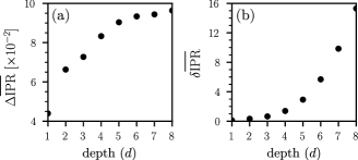
Figure 2: The absolute and relative gaps between the maximum and minimum long-time mean IPRs for recursive triangle networks. (a) The absolute gap $\Delta\hbox{\vbox{\hrule height=0.5pt\kern 2.15277pt\hbox{\kern-0.50003pt$\mathrm{IPR}$\kern-1.49994pt}}}$ between the maximum and minimum long-time mean IPRs [see Eq. (9)] as a function of the network depth $d$. (b) The relative gap $\delta\hbox{\vbox{\hrule height=0.5pt\kern 2.15277pt\hbox{\kern-0.50003pt$\mathrm{IPR}$\kern-1.49994pt}}}$ between the maximum and minimum long-time mean IPRs [see Eq. (10)] as a function of the network depth $d$.

We also examine the absolute gap

$$\Delta\hbox{\vbox{\hrule height=0.5pt\kern 2.15277pt\hbox{\kern-0.50003pt$\mathrm{IPR}$\kern-1.49994pt}}}=\max_{j}(\hbox{\vbox{\hrule height=0.5pt\kern 2.15277pt\hbox{\kern-0.50003pt$\mathrm{IPR}$\kern-1.49994pt}}}_{j})-\min_{j}(\hbox{\vbox{\hrule height=0.5pt\kern 2.15277pt\hbox{\kern-0.50003pt$\mathrm{IPR}$\kern-1.49994pt}}}_{j})$$ (9)

and relative gap

$$\delta\hbox{\vbox{\hrule height=0.5pt\kern 2.15277pt\hbox{\kern-0.50003pt$\mathrm{IPR}$\kern-1.49994pt}}}=\frac{\max_{j}(\hbox{\vbox{\hrule height=0.5pt\kern 2.15277pt\hbox{\kern-0.50003pt$\mathrm{IPR}$\kern-1.49994pt}}}_{j})-\min_{j}(\hbox{\vbox{\hrule height=0.5pt\kern 2.15277pt\hbox{\kern-0.50003pt$\mathrm{IPR}$\kern-1.49994pt}}}_{j})}{\min_{j}(\hbox{\vbox{\hrule height=0.5pt\kern 2.15277pt\hbox{\kern-0.50003pt$\mathrm{IPR}$\kern-1.49994pt}}}_{j})}\,,$$ (10)

between the maximum and minimum long-time mean IPRs for recursive triangle networks with different depths. Consistent with the trend that we observed in Fig. 1(c), the values of both $\Delta\hbox{\vbox{\hrule height=0.5pt\kern 2.15277pt\hbox{\kern-0.50003pt$\mathrm{IPR}$\kern-1.49994pt}}}$ and $\delta\hbox{\vbox{\hrule height=0.5pt\kern 2.15277pt\hbox{\kern-0.50003pt$\mathrm{IPR}$\kern-1.49994pt}}}$ increase with the depth $d$ [see Fig. 2]. For $d=1$, the absolute gap is $\Delta\hbox{\vbox{\hrule height=0.5pt\kern 2.15277pt\hbox{\kern-0.50003pt$\mathrm{IPR}$\kern-1.49994pt}}}\approx 0.04$ and the relative gap is $\delta\hbox{\vbox{\hrule height=0.5pt\kern 2.15277pt\hbox{\kern-0.50003pt$\mathrm{IPR}$\kern-1.49994pt}}}\approx 0.11$. By contrast, for $d=8$, the absolute gap is $\Delta\hbox{\vbox{\hrule height=0.5pt\kern 2.15277pt\hbox{\kern-0.50003pt$\mathrm{IPR}$\kern-1.49994pt}}}\approx 0.10$ and the relative gap is $\delta\hbox{\vbox{\hrule height=0.5pt\kern 2.15277pt\hbox{\kern-0.50003pt$\mathrm{IPR}$\kern-1.49994pt}}}\approx 15.30$. The dependence of $\Delta\hbox{\vbox{\hrule height=0.5pt\kern 2.15277pt\hbox{\kern-0.50003pt$\mathrm{IPR}$\kern-1.49994pt}}}$ and $\delta\hbox{\vbox{\hrule height=0.5pt\kern 2.15277pt\hbox{\kern-0.50003pt$\mathrm{IPR}$\kern-1.49994pt}}}$ on the depth $d$ in Fig. 2 suggests that the absolute and relative IPR gaps both approach a finite value as $d\rightarrow\infty$ but that $\min_{j}(\hbox{\vbox{\hrule height=0.5pt\kern 2.15277pt\hbox{\kern-0.50003pt$\mathrm{IPR}$\kern-1.49994pt}}}_{j})$ approaches $0$ as $d\rightarrow\infty$. For larger depths, some node excitations become highly localized, but others become increasingly delocalized.

As an example of a CTQW with substantial localization, we show the CTQW evolution on a recursive triangle network with depth 6 in Fig. 1(d). In this simulation, the CTQW starts at node 61 (of the $3\times 2^{6}=192$ nodes) and has $\hbox{\vbox{\hrule height=0.5pt\kern 2.15277pt\hbox{\kern-0.50003pt$\mathrm{IPR}$\kern-1.49994pt}}}_{61}\approx 0.11$. A closer examination of the probability density oscillations reveals that the quantum walker predominantly alternates between two nodes.

Localization in other networks.

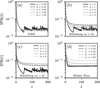
Figure 3: Evolution of the IPR for several types of networks. (a) A Newman–Watts–Strogatz (NWS) network in which each node is adjacent to its two nearest neighbors in a ring. For each edge, the probabilities of adding a new edge are $p\in\{0,0.01,0.02,0.05,1\}$. (b, c) A Kleinberg navigable small-world network with clustering exponent $\alpha$ and $q\in\{0,1,2,3,4\}$ additional connections for each node. In (b), $\alpha=2$; in (c), $\alpha=3$. (d) A Holme–Kim (HK) power-law cluster network with probability $p^{\prime}\in\{0,0.25,0.5,0.75,1\}$ of adding a triangle after adding a random edge. We construct this network by starting with an empty dyad (i.e., two isolated nodes) and iteratively adding new nodes until the network has 100 nodes. Each new node connects to two existing nodes using linear preferential attachment. All networks have $N=100$ nodes. All curves are sample means of 1000 network instantiations. We place an initial CTQW excitation at node 50.

To further study localization, we consider three additional types of networks: (i) Newman–Watts–Strogatz (NWS) small-world networks [45, 46], (ii) Kleinberg navigable small-world networks [39] with a ring structure, and (iii) Holme–Kim (HK) power-law cluster networks [40]. In the NWS network, each node is adjacent to its two nearest neighbors in a ring. For each existing edge between nodes $i$ and $j$, with probability $p$, we add a new edge between node $i$ and another node that we select uniformly at random. In the Kleinberg network, edges that one adds to the backbone ring are more likely to connect nodes that are closer to each other (with respect to distance in the ring) than those that are farther apart from each other. When adding an edge, the probability of connecting two nodes $i$ and $j$ is proportional to $d(i,j)^{-\alpha}$, where $\alpha\geq 0$ is the clustering exponent and $d(i,j)$ is the geodesic distance between nodes $i$ and $j$. (Observe that self-edges are possible.) The HK network is a generalization of the standard Barabási–Albert preferential-attachment model [47] that also adds triangles. One starts with an empty dyad (i.e., two isolated nodes). In each preferential-attachment step, one adds a new node and connects it to two existing nodes. With probability $p^{\prime}$, for each new node and new edge from the preferential-attachment step, one adds another edge and forms a triangle by connecting the new node to a neighbor of the previously linked node.

In Fig. 3, we show the IPR as a function of time for NWS, Kleinberg, and HK networks. We consider different model parameters and calculate sample means over 1000 network instantiations. For the NWS networks, we consider probabilities of $p\in\{0,0.01,0.02,0.05,1\}$ and observe that the IPR approaches values between $0.02$ and $0.03$ [see Fig. 3(a)], corresponding to a delocalized wave function. When $p=0$, the CTQW travels around the ring and interferes with itself. For the Kleinberg networks, we consider clustering exponents of $\alpha=2$ [see Fig. 3(b)] and $\alpha=3$ [see Fig. 3(c)] and we add $q$ connections per node to the underlying ring. When we do not not add any edges (i.e., $q=0$), the observed evolution of the IPR resembles that in Fig. 3(a) for $p=0$. For $\alpha=2$ and $q=1$, the IPR approaches values of about $0.05$, hinting at localization. Visual inspection of the wave-function evolution confirms that the CTQW has a noticeable amplitude for only a few nodes. As $q$ increases for the networks with $\alpha=2$, the IPRs approach smaller values than when $q=1$. For $\alpha=2$, it is likely that the edge-addition process introduces some long-range edges, causing the CTQW to propagate through the whole network rather than being confined to a local region. (This is somewhat reminiscent of the appearance of new infection clusters via long-range edges in spreading process on networks [48].) For $\alpha=3$, the added edges are more likely to connect nearby nodes than to connect distant nodes. In this case, the IPR approaches values between 0.05 and 0.06 as we increase $q$. We believe that this is due to the existence of many local clusters in the networks. In the HK networks, for $p^{\prime}$ close to 1, we observe IPR values of up to $0.1$ [see Fig. 3(d)].

Conclusions and discussion.

We examined how local clustering can induce localization in quantum walks on networks. Our work gives insights into the influence of network structure on the long-time behavior of quantum walks. We have demonstrated that local clustering can inhibit the propagation of quantum walks, which is relevant to consider when employing quantum walks in quantum communication channels [23]. Our work also suggests fascinating experimental investigations of quantum-walk localization in networks (such as with recursive triangle networks) using, e.g., photonic implementations of quantum walks [49]. In this context, it is worthwhile to study the localization effects for the potential applications of quantum walks in quantum memory, as localized quantum walks require less space than non-localized quantum walks to store and retrieve information [41].