Generative-Model-Based Fully 3D PET Image Reconstruction by Conditional Diffusion Sampling
Abstract
Score-based generative models (SGMs) have recently shown promising results for image reconstruction on simulated positron emission tomography (PET) datasets. In this work we have developed and implemented practical methodology for 3D image reconstruction with SGMs, and perform (to our knowledge) the first SGM-based reconstruction of real fully 3D PET data. We train an SGM on full-count reference brain images, and extend methodology to allow SGM-based reconstructions at very low counts (1% of original, to simulate low-dose or short-duration scanning). We then perform reconstructions for multiple independent realisations of 1% count data, allowing us to analyse the bias and variance characteristics of the method. We sample from the learned posterior distribution of the generative algorithm to calculate uncertainty images for our reconstructions. We evaluate the method’s performance on real full- and low-count PET data and compare with conventional OSEM and MAP-EM baselines, showing that our SGM-based low-count reconstructions match full-dose reconstructions more closely and in a bias-variance trade-off comparison, our SGM-reconstructed images have lower variance than existing baselines. Future work will compare to supervised deep-learned methods, with other avenues for investigation including how data conditioning affects the SGM’s posterior distribution and the algorithm’s performance with different tracers.
Index Terms:
Positron Emission Tomography, Image Reconstruction Algorithms, Deep Learning, Generative AII Introduction
Low-count positron emission tomography (PET) data arises in contexts such as low-dose administration and acquisition time reduction. However, the inverse problem of PET reconstruction from low-count data suffers from high-variance Poisson noise. Recently proposed deep learning methods incorporate learned prior information into the reconstruction process to mitigate this issue. Score-based generative models (SGMs) are state-of-the-art generative models that only require unpaired high-quality images for unsupervised training, thus decoupling scanner-specific considerations from the training process for greater generalisability [1]. State-of-the-art reconstruction has been shown for MR and CT with SGMs, while Xie et al. and Singh et al. have shown state-of-the-art simulated results for PET [7] [4]. In this work, we develop and investigate state-of-the-art SGM-based fully 3D image reconstruction methodologies on very low count real PET data, using the example of in vivo F]DPA-714 distributions.
II Theory
PET image reconstruction may be formulated as an inverse problem by modelling the mean of our measurements as
where represents the radiotracer distribution, represents our system model and models scatter and randoms components. Let be the prior probability density of image .
The SGM framework involves two stochastic processes, a forward “diffusion” process that maps from a distribution of images to a standard high-dimensional Gaussian, and its reverse, the backward process which we seek to learn. Assuming access to the score function , the backward process may be expressed analytically and numerically solved, thereby allowing us to sample from the image distribution.
We train an unconditional time-dependent SGM to model the score function from a training set of high-quality 2D transverse brain slices extracted from 3D full-count images, via denoising score matching [5].
To condition on fully 3D PET sinogram data, we alternate steps solving the backwards-time generative process with steps to encourage data consistency. One method that does this is Singh et al.’s PET-DDS, an adaptation of Decomposed Diffusion Sampling to the case of non-negative PET images with high dynamic range [4]. In PET-DDS, data consistency steps constitute gradient descent on the standard Poisson log-likelihood for subset , an axial relative difference prior (RDP) to enable 3D reconstruction and a third term to prevent straying too far from the diffusion output. As we consider reconstruction from fewer counts than Singh et al., our log-likelihood gradients are significantly larger. Therefore, we extend this algorithm to give PET-DDS-, by introducing an additional hyperparameter to moderate the rate of gradient descent () towards the reconstruction objective. Let our forward process be defined by . Let stochasticity be . Then for each of iterations, given iterate :
III Experiments
Fifty-five static F]DPA-714 brain datasets (from the Inflammatory Reaction in Schizophrenia team at King’s College London) were used for SGM training and validation [2]. Data were acquired from 1-hour scans with the Siemens Biograph mMR, with approximately 200 MBq administered, with total counts in the range . At full-count, high-quality images (voxel size 2 mm 2 mm 2 mm ; 3D image size ) were reconstructed with the scanner defaults (OSEM with 21 subsets and 2 iterations). An SGM was trained for 100 epochs (a value identified via 5-fold cross-validation) to learn the score function of these data.
An additional 7 datasets were reserved for validation and testing of the reconstruction process. For our SGM reconstruction method we used PET-DDS-, with 100 diffusion steps and 5 reconstruction objective steps per diffusion step (i.e. ). For comparison, we implemented OSEM and MAP-EM (with patch-based regularisation [6]). Each method used the same ParallelProj 3D projector [3] with span 11 axial compression applied. To obtain low-count sinograms, prompts and randoms were sampled at 1% of counts assuming independent Poisson statistics, with smoothed randoms and scatter sinograms re-estimated using scanner software.
For PET-DDS-, reconstruction hyperparameter values of , , were selected to minimise NRMSE on the validation dataset. On this dataset, reconstructions were performed on 20 independent realisations of 1% count data, allowing calculation of bias and variance. The remaining 6 datasets were used to evaluate methods at their optimal hyperparameters, with the full-count scanner reconstructions taken as ground truth.
IV Preliminary Results and Discussion
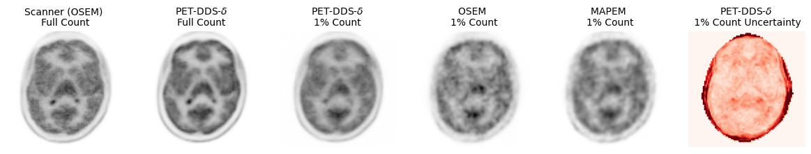
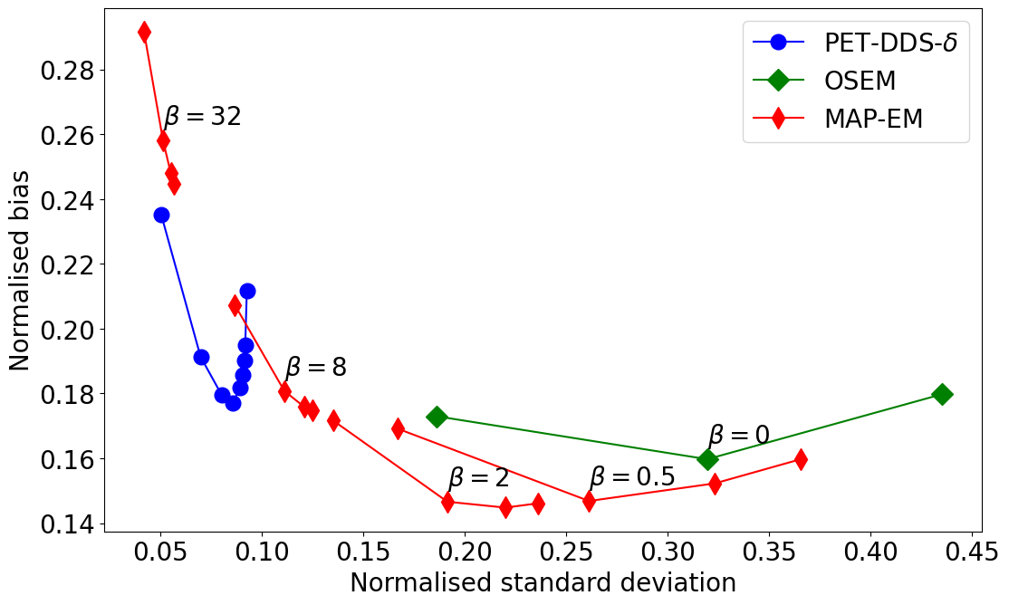
Table I shows that PET-DDS- of the 1 % data more closely matches the full-count reconstruction, achieving lower NRMSE values compared to the baseline methods as expected. This analysis is supported qualitatively by Figure 1, in which PET-DDS- retains higher visual fidelity compared to the other low-count reconstructions. In our bias-variance analysis in Figure 2, we see that the reduced NRMSE values are primarily due to reduced variance with respect to the Poisson noise realisations, with a higher minimum bias observed for PET-DDS- than for MAP-EM.
| Metric | NRMSE (%) | PSNR (dB) | SSIM (%) |
|---|---|---|---|
| OSEM | |||
| MAP-EM | |||
| PET-DDS- |
V Summary
We have developed and extended practical methodology for 3D image reconstruction from low-count PET data with SGMs, and performed SGM-based reconstruction of real fully 3D PET data. Future work will compare to other deep-learned methods, and may also focus on: investigating the relationship between the data conditioning and the SGM’s image manifold; conditioning on MR information; and, investigating the algorithm’s performance with F]FDG data.
References
- [1] Chung, H., and Ye, J. C. Score-Based Diffusion Models for Accelerated MRI. Medical Image Analysis 80 (Aug. 2022).
- [2] Muratib, F., et al. Dissection of Neuroinflammation in Schizophrenia. BJPsych Open 7, Suppl 1 (June 2021), S274–S275.
- [3] Schramm, G., and Thielemans, K. PARALLELPROJ—an Open-Source Framework for Fast Calculation of Projections in Tomography. Frontiers in Nuclear Medicine 3 (Jan. 2024).
- [4] Singh, I. R., et al. Score-Based Generative Models for PET Image Reconstruction. Machine Learning for Biomedical Imaging (Jan. 2024).
- [5] Song, Y., and Ermon, S. Generative Modeling by Estimating Gradients of the Data Distribution. In Advances in Neural Information Processing Systems (2019), vol. 32, Curran Associates, Inc.
- [6] Wang, G., and Qi, J. Penalized Likelihood PET Image Reconstruction using Patch-based Edge-preserving Regularization. IEEE transactions on medical imaging 31, 12 (Dec. 2012), 2194–2204.
- [7] Xie, T., et al. Joint Diffusion: Mutual Consistency-Driven Diffusion Model for PET-MRI Co-Reconstruction, Nov. 2023.