Quantum trails and memory effects in the phase space of chaotic quantum systems

Abstract

The eigenstates of a chaotic system can be enhanced along underlying unstable periodic orbits in so-called quantum scars, making it more likely for a particle launched along one such orbits to be found still there at long times. Unstable periodic orbits are however a negligible part of the phase space, and a question arises regarding the structure of the wavefunction elsewhere. Here, we address this question and show that a weakly-dispersing dynamics of a localized wavepacket in phase space leaves a “quantum trail” on the eigenstates, that is, makes them vary slowly when moving along a trajectories in phase space, even if not periodic. The quantum trails underpin a remarkable dynamical effect: for a system initialized in a localized wavepacket, the long-time phase-space distribution is enhanced along the short-time trajectory, which can result in ergodicity breaking. We provide the general intuition for these effects and prove them in the stadium billiard, for which an unwarping procedure allows to visualize the phase space on the two-dimensional space of the page.

Classical chaos is famously characterized by the butterfly effect, where small differences in initial conditions lead to vastly different outcomes over time [1, 2, 3]. If and how chaos manifests in quantum systems is a more nuanced question, the center of the mature field of quantum chaos [4, 5, 6, 3]. On the surface, chaotic quantum systems behave similarly to random matrices: their level statistics follows random matrix theory [7, 8, 9, 10], and their eigenstates appear rather featureless [11, 12, 13]. But, of course, physical systems are not random matrices, and deviations can occur. A striking example are quantum scars, whereby the eigenstates can show enhanced amplitude along certain classical unstable periodic orbits [14]. This enhancement means that a quantum particle is more likely to remain localized along an orbit it was prepared on, which can lead to a form of ergodicity breaking [15]. More recently, these phenomena have been shown to play an important role in our understanding of isolated many-body systems out of equilibrium [16, 17, 18, 19, 20, 21, 22, 23], as increasingly relevant in modern quantum simulators [24, 25, 26].

Yet, unstable periodic orbits occupy only an infinitesimally small fraction of the phase space, raising a natural question: how does the quantum wavefunction behave in the vast regions of phase space that are not tied to these special orbits?

Here, we address this question and find that, if a wavepacket moves along a trajectory with little dispersion, then a “quantum trail” is left on the eigenstates, namely the projection of the eigenstates in phase space varies slowly along the trajectory. As a direct consequence of quantum trails, an initially localized wavepacket fails to uniformly scramble across the accessible phase space: the long-time distribution is enhanced along the short-time trajectory, a memory effect that can break ergodicity. We illustrate these concepts in the paradigmatic stadium billiard, for which a phase-space unwarping procedure facilitates the visualization of the trails. Our work unveils the structure of the eigenstates in phase space, shows its implications on the long-time dynamics, and contributes to our understanding of the classical-quantum correspondence.

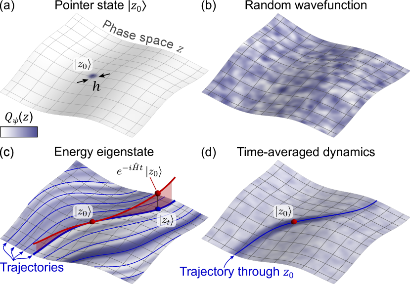
Figure 1: Quantum states in phase space: trails and memory effects. Schematic projections $Q_{\psi}(z)$ on a phase space of coordinates $z$. (a) A pointer state $\ket{z_{0}}$ is localized around $z_{0}$ over some length $\sim h$. (b) A random wavefunction yields a speckled pattern with features of size $\sim h$. (c) An eigenstate $\ket{E}$ can yield quantum trails, that is, speckles of width $\sim h$ and length $>h$ that elongate along the trajectories $z_{t}$ (blue lines). The trails extend as long as $\ket{z_{t}}\approx e^{-i\hat{H}t}\ket{z_{0}}$. (d) Due to the trails, a system initialized in $\ket{z_{0}}$ is, at long times, more likely to be found on the short-time trajectory through $z_{0}$, a memory effect that can break ergodicity.

General intuition and phenomenology—Consider a quantum system with Hamiltonian $\hat{H}$ and a phase space of coordinates $z=(z_{1},z_{2},\dots)$. Denote $\ket{z}$ a pointer state localized around the point $z$ of the phase space, Fig. 1(a), and say $h$ the characteristic localization length. The projection of a wavefunction $\ket{\psi}$ on phase space reads $Q_{\psi}(z)=\left|\langle z|\psi\rangle\right|^{2}$, and that of a random (e.g., Haar random) state $\ket{\psi_{\rm rand}}$ appears as a chaotic speckled pattern with correlation length $\sim h$, Fig. 1(b).

The eigenstates $\ket{E}$ can be strikingly different. The key point is: if the pointer state $\ket{z_{t}}$ associated to a trajectory $z_{t}$ in phase space is close to the actual dynamics from $\ket{z_{0}}$, namely if $e^{-i\hat{H}t}\ket{z_{0}}\approx\ket{z_{t}}$, then it immediately follows that $\langle E|z_{t}\rangle\approx e^{-iEt}\langle E|z_{0}\rangle$ and $Q_{E}(z_{t})\approx Q_{E}(z_{0})$, even if $|z_{t}-z_{0}|\gg h$. In other words, if wavepackets in phase space evolve without immediately dispersing, $e^{-i\hat{H}t}\ket{z_{0}}\approx\ket{z_{t}}$, then the eigenstates in phase space cannot consist of a speckled pattern as in Fig. 1(b), but must instead consist of elongated speckles, or “quantum trails”, as in Fig. 1(c). The trails imply a rich correlation structure in phase space: while the projections $Q_{E}(z_{0})$ and $Q_{E}(z_{t})$ can behave like pseudo-random numbers (e.g., with Porter-Thomas distribution [27, 28]), they will be correlated with each other if $z_{t}$ is on the short-time trajectory through $z_{0}$. The “short-time trajectory” is the segment of trajectory for which the condition $\ket{z_{t}}\approx e^{-i\hat{H}t}\ket{z_{0}}$ still holds. Its length determines that of the trails and of the correlations in $Q_{E}(z)$. In contrast to scars [15], the trails do not require unstable periodic orbits nor localization.

The structure of the eigenstates has direct and dramatic effects on the dynamics. The question we ask is: starting from $\ket{z_{0}}$, where does the system end up at long times, on average? This is quantified by the time-averaged phase-space projection [29, 30, 31, 32, 21]

$$\bar{Q}(z|z_{0}) =\lim\limits_{T\to\infty}\frac{1}{T}\int_{0}^{T}dt\ \left|\langle z|e^{-i\hat{H}t}|z_{0}\rangle\right|^{2},$$ (1)

$$=\sum_{E}Q_{E}(z_{0})Q_{E}(z),$$ (2)

which we expanded in the energy basis assuming a non-degenerate spectrum. For an eigenstate $\ket{E}$ to significantly contribute to the sum, both $Q_{E}(z_{0})$ and $Q_{E}(z)$ should be relatively large, that is, the initial condition $\ket{z_{0}}$ should have a significant component over the eigenstate and the eigenstate should matter for the observation point $z$. A correlation between $Q_{E}(z_{0})$ and $Q_{E}(z)$ means that, if one condition is met, the other is met “for free”, thus enhancing $\bar{Q}(z|z_{0})$. The extreme case is $z=z_{0}$, for which the correlation is perfect and the enhancement of $\bar{Q}(z_{0}|z_{0})$ known [31, 32].

Crucially, the quantum trails in the eigenstates imply that the correlation between $Q_{E}(z_{0})$ and $Q_{E}(z)$ stretches along the short-time trajectory $z_{t}$ through $z_{0}$, in turn implying an enhanced time-averaged projection $\bar{Q}$ there, see Fig. 1(d). One could say that quantum mechanics leaves no second chances: if at short-times the system does not quickly disperse in phase space, it never fully will. The effect is particularly remarkable if the underlying trajectories are ergodic: a classical ensemble fills the phase space uniformly at long times, but a quantum wavepacket does not, retaining information on the initial condition and thus breaking ergodicity [31]. Under standard assumptions for chaotic quantum systems, in Appendix A we estimate the contrast of the enhancement in $\bar{Q}$, namely the ratio between $\bar{Q}(z_{t}|z_{0})$ on a point $z_{t}$ of the trajectory through $z_{0}$ and $\bar{Q}(z_{g}|z_{0})$ on a generic point $z_{g}$ of the accessible phase space,

$$\frac{\bar{Q}(z_{t}|z_{0})}{\bar{Q}(z_{g}|z_{0})}\approx 1+\left|\langle z_{t}|e^{-i\hat{H}t}|z_{0}\rangle\right|^{2}.$$ (3)

The contrast is $\approx 2$ when $\ket{z_{t}}\approx e^{-i\hat{H}t}\ket{z_{0}}$, suggesting that in the classical limit $h\to 0$ the enhancement in $\bar{Q}$ becomes infinitesimally narrow but does not loose contrast, and recovering the doubled return probability in the limit case of $t=0$ [32].

The treatment was so far general and prioritized conceptual clarity over technical precision. We have deliberately kept the notion of phase space $z$, trajectories $z_{t}$, and pointer states $\ket{z}$ vague. Their choice is indeed ultimately arbitrary and problem-dependent. For a semiclassical system, $z$ and $z_{t}$ can be naturally taken from the classical limit. For a many-body system, $z$ could be the parameters of a variational wavefunction $\ket{z}$, and the trajectories $z_{t}$ given by the time-dependent variational principle (TDVP) [33, 34, 35, 36]. In the end, the key condition for the quantum trails is that $\ket{z_{t}}$ is for some time a good approximation of the actual dynamics, namely that $\left|\langle z_{t}|e^{-i\hat{H}t}|z_{0}\rangle\right|^{2}\sim 1$, and this should drive the choice of $z$, $z_{t}$, and $\ket{z}$ for a given $\hat{H}$.

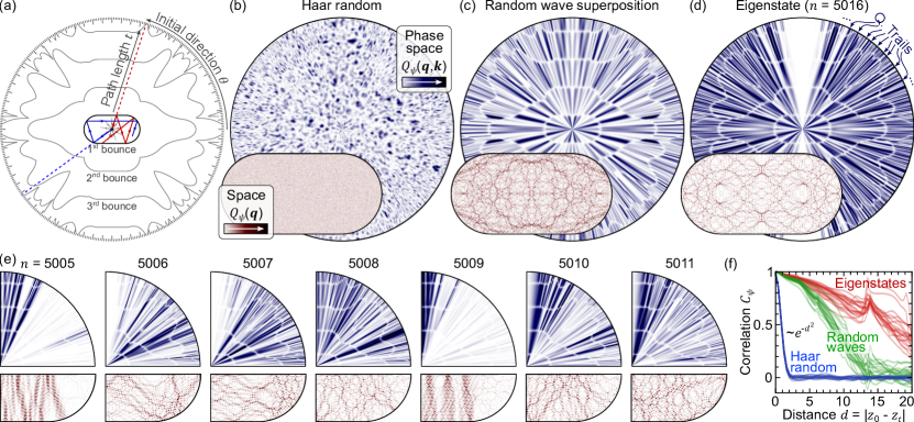
Figure 2: Quantum trails in a chaotic billiard. (a) An unwarping technique allows to represent the three-dimensional phase space on the two dimensional page, as follows. Consider a trajectory $(\bm{q}_{t},\bm{k}_{t})_{\theta}$ (solid red) from $\bm{q}_{0}=(0,0)$ and $\bm{k}_{0}=k(\cos\theta,\sin\theta)$. We associate the points $\bm{q}=\bm{k}_{0}t$ of the page (red dashed line) to the points $(\bm{q}_{t},\bm{k}_{t})_{\theta}$ of the phase space. The polar coordinates $t$ and $\theta$ on the page can be used to move in phase space along the trajectories and away from them, respectively. (b) A Haar random state yields a speckled pattern in phase space (blue), and a collection of random pixels in space (red). (c) A random wave superposition yields, in phase space, partial trails that extend along trajectories but are interrupted by the collisions with the boundary of the billiard. (d) An eigenstate $\ket{k_{n}}$ is similar to a random wave superposition in space, but strickingly different in phase space: full-fledged quantum trails stretch along the trajectories (radially on the page), even across collisions with the boundary. (e) Projection of consecutive eigenstates $\ket{k_{n}}$. Some eigenstates are scarred, namely localized along unstable periodic orbits (e.g., $n=5005$ and $5009$). The quantum trails are a more general feature: the eigenstates (both scarred and not) correlate along the trajectories (both periodic and not). (f) Pearson correlation coefficient between $Q_{\psi}(z_{0})$ and $Q_{\psi}(z_{t})$ versus distance $d=|z_{0}-z_{t}|$, computed sampling points $z_{0}$ uniformly in phase space and points $z_{t}$ along the short-time ($t<3/\lambda\approx 3.49/k$) dynamics from $z_{0}$. For Haar random states (blue), the correlation trivially decays as $\sim e^{-d^{2}}$. For the random wave superpositions (green), but even more for the eigenstates (from $n=5009$ to $n=5028$, red), the correlation extends over large distances $d$, due to the quantum trails. Here, $k=94.68$.

The stadium billiard—We prove these ideas in a paradigmatic model of quantum chaos: the stadium billiard [37, 38]. This consists of a particle in a box, $\hat{H}=\frac{\bm{\hat{p}}^{2}}{2m}+V(\hat{\bm{q}})$, with $V(\bm{q})=0$ inside the billiard and $V(\bm{q})=\infty$ outside of it. We set $m=\hbar=1$ and consider the billiard of height $2R=2$ and width $2R+L=4$. We use the boundary integral method to numerically find the spectrum $\hat{H}\ket{k_{n}}=\frac{k_{n}^{2}}{2}\ket{k_{n}}$ [39, 40].

The phase space consists of position $\bm{q}=(q_{x},q_{y})$ and momentum $\bm{k}=(k_{x},k_{y})$. The trajectories $z_{t}$ are the classical ones and the momentum $\bm{k}=k(\cos\theta,\sin\theta)$ has conserved $|\bm{k}|=k$, so that the phase space can be reduced to three dimensions, $z=(q_{x},q_{y},\theta)$. As pointer states $\ket{\bm{q}\bm{k}}$ we consider Gaussian wavepackets with centroid $(\bm{q},\bm{k})$, which in the position basis read $\langle\bm{q}^{\prime}|\bm{q}\bm{k}\rangle=\frac{1}{\sigma\sqrt{\pi}}e^{-\frac{|\bm{q}-\bm{q}^{\prime}|}{2\sigma^{2}}+i\bm{q}^{\prime}\cdot\bm{k}}$ [41, 32, 42]. The respective uncertainties $\langle(\Delta q_{x,y})^{2}\rangle=\frac{\sigma^{2}}{2}$ and $\langle(\Delta k_{x,y})^{2}\rangle=\frac{1}{2\sigma^{2}}$ saturate the Heisenberg uncertainty principle, and to ensure a similar localization in position and momentum we enforce $\frac{\langle(\Delta q_{x,y})^{2}\rangle}{R^{2}}=\frac{\langle(\Delta k_{x,y})^{2}\rangle}{k^{2}}\ll 1$, that is, set $\sigma^{2}=\frac{1}{k}$ and work in the semiclassical regime $k\gg 1$ [40].

A wavefunction $\ket{\psi}$ can be visualized using either the space projection $Q_{\psi}(\bm{q})=\left|\langle\bm{q}|\psi\rangle\right|^{2}$ or the phase-space projection $Q_{\psi}(\bm{q}\bm{k})=\left|\langle\bm{q}\bm{k}|\psi\rangle\right|^{2}$. The former is the standard probability density in space and allows to view scars [14], whereas the latter corresponds to $Q_{\psi}(z)$ in our general formalism above and allows to view the quantum trails. Visualization in phase space is in fact nontrivial, due to its dimensionality $>2$. Previous work has focused on a Poincaré section by rewriting the dynamics $z_{t}$ as a map between Birkhoff coordinates at consecutive bounces [43, 44, 45, 46, 47]. This technique however does not allow a clear visualization of the quantum trails, because the trajectories appear in the Poincaré section as sequences of disconnected points, breaking the trails into pieces [48, 49]. We therefore devise an alternative strategy to represent the three-dimensional phase space on the two-dimensional page.

The task of scanning the phase space can in fact be effectively delegated to the trajectories: due to ergodicity [37, 38], even a single “probe” trajectory $(\bm{q}_{t},\bm{k}_{t})$ will at $t\to\infty$ explore the whole phase space (excluding the measure-0 set of periodic orbits). That is, the finite three-dimensional phase space of coordinates $z=(q_{x},q_{y},\theta)$ can be “unwarped” onto an infinite one-dimensional space of parametric coordinate $t$, allowing to inspect how the projection $Q_{\psi}(\bm{q}_{t}\bm{k}_{t})$ varies along a trajectory. To fully appreciate a quantum trail, however, we also need to inspect the phase space in a direction orthogonal to $z_{t}$. Thus, instead of launching a single probe trajectory we launch a fan of them, $(\bm{q}_{t},\bm{k}_{t})_{\theta}$, starting from the middle of the billiard with direction $\theta$ varying continuously in $[0,2\pi]$, see gray lines in the middle of Fig. 2(a). A point of the page with polar coordinates $\theta$ and $t$ will then correspond to a point of the phase space $(\bm{q}_{t},\bm{k}_{t})_{\theta}$. Varying $t$ and $\theta$ allows to move along trajectories or away from them, respectively. In this representation, the quantum trails correspond to features that stretch radially on the page.

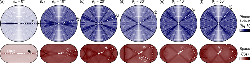
Figure 3: Memory effect and ergodicity breaking in a chaotic billiard. We solve the dynamics $e^{-i\hat{H}t}\ket{\bm{q}_{0}\bm{k}_{0}}$ from a wavepacket $\ket{\bm{q}_{0}\bm{k}_{0}}$ launched from the middle of the billiard with various angles $\theta_{0}$ and compute the time-averaged projection $\bar{Q}$ both in space and in phase space. The quantum trails in the eigenstates result in an enhancement of $\bar{Q}$ along the short-time trajectory through $(\bm{q}_{0},\bm{k}_{0})$ (dashed white line). The system thus retains a memory of its initial condition and breaks ergodicity. In real space, the enhancement of $\bar{Q}(\bm{q})$ is particularly evident in the form of “caustics” on the short-time trajectories (see [40] for enlarged figures). For wavepackets launched along unstable periodic orbits (UPOs, for $\theta=0^{\circ},30^{\circ}$) the effect appears slightly stronger, which can be explained by quantum scars. Here, $k=148.80$.

We begin by considering in Fig. 2(b) a Haar random state . The space projection $Q_{\rm Haar}(\bm{q})$ is a collection of random pixels, and the phase-space projection $Q_{\rm Haar}(\bm{q}\bm{k})$ exhibits a speckled pattern analogous to that predicted in Fig. 1(a). A closer analogue of the eigenstates is a random wave superposition with momentum $k$ [11], namely $\langle\bm{q}|\psi_{\rm rw}\rangle\sim\sum_{n=1}^{N}e^{i(\bm{k}_{n}\cdot\bm{q}+\phi_{n})}$ (see  for details). In space, $Q_{\rm rw}(\bm{q})$ consists of a pattern with spatial features of size $\sim\frac{2\pi}{k}$, see Fig. 2(c). In phase space, $Q_{\rm rw}(\bm{q}\bm{k})$ is approximately uniform when moving along a trajectory, but only until the next collision with the boundary of the billiard, creating a partial quantum trail. This is understood by considering three points $z,z^{\prime}$, and $z^{\prime\prime}$ on a trajectory, with no boundary collision separating $z$ and $z^{\prime}$ and with one boundary collision separating $z^{\prime}$ and $z^{\prime\prime}$, namely, $\bm{k}=\bm{k^{\prime}}\neq\bm{k}^{\prime\prime}$. The wave components that most contribute to $Q_{\rm rw}(z)$ and $Q_{\rm rw}(z^{\prime})$ are the same, namely those with $\bm{k}_{n}\approx\bm{k}=\bm{k}^{\prime}$, whereas the wave components that matter for $Q_{\rm rw}(z^{\prime\prime})$ are different, namely those with $\bm{k}_{n}\approx\bm{k}^{\prime\prime}$. That is, a trail connects $z$ and $z^{\prime}$, but not $z^{\prime}$ and $z^{\prime\prime}$.

Finally, in Fig. 2(d) we consider the most interesting case of an energy eigenstate $\ket{k_{n}}$. The space projection $Q_{k_{n}}(\bm{q})$ is qualitatively similar to that of a random wave superposition [11]. The phase-space projection $Q_{k_{n}}(\bm{q}\bm{k})$ is markedly different: it correlates radially along the trajectories, even when these go through collisions with the boundary of the billiard. That is, for the eigenstates we find and visualize full-fledged quantum trails. This is not contingent on the specific choice of the eigenstate: in Fig. 2(e) we show the quantum trails in $7$ consecutive eigenstates. The symmetries of the problem allow us to focus on just one quarter of the phase space. Some eigenstates appear clearly scarred, namely localized along unstable periodic orbits (e.g., for $n=5005$ and $5009$). Other eigenstates are not visibly scarred, and yet they exhibit quantum trails across the whole phase space (e.g., for $n=5008,5011$, and $5016$).

A quantitative analysis is provided in Fig. 2(f) by computing the Pearson correlation coefficient $C_{\psi}$ between $Q_{\psi}(z_{0})$ and $Q_{\psi}(z_{t})$ for a fixed $\ket{\psi}$ and with respect to an ensemble of pairs $(z_{0},z_{t})$. The latter are obtained sampling $z_{0}$ uniformly in phase space, and $z_{t}$ uniformly along the short-time trajectory from $z_{0}$, that is, sampling $t$ uniformly from $[0,\frac{3}{\lambda}]$, with $\lambda\approx 0.86k$ the numerically computed Lyapunov exponent. The correlation $C_{\psi}$ is plotted versus the phase-space distance $d=|z_{0}-z_{t}|$, which we naturally define as $d^{2}\mathrel{\mathop{:}}=-\log(\left|\langle z_{0}|z_{t}\rangle\right|^{2})=\frac{k}{2}\left(|\bm{q}_{0}-\bm{q}_{t}|^{2}+\frac{|\bm{k}_{0}-\bm{k}_{t}|^{2}}{k^{2}}\right)$. For the Haar random state, the correlation $C_{\psi}$ trivially relies on an overlap between $\ket{z_{0}}$ and $\ket{z_{t}}$, and thus quickly decays as $C_{\psi}\sim e^{-d^{2}}$. A longer correlation is found for the random wave superpositions, thanks to their partial trails. But it is the eigenstates that, thanks to their full-fledged trails, yield the strongest and longest correlations.

Next, to see the memory effects that the quantum trails underpin, we launch a wavepacket with position $\bm{q}_{0}=(0,0)$ and momentum $\bm{k}_{0}=k(\cos\theta_{0},\sin\theta_{0})$ and inquire about its time-averaged projection in Eq. (2), namely $\bar{Q}(\bm{q}\bm{k})=\sum_{E}Q_{E}(\bm{q}\bm{k})Q_{E}(\bm{q}_{0}\bm{k}_{0})$, shown in Fig. 3 for various initial directions $\theta_{0}$. The classical billiard is ergodic [37, 38], which suggests a uniform $\bar{Q}$ irrespective of $\theta_{0}$. By striking contrast, the quantum trails in the eigenstates imply that $\bar{Q}$ is enhanced along the short-time trajectory from $(\bm{q}_{0},\bm{k}_{0})$, which depends on $\theta_{0}$: the system retains memory of the initial condition and ergodicity is broken.

Our intuition was built in phase space, but the effects persist in real space. To see this we modify the time-averaged phase-space projection in Eq. (2) into a time-averaged space projection [31], $\bar{Q}(\bm{q})=\sum_{E}\left|\langle\bm{q}|E\rangle\right|^{2}Q_{E}(\bm{q}_{0}\bm{k}_{0})$, that is nothing but the probability density of finding the particle in position $\bm{q}$ at a random time $t\ggg 1$. Loosely speaking, we can think of $\bar{Q}(\bm{q})$ as obtained integrating out the momentum from $\bar{Q}(\bm{q}\bm{k})$, which can reduce the memory effect without suppressing it. Indeed, in the bottom of Fig. (3) we observe that $\bar{Q}(\bm{q})$ is enhanced along the short-time orbit, particularly in the form of caustics. The contrast of the enhancement in $\bar{Q}$ appears slightly larger when the system is launched along an unstable periodic orbit, namely for $\theta_{0}=0^{\circ}$ and $30^{\circ}$ in Fig. 3, which can be explained by quantum scarring. Our key finding is that the ergodicity is broken more in general, due to quantum trails, even for trajectories that are not on unstable periodic orbits. Note that $\left|\langle\bm{q}|E\rangle\right|^{2}$ is invariant upon horizontal or vertical mirroring, and so is $\bar{Q}(\bm{q})$. Enlarged figures for $\bar{Q}(\bm{q})$ are shown in [40].

In conclusion, we have unveiled the structure of chaotic eigenstates in phase space and the memory effects that it implies. The core intuition for quantum scars is that if a wavepacket goes around an unstable periodic orbit with limited dispersion, then some eigenstates will be localized along the orbit and a system initialized on it is more likely to remain there [15]. Quantum trails modify and extend this intuition to all the trajectories, even non-periodic ones: if the wavepacket follows a trajectory $z_{t}$ with limited dispersion, meaning $e^{-i\hat{H}t}\ket{z_{0}}\approx\ket{z_{t}}$, then quantum trails are left in the eigenstates, and a system initialized in $\ket{z_{0}}$ has an enhanced probability of being found on the short-time trajectory through $z_{0}$, even at long times. In quantum scars, like in semiclassical localization [41], Anderson localization [52], and many-body localization [53, 54], the memory effect can be attributed to the localization of the eigenstates. Crucially, we have shown that eigenstate localization is in fact not necessary for a memory effect: correlations of the eigenstates along the trajectories, i.e., quantum trails, suffice. The condition for this, namely that an initially localized wavepacket should not immediately disperse in phase space, is a generous one, suggesting that trails and memory effects should be recurring features of quantum systems, both chaotic and non, opening the way to much further research. Beyond assessing these effects in other single-particle systems, such as dispersing billiards, softened billiards, and quantum maps, a particularly timely question regards the implications of quantum trails on many-body quantum systems, in particular with respect to thermalization, ergodicity, and entanglement.

Note added: While completing this paper, the author became aware through discussions with Prof. E. Heller and his group of closely related work that then appeared in Ref. [55], in which the memory effects in Fig. 3 are dubbed “birthmarks” and both the stadium billiard and block-random matrix models are studied.

Acknowledgements. The author acknowledges support by Trinity College Cambridge and discussions related to this work with A. Buchleitner, C. B. Dag, B. Evrard, E. Heller, W. W. Ho, J. Knolle, A. Lamacraft, M. McGinley, and L. Sá.

I Appendix A

In this Appendix we estimate the contrast of the trail in the time-averaged projection $\bar{Q}$, namely Eq. (3).

Consider a binning of the energy, and say $\mathcal{E}_{n}$ the set of eigenvalues $E$ in the $n$-th bin, namely with $n\epsilon\leq E<(n+1)\epsilon$, with $\epsilon$ the bin width. Consider that the bin width can be taken large compared to the mean energy spacing, but small compared to the involved energy scales (e.g., $\langle z|\hat{H}|z\rangle$), which is possible for semiclassical and many-body quantum chaotic systems. Let us denote $\langle\dots\rangle_{n}=\mathcal{N}_{n}^{-1}\sum_{E\in\mathcal{E}_{n}}(\dots)$ the average over the $n$-th bin, with $\mathcal{N}_{n}\gg 1$ the number of eigenvalues in it. The sum over the energies can be written as a sum over bins, namely $\sum_{E}(\dots)=\sum_{n}\mathcal{N}_{n}\langle\dots\rangle_{n}$, and so

$$\bar{Q}(z|z_{0})=\sum_{n} \mathcal{N}_{n}\langle Q_{E}(z)Q_{E}(z_{0})\rangle_{n},$$ (4)

$$=\sum_{n} \mathcal{N}_{n}\big{[}\langle Q_{E}(z)\rangle_{n}\langle Q_{E}(z_{0})\rangle_{n}+\dots$$

$$\text{cov}_{n}\left(Q_{E}(z),Q_{E}(z_{0})\right)\big{]},$$ (5)

$$=\sum_{n} \mathcal{N}_{n}\langle Q_{E}(z)\rangle_{n}\langle Q_{E}(z_{0})\rangle_{n}\times\dots$$

$$\left[1+\text{cov}_{n}\left(\frac{Q_{E}(z)}{\langle Q_{E}(z)\rangle_{n}},\frac{Q_{E}(z_{0})}{\langle Q_{E}(z_{0})\rangle_{n}}\right)\right],$$ (6)

where $\text{cov}_{n}$ denotes the covariance computed with respect to the ensemble of eigenvalues $E\in\mathcal{E}_{n}$. Let us assume that $\langle\bar{Q}_{E}^{2}(z)\rangle_{n}\approx 2\langle\bar{Q}_{E}(z)\rangle_{n}^{2}$. This assumption is verified, e.g., if the normalized projections $\frac{\bar{Q}_{E}(z)}{\langle\bar{Q}_{E}(z)\rangle_{n}}$ have a Porter-Thomas (that is, exponential) distribution for $E\in\mathcal{E}_{n}$, which is a general universal feature of quantum chaotic systems [27, 28]. Under this assumption, the variance of $\frac{\bar{Q}_{E}(z)}{\langle\bar{Q}_{E}(z)\rangle_{n}}$ is $1$, and the covariance can be replaced by a Pearson correlation coefficient $\text{corr}_{n}$, which has the advantage of taking the simple values $0$ and $1$ for uncorrelated and perfectly correlated variables, respectively. Because the Pearson correlation coefficient is invariant under scaling of its arguments, we can lift the denominators and get

$$\bar{Q}(z|z_{0})\approx\sum_{n} \mathcal{N}_{n}\langle Q_{E}(z)\rangle_{n}\langle Q_{E}(z_{0})\rangle_{n}\times\dots$$

$$\left[1+\text{corr}_{n}\left(Q_{E}(z),Q_{E}(z_{0})\right)\right].$$ (7)

For a generic phase-space point $z_{g}$ not on the short-time trajectory from $z_{0}$, we have $\text{corr}_{n}\left(Q_{E}(z_{g}),Q_{E}(z_{0})\right)\approx 0$. Instead, the quantum trails in the eigenstates mean that for a point $z_{t}$ on the short-time dynamics through $z_{0}$ the projections $Q_{E}(z_{t})$ and $Q_{E}(z_{0})$ are correlated, to an extent which we now estimate.

The pointer state $\ket{z_{t}}$ fails to exactly follow the true dynamics $e^{-i\hat{H}t}\ket{z_{0}}$. We can thus write $\ket{z_{t}}=\sqrt{\alpha}e^{-i\hat{H}t}\ket{z_{0}}+\sqrt{1-\alpha}\ket{r_{t}}$, with $\ket{r_{t}}$ a state orthogonal to $e^{-i\hat{H}t}\ket{z_{0}}$ and $\alpha=\left|\langle z_{t}|e^{-i\hat{H}t}|z_{0}\rangle\right|^{2}$. We have

$$Q_{E}(z_{t})=\left|\langle E|z_{t}\rangle\right|^{2}=\left|\sqrt{\alpha}e^{iEt}\langle E|z_{0}\rangle+\sqrt{1-\alpha}\langle E|r_{t}\rangle\right|^{2}.$$ (8)

The state $\ket{r_{t}}$ by construction contains the bits of the wavepacket $e^{-i\hat{H}t}\ket{z_{0}}$ that get dispersed beyond $\ket{z_{t}}$, and it is thus sensible to assume that $\langle E|z_{0}\rangle$ and $\langle E|r_{t}\rangle$ are statistically independent. Moreover, if the eigenstates in $\mathcal{E}_{n}$ are similarly spread across phase space due to chaos, then we can assume that $\langle Q_{E}(z)\rangle_{n}\approx\langle Q_{E}(z_{0})\rangle_{n}$ for all the phase space points of interest $z$. Under these assumptions, from Eq. 8 we compute $\text{corr}_{n}\left(Q_{E}(z_{t}),Q_{E}(z_{0})\right)\approx\alpha$, and thus get

$$\bar{Q}(z_{t}|z_{0}) \approx\left[1+\left|\langle z_{t}|e^{-i\hat{H}t}|z_{0}\rangle\right|^{2}\right]\sum_{n}\mathcal{N}_{n}\langle Q_{E}(z_{0})\rangle_{n}^{2},$$ (9)

$$\bar{Q}(z_{g}|z_{0}) \approx\sum_{n}\mathcal{N}_{n}\langle Q_{E}(z_{0})\rangle_{n}^{2}.$$ (10)

The contrast in the trail of the time averaged projection $\bar{Q}(z|z_{0})$ thus yields

$$\frac{\bar{Q}(z_{t}|z_{0})}{\bar{Q}(z_{g}|z_{0})}\approx 1+\left|\langle z_{t}|e^{-i\hat{H}t}|z_{0}\rangle\right|^{2}.$$ (11)

Supplementary Material for
“Quantum trails and memory effects in the phase space of chaotic quantum systems”
Andrea Pizzi

This Supplementary Material is devoted to a few details on the stadium billiard. In Section I we elaborate on the methods for the numerics, and in Section II we provide high resolution zooms of the time-averaged wavefunction projection $\bar{Q}(\bm{q})$.

II I - Details on numerics

We solve the eigenvalue problem for the stadium billiard using the boundary integral method and following closely Ref. [39]. This method recasts the eigenproblem $\hat{H}\ket{k_{n}}=\frac{k_{n}^{2}}{2}\ket{k_{n}}$ to one on the boundary of the billiard. For a billiard with radius $R=1$ and width equal to twice the height, the total perimeter is $\mathcal{L}=2\pi+4$. The space discretization step is $\Delta=\frac{\mathcal{L}}{M}$, where $M$ is the number of boundary discretization points. The discretization $\Delta$ sets an upper bound to the eigenvalues $k_{n}$ that we can resolve: we again follow Ref. [39] and set $k_{\rm max}=\frac{2\pi}{10\Delta}$. We say $N$ the number of eigenstates with $k_{n}<k_{\rm max}$.

A wavepacket $\ket{\bm{q}\bm{k}}$ has position standard deviation $\frac{\sigma}{\sqrt{2}}$ and momentum standard deviation $\frac{1}{\sqrt{2}\sigma}$, where $\sigma=\sigma(k)=\frac{1}{\sqrt{k}}$ is chosen to guarantee a good localization in phase space (see main text). For a wavepacket to be well-represented in terms of the numerically available eigenstates, we require that up to 4 standard deviations of the wavepacket should be within the resolved $k_{\rm max}$, that is, that $k+\frac{4}{\sqrt{2}\sigma(k)}<k_{\rm max}$. This condition can be massaged into $k<(\sqrt{k_{\rm max}+2}-\sqrt{2})^{2}$. In the main text, we consider $M=2000$ in Fig. 2, for which $N=8386$, $k_{\rm max}\approx 122$, $k\approx 94.67$, and $\sigma\approx 0.103$, and $M=3000$ in Fig. 3, for which $N=18946$, $k_{\rm max}\approx 183.30$, $k\approx 148.80$, and $\sigma\approx 0.082$. In Fig. 2 we consider the eigenstates with $k_{n}\approx k$, namely $k_{5005}\approx 94.544$, $k_{5006}\approx 94.552$, $k_{5007}\approx 94.583$, $k_{5008}\approx 94.593$, $k_{5009}\approx 94.599$, $k_{5010}\approx 94.603$, $k_{5011}\approx 94.639$, $k_{5016}\approx 94.660$.

III II - High resolution time averaged projections

In Fig. S1 we report the same plots of $\bar{Q}(\bm{q})=\sum_{E}\left|\langle\bm{q}|E\rangle\right|^{2}Q_{E}(\bm{q}_{0}\bm{k}_{0})$ as in Fig. 2 in the main text, but enlarged to improve visibility. Moreover, because all eigenstates are either symmetric or anti-symmetric upon vertical and horizontal reflections, the projection $\left|\langle\bm{q}|E\rangle\right|^{2}$ is symmetric with respect to such reflections, and so is the time-averaged projection $\bar{Q}(\bm{q})$. In order to understand the structure in $\bar{Q}(\bm{q})$, it is thus sensible to overlap not only the classical short-time trajectories starting from $(\bm{q}_{0}\bm{k}_{0})$, but also its three mirrored versions obtained upon horizontal reflection, vertical reflection, or both. This allows to fully appreciate how much of the structure of $\bar{Q}(\bm{q})$, and in particular its caustics, can be predicted from the short-time classical trajectories.

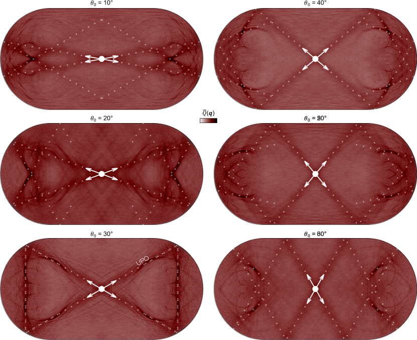
Fig. S1: Details of the time-averaged projection. We report the results for $\bar{Q}(\bm{q})$ from Fig. 2 in the main text, but with larger resolution and overlapping not just the short-time classical trajectory, but also its mirrored copies. The long-time projection of the wavefunction is enhanced along the short-time classical trajectory. It can be fully appreciated that the caustics of $\bar{Q}(\bm{q})$ tend to lie on the short-time trajectories, that depend on the initial angle $\theta_{0}$.

References

- Lorenz [1963] E. N. Lorenz, Deterministic nonperiodic flow, Journal of atmospheric sciences 20, 130 (1963).
- Strogatz [2018] S. H. Strogatz, Nonlinear dynamics and chaos: with applications to physics, biology, chemistry, and engineering (CRC press, 2018).
- Wimberger [2014] S. Wimberger, Nonlinear dynamics and quantum chaos, Vol. 10 (Springer, 2014).
- Berry [1989] M. Berry, Quantum chaology, not quantum chaos, Physica Scripta 40, 335 (1989).
- Jensen [1992] R. V. Jensen, Quantum chaos, Nature 355, 311 (1992).
- Delande and Buchleitner [1994] D. Delande and A. Buchleitner, Classical and quantum chaos in atomic systems, in Advances in atomic, molecular, and optical physics, Vol. 34 (Elsevier, 1994) pp. 85–123.
- Bohigas et al. [1984] O. Bohigas, M.-J. Giannoni, and C. Schmit, Characterization of chaotic quantum spectra and universality of level fluctuation laws, Physical review letters 52, 1 (1984).
- Berry [1987] M. V. Berry, Quantum chaology (the bakerian lecture), in A Half-Century of Physical Asymptotics and Other Diversions: Selected Works by Michael Berry (World Scientific, 1987) pp. 307–322.
- Atas et al. [2013] Y. Y. Atas, E. Bogomolny, O. Giraud, and G. Roux, Distribution of the ratio of consecutive level spacings in random matrix ensembles, Physical review letters 110, 084101 (2013).
- Kos et al. [2018] P. Kos, M. Ljubotina, and T. Prosen, Many-body quantum chaos: Analytic connection to random matrix theory, Physical Review X 8, 021062 (2018).
- Berry [1977] M. V. Berry, Regular and irregular semiclassical wavefunctions, Journal of Physics A: Mathematical and General 10, 2083 (1977).
- Hortikar and Srednicki [1998] S. Hortikar and M. Srednicki, Correlations in chaotic eigenfunctions at large separation, Physical review letters 80, 1646 (1998).
- Rigol et al. [2008] M. Rigol, V. Dunjko, and M. Olshanii, Thermalization and its mechanism for generic isolated quantum systems, Nature 452, 854 (2008).
- Heller [1984] E. J. Heller, Bound-state eigenfunctions of classically chaotic hamiltonian systems: scars of periodic orbits, Physical Review Letters 53, 1515 (1984).
- Kaplan and Heller [1998] L. Kaplan and E. Heller, Linear and nonlinear theory of eigenfunction scars, Annals of Physics 264, 171 (1998).
- Turner et al. [2018] C. J. Turner, A. A. Michailidis, D. A. Abanin, M. Serbyn, and Z. Papić, Weak ergodicity breaking from quantum many-body scars, Nature Physics 14, 745 (2018).
- Serbyn et al. [2021] M. Serbyn, D. A. Abanin, and Z. Papić, Quantum many-body scars and weak breaking of ergodicity, Nature Physics 17, 675 (2021).
- Pilatowsky-Cameo et al. [2021] S. Pilatowsky-Cameo, D. Villaseñor, M. A. Bastarrachea-Magnani, S. Lerma-Hernández, L. F. Santos, and J. G. Hirsch, Ubiquitous quantum scarring does not prevent ergodicity, Nature communications 12, 852 (2021).
- Hummel et al. [2023] Q. Hummel, K. Richter, and P. Schlagheck, Genuine many-body quantum scars along unstable modes in bose-hubbard systems, Physical review letters 130, 250402 (2023).
- Ermakov et al. [2024] I. Ermakov, O. Lychkovskiy, and B. V. Fine, Periodic classical trajectories and quantum scars in many-spin systems, arXiv preprint arXiv:2409.00258 (2024).
- Pizzi et al. [2024] A. Pizzi, B. Evrard, C. B. Dag, and J. Knolle, Quantum scars in many-body systems, arXiv preprint arXiv:2408.10301 (2024).
- Evrard et al. [2024a] B. Evrard, A. Pizzi, S. I. Mistakidis, and C. B. Dag, Quantum many-body scars from unstable periodic orbits, Physical Review B 110, 144302 (2024a).
- Evrard et al. [2024b] B. Evrard, A. Pizzi, S. I. Mistakidis, and C. B. Dag, Quantum scars and regular eigenstates in a chaotic spinor condensate, Physical Review Letters 132, 020401 (2024b).
- Gross and Bloch [2017] C. Gross and I. Bloch, Quantum simulations with ultracold atoms in optical lattices, Science 357, 995 (2017).
- Bernien et al. [2017] H. Bernien, S. Schwartz, A. Keesling, H. Levine, A. Omran, H. Pichler, S. Choi, A. S. Zibrov, M. Endres, M. Greiner, et al., Probing many-body dynamics on a 51-atom quantum simulator, Nature 551, 579 (2017).
- Li et al. [2023] Z. Li, S. Colombo, C. Shu, G. Velez, S. Pilatowsky-Cameo, R. Schmied, S. Choi, M. Lukin, E. Pedrozo-Peñafiel, and V. Vuletić, Improving metrology with quantum scrambling, Science 380, 1381 (2023).
- Porter and Thomas [1956] C. E. Porter and R. G. Thomas, Fluctuations of nuclear reaction widths, Physical Review 104, 483 (1956).
- Boixo et al. [2018] S. Boixo, S. V. Isakov, V. N. Smelyanskiy, R. Babbush, N. Ding, Z. Jiang, M. J. Bremner, J. M. Martinis, and H. Neven, Characterizing quantum supremacy in near-term devices, Nature Physics 14, 595 (2018).
- Nordholm and Rice [1974] K. S. J. Nordholm and S. A. Rice, Quantum ergodicity and vibrational relaxation in isolated molecules, The Journal of Chemical Physics 61, 203 (1974).
- Heller [1987] E. J. Heller, Quantum localization and the rate of exploration of phase space, Physical Review A 35, 1360 (1987).
- Heller [1980] E. J. Heller, Quantum intramolecular dynamics: Criteria for stochastic and nonstochastic flow, The Journal of Chemical Physics 72, 1337 (1980).
- Heller [2018] E. J. Heller, The semiclassical way to dynamics and spectroscopy (Princeton University Press, 2018).
- Haegeman et al. [2011] J. Haegeman, J. I. Cirac, T. J. Osborne, I. Pižorn, H. Verschelde, and F. Verstraete, Time-dependent variational principle for quantum lattices, Physical review letters 107, 070601 (2011).
- Haegeman et al. [2016] J. Haegeman, C. Lubich, I. Oseledets, B. Vandereycken, and F. Verstraete, Unifying time evolution and optimization with matrix product states, Physical Review B 94, 165116 (2016).
- Ho et al. [2019] W. W. Ho, S. Choi, H. Pichler, and M. D. Lukin, Periodic orbits, entanglement, and quantum many-body scars in constrained models: Matrix product state approach, Physical review letters 122, 040603 (2019).
- Michailidis et al. [2020] A. Michailidis, C. Turner, Z. Papić, D. Abanin, and M. Serbyn, Slow quantum thermalization and many-body revivals from mixed phase space, Physical Review X 10, 011055 (2020).
- Bunimovich [1974] L. A. Bunimovich, On ergodic properties of certain billiards, Functional Analysis and Its Applications 8, 254 (1974).
- Bunimovich [1979] L. A. Bunimovich, On the ergodic properties of nowhere dispersing billiards, Communications in Mathematical Physics 65, 295 (1979).
- Bäcker [2003] A. Bäcker, Numerical aspects of eigenvalue and eigenfunction computations for chaotic quantum systems, in The mathematical aspects of quantum maps (Springer, 2003) pp. 91–144.
- [40] See Supplemental Material.
- Bohigas et al. [1993] O. Bohigas, S. Tomsovic, and D. Ullmo, Manifestations of classical phase space structures in quantum mechanics, Physics Reports 223, 43 (1993).
- Sakurai and Napolitano [2020] J. J. Sakurai and J. Napolitano, Modern quantum mechanics (Cambridge University Press, 2020).
- Crespi et al. [1993] B. Crespi, G. Perez, and S.-J. Chang, Quantum poincaré sections for two-dimensional billiards, Physical Review E 47, 986 (1993).
- Tualle and Voros [1995] J.-M. Tualle and A. Voros, Normal modes of billiards portrayed in the stellar (or nodal) representation, Chaos, Solitons & Fractals 5, 1085 (1995).
- Simonotti et al. [1997] F. P. Simonotti, E. Vergini, and M. Saraceno, Quantitative study of scars in the boundary section of the stadium billiard, Physical Review E 56, 3859 (1997).
- Cerruti et al. [2000] N. R. Cerruti, A. Lakshminarayan, J. H. Lefebvre, and S. Tomsovic, Exploring phase space localization of chaotic eigenstates via parametric variation, Physical Review E 63, 016208 (2000).
- Bäcker et al. [2004] A. Bäcker, S. Fürstberger, and R. Schubert, Poincaré husimi representation of eigenstates in quantum billiards, Physical Review E—Statistical, Nonlinear, and Soft Matter Physics 70, 036204 (2004).
- Schanz [2005] H. Schanz, Phase-space correlations of chaotic eigenstates, Physical review letters 94, 134101 (2005).
- Harayama and Shinohara [2015] T. Harayama and S. Shinohara, Ray-wave correspondence in chaotic dielectric billiards, Physical Review E 92, 042916 (2015).
- Note [1] Haar random states are obtained in the space-basis upon drawing , with and normally distributed random numbers, a normalization constant, and the discretized space points. This definition depends on the space discretization step, but the projection shown in Fig. 2(b) will be qualitatively the same as long as the discretization step is much smaller than , which is the case in our computations.
- Note [2] More precisely, we obtain the random wave superpositions as follows. In position basis we consider a sum of waves with momentum , and and phase uniform random numbers in . In an effort to make the random wave superposition as close as possible to actual energy eigenstates, we symmetrize it such that , and make it vanish on the boundary and outside of it by multiplying it by a factor , with the distance of from the boundary of the billiard and for outside of the billiard. Finally, we renormalize so that .
- Anderson [1958] P. W. Anderson, Absence of diffusion in certain random lattices, Physical review 109, 1492 (1958).
- Pal and Huse [2010] A. Pal and D. A. Huse, Many-body localization phase transition, Physical Review B—Condensed Matter and Materials Physics 82, 174411 (2010).
- Abanin et al. [2019] D. A. Abanin, E. Altman, I. Bloch, and M. Serbyn, Colloquium: Many-body localization, thermalization, and entanglement, Reviews of Modern Physics 91, 021001 (2019).
- Graf et al. [2024] A. M. Graf, J. Keski-Rahkonen, M. Xiao, S. Atwood, Z. Lu, S. Chen, and E. J. Heller, Birthmarks: Ergodicity breaking beyond quantum scars, arXiv preprint arXiv:2412.02982 (2024).