Feature Coding in the Era of Large Models:
Dataset, Test Conditions, and Benchmark

Abstract

Large models have achieved remarkable performance across various tasks, yet they incur significant computational costs and privacy concerns during both training and inference. Distributed deployment has emerged as a potential solution, but it necessitates the exchange of intermediate information between model segments, with feature representations serving as crucial information carriers. To optimize information exchange, feature coding methods are applied to reduce transmission and storage overhead. Despite its importance, feature coding for large models remains an under-explored area. In this paper, we draw attention to large model feature coding and make three contributions to this field. First, we introduce a comprehensive dataset encompassing diverse features generated by three representative types of large models. Second, we establish unified test conditions, enabling standardized evaluation pipelines and fair comparisons across future feature coding studies. Third, we introduce two baseline methods derived from widely used image coding techniques and benchmark their performance on the proposed dataset. These contributions aim to advance the field of feature coding, facilitating more efficient large model deployment. All source code and the dataset will be made available on GitHub.

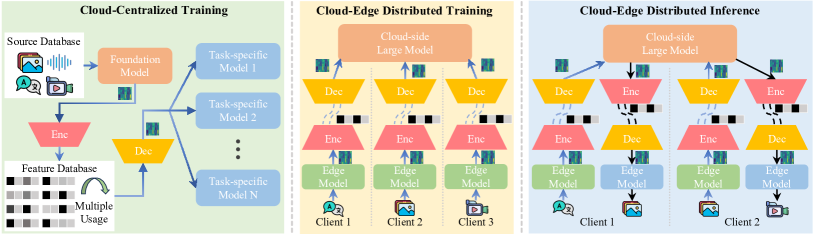
Figure 1: Three application scenarios for feature coding in large model deployment. Cloud-centralized training: Features generated by foundation models are encoded and stored in a feature database. This database supports various downstream tasks, reducing computational demands by avoiding repeated inference of large foundation models. Cloud-edge distributed training: To protect user data privacy, raw data is first processed by an edge model to generate features, which are then encoded and transmitted to the cloud. The cloud decodes these features to complete the remaining forward propagation. Cloud-edge distributed inference: A large model is partitioned across multiple parts, with portions offloaded to edge devices to distribute the computational load. The transmitted features ensure privacy protection and enable customized downstream tasks. Please refer to Sec. 3 for detailed illustrations.

1 Introduction

Large models have revolutionized artificial intelligence (AI) with their impressive performance. However, they require substantial training data and extensive computational resources, posing significant challenges for practical deployment [18]. To address these challenges, distributed deployment has been proposed as a promising solution [32, 37, 43, 46, 22, 14]. By distributing the computational workload across multiple platforms, this approach reduces resource strain on individual systems and enables the integration of private client data into training while maintaining data security [43, 4]. As model scale continues to grow, distributed deployment is expected to become a mainstream strategy for large model applications.

In distributed deployment, effective information exchange between model segments is essential. During forward propagation, features act as information carriers, passing features generated by early segments to later segments to complete inference. Given the vast amount of data in large model applications, encoding features to a smaller size to reduce storage and transmission burden is necessary. Analogous to image and video coding, feature coding has been proposed to address this problem [6, 17, 16, 38].

Existing feature coding research has three key limitations: narrow model types, limited task diversity, and constrained data modalities. Most existing feature coding efforts focus on small-scale, convolution-based networks, such as ResNet, ignoring large models. Although discriminative models, such as DINOv2 [28] and SAM [20], represent a significant branch of large models, they are still underrepresented in feature coding research. Generative models also have received little attention in this area. Furthermore, existing research primarily targets visual features, with limited integration of features from large language models (LLMs) based on textual inputs. This gap indicates a need for broader exploration across both model and data modalities to advance feature coding.

In this work, we shift feature coding research from small-scale to large-scale models. To address the existing limitations, we construct a comprehensive test dataset with features from five tasks across three large models, covering both visual and textual data for increased modality diversity. Using this dataset, we establish unified test conditions to enable fair coding performance comparisons, including formulated bitrate computation and task-specific evaluation pipelines.

To establish a foundation for large model feature coding, we propose two baseline methods and evaluate them on our dataset. The baselines leverage two primary image coding techniques: the handcrafted VVC Intra coding [2] and the learned Hyperprior method [1]. For each method, we introduce pre-processing and post-processing modules tailored to feature coding. Our analysis provides insights into baseline performance and highlights promising research directions.

In summary, our main contributions are as follows:

• We emphasize the importance of feature coding in large model deployment, identifying relevant application scenarios and extending feature coding research from small- to large-scale models.

• We construct a diverse feature dataset encompassing three model types, five tasks, and two data modalities, along with unified test conditions to support future feature coding research.

• We propose and benchmark two feature coding methods on the dataset, offering baseline evaluations and insights for future research in this field.

Model	Parameters	Task	Split Point	Feature Shape	Source Data
DINOv2	1.1B	Image Classification	$40^{th}$ ViT Block	$257\times 1536$	ImageNet, 100 samples
		Semantic Segmentation	$40^{th}$ ViT Block	$2\times 1370\times 1536$	VOC2012, 20 samples
		Depth Estimation	$10^{th}$, $20^{th}$, $30^{th}$, $40^{th}$ ViT Blocks	$2\times 4\times 1611\times 1536$	NYU-Depth-v2, 16 samples
Llama3	8B	Common Sense Reasoning	$32^{th}$ Decoder Layer	$N\times 4096$	Arc-Challenge, 100 samples
SD3	8B	Text-to-Image Synthesis	Input Layer of VAE Decoder	$16\times 128\times 128$	COCO2017, 100 samples

Table 1: Summary of the model and task selection, split point decision, and source data collection.

2 Background and motivation

2.1 Feature coding

Visual signal coding encodes and reconstructs the original visual data [33, 44, 15, 25, 34]. Unlike visual signal coding, feature coding refers to the process of encoding features into bitstreams. Originally introduced within the Coding for Machines framework [42, 10], feature coding is one of two primary branches alongside visual coding. One step in time ahead of feature coding, visual signal coding has already been explored in the context of large models [35].

Despite recent progress, feature coding research currently faces three limitations. First, there is a restricted variety of model types in use. The existing feature extraction relies on small-scale, CNN-based models such as ResNet series [23, 31, 19, 24, 3]. However, as Transformer architectures now dominate large model research [36, 11, 12, 28], it is crucial to investigate feature coding for Transformer-based models to capture the rich representations they provide. Second, the field is constrained by the limited scope of task types. Existing studies mainly address discriminative tasks like image classification and segmentation [7, 13, 45, 41, 5, 27], while generative tasks remain largely unexplored. Given the significance of generative models in modern AI, extending feature coding to include these tasks, such as image synthesis, is essential. The third limitation is the constrained range of source modalities. Current feature coding research predominantly focuses on features from visual data, overlooking the increasingly important features derived from textual data, particularly in light of advancements in LLMs. Expanding to multiple modalities is crucial as the diversity of AI applications grows.

Additionally, two core challenges hinder progress in feature coding for large models: the lack of a public test dataset and unified test conditions. Without a standardized dataset and evaluation conditions, fair comparisons across methods are not feasible. A public dataset ensures consistent input data across studies, while unified test conditions establish a consistent benchmark for evaluating performance.

These limitations motivate us to develop a diverse test dataset and formulate unified test conditions to advance feature coding research.

2.2 Large model deployment

The impressive performance of large models is driven by scaling laws [29, 30], which emphasize the importance of vast model sizes and extensive training data. For example, GPT-3 was built with 175 billion parameters and trained on 499 trillion tokens, both contributing to substantial computational demands. To alleviate these resource requirements, distributed training and inference methods have been proposed in [43, 46, 14].

User privacy presents another critical challenge in client services [4, 26, 40]. Split learning has been introduced as a solution, effectively protecting training data privacy by dividing computation between clients and clouds [43].

In distributed deployment, efficient information exchange between model segments is essential. However, the academic focus has largely overlooked the storage and transmission costs of exchanging these features. Motivated by this gap, our work encodes features into bitstreams to streamline storage and transmission, addressing an essential component of efficient distributed deployment for large models.

3 Feature coding in large models

This section presents three application scenarios of feature coding in large model deployment, illustrated in Fig. 1. Each scenario highlights the role of feature coding in optimizing deployment efficiency.

3.1 Large model training

Large models achieve their high performance through extensive training on large-scale datasets. Due to the limited computational capacity of edge devices, cloud-centralized training is commonly utilized. However, in sensitive domains like healthcare, high-quality public data may be scarce, necessitating access to private data through cloud-edge collaborative training.

3.1.1 Cloud-centralized training

In cloud-centralized training, source databases are maintained in the cloud, where intensive computational demands is the main challenge. Increasingly, complex tasks are addressed through the collaborative use of multiple models. For instance, in vision-language tasks, visual data is initially processed by a vision model, and its features are subsequently passed to an LLM for advanced reasoning. Similarly, foundation models often serve as core backbones for a range of tasks. For example, features extracted from DINOv2 are repurposed for downstream tasks like segmentation [9]. In such collaborative workflows, features generated by one model become input to other models. However, during training, each data sample may undergo repeated inference through the foundation model, leading to a substantial unnecessary computational load.

To mitigate this, an effective solution involves generating features once, storing them, and reusing them across tasks. The workflow is outlined on the left of Fig. 1. First, a foundation model extracts features from the source database, which are then encoded and stored in a feature database. For subsequent task-specific training, only the precomputed feature database is needed, enabling efficient access to features without redundant feature extraction. This significantly reduces computational load and accelerates the training of downstream tasks. However, raw feature data requires substantial storage space, especially with large datasets. To address this, we propose using feature coding to compress raw features into compact bitstreams, reducing storage demands and facilitating efficient, large-scale training.

$SP_{DM1}$

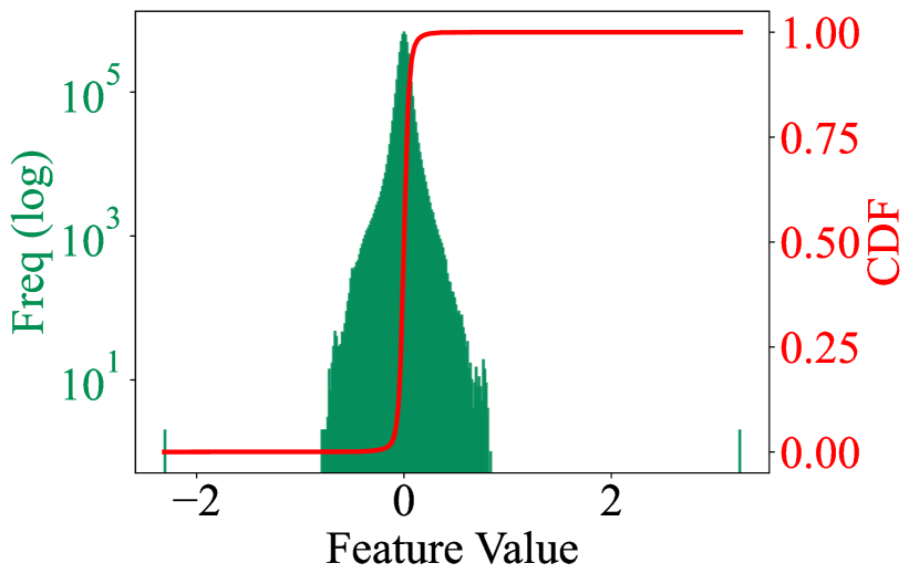
$SP_{DM2}$

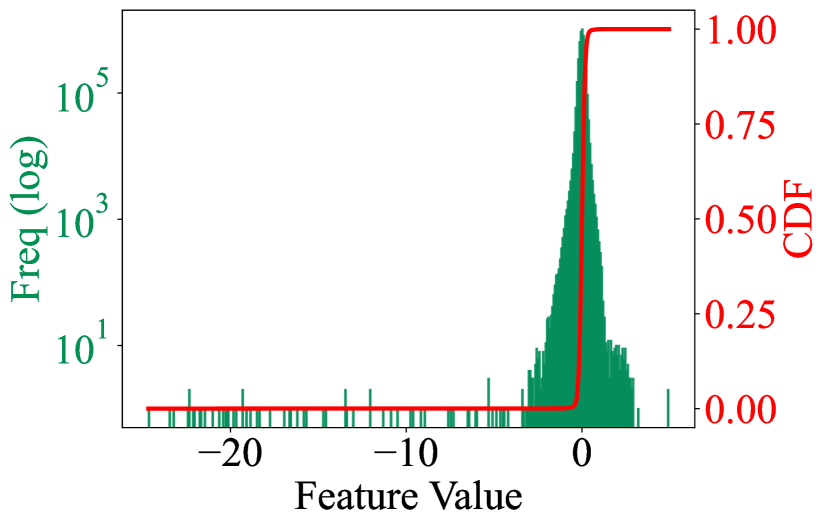
$p2$

$p3$

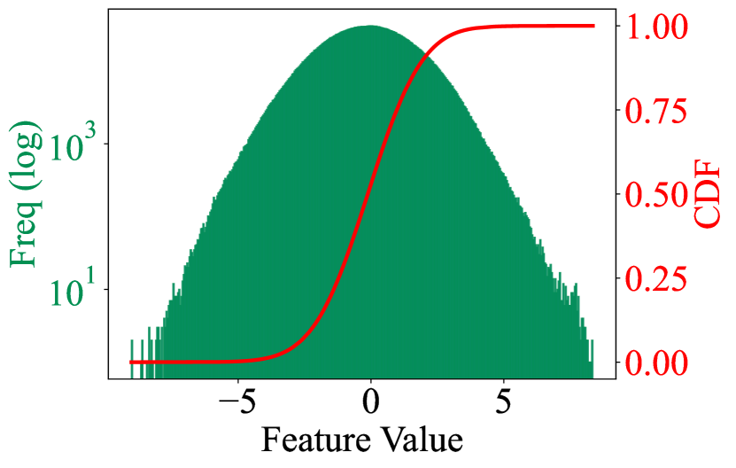
$SP_{DM3}$

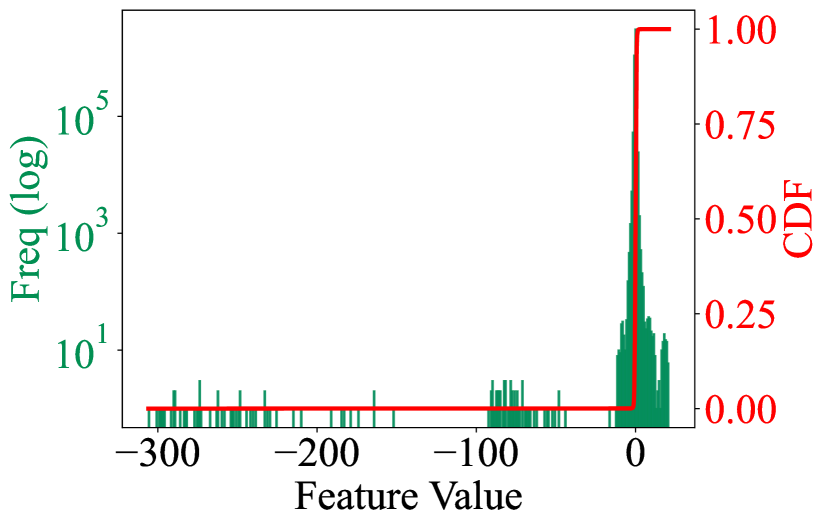
$SP_{DM4}$

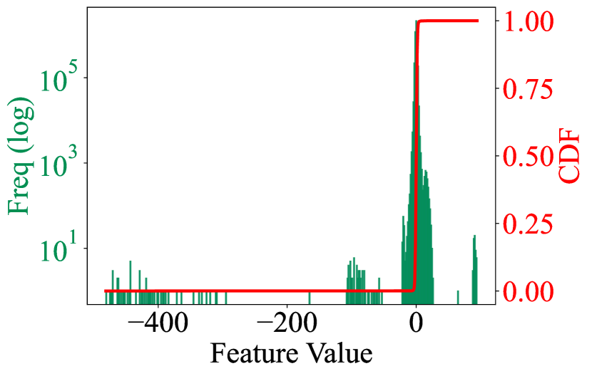
$p4$

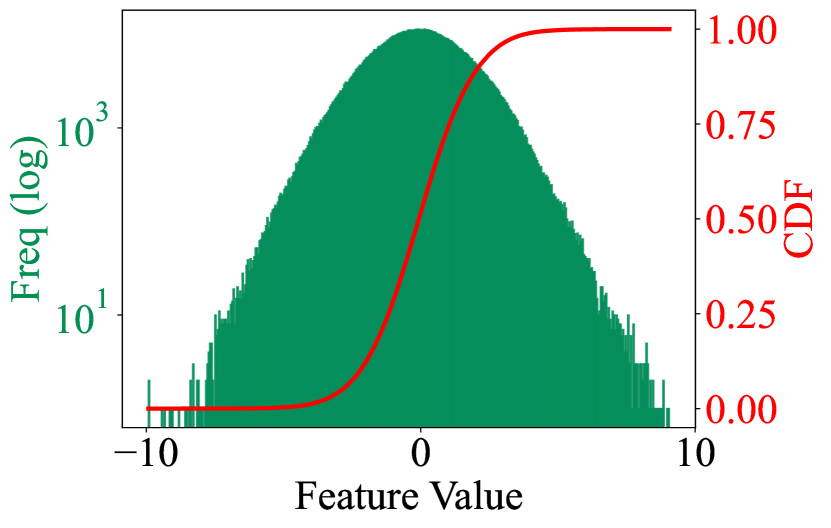
$p5$

$SP_{GS}$

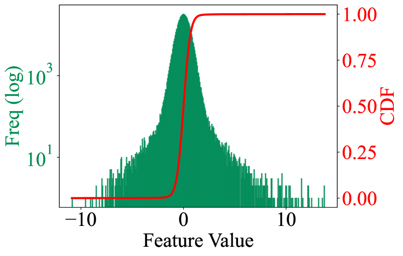
$SP_{H}$

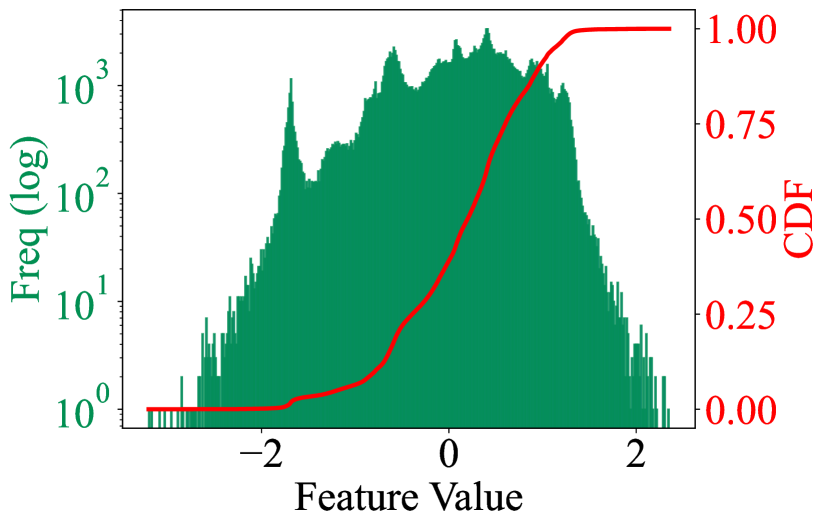
$C5$

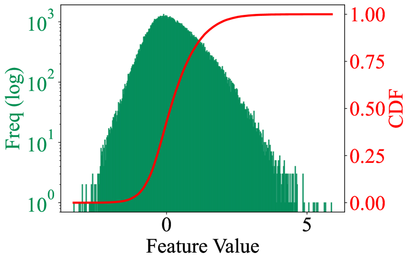
$C5$-ReLU

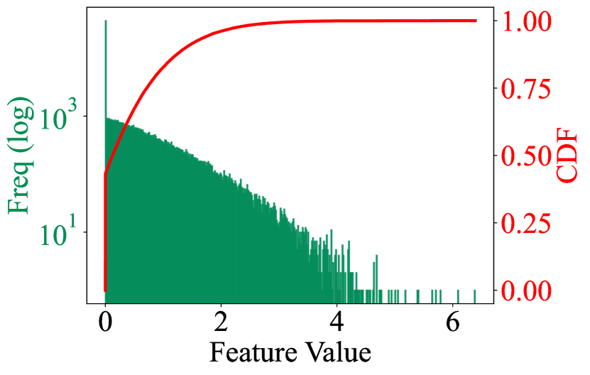
Figure 2: Frequency and CDF comparisons between features in the proposed dataset and commonly used existing features. The proposed features exhibit distinct distributions compared to existing features, highlighting the necessity and value of the dataset. In addition, the proposed features demonstrate greater diversity, enhancing their representativeness and suitability for long-term use. Frequencies are scaled logarithmically for better visualization.

3.1.2 Cloud-edge distributed training

In addition to computational resources, large model training demands access to large-scale datasets, which are often only available to a few giant high-tech companies. Furthermore, sensitive data, such as medical records and financial information, cannot be freely shared due to privacy concerns and regulatory constraints. To leverage distributed, privately owned data, split learning has emerged as a viable solution [37]. Split learning divides the training process into two phases, with the bulk of the computational load handled by the cloud, while edge devices, which are often resource-constrained, handle a smaller portion of the task. This approach minimizes the computational demand on the edge while enabling collaboration with powerful cloud resources.

The cloud-edge distribution training pipeline is depicted in the second diagram of Fig. 1. The whole pipeline is divided into two parts: edge models and cloud-side large models. During forward propagation, the edge model processes private data to generate features, which are then encoded into bitstreams and transmitted to the cloud. Upon receiving the bitstreams, the cloud decodes them back into features and feeds them into the large model. In the backward pass, gradients are computed and backpropagated along the reverse path. To optimize this process (reduce bandwidth usage and minimize transmission time), it is critical to apply feature coding before transmission.

3.2 Cloud-edge distributed inference

Once large models are trained, they are deployed in products to provide client services. For a product or service to succeed, two primary concerns must be addressed: supporting a high volume of simultaneous cloud server access and protecting user privacy. For the first concern, managing computational load is essential, particularly in generative applications that involve repetitive diffusion processes. A practical solution is to offload part of this computational demand to edge/client devices. For the second concern, the same strategy in the cloud-edge distributed training, as discussed in Sec. 3.1.2, can apply.

The cloud-edge distributed inference pipeline is illustrated in the diagram on the right of Fig. 1. In the upload phase, source data is converted into features by an edge model on the client side. These features are then encoded and transmitted to the cloud, where they are further processed by large models. In the download phase, the processed features are sent back to the client to complete a specific task. Depending on the task head used, various functionalities can be performed with the returned features. For example, Stable Diffusion 3 (SD3) features derived from an image can be used to synthesize video or generate segmentation masks. This approach not only reduces the computational load on the cloud server but also enhances data privacy by keeping raw user data on the edge/client side.

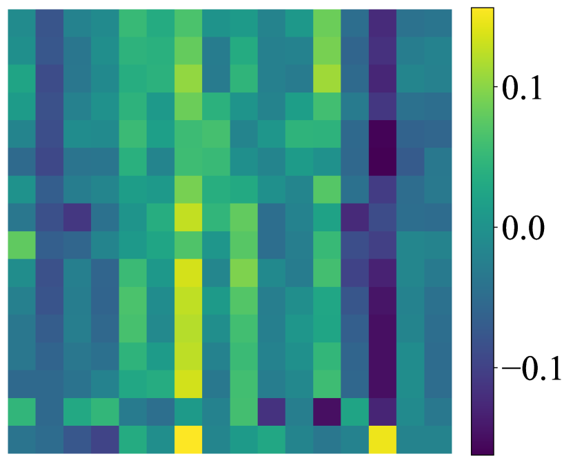
$SP_{DM1}$

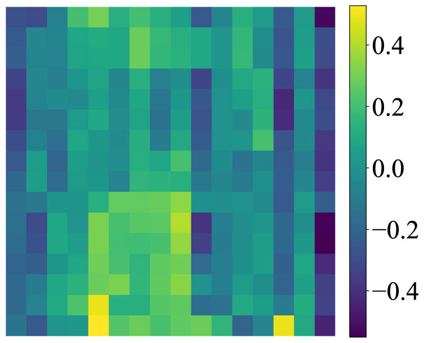
$SP_{DM2}$

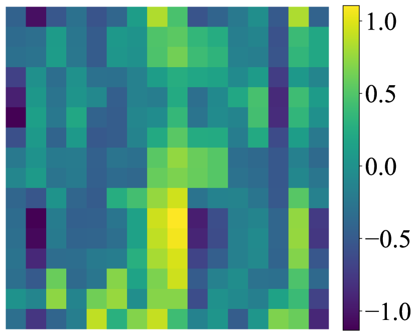
$SP_{DM3}$

$SP_{DM4}$

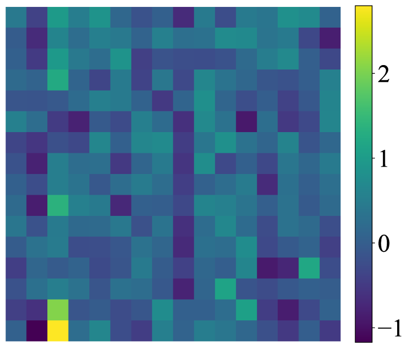
$SP_{GS}$

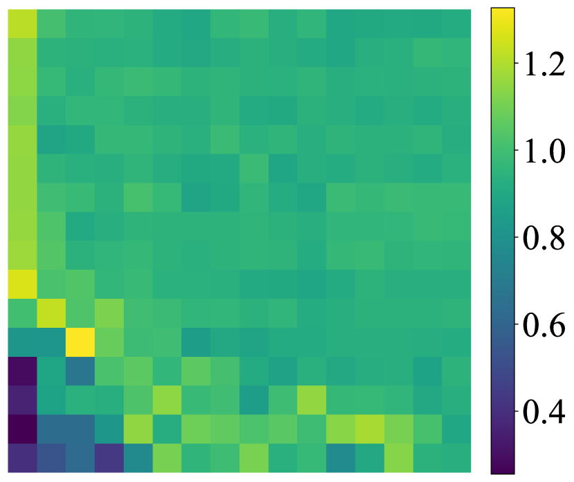
$SP_{H}$

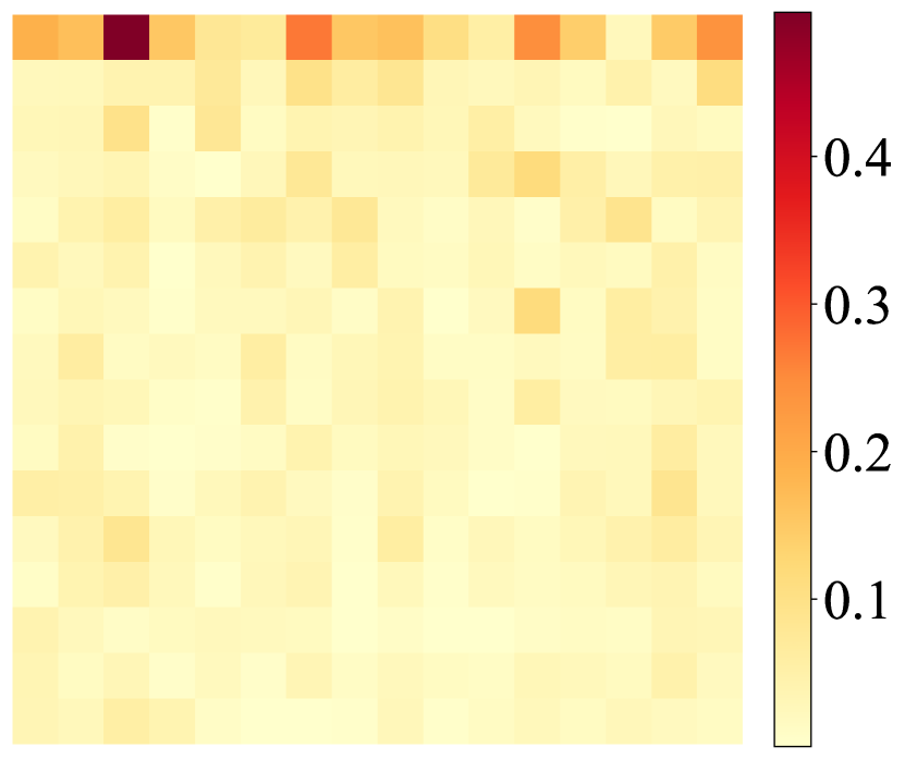
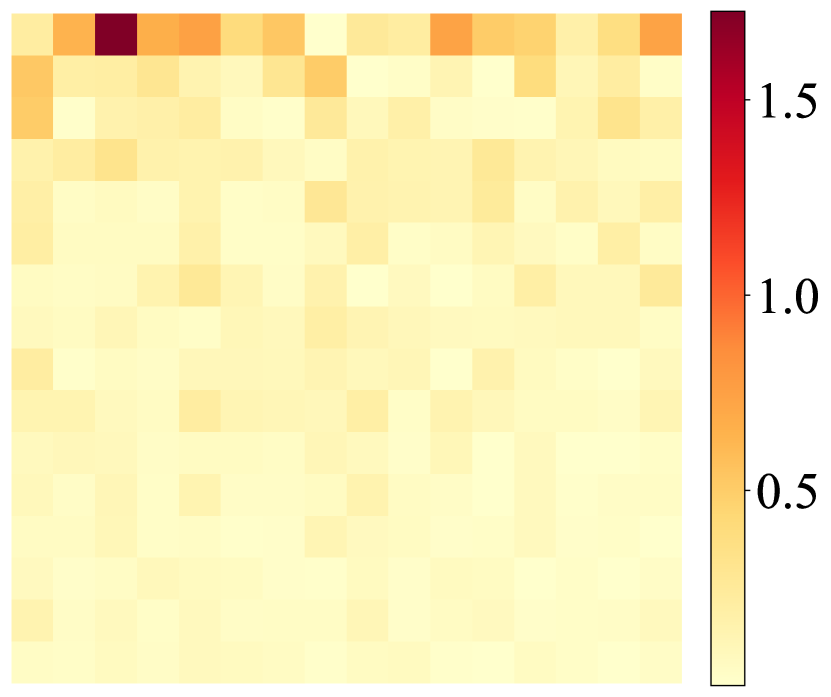
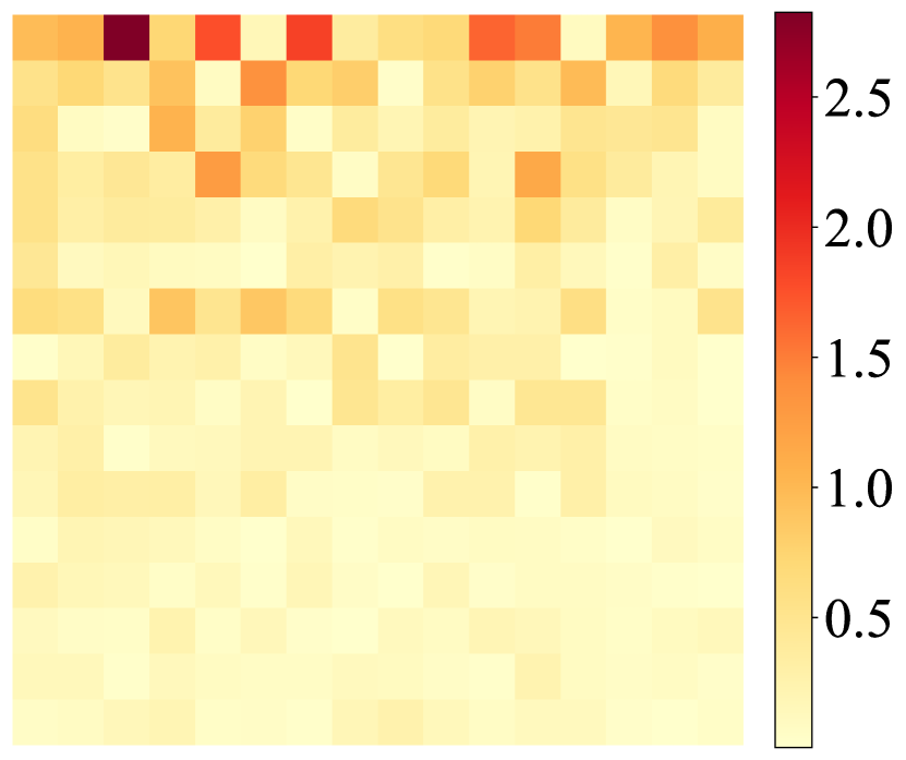
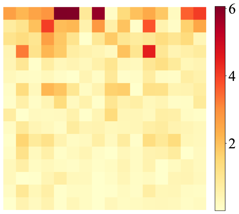
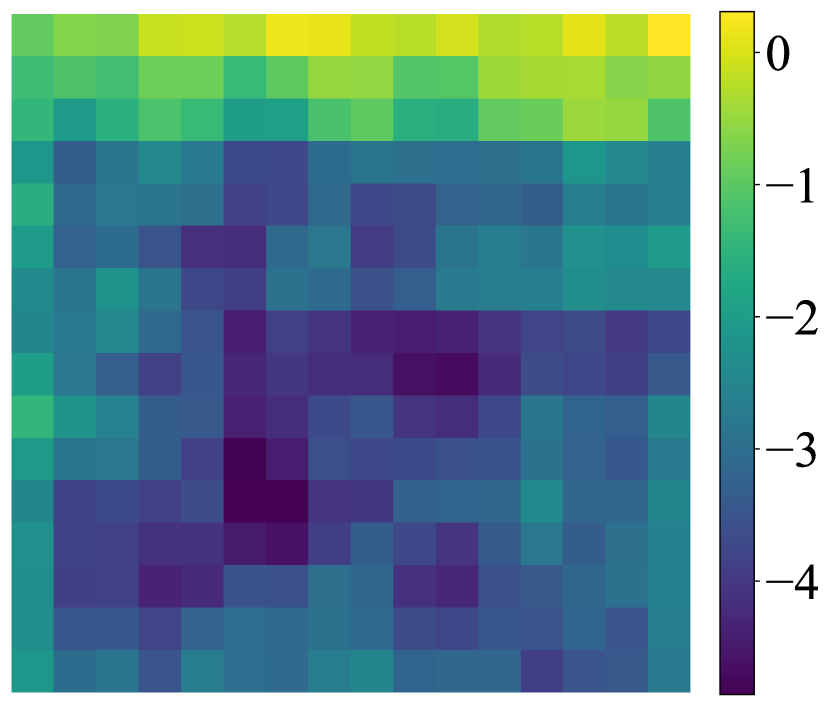
$p2$

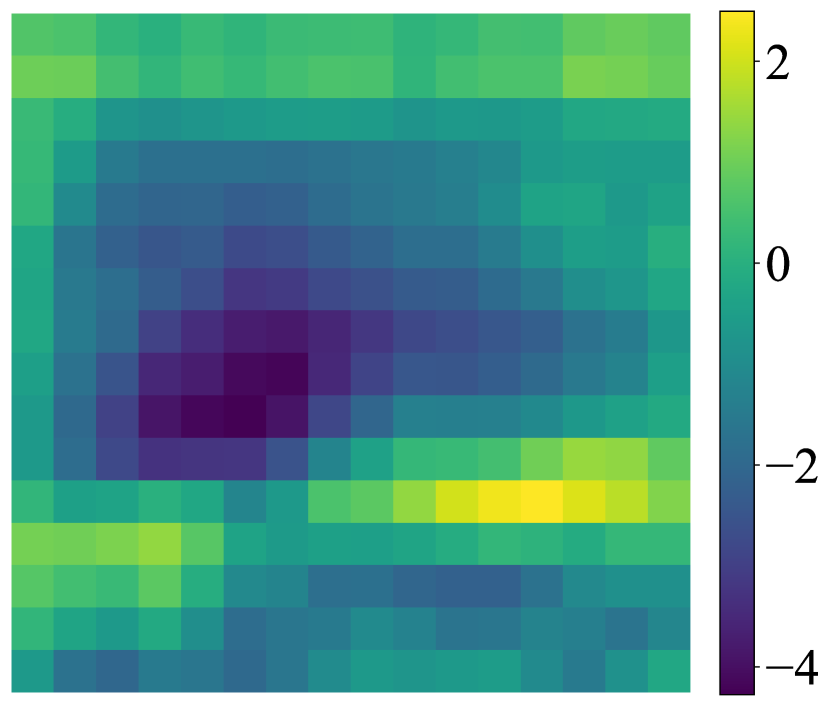
$p3$

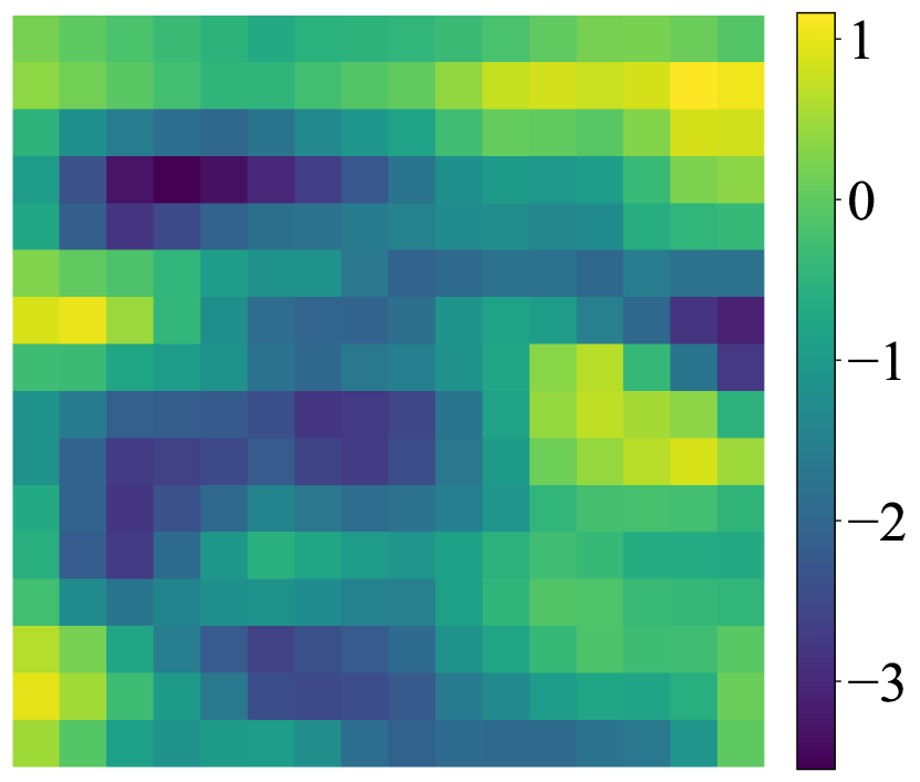
$p4$

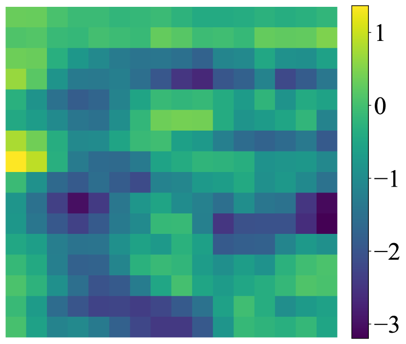
$p5$

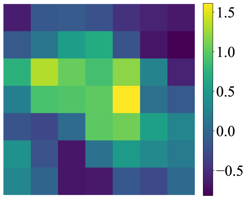
$C5$

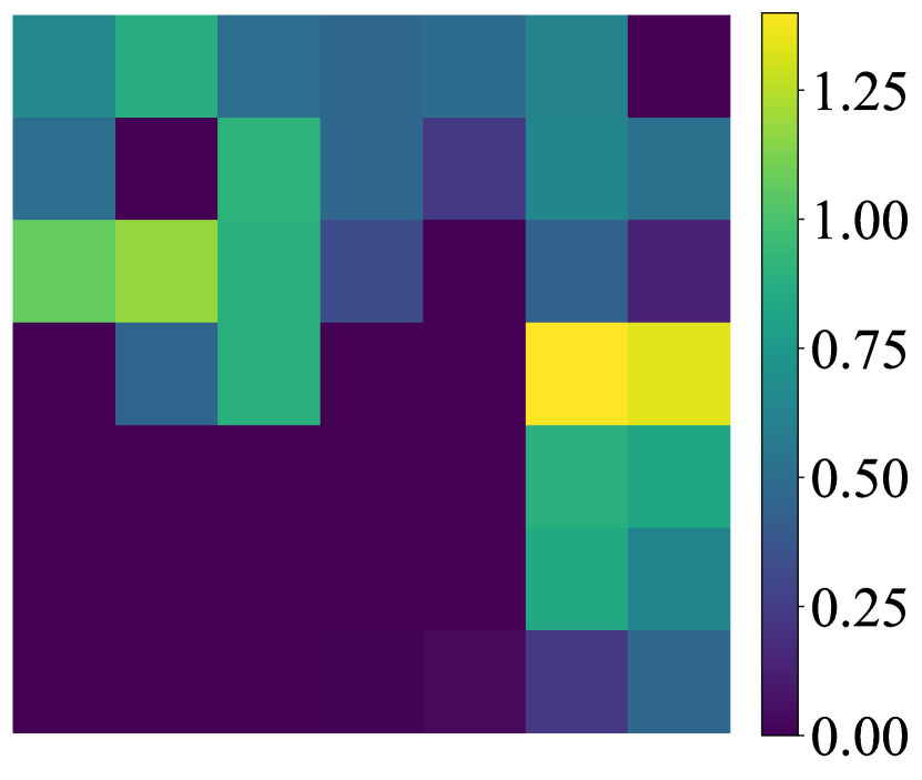
$C5$-ReLU

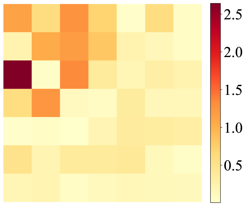
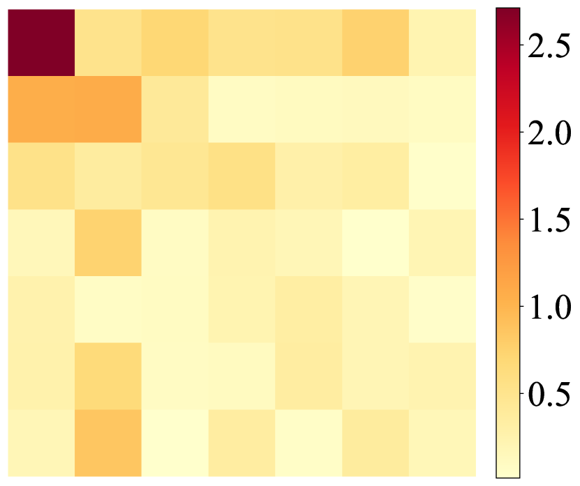
Figure 3: Visualization of the original feature blocks and their corresponding DCT blocks (absolute values). In the feature domain, the proposed features exhibit higher vertical redundancy, whereas the existing features vary smoothly in both directions. In the DCT domain, the proposed features display more dispersed energy distributions. These distinct redundancy characteristics indicate different coding properties.

4 Dataset construction and analysis

4.1 Dataset construction

To guarantee the dataset’s representativeness and support the long-term study of feature coding research, we curate the test dataset with consideration of three key aspects. Table 1 outlines our selected models and tasks, split points, and source data.

4.1.1 Model and task selection

This study expands the scope of feature coding research by encompassing discriminative, generative, and hybrid models. While prior work has primarily concentrated on discriminative, convolution-based models, the advent of Transformer architectures and generative models calls for a more comprehensive dataset to capture a wider range of tasks and feature types. To meet this need, we select three representative models: DINOv2 [28], Llama3 [11], and SD3 [12]. Llama3 and SD3 represent two core categories within generative models, highlighting their respective strengths in different input-output modalities. Specifically, DINOv2 and Llama3 handle visual and textual inputs, while SD3 processes textual inputs to generate visual outputs. The selected models offer comprehensive feature representations across visual, textual, and cross-modal applications.

For DINOv2, we include the image classification, semantic segmentation, and depth estimation tasks. Llama3 addresses the common sense reasoning task, and SD3 focuses on text-to-image synthesis. This selection covers three visual tasks, one textual task, and one text-to-visual task, forming a versatile foundation for feature coding analysis across diverse task and model types.

4.1.2 Split point decision

This section describes the selection of split points for each model. For DINOv2, we define two types of split points: 1) $SP_{DS}$, the output of the $40^{th}$ ViT layer, and 2) $SP_{DM}$, which aggregates outputs from the $10^{th}$, $20^{th}$, $30^{th}$, and $40^{th}$ ViT layers. $SP_{DS}$ is used for tasks utilizing single-layer features, while $SP_{DM}$ supports tasks that require multi-layer features. In this study, $SP_{DS}$ is applied to image classification and semantic segmentation, and $SP_{DM}$ to depth estimation. The resulting features are designated as $F_{Cls}$, $F_{Seg}$, and $F_{Dpt}$, respectively.

For Llama3, the split point $SP_{G}$ is set at the output of the $32^{nd}$ decoder layer. Features extracted at $SP_{G}$ are versatile, supporting both task-specific heads and integration with other large models [39]. In the common sense reasoning task, $SP_{G}$ produces features of size $N\times 4096$, where $N$ represents the number of tokens.

For SD3, we establish the input layer of the VAE decoder as the split point $SP_{H}$. This split point generates features of size $16\times 128\times 128$, denoted as $F_{TTI}$, which are then passed to the VAE decoder for image synthesis.

4.1.3 Source data collection

Inspired by the video coding standard VVC [2], where test sequences are divided into 8 classes with 3–5 video sequences each, we organize our feature test dataset into five categories. Each category is supported by a curated subset of public datasets used as source data.

For image classification, we select 100 images from ImageNet [8], each representing a unique class accurately classified by DINOv2. For semantic segmentation, we collect 20 images from VOC2012, ensuring coverage of all 20 object classes. For depth estimation, we source 16 images from NYU-Depth-v2, adhering to the train-test split proposed in [21] and selecting one image for each scene category. In the common sense reasoning task, we utilize 100 samples from Arc-Challenge dataset, chosen for their longest input prompts and correct prediction by Llama3. For text-to-image synthesis, we first select 100 images from COCO2017 and then collect their longest captions.

4.2 Feature analysis

In this section, we analyze and compare the proposed features with those commonly used in existing research to clarify the necessity and importance of proposing a new dataset.

4.2.1 Distribution analysis

Frequency distributions and cumulative distribution functions (CDFs) of the proposed and commonly used existing features are visualized in Fig. 2. Features $C5$ and $C5$-ReLU are derived from Pytorch official ResNet50 pre-train on ImageNet, while $P$ features (including $p2$, $p3$, $p4$, and $p5$) are generated by the ResNeXT101-based MaskRCNN pre-trained on COCO2017.

The proposed features exhibit distinct distributions compared to existing features, underscoring the necessity and value of the dataset. For multi-layer split points, four key distinctions between $SP_{DM}$ and $P$ are observed: (1) $SP_{DM}$ distribution range expands progressively with deeper layers; (2) $SP_{DM}$ distribution is more asymmetric; (3) $SP_{DM}$ feature values are more concentrated, as shown in the CDFs; and (4) $SP_{DM}$ features contain more regions with sparse feature points. For single-layer split points, $SP_{GS}$ has a more concentrated distribution, while $SP_{H}$ shows more peaks. Unlike $C5$-ReLU, the proposed dataset omits similar features, as ReLU is infrequently used in large models.

The proposed features demonstrate the high diversity of the dataset, enhancing its representativeness and suitability of long-term research.

Task	Head	Metric
Cls	Norm + Linear1	Accuracy
Seg	Norm + Linear1	mIoU
Dpt	Linear4	RMSE
CSR	Norm + Linear + Softmax	Accuracy
TTI	VAE Decoder	CLIP Score

Table 2: Summary of task head and accuracy metric settings. Specific definitions of Heads can be found in the original papers [28, 11, 12].

4.2.2 Redundancy analysis

We conduct a redundancy analysis on feature blocks, using $7\times 7$ blocks for $C5$ and $C5$-ReLU and $16\times 16$ blocks for other features. We visualize the original feature blocks and their DCT blocks (absolute values) in Fig. 3. In the feature domain, clear spatial redundancy is observed in both $SP_{DM}$ and $SP_{H}$ features, with $SP_{H}$ exhibiting redundancy in both horizontal and vertical directions, while $SP_{DM}$ shows stronger vertical redundancy. By contrast, $SP_{GS}$ features vary rapidly in both directions, resulting in weak spatial redundancy. This is because Llama3 only processes textual data, which lacks inherent spatial correlation. In comparison, existing features exhibit smoother spatial variation and thus high spatial redundancy. We attribute this to the translation invariance of convolutional layers, which preserve the relative positions of pixels in the feature domain, resulting in consistent redundancy patterns. In contrast, transformer-based vision models partition images into patches before transforming them, shifting spatial redundancy primarily to the vertical direction, as seen in $SP_{DM}$.

In the DCT domain, the spatial redundancy is reflected by energy distribution: the proposed features display more distracted energy, whereas existing features concentrate energy in the top-left DC component. Notably, $SP_{H}$ has the highest energy concentration, as it looks similar to images.

The distinct redundancy characteristics indicate different requirements for feature coding methods, which should be explored in future studies.

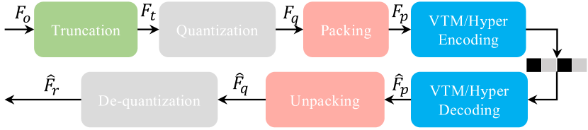
Figure 4: The pipeline of the proposed baseline feature coding method. The quantization and de-quantization modules are only used in the VTM baseline.

Task	Image Classification			Semantic Segmentation			Depth Estimation			Common Sense Reasoning			Text-to-Image Synthesis
Metric	BPFE	Accuracy	MSE	BPFE	mIoU	MSE	BPFE	RMSE	MSE	BPFE	Accuracy	MSE	BPFE	CLIP Score	MSE
Quantization	10	100	2.8974	10	79.93	1.8135	10	0.4941	0.5737	10	100	0.0042	10	30.07	0.00001
VTM Baseline	1.90	100	3.0117	1.78	79.68	1.9279	1.67	0.5341	0.6103	2.69	99	0.0114	1.30	30.04	0.0029
	0.98	99	3.2324	0.90	78.91	2.1438	0.79	0.6925	0.6763	1.83	100	0.0267	0.65	29.95	0.0078
	0.21	81	3.7424	0.24	73.53	2.6032	0.24	1.0684	0.8033	0.88	98	0.0826	0.26	29.50	0.0171
	0.04	18	4.0751	0.04	55.05	3.0304	0.05	1.4053	0.9302	0.16	81	0.1900	0.10	27.43	0.0290
	0.01	2	4.4588	0.01	32.64	3.3641	0.01	1.5542	1.0313	0.04	26	0.2483	0.04	24.42	0.0436
Hyperprior Baseline	1.99	92	3.5279	1.72	78.44	2.2636	1.51	0.5691	0.6588	5.50	95	0.0674	1.40	30.20	0.0054
	1.11	91	3.7724	1.30	77.85	2.3423	1.01	0.6410	0.6830	2.84	89	0.0796	0.62	29.55	0.0122
	0.89	86	3.9035	0.54	76.39	2.6461	0.43	0.9442	0.7818	1.46	83	0.1474	0.26	28.21	0.0216
	0.37	29	4.3309	0.12	62.69	3.0935	0.08	1.1809	1.0830	1.30	67	0.1337	0.14	26.68	0.0294
	0.23	11	4.8063	0.03	40.92	3.6286	0.01	2.5775	1.1876	1.19	32	0.1582	0.07	24.27	0.0404

Table 3: Rate-accuracy performance evaluations on the two baseline methods (MSE is calculated between $F_{o}$ and $\hat{F}_{r}$).

5 Unified test conditions

Even with a test dataset, fair comparisons are still challenging without identical test conditions. To address this, we establish unified test conditions here.

5.1 Bitrate computation

We introduce a new bitrate measurement, Bits Per Feature Point (BPFP), replacing the commonly used Bits Per Pixel (BPP). BPFP is calculated by dividing the total coding bits by the number of feature points.

Our rationale for shifting from BPP to BPFP is twofold. First, BPP is unsuitable for features extracted from non-visual data where pixels do not exist. Second, we believe bitrate should reflect the actual encoded data (the feature itself) rather than the source data. Using BPP to calculate bitrate on source data introduces ambiguity and limits fair comparisons between coding methods. For instance, applying the same BPP to different features extracted from the same image can be misleading. In addition, BPP may incentivize downscaling source images to reduce feature size, yielding lower bitrates that do not represent true coding efficiency. In contrast, BPFP measures bitrate on the feature itself, enabling fair comparisons across coding methods as long as the same feature is used.

5.2 Task accuracy evaluation

To isolate the impact of task heads on task accuracy, we fix their parameters during evaluation. All task head weights are loaded from pre-trained models. The task heads and accuracy metrics are presented in Table 2.

Task	Split Point	Org. Region	Trun. R. (VTM)	Trun. R. (Hyperprior)
Cls	$SP_{DS}$	[-552.45, 104.18]	[-20, 20]	[-5, 5]
Seg	$SP_{DS}$	[-530.98, 103.22]	[-20, 20]	[-5, 5]
Dpt	$SP_{DM1}$	[-2.42, 3.28]	[-1, 1]	[-1, 1]
	$SP_{DM2}$	[-26.89, 5.03]	[-2, 2]	[-2, 2]
	$SP_{DM3}$	[-323.30, 25.05]	[-10, 10]	[-10, 10]
	$SP_{DM4}$	[-504.43, 102.03]	[-20, 20]	[-10, 10]
CSR	$SP_{G}$	[-78.00, 47.75]	[-5, 5]	[-5, 5]
TTI	$SP_{H}$	[-4.09, 3.05]	[-4.09, 3.05]	[-4.09, 3.05]

Table 4: Summary of the original and truncation region settings.

6 The proposed baselines and benchmark

6.1 The baseline methods

The pipeline for the proposed feature coding methods is illustrated in Fig. 4. First, the original feature $F_{o}$ is truncated to a smaller range. The quantization operation is performed accordingly. Next, the quantized $F_{q}$ is packed into a 2D feature $F_{p}$. The encoder takes $F_{p}$ as input and outputs decoded feature $\hat{F}_{p}$, which is then unpacked to $\hat{F}_{q}$. $\hat{F}_{q}$ is converted back into a floating-point feature $\hat{F}_{r}$. We propose two baselines: a traditional coding method based on VTM and a learned coding method using the Hyperprior approach.

6.1.1 Pre-processing and post-processing

We propose two pre-processing operations: truncation and quantization. The truncation operation is designed to remove feature points that deviate significantly from the central region. The specific truncated regions for each task are listed in Table 4. Please note that different truncations are used for the two baselines for their distinct coding strategies. The quantization operation uniformly quantizes the truncated features to 10-bit integers. The post-processing only performs de-quantization, which is an inverse process of quantization.

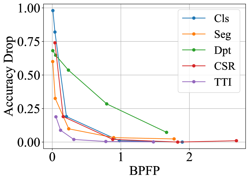
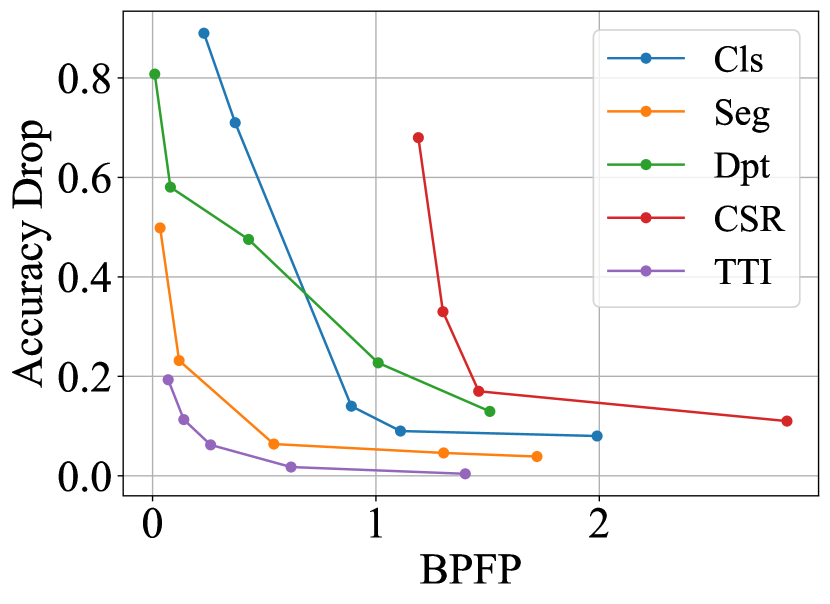
Figure 5: Rate-accuracy-drop comparisons among different tasks. Left: VTM baseline. Right: Hyperprior baseline.

6.1.2 Packing and unpacking

Given the input requirement of VTM, we pack the features into a 2D YUV-400 format. For the Hyperprior encoder, we take the same packing to align with the VTM encoder. $F_{Seg}$, $F_{Dpt}$, and $F_{TTI}$ are packed into the shapes of $2740\times 1536$, $3222\times 6144$, and $512\times 512$, respectively. Please refer to supplementary materials for the packing details.

6.1.3 Encoding and decoding

For the VTM baseline, we employ the VVC reference software VTM-23.3 for feature coding. The Intra coding is applied using the main configuration file encoder_intra_vtm.cfg. The InputChromaFormat is set to 400, and ConformanceWindowMode is enabled. The InternalBitDepth, InputBitDepth, and OutputBitDepth are all set to 10. All other configurations are set to default. In our experiments, five QPs (22, 27, 32, 37, 42) are used.

For the Hyperprior baseline, we modify the input and output to accommodate the 2D features. In addition, we normalized all truncated features into a consistent region of [0,1] before training. Please find detailed training details in the supplementary.

6.2 Rate-accuracy analysis

The rate-accuracy evaluation results are presented in Table 3. We also provide the rate-accuracy curves in the supplementary materials. To further assess the effect of bitrate on accuracy, we introduce a new metric, accuracy drop, defined as the percentage decrease in accuracy. For depth estimation, the reciprocal of RMSE is employed. The bitrate-accuracy-drop curves, shown in Fig. 5, reveal that most tasks exhibit an inflection point where accuracy starts to decrease significantly. However, for depth estimation, this point is observed only in the Hyperprior baseline. In the Hyperprior baseline, inflection points are more distracted across tasks, which may caused by the fact that different models are trained for different tasks. Unlike other tasks, text-to-image synthesis shows smaller accuracy degradation even at low bitrates.

Codec	Cls	Seg	Dpt	CSR	TTI
VTM Baseline	0.8933	0.8787	0.9904	0.7609	0.9329
Hyperprior Baseline	0.9190	0.9367	0.7741	0.5834	0.9793

Table 5: Linear correlation between MSE and task accuracy.

Configuration	Cls	Seg	Dpt	CSR
Truncation Only	100	81.60	0.4992	100
Quantization Only	99	81.37	0.4982	100
Truncation + Quantization	100	79.93	0.4941	100
Quantization + VTM QP22	0	5.35	1.6085	6

Table 6: Ablations on truncation and quantization operations.

6.3 Distortion-accuracy analysis

In this subsection, we examine the linear correlation between feature MSE and task accuracy. We present the coefficients of determination in Table 5. For the VTM baseline, only depth estimation shows a high linear correlation. We believe this arises from its accuracy is measured by RMSE. However, under the Hyperprior baseline, depth estimation does not exhibit a high correlation because of a significant accuracy drop at the lowest bitrate. The common sense reasoning task exhibits an extremely low linear correlation at both baselines, indicating the different characteristics of textual features. This analysis further supports the conclusion that feature MSE is not a good metric for measuring semantic distortion. Developing effective metrics for semantic distortion remains a critical topic in feature coding.

Image Classification				Semantic Segmentation
[-5, 5]		[-30, 30]		[-5, 5]		[-30, 30]
BPFE	Acc.	BPFE	Acc.	BPFE	mIoU	BPFE	mIoU
2.90	100	0.38	91	2.84	79.83	0.37	76.38
2.05	100	0.06	24	1.98	79.40	0.08	63.46
1.15	100	0.02	14	1.10	78.68	0.01	39.32
Depth Estimation				Common Sense Reasoning
[-5, 5], [-5, 5]		[-20, 20], [-30, 30]		[-2, 2]		[-10, 10]
BPFE	RMSE	BPFE	RMSE	BPFE	Acc.	BPFE	Acc.
1.42	0.6490	0.58	0.8569	3.16	98	0.84	98
0.73	0.9604	0.17	1.1360	2.30	99	0.15	82
0.33	1.2453	0.04	1.3073	1.44	99	0.04	20

Table 7: Ablation results on truncation regions. $SP_{DM1}$ and $SP_{DM2}$ features are truncated into [-1, 1] and [-2, 2] in all cases, respectively.

6.4 Ablation on truncation and quantization

In this subsection, we examine the impact of truncation and quantization on feature coding. Given the VTM baseline’s stability and deterministic properties, we conduct this ablation study on it specifically. As shown in Table 6, truncation and quantization individually result in little task accuracy loss. When both are applied together, task accuracies experience slight decreases. However, applying only quantization leads to a significant accuracy drop.

Without truncation, feature values are often limited to a small subset within the full range of [0, 1023]. In this scenario, during feature coding, the codec’s internal quantization maps the narrow input range to a single value, introducing significant distortion. However, by applying truncation, this range is expanded, helping to reduce distortion caused by the inner quantization. To demonstrate this effect, we test several truncation ranges and encode the truncated features using fixed QPs (27, 32, 37). As presented in Table 7, smaller truncation ranges generally yield higher accuracy but come at the cost of increased bitrates. Therefore, selecting an appropriate truncation range is crucial for balancing the target bitrates and accuracy.

7 Conclusion

In this paper, we highlight the critical role of feature coding in deploying large models and make three contributions to advance this field. First, we construct a comprehensive dataset that covers a wide variety of feature types. Second, we establish unified test conditions to support standardized evaluations and ensure fair comparisons for future studies. Third, we introduce two baseline methods, providing foundational benchmarks and insights for researchers exploring this field.

We identify three promising directions for future feature coding research. First, further improvements in coding performance are encouraged. Second, robust methods for measuring semantic distortion in feature coding deserve more attention. Third, developing generic feature coding methods that can handle diverse features across various models is expected.

Supplementary Material

8 Additional dataset analysis

$SP_{DS},F_{Cls}$

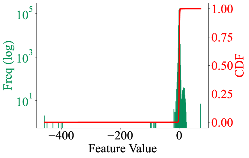
$SP_{DS},F_{Seg}$

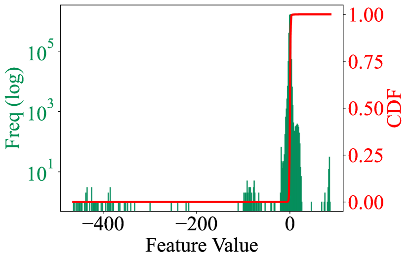
Figure 6: Visualization of the frequency distribution and CDF for the $F_{Cls}$ and $F_{Seg}$ features.

	Proposed Features						Existing Features
Source Dataset	Split Point	Max	Min	Mean	IV	GM	Split Point	Max	Min	Mean	IV	GM
ImageNet	$SP_{DS}$	79.01	-502.04	0.0782	17.04	3.97	$C5$-ReLU	7.81	0	0.4594	9839.49	143.22
VOC2012	$SP_{DS}$	94.88	-485.23	0.0780	13.30	4.30	$C5$	8.00	-4.24	0.2473	7323.72	131.90
NYUv2	$SP_{DM1}$	3.25	-2.33	-0.0015	128.91	17.92	$p2$	10.83	-11.11	-0.1726	8452.88	159.45
	$SP_{DM2}$	4.99	-26.08	-0.0005	36.96	10.00	$p3$	8.35	-9.02	-0.1277	9418.53	168.38
	$SP_{DM3}$	23.51	-314.26	0.0042	9.61	2.76	$p4$	9.06	-9.93	-0.0629	8499.73	158.89
	$SP_{DM4}$	96.04	-493.17	0.0731	12.54	4.35	$p5$	9.61	-8.22	-0.0295	9402.06	169.13
Arc-Challenge	$SP_{GS}$	27.50	-26.38	0.0038	419.14	33.28	/	/	/	/	/	/
Captions from COCO2017	$SP_{H}$	2.19	-1.09	0.5420	22918.26	118.22	/	/	/	/	/	/

Table 8: Statistics of the proposed features and existing features. (Gradient magnitude values are scaled by $10^{5}$).

We visualize the distributions, feature blocks, and DCT blocks of $F_{Cls}$ and $F_{Seg}$ extracted from $SP_{DS}$ in Fig. 6 and Fig. 7. These distributions exhibit high similarities to the features extracted from $SP_{DM4}$, as they are derived from the same layer. To avoid redundancy in the main paper, these visualizations have been moved to the supplementary material.

Additionally, we compare the proposed features with existing features in terms of statistical characteristics, as presented in Table 8. Specifically, we randomly sample 10 examples from each dataset for statistical analysis, reporting the maximum, minimum, and mean values. In general, the proposed features exhibit broader distribution ranges compared to existing features. For multi-scale features, the distribution range expands with deeper network layers, whereas existing features show smaller variation. In addition, although the proposed features are more asymmetric, their mean values are closer to zero.

To assess spatial redundancy, we compute intensity variance (IV) and gradient magnitude (GM), with gradients calculated using the Sobel operator. Prior to computation, pixel and feature values are quantized to 10-bit integers. The intensity variance of the proposed features spans a wide range, from 9.61 to 22918.26, whereas existing features have a narrower range of [7323.72, 9839.49]. A similar trend is observed in gradient magnitude. The larger variations demonstrate the higher diversity of the proposed features. Furthermore, among the proposed features, textual features reveal distinct distribution characteristics compared to visual features. For instance, $SP_{GS}$ and $SP_{H}$ exhibit larger intensity variance and gradient magnitude. This highlights the necessity and importance of including textual features in the proposed dataset.

$SP_{DS},F_{Cls}$

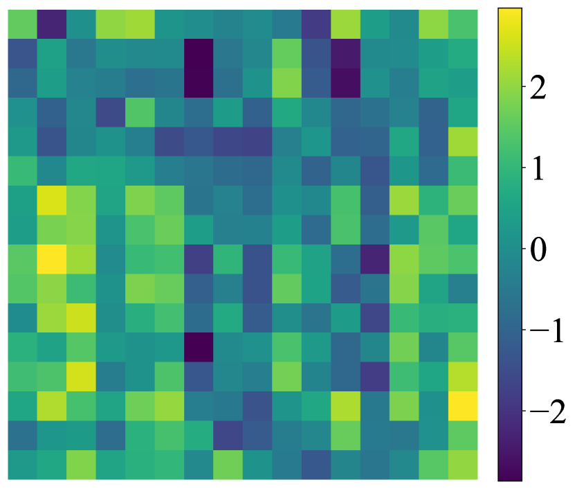
$SP_{DS},F_{Seg}$

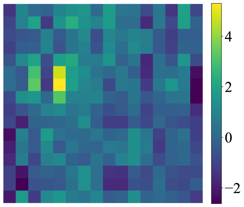
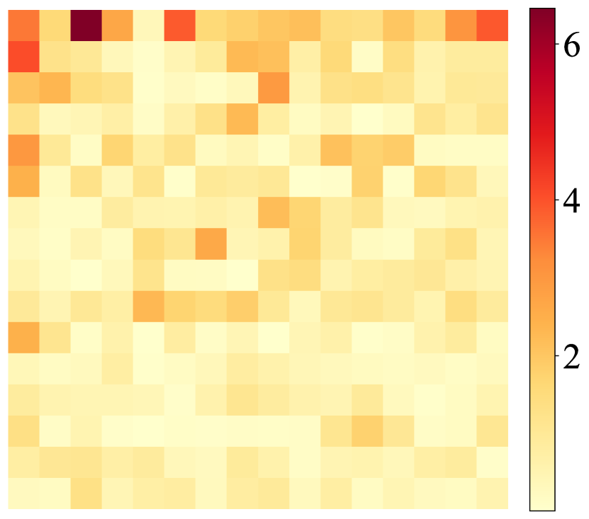
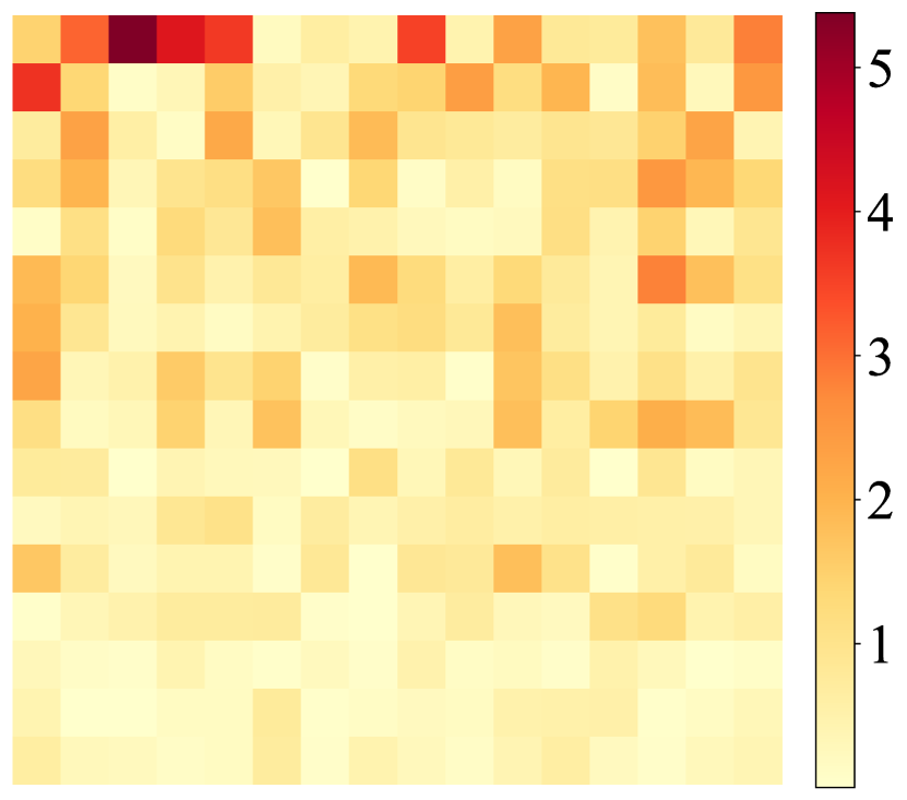
Figure 7: Visualization of the original feature blocks and their corresponding DCT blocks for the $F_{Cls}$ and $F_{Seg}$ features.

Task	Source Dataset	Number of Samples	Feature Shape	Epoch	Learning Rate	Lambda
Cls	ImageNet	5000	$256\times 256$	800	1e-4	0.001, 0.0017, 0.003, 0.0035, 0.01
Seg	VOC2012	5000	$256\times 256$	800	1e-4	0.0005, 0.001, 0.003, 0.007, 0.015
Dpt	NYUv2	20000	$256\times 256$	200	1e-4	0.001, 0.005, 0.02, 0.05, 0.12
CSR	Arc-Challenge, OpenBookQA	6000	$64\times 4096$	200	1e-4	0.01405, 0.0142, 0.015, 0.045, 10
TTI	Captions from COCO2017	50000	$512\times 512$	60	1e-4	0.005, 0.01, 0.02, 0.05, 0.2

Table 9: Training details of the Hyperprior baseline.

Image Classification

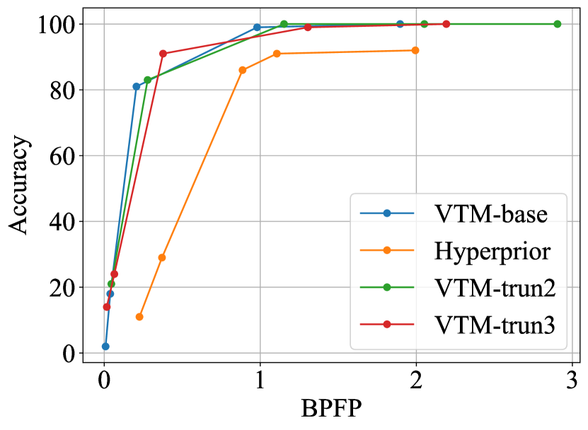
Semantic Segmentation

Depth Estimation

Common Sense Reasoning

Text-to-image Snythesis

$\lambda$-BPFP

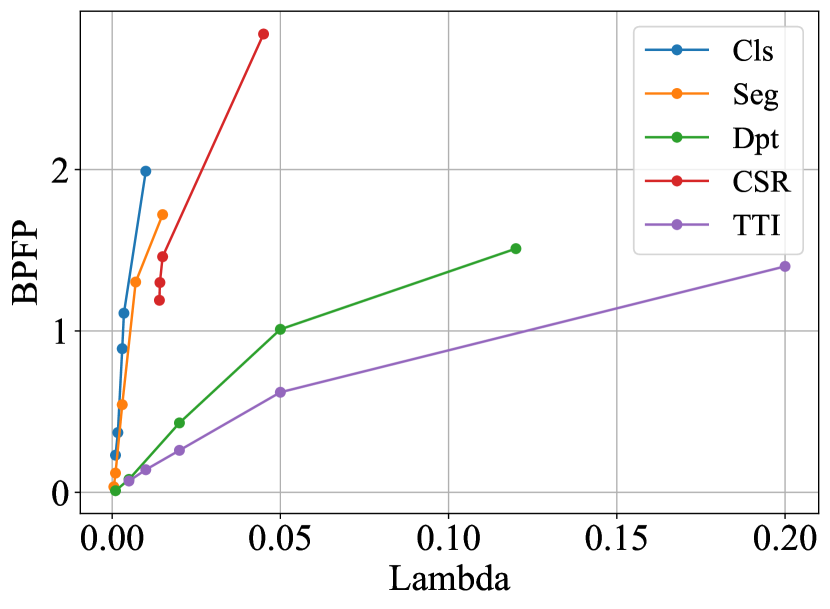
Figure 8: Visualization of rate-accuracy performance and $\lambda$-BPFP curves.

9 Baseline methods

9.1 Packing details

9.1.1 Semantic segmentation

In semantic segmentation, an image is pre-processed into multiple $518\times 518$ patches by crop and resize operations. These patches are fed into DINOv2, which produces features of shape $1370\times 1536$. In the proposed dataset, each image is pre-processed into 2 patches, resulting in features ($F_{Seg}$) with a shape of $2\times 1370\times 1536$. We reshape $F_{Seg}$ from $2\times 1370\times 1536$ into $2740\times 1536$ by vertically stacking them.

9.1.2 Depth estimation

In depth estimation, an image is first horizontally flipped. Both the original and flipped images are padded to dimensions that are multiples of 14 before being processed by DINOv2. For each image, DINOv2 generates $4\times 1611\times 1536$ embedding features at the split point $SP_{DM}$. Thus, the initial shape of $F_{Dpt}$ is $2\times 4\times 1611\times 1536$, where the two dimensions correspond to the original and flipped images. Packing $F_{Dpt}$ is performed in two steps. First, each $4\times 1611\times 1536$ feature is horizontally packed into a $1611\times 6144$ feature by concatenating the features along the width. Second, the two $1611\times 6144$ features (from the original and flipped images) are vertically stacked, resulting in a final feature shape of $3222\times 6144$.

9.1.3 Text-to-image synthesis

For text-to-image synthesis, the original feature $F_{TTI}$ has a shape of $16\times 128\times 128$, where 16 represents the number of channels. We divide the 16 channels into 4 subgroups. Within each subgroup, the $128\times 128$ features are horizontally concatenated to form a $128\times 512$ feature. Finally, the four $128\times 512$ features are vertically stacked to produce a final packed feature of size $512\times 512$.

9.2 Training details

9.2.1 Feature Pre-processing

Interestingly, we encountered the storage problem described in the main text during the training of feature coding models. For example, just 20000 original $F_{Dpt}$ features occupy 1474 GB of storage. As the need for additional training data grows, storage demands could escalate significantly. This often exceeds the resources available to researchers in academic institutions.

To address this issue, we crop the features into smaller dimensions to facilitate feature coding training. The specific cropping configurations are detailed in Table 9. However, it is important to note that vertical cropping is not effective for $F_{CSR}$. In our experiments, when $F_{CSR}$ is cropped into $64\times 512$, training becomes unstable, and the coding performance deteriorates significantly. We hypothesize that this limitation arises because $F_{CSR}$ is extracted from an LLM and involves only textual data.

It is worth emphasizing that while cropping is effective for feature coding training, this strategy is not applicable to large model training. For large models, it is unreasonable to crop portions of features to accelerate training, as downstream models typically require the entire semantic information. For example, cropping a $256\times 256$ patch from $F_{Dpt}$ would make it challenging to perform accurate depth estimation. Therefore, designing efficient feature coding methods remains crucial for reducing the storage burden in large model deployments.

Additionally, truncation and normalization operations are applied. The truncation regions listed in Table 4 are used. After truncation, all features are normalized into [0, 1].

9.2.2 Loss Function

In our experiments, we train models separately for each task. Across all tasks, the same loss function is employed. The loss function comprises two components: bitrate and feature MSE, defined as:

$$L=BPFP+\lambda\times||(F_{o}-\hat{F_{r}})||^{2}$$ (1)

where $\lambda$ is a scaling factor used to adjust the bitrate. A larger $\lambda$ corresponds to a higher bitrate.

9.2.3 Hyperparameter Setting

The number of training epochs, initial learning rate, and $\lambda$ values are provided in Table 9. The number of training epochs is determined based on the size of the training dataset. In our experiments, all training processes converge to a stable loss. Five different $\lambda$ values are used to achieve various bitrates. The $\lambda$ values are selected to align the bitrates with those achieved by the VTM baseline.

Image Classification

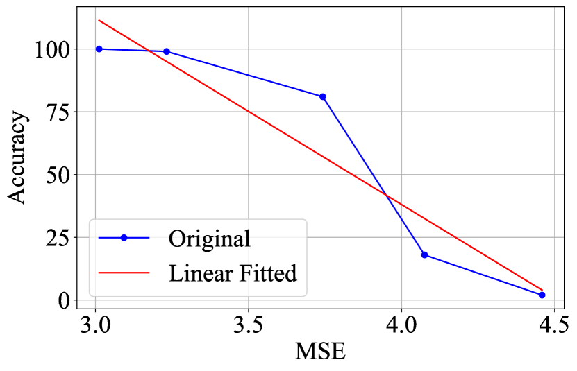
Image Classification

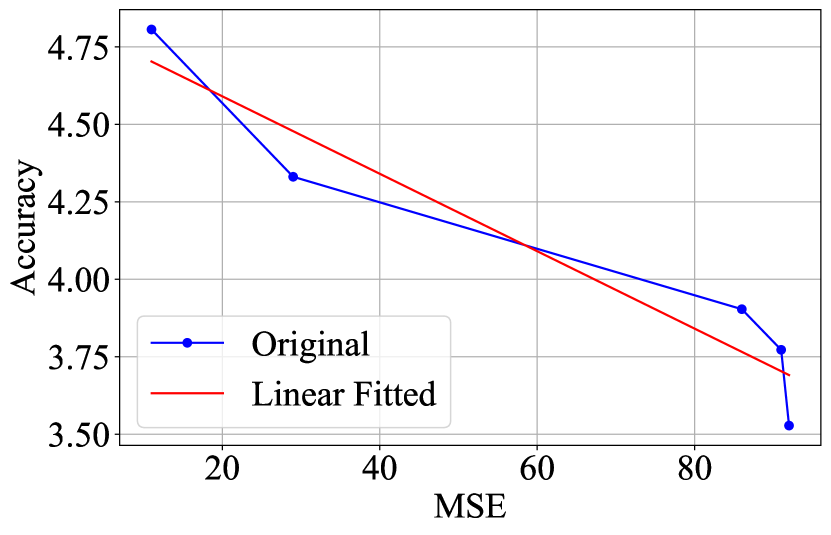
Semantic Segmentation

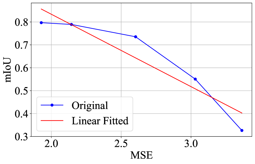
Semantic Segmentation

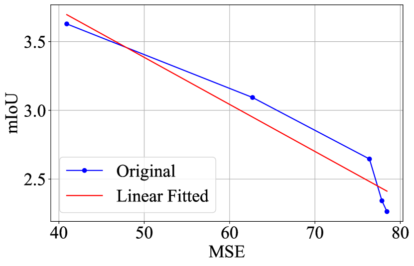
Depth Estimation

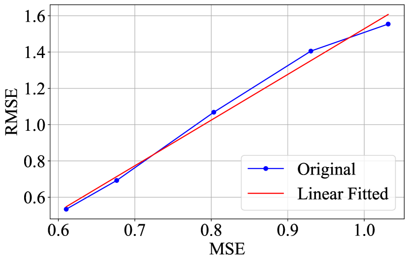
Depth Estimation

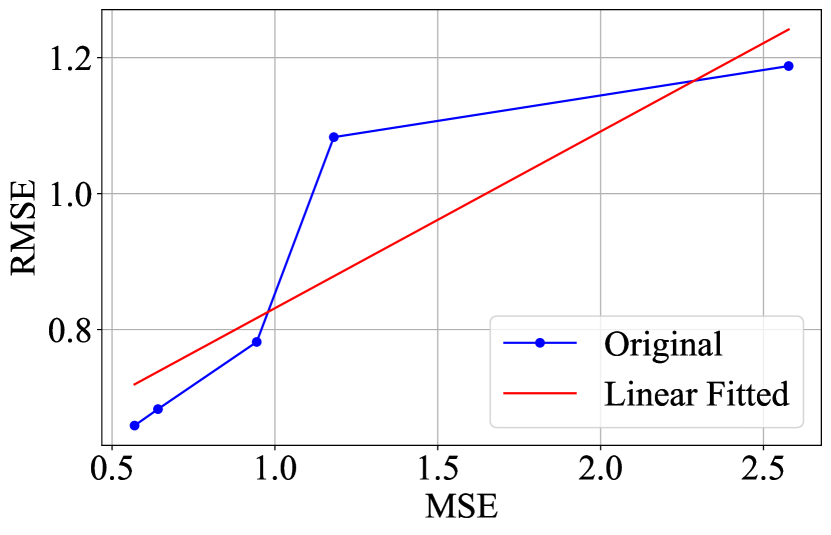
Common Sense Reasoning

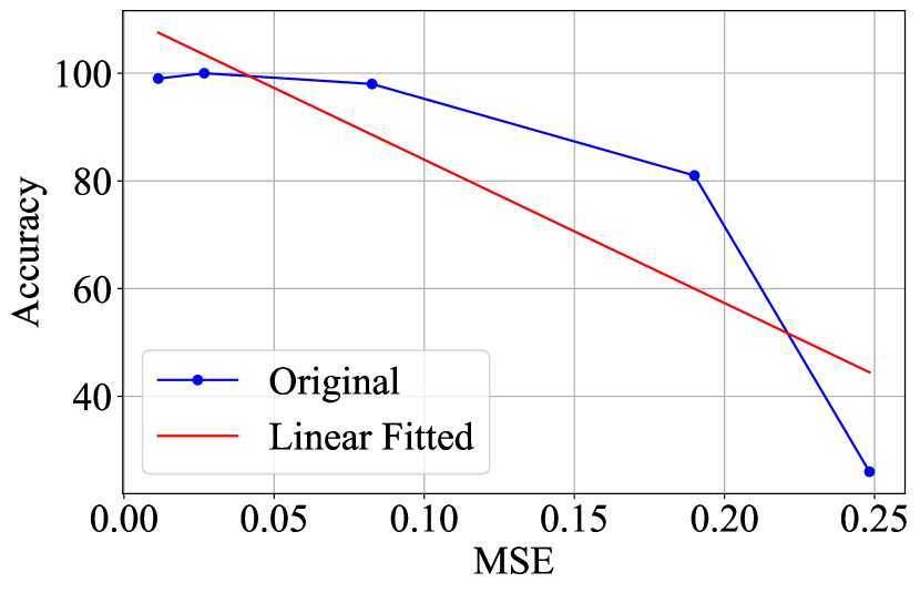
Common Sense Reasoning

Text-to-Image Synthesis

Text-to-Image Synthesis

Figure 9: Visualization of the linear relationship between feature MSE and task accuracy. Left: the VTM baseline. Right: the Hyperprior baseline.

	Image Classification			Semantic Segmentation
	BPFE	Accu.	Accu. Drop	BPFE	mIoU	mIoU Drop
VTM Baseline	1.90	100	0.00%	1.78	79.68	2.35%
	0.98	99	1.00%	0.90	78.91	3.30%
	0.21	81	19.00%	0.24	73.53	9.89%
	0.04	18	82.00%	0.04	55.05	32.54%
	0.01	2	98.00%	0.01	32.64	60.00%
Hyperprior Baseline (Trained on Classification)	1.99	92	8.00%	1.53	77.75	4.72%
	1.11	91	9.00%	0.88	75.22	7.82%
	0.89	86	14.00%	0.70	72.88	10.68%
	0.37	29	71.00%	0.24	62.23	23.73%
	0.23	11	89.00%	0.09	48.24	40.89%
Hyperprior Baseline (Trained on Segmentation)	2.41	97	3.00%	1.72	78.44	3.87%
	1.74	97	3.00%	1.30	77.85	4.59%
	0.87	86	14.00%	0.54	76.39	6.39%
	0.25	20	80.00%	0.12	62.69	23.17%
	0.09	1	99.00%	0.03	40.92	49.85%

Table 10: Rate-accuracy performance comparisons among different feature coding models.

10 Additional experimental results

10.1 Rate-accuracy analysis

We present the rate-accuracy curves in Fig. 8 to give a more straightforward comparison across different tasks. For semantic segmentation and depth estimation, the Hyperprior baseline achieves comparable coding performance to the VTM baseline. However, for the other three tasks, the performance is noticeably poorer. In the case of text-to-image synthesis, this is expected because $F_{TTI}$ shares a distribution similar to that of images and VTM has a higher coding performance in images than the Hyperprior codec. For image classification and common sense reasoning, improved truncation regions or quantization methods could potentially enhance coding performance. However, as feature pre-processing is not the focus of this paper, we leave this exploration to future studies.

For the VTM baseline, we conducted an ablation study on truncation regions. VTM-base, VTM-trun2, and VTM-trun3 correspond to the truncation regions specified in Table 4, the left one of Table 7, and the right one of Table 7, respectively. For depth estimation and common sense reasoning, the tested truncation regions significantly impact coding performance. As with feature pre-processing, the exploration of optimal truncation regions is deferred to future work.

10.2 Distortion-accuracy analysis

We visualize the distortion-accuracy curves in Fig. 9. The VTM baseline performs best in depth estimation, while the Hyperprior baseline achieves the highest linear correlation in text-to-image synthesis. These different behaviors highlight the distinct coding characteristics of the two methods. However, both baselines demonstrate the ineffectiveness of feature MSE as a metric for measuring semantic distortion.

$SP_{DM1},QP=42$

$SP_{DM1},\lambda=0.001$

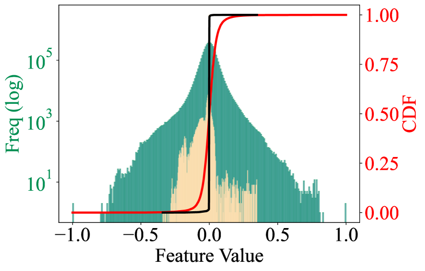
$SP_{DM2},QP=42$

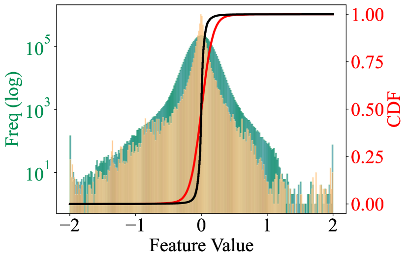
$SP_{DM2},\lambda=0.001$

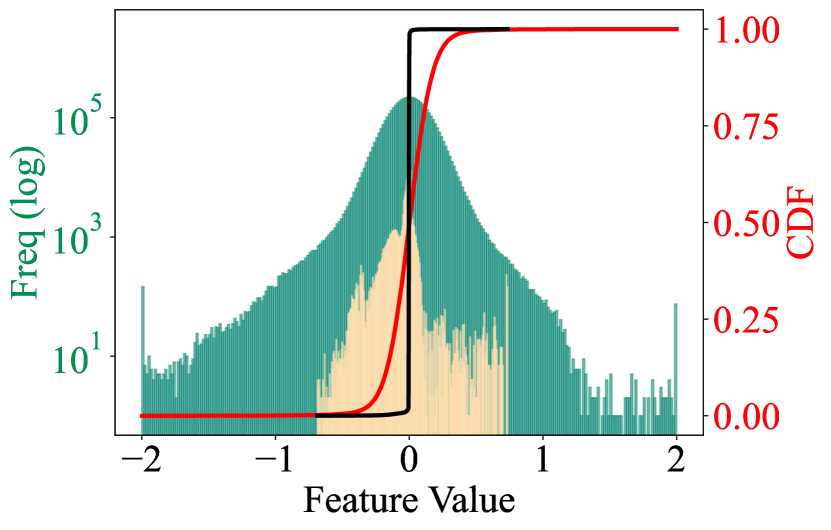
$SP_{DM3},QP=42$

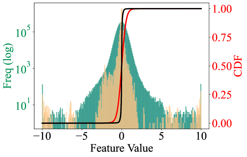
$SP_{DM3},\lambda=0.001$

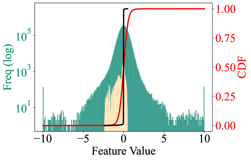
$SP_{DM4},QP=42$

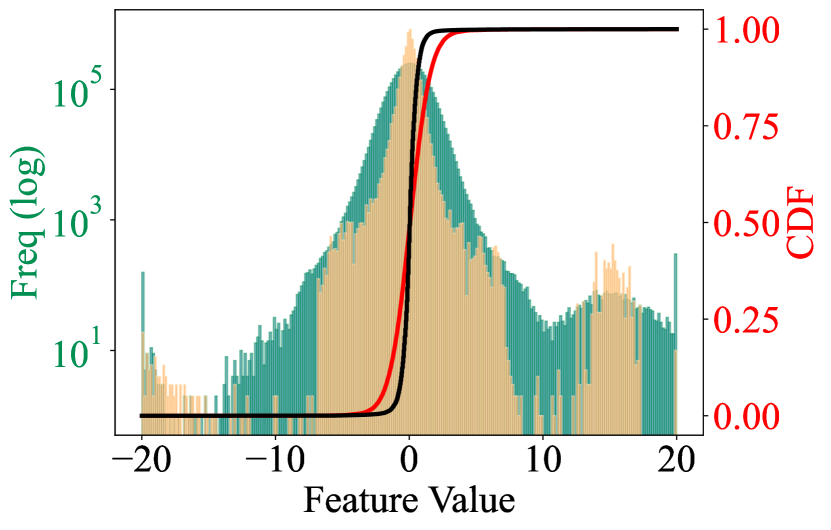
$SP_{DM4},\lambda=0.001$

$SP_{GS},QP=32$

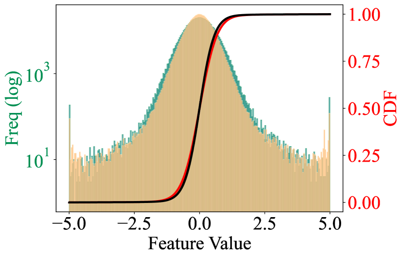
$SP_{GS},\lambda=0.01405$

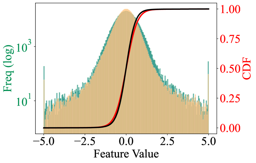
$SP_{H},QP=42$

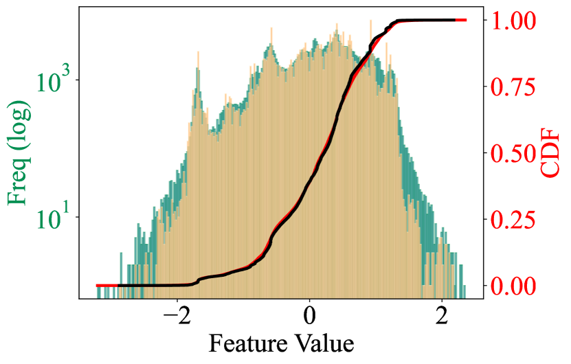
$SP_{H},\lambda=0.005$

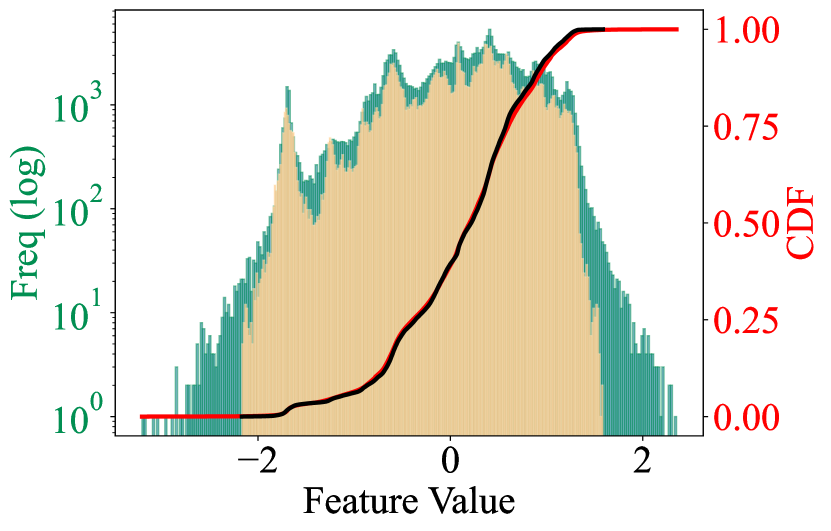
Figure 10: Frequency and CDF visualization of the original truncated and reconstructed features. Green and red are for the original truncated features. Yellow and black are for the reconstructed features. Left: the VTM baseline. Right: the Hyperprior baseline.

10.3 Exploration of generalization ability

We verify the generalization ability of the two baseline methods. First, we examine the $\lambda$-BPFP relationship and present the results in the bottom-right corner of Fig. 8. The analysis reveals that the same $\lambda$ produces different rate-distortion trade-offs across various tasks, indicating that features extracted from different tasks do not share similar coding properties.

To further investigate this, we select the two most similar tasks (image classification and semantic segmentation) based on their $\lambda$-BPFP curves and compare their rate-accuracy performance, as shown in Table 10. For the VTM baseline, although similar bitrates are achieved, the accuracy drop varies significantly at low bitrates. For the Hyperprior baseline, we encode $F_{Cls}$ and $F_{Seg}$ using two groups of models: models trained for image classification and models trained for semantic segmentation. Regardless of which group of models is used, different accuracy drops are observed.

These analyses indicate that the two proposed baselines lack generalization ability across various tasks. The generalization ability of feature coding methods across multiple tasks has received little attention in prior research. By presenting these results, we aim to draw more attention to this important research direction.

10.4 Feature distribution analysis

We visualize the distribution of reconstructed features in Fig. 10, comparing the two baseline methods at similar bitrates. For $SP_{DM}$, the Hyperprior baseline fails to reconstruct features within their original distribution range. The reconstructed features appear truncated during the feature coding process. We attribute this truncation to the inner quantization (rounding operation) in the Hyperprior codec, where the transformed latent variables are directly rounded to integers before entropy coding. In contrast, the VTM baseline quantizes original features into a broader distribution range of [0, 1023], effectively preventing the truncation phenomenon. A similar truncation phenomenon is observed for $SP_{H}$. For $SP_{GS}$, we visualize features encoded at a higher bitrate and observe that the truncation phenomenon disappears.

This truncation phenomenon highlights the incompatibility between features from large models and learned image coding methods. Two promising research directions emerge: (1) designing a new framework specifically tailored for feature coding, and (2) developing pre-processing techniques to adapt original features for compatibility with image coding methods.

References

- Ballé et al. [2018] Johannes Ballé, David C. Minnen, Saurabh Singh, Sung Jin Hwang, and Nick Johnston. Variational image compression with a scale hyperprior. ArXiv, abs/1802.01436, 2018.
- Bross et al. [2021] Benjamin Bross, Ye-Kui Wang, Yan Ye, Shan Liu, Jianle Chen, Gary J. Sullivan, and Jens-Rainer Ohm. Overview of the versatile video coding (VVC) standard and its applications. IEEE Transactions on Circuits and Systems for Video Technology, 31(10):3736–3764, 2021.
- Cai et al. [2022] Yangang Cai, Peiyin Xing, and Xuesong Gao. High efficient 3D convolution feature compression. IEEE Transactions on Circuits and Systems for Video Technology, pages 1–1, 2022.
- Chen et al. [2024a] Jingxue Chen, Hang Yan, Zhiyuan Liu, Min Zhang, Hu Xiong, and Shui Yu. When federated learning meets privacy-preserving computation. ACM Computing Surveys, 56(12):1–36, 2024a.
- Chen et al. [2024b] Qiaoxi Chen, Changsheng Gao, and Dong Liu. End-to-end learned scalable multilayer feature compression for machine vision tasks. In ICIP, pages 1781–1787, 2024b.
- Chen et al. [2020] Zhuo Chen, Kui Fan, Shiqi Wang, Lingyu Duan, Weisi Lin, and Alex Chichung Kot. Toward intelligent sensing: Intermediate deep feature compression. IEEE Transactions on Image Processing, 29:2230–2243, 2020.
- Choi and Bajić [2021] Hyomin Choi and Ivan V. Bajić. Latent-space scalability for multi-task collaborative intelligence. In ICIP, pages 3562–3566, 2021.
- Deng et al. [2009] Jia Deng, Wei Dong, Richard Socher, Li-Jia Li, Kai Li, and Li Fei-Fei. ImageNet: a large-scale hierarchical image database. In CVPR, pages 248–255, 2009.
- Docherty et al. [2024] Ronan Docherty, Antonis Vamvakeros, and Samuel J Cooper. Upsampling DINOv2 features for unsupervised vision tasks and weakly supervised materials segmentation. arXiv preprint arXiv:2410.19836, 2024.
- Duan et al. [2020] Lingyu Duan, Jiaying Liu, Wenhan Yang, Tiejun Huang, and Wen Gao. Video coding for machines: A paradigm of collaborative compression and intelligent analytics. IEEE Transactions on Image Processing, 29:8680–8695, 2020.
- Dubey et al. [2024] Abhimanyu Dubey, Abhinav Jauhri, Abhinav Pandey, Abhishek Kadian, Ahmad Al-Dahle, Aiesha Letman, Akhil Mathur, Alan Schelten, Amy Yang, Angela Fan, et al. The Llama 3 herd of models. arXiv preprint arXiv:2407.21783, 2024.
- Esser et al. [2024] Patrick Esser, Sumith Kulal, Andreas Blattmann, Rahim Entezari, Jonas Müller, Harry Saini, Yam Levi, Dominik Lorenz, Axel Sauer, Frederic Boesel, et al. Scaling rectified flow transformers for high-resolution image synthesis. In ICML, 2024.
- Feng et al. [2022] Ruoyu Feng, Xin Jin, Zongyu Guo, Runsen Feng, Yixin Gao, Tianyu He, Zhizheng Zhang, Simeng Sun, and Zhibo Chen. Image coding for machines with omnipotent feature learning. In ECCV, pages 510–528. Springer, 2022.
- Friha et al. [2024] Othmane Friha, Mohamed Amine Ferrag, Burak Kantarci, Burak Cakmak, Arda Ozgun, and Nassira Ghoualmi-Zine. LLM-based edge intelligence: A comprehensive survey on architectures, applications, security and trustworthiness. IEEE Open Journal of the Communications Society, 5:5799–5856, 2024.
- Gao et al. [2023] Changsheng Gao, Dong Liu, Li Li, and Feng Wu. Towards task-generic image compression: A study of semantics-oriented metrics. IEEE Transactions on Multimedia, 25:721–735, 2023.
- Gao et al. [2024a] Changsheng Gao, Yiheng Jiang, Li Li, Dong Liu, and Feng Wu. Dmofc: Discrimination metric-optimized feature compression. In PCS, pages 1–5, 2024a.
- Gao et al. [2024b] Changsheng Gao, Yiheng Jiang, Siqi Wu, Yifan Ma, Li Li, and Dong Liu. Imofc: Identity-level metric optimized feature compression for identification tasks. IEEE Transactions on Circuits and Systems for Video Technology, pages 1–1, 2024b.
- Kaddour et al. [2023] Jean Kaddour, Joshua Harris, Maximilian Mozes, Herbie Bradley, Roberta Raileanu, and Robert McHardy. Challenges and applications of large language models. arXiv preprint arXiv:2307.10169, 2023.
- Kim et al. [2023] Yeongwoong Kim, Hyewon Jeong, Janghyun Yu, Younhee Kim, Jooyoung Lee, Se Yoon Jeong, and Hui Yong Kim. End-to-end learnable multi-scale feature compression for VCM. IEEE Transactions on Circuits and Systems for Video Technology, pages 1–1, 2023.
- Kirillov et al. [2023] Alexander Kirillov, Eric Mintun, Nikhila Ravi, Hanzi Mao, Chloe Rolland, Laura Gustafson, Tete Xiao, Spencer Whitehead, Alexander C Berg, Wan-Yen Lo, et al. Segment anything. In Proceedings of the IEEE/CVF International Conference on Computer Vision, pages 4015–4026, 2023.
- Lee et al. [2019] Jin Han Lee, Myung-Kyu Han, Dong Wook Ko, and Il Hong Suh. From big to small: Multi-scale local planar guidance for monocular depth estimation. arXiv preprint arXiv:1907.10326, 2019.
- Lepikhin et al. [2020] Dmitry Lepikhin, HyoukJoong Lee, Yuanzhong Xu, Dehao Chen, Orhan Firat, Yanping Huang, Maxim Krikun, Noam Shazeer, and Zhifeng Chen. GShard: Scaling giant models with conditional computation and automatic sharding. arXiv preprint arXiv:2006.16668, 2020.
- Li et al. [2023] Shibao Li, Chenxu Ma, Yunwu Zhang, Longfei Li, Chengzhi Wang, Xuerong Cui, and Jianhang Liu. Attention-based variable-size feature compression module for edge inference. The Journal of Supercomputing, 2023.
- Liu et al. [2023] Tie Liu, Mai Xu, Shengxi Li, Chaoran Chen, Li Yang, and Zhuoyi Lv. Learnt mutual feature compression for machine vision. In ICASSP, pages 1–5, 2023.
- Lu et al. [2024] Guo Lu, Xingtong Ge, Tianxiong Zhong, Qiang Hu, and Jing Geng. Preprocessing enhanced image compression for machine vision. IEEE Transactions on Circuits and Systems for Video Technology, pages 1–1, 2024.
- Lyu et al. [2024] Lingjuan Lyu, Han Yu, Xingjun Ma, Chen Chen, Lichao Sun, Jun Zhao, Qiang Yang, and Philip S. Yu. Privacy and robustness in federated learning: Attacks and defenses. IEEE Transactions on Neural Networks and Learning Systems, 35(7):8726–8746, 2024.
- Misra et al. [2022] Kiran Misra, Tianying Ji, Andrew Segall, and Frank Bossen. Video feature compression for machine tasks. In ICME, pages 1–6, 2022.
- Oquab et al. [2023] Maxime Oquab, Timothée Darcet, Théo Moutakanni, Huy Vo, Marc Szafraniec, Vasil Khalidov, Pierre Fernandez, Daniel Haziza, Francisco Massa, Alaaeldin El-Nouby, et al. DINOv2: Learning robust visual features without supervision. arXiv preprint arXiv:2304.07193, 2023.
- Radford et al. [2021] Alec Radford, Jong Wook Kim, Chris Hallacy, Aditya Ramesh, Gabriel Goh, Sandhini Agarwal, Girish Sastry, Amanda Askell, Pamela Mishkin, Jack Clark, et al. Learning transferable visual models from natural language supervision. In ICML, pages 8748–8763. PMLR, 2021.
- Sun et al. [2023] Quan Sun, Yuxin Fang, Ledell Wu, Xinlong Wang, and Yue Cao. Eva-CLIP: improved training techniques for clip at scale. arXiv preprint arXiv:2303.15389, 2023.
- Suzuki et al. [2022] Satoshi Suzuki, Shoichiro Takeda, Motohiro Takagi, Ryuichi Tanida, Hideaki Kimata, and Hayaru Shouno. Deep feature compression using spatio-temporal arrangement toward collaborative intelligent world. IEEE Transactions on Circuits and Systems for Video Technology, 32(6):3934–3946, 2022.
- Tian et al. [2022] Yuanyishu Tian, Yao Wan, Lingjuan Lyu, Dezhong Yao, Hai Jin, and Lichao Sun. FedBERT: when federated learning meets pre-training. ACM Transactions on Intelligent Systems and Technology, 13(4):1–26, 2022.
- Tian et al. [2023] Yuan Tian, Guo Lu, Guangtao Zhai, and Zhiyong Gao. Non-semantics suppressed mask learning for unsupervised video semantic compression. In ICCV, pages 13564–13576, 2023.
- Tian et al. [2024] Yuan Tian, Guo Lu, and Guangtao Zhai. SMC++: masked learning of unsupervised video semantic compression. arXiv preprint arXiv:2406.04765, 2024.
- Tian et al. [2025] Yuan Tian, Guo Lu, and Guangtao Zhai. Free-VSC: free semantics from visual foundation models for unsupervised video semantic compression. In ECCV, pages 163–183, 2025.
- Touvron et al. [2023] Hugo Touvron, Thibaut Lavril, Gautier Izacard, Xavier Martinet, Marie-Anne Lachaux, Timothée Lacroix, Baptiste Rozière, Naman Goyal, Eric Hambro, Faisal Azhar, et al. Llama: Open and efficient foundation language models. arXiv preprint arXiv:2302.13971, 2023.
- Vepakomma et al. [2018] Praneeth Vepakomma, Otkrist Gupta, Tristan Swedish, and Ramesh Raskar. Split learning for health: Distributed deep learning without sharing raw patient data. arXiv preprint arXiv:1812.00564, 2018.
- Wang et al. [2022] Shurun Wang, Shiqi Wang, Wenhan Yang, Xinfeng Zhang, Shanshe Wang, Siwei Ma, and Wen Gao. Towards analysis-friendly face representation with scalable feature and texture compression. IEEE Transactions on Multimedia, 24:3169–3181, 2022.
- Wu et al. [2024] Shengqiong Wu, Hao Fei, Leigang Qu, Wei Ji, and Tat-Seng Chua. NExT-GPT: Any-to-any multimodal LLM. In ICML, pages 53366–53397, 2024.
- Yan et al. [2024] Biwei Yan, Kun Li, Minghui Xu, Yueyan Dong, Yue Zhang, Zhaochun Ren, and Xiuzhen Cheng. On protecting the data privacy of large language models (LLMs): A survey. arXiv preprint arXiv:2403.05156, 2024.
- Yan et al. [2021] Ning Yan, Changsheng Gao, Dong Liu, Houqiang Li, Li Li, and Feng Wu. SSSIC: Semantics-to-signal scalable image coding with learned structural representations. IEEE Transactions on Image Processing, 30:8939–8954, 2021.
- Yang et al. [2024] Wenhan Yang, Haofeng Huang, Yueyu Hu, Ling-Yu Duan, and Jiaying Liu. Video coding for machines: Compact visual representation compression for intelligent collaborative analytics. IEEE Transactions on Pattern Analysis and Machine Intelligence, pages 1–18, 2024.
- Ye et al. [2024] Rui Ye, Wenhao Wang, Jingyi Chai, Dihan Li, Zexi Li, Yinda Xu, Yaxin Du, Yanfeng Wang, and Siheng Chen. OpenFedLLM: Training large language models on decentralized private data via federated learning. In ACM SIGKDD, pages 6137–6147, 2024.
- Zhang et al. [2024] Xu Zhang, Peiyao Guo, Ming Lu, and Zhan Ma. All-in-one image coding for joint human-machine vision with multi-path aggregation. arXiv preprint arXiv:2409.19660, 2024.
- Zhang et al. [2021] Zhicong Zhang, Mengyang Wang, Mengyao Ma, Jiahui Li, and Xiaopeng Fan. MSFC: Deep feature compression in multi-task network. In ICME, pages 1–6, 2021.
- Zheng et al. [2024] JiaYing Zheng, HaiNan Zhang, LingXiang Wang, WangJie Qiu, HongWei Zheng, and ZhiMing Zheng. Safely learning with private data: A federated learning framework for large language model. arXiv preprint arXiv:2406.14898, 2024.