Sector-angle-periodic generalization of quad-mesh rigid origami and its convergence to smooth surfaces

Abstract

A quad-mesh rigid origami is a continuously deformable panel-hinge structure where rigid zero-thickness quad panels are connected by rotational hinges in the combinatorics of a grid. This article introduces two new families of generalized sector-angle-periodic quad-mesh rigid origami stitched from proportional and equimodular couplings, expanding beyond commonly known variations such as V-hedra (discrete Voss surface/eggbox pattern), anti-V-hedra (flat-foldable pattern) and T-hedra (trapezoidal pattern). We conjecture that as the mesh is refined to infinity, these quad-mesh rigid origami converges to special ruled surfaces in the limit, supported by multiple lines of evidence. Additionally, we discuss the convergence of tangent planes, metric-related, and curvature-related properties.

1 Introduction

A quad-mesh rigid origami is a structure composed of rigid, flat, and zero-thickness quadrilateral panels jointed by rotational hinges in a grid-like connectivity, which admits a continuous isometric deformation without deforming the panels. This deformation is also called a flex, flexion or folding motion in different literatures. We show the most famous quad-mesh rigid origami – the Miura ori (Miura, 1985), in Figure 1(a). In the origami community, the primary focus is on developable origami, which means the sum of sector angles around every interior vertex is $2\pi$. Upon this condition, the discrete Gaussian curvature at every interior vertex would be zero (details provided at the end of Section D of the Supplementary Material). While in our setup, the sum of sector angles at every interior vertex is not necessarily $2\pi$, which means our discussion includes but is not restricted to developable origami. The most commonly applied quad-mesh rigid origami are (anti-)V-hedra and T-hedra, as depicted in Figure 1(b)–(f). In this article, we focus on more generalized quad-mesh rigid origami that extend beyond (anti-)V-hedra and T-hedra, namely, those stitched from proportional and equimodular couplings. The mathematical description of these terms, originating from Izmestiev (2017), are provided in Sections K and L, respectively, of the Supplementary Material. To clarify the distinctions among these different types of quad-mesh rigid origami, we begin with a brief overview of (anti-)V-hedra and (anti-)T-hedra.

(Anti-)V-hedra and (anti-)T-hedra

A V-hedron (Figure 1(b) and 1(c)) refers to a non-developable quad-mesh rigid origami where opposite sector angles are equal at every interior vertex ($\alpha=\gamma,~{}\beta=\delta$ if the sector angles at a vertex are denoted by $\alpha,~{}\beta,~{}\gamma,~{}\delta$). It has a special state where the folding angle at every vertex is $\{\pm\pi,~{}0,~{}\pm\pi,~{}0\}$ (in a cyclic order), which can be folded to another special state where the folding angle at every vertex is $\{0,~{}\pm\pi,~{}0,~{}\pm\pi\}$ (in the same cyclic order). The name V-hedron is from the early research on Voss surface (Voss, 1888) and discrete Voss surface (Sauer and Graf, 1931), which is also called an eggbox pattern in the origami community (Tachi, 2010). An anti-V-hedron (Figure 1(d)) is a developable quad-mesh rigid origami where opposite sector angles are supplementary to $\pi$ at every interior vertex ($\alpha+\gamma=\pi,~{}\beta+\delta=\pi$). This pattern is widely recognized as a developable, flexible (also called rigid-foldable in different literatures) and flat-foldable quad-mesh origami (Tachi, 2009). It has a planar state where all the folding angles are zero, which can be folded to another flatly-folded state where the folding angle at every vertex is $\pm\pi$.

In He and Guest (2020) we showed that switching a strip — changing the sector angles on a row or column of quadrilateral panels to their supplements with respect to $\pi$ — maps a quad-mesh rigid origami to another quad-mesh rigid origami and preserves the flexibility. A V-hedron becomes an anti-V-hedron after switching all the strips, and becomes a hybrid V-hedron (also discussed in Tachi (2010)) if only switching some strips. Details on the flexibility of quad-mesh rigid origami and operations generating quad-mesh rigid origami from an existing one are provided in Section H of the Supplementary Material.

A T-hedron (Figure 1(e) and (f)) refers to a quad-mesh rigid origami whose vertices are orthodiagonal ($\cos\alpha\cos\gamma=\cos\beta\cos\delta$) and every two vertices form an involutive coupling. These terminologies are special geometric requirements on the sector angles (Izmestiev, 2017, Section 3.1). A T-hedron can be developable or non-developable. The name T-hedron is from Sauer and Graf (1931). An anti-T-hedron refers to a quad-mesh rigid origami whose vertices are orthodiagonal and every two vertices form an anti-involutive coupling. The $3\times 3$ building block for an anti-T-hedron was studied in Erofeev and Ivanov (2020), yet there has not been reported progress on how to stitch it to form a large pattern.

A more comprehensive introduction of (anti-)V-hedra and T-hedra is provided in Sections I and J of the Supplementary Material.

Surface approximation

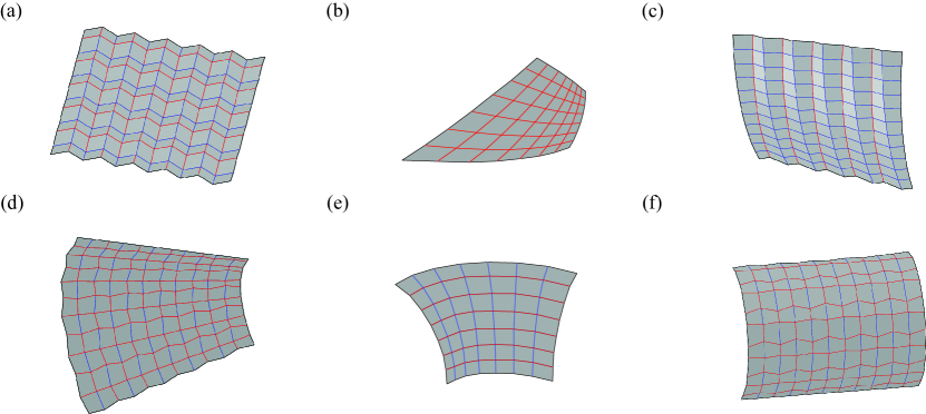
Figure 1: A brief gallery of common quad-mesh rigid origami, including (a) the Miura-ori (Miura, 1985); (b) a non-developable V-hedron (Sauer, 1970); (c) another non-developable V-hedron; (d) a developable anti-V-hedron; (e) a non-developable T-hedron (Izmestiev et al., 2024b) ; and (f) a developable T-hedron. Mountain creases are coloured red and valley creases are coloured blue.

In addition to the variety of quad-mesh rigid origami, there has been a continuous effort within the origami research community to explore which surfaces a quad-mesh rigid origami can approximate. We are further motivated to explore how closely a quad-mesh rigid origami can approximate a smooth surface as the mesh is refined. In other words, for a series of quad-mesh rigid origami following a construction method that allows arbitrary mesh refinement, we aim to investigate the convergence toward a smooth surface in terms of Euclidean distance (detailed in Section G of the Supplementary Material). Hereafter, ‘distance’ refers to Euclidean distance throughout the article.

The first level of surface approximation happens when a series of quad-mesh rigid origami converge to a smooth surface in distance, and they represent the discrete and smooth forms of the same coordinate net. Consequently, as the mesh is refined, their tangent planes, metric-related and curvature-related properties can become arbitrarily close. Furthermore, the single-degree-of-freedom folding motion of this series of quad-mesh rigid origami converges to the flex of the limit smooth surface. Certain V-hedra and T-hedra reach this level of approximation, with the resulting smooth surfaces referred to as V-surfaces (Bianchi, 1890; Sauer, 1970; Izmestiev et al., 2024a) in Figure 1(b) and T-surfaces (Izmestiev et al., 2024b) in Figure 1(e). Due to this unique relationship, we refer to them as discrete and smooth analogues of one another. Related information in (discrete) differential geometry is provided in Part I of the Supplementary Material.

The next level of surface approximation involves convergence only in terms of distance, without guaranteeing the convergence of tangent planes or properties related to metric and curvature. A limit smooth surface can be reached with a series of quad-mesh rigid origami, while there is no guarantee about the convergence of their motion. Some other V-hedra and T-hedra fall into this category, as shown in Figure 1(a), (c), (d), and (f). Examples include the Miura-ori (Miura, 1985) and revolutionary Miura-ori (Song et al., 2017; Hu et al., 2019). Although we can design this pattern to be close to a plane or a surface of revolution, the origami structure deviates further from these target surfaces as it is folded flat. A common feature for them is they have a ‘zig-zag’ mode — we will explain this further in the Discussion section below.

The third level of surface approximation is frequently employed in origami-based engineering design, such as pavilions, shelters and shells. It would be geometrically sufficient if the origami structure can exhibit desired curvature with limited number of grids. Numerous publications have explored such inverse design employing V-hedra, anti-V-hedra or T-hedra to construct three-dimensional structures. Notably, the number of free variables for an (anti-)V-hedron increases linearly with respected to the number of grids, hence there is sufficient space for shape optimization. The inputs for these inverse design include perturbation from an existing pattern (Tachi, 2010); ‘curved creases’ (Jiang et al., 2019); an array of folding angles and crease lengths of boundary polylines (Lang and Howell, 2018); a target surface (Dang et al., 2022); the discrete normal field/Gauss map (Montagne et al., 2022); and control polylines or vertices (Kilian et al., 2024). T-hedra have less free variables and are less frequently applied yet, but showed great promise for highly accurate approximation of certain surfaces. The inputs include boundary/control polylines (He and Guest, 2018; Sharifmoghaddam et al., 2020). Additionally, He and Guest (2018) showed that it is possible to ‘stitch’ anti-V-hedra and T-hedra to construct developable structures with the ‘self-locking’ property – the motion halts at desired configuration due to the clash of panels.

Result and method

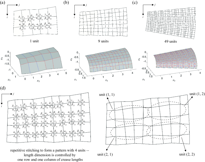
Figure 2: Repetitive stitching of rectangular units to generate a quad-mesh rigid origami. (a) shows a unit and our labelling of sector angles. (b) and (c) show the approximation to a smooth surface from refining the mesh. (d) illustrates the stitching process, where sector angles from one unit are repeated and stitched together to form the new pattern with 4 units. One row and one column of crease lengths can be adjusted. This example was once shown in He et al. (2024), where our focus is to introduce new patterns with the motion-guarantee property — the existence of a non-trivial state guarantees a motion.

In this section, we introduce construction methods that allow infinite mesh refinement for two newly identified families of quad-mesh rigid origami, which are stitched from proportional and equimodular couplings, named after their distinct geometrical characteristics in Izmestiev (2017). It is widely accepted that a large quad-mesh rigid origami is flexible if and only if all its $3\times 3$ quadrilaterals (Kokotsakis quadrilaterals) are flexible (Schief et al., 2008). Thus, by utilizing the classification of flexible Kokotsakis quadrilaterals provided in Izmestiev (2017), it is possible to construct a large quad-mesh rigid origami by ‘stitching’ together these $3\times 3$ building blocks. However, Izmestiev (2017) describes each type of flexible Kokotsakis quadrilateral by a system of highly nonlinear equations on the sector angles, which is obtained from the calculation conducted in the complexified configuration space. The above limitation necessitates examining: 1) the existence of real solutions to these systems; and 2) the existence of an actual folding motion in $\mathbb{R}^{3}$. Additionally, to support mesh refinement to infinity, 3) the stitching method should be ‘infinitely extendable’, rather than restricted in a finite grid. We select two families satisfying requirements 1) to 3) from He and Guest (2020), and, to explore the form-finding capability of them, we apply an additional periodic condition to the sector angles, as described below.

The construction method is named repetitive stitching of rectangular units. Figure 2(a) shows a $3\times 5$ unit with 8 interior vertices and 32 sector angles. The progression from Figure 2(a) to (c) demonstrates how the construction approximates a smooth surface through mesh refinement. Figure 2(d) illustrates the repetitive stitching process, where sector angles from one unit are replicated and stitched together to create the new pattern. The crease lengths of a single row and column can be adjusted to fully determine the shape of the entire pattern.

In this example, the sector angles $\alpha_{ij},~{}\beta_{ij},~{}\gamma_{ij},~{}\delta_{ij}$, $i,~{}j\in\mathbb{Z}_{+},~{}i\leq 2,~{}j\leq 4$ meet the constraints below, which ensures the flexibility of the entire pattern. There are 30 constraints for 32 sector angles, hence roughly speaking, allowing two independent input sector angles. Details on the derivation of these constraints are provided in Sections H and K of the Supplementary Material.

Vertex type condition (half are anti-isogram/flat-foldable vertices, half are anti-deltoid II/straight-line vertices):

$$\begin{dcases}\gamma_{11}=\pi-\alpha_{11},~{}\delta_{11}=\pi-\beta_{11},~{}\gamma_{12}=\pi-\alpha_{12},~{}\delta_{12}=\pi-\beta_{12}\\ \gamma_{13}=\pi-\alpha_{13},~{}\delta_{13}=\pi-\beta_{13},~{}\gamma_{14}=\pi-\alpha_{14},~{}\delta_{14}=\pi-\beta_{14}\\ \gamma_{21}=\pi-\beta_{21},~{}\delta_{21}=\pi-\alpha_{21},~{}\gamma_{22}=\pi-\beta_{22},~{}\delta_{22}=\pi-\alpha_{22}\\ \gamma_{23}=\pi-\beta_{23},~{}\delta_{23}=\pi-\alpha_{23},~{}\gamma_{24}=\pi-\beta_{24},~{}\delta_{24}=\pi-\alpha_{24}\\ \end{dcases}$$

Planarity condition of quad panels considering the periodicity of sector angles:

$$\begin{dcases}\beta_{11}+\beta_{21}+\beta_{12}+\beta_{12}=2\pi,~{}\gamma_{11}+\gamma_{21}+\gamma_{12}+\gamma_{12}=2\pi\\ \delta_{12}+\delta_{22}+\delta_{13}+\delta_{23}=2\pi,~{}\alpha_{12}+\alpha_{22}+\alpha_{13}+\alpha_{23}=2\pi\\ \beta_{13}+\beta_{23}+\beta_{14}+\beta_{14}=2\pi,~{}\gamma_{13}+\gamma_{23}+\gamma_{14}+\gamma_{14}=2\pi\\ \delta_{14}+\delta_{24}+\delta_{11}+\delta_{21}=2\pi,~{}\alpha_{14}+\alpha_{24}+\alpha_{11}+\alpha_{21}=2\pi\\ \end{dcases}$$

Condition for being proportional units:

$$\begin{dcases}\dfrac{\sin\alpha_{21}}{\sin\beta_{21}}=\dfrac{\sin\alpha_{22}}{\sin\beta_{22}}\\ \dfrac{\sin\alpha_{22}}{\sin\beta_{22}}=\dfrac{\sin\alpha_{23}}{\sin\beta_{23}}\\ \dfrac{\sin\alpha_{23}}{\sin\beta_{23}}=\dfrac{\sin\alpha_{24}}{\sin\beta_{24}}\\ \end{dcases}$$

Condition on equal ratio for proportional units:

$$\begin{dcases}\begin{split}&\dfrac{\sin\dfrac{\beta_{11}-\gamma_{11}}{2}\sin\dfrac{\beta_{12}+\gamma_{12}}{2}}{\sin\dfrac{\beta_{11}+\gamma_{11}}{2}\sin\dfrac{\beta_{12}-\gamma_{12}}{2}}=\\ &\mathrm{sign}\left(\dfrac{\pi-\beta_{21}-\alpha_{21}}{\pi-\beta_{22}-\alpha_{22}}\right)\sqrt{\dfrac{\sin(\beta_{21}+\alpha_{21})\sin(\beta_{22}-\alpha_{22})}{\sin(\beta_{21}-\alpha_{21})\sin(\beta_{22}+\alpha_{22})}}\end{split}\\ \begin{split}&\dfrac{\sin\dfrac{\beta_{12}-\gamma_{12}}{2}\sin\dfrac{\beta_{13}+\gamma_{13}}{2}}{\sin\dfrac{\beta_{12}+\gamma_{12}}{2}\sin\dfrac{\beta_{13}-\gamma_{13}}{2}}=\\ &\mathrm{sign}\left(\dfrac{\pi-\beta_{22}-\alpha_{22}}{\pi-\beta_{23}-\alpha_{23}}\right)\sqrt{\dfrac{\sin(\beta_{22}+\alpha_{22})\sin(\beta_{23}-\alpha_{23})}{\sin(\beta_{22}-\alpha_{22})\sin(\beta_{23}+\alpha_{23})}}\end{split}\\ \begin{split}&\dfrac{\sin\dfrac{\beta_{13}-\gamma_{13}}{2}\sin\dfrac{\beta_{14}+\gamma_{14}}{2}}{\sin\dfrac{\beta_{13}+\gamma_{13}}{2}\sin\dfrac{\beta_{14}-\gamma_{14}}{2}}=\\ &\mathrm{sign}\left(\dfrac{\pi-\beta_{23}-\alpha_{23}}{\pi-\beta_{24}-\alpha_{24}}\right)\sqrt{\dfrac{\sin(\beta_{23}+\alpha_{23})\sin(\beta_{24}-\alpha_{24})}{\sin(\beta_{23}-\alpha_{23})\sin(\beta_{24}+\alpha_{24})}}\end{split}\end{dcases}$$

Note that the two equations below will be implied from the above conditions, which also contributes to the flexibility condition of the entire quad-mesh rigid origami:

$$\begin{dcases}\dfrac{\sin\alpha_{24}}{\sin\beta_{24}}=\dfrac{\sin\alpha_{21}}{\sin\beta_{21}}\\ \begin{split}&\dfrac{\sin\dfrac{\beta_{14}-\gamma_{14}}{2}\sin\dfrac{\beta_{11}+\gamma_{11}}{2}}{\sin\dfrac{\beta_{14}+\gamma_{14}}{2}\sin\dfrac{\beta_{11}-\gamma_{11}}{2}}=\\ &\mathrm{sign}\left(\dfrac{\pi-\beta_{24}-\alpha_{24}}{\pi-\beta_{21}-\alpha_{21}}\right)\sqrt{\dfrac{\sin(\beta_{24}+\alpha_{24})\sin(\beta_{21}-\alpha_{21})}{\sin(\beta_{24}-\alpha_{24})\sin(\beta_{21}+\alpha_{21})}}\\ \end{split}\end{dcases}$$

It turns out that one can create a large library of quad-mesh rigid origami using repetitive stitching of rectangular units formed from proportional and equimodular couplings, with varying vertex types, input sector angles, and crease length distributions. Figure 3 presents six additional examples with both uniform and quadratic input crease length distribution, showcasing the effect of varying input crease lengths. The sector angles of these examples were solved numerically and validated with a high degree of accuracy (error less than 1e-15). All relevant details are presented in Sections K, L and M of the Supplementary Material. The accompanying MATLAB application (He, 2024) includes all data and serves as a convenient tool for parametric design, mesh refinement, and 3D visualization of folding motion.

We conjecture that a special ruled surface $x(u_{1},~{}u_{2})$ in the form below can be approximated (at the second level of surface approximation, as introduced on page 4) by a series of quad-mesh rigid origami using repetitive stitching of rectangular units:

$$\begin{gathered}x(u_{1},~{}u_{2})=\Gamma(u_{2})+u_{1}\Phi(u_{2}),~{}~{}u_{1},~{}u_{2}\in\mathbb{R},~{}~{}x\in\mathbb{R}^{3}\\ \Gamma(u_{2})=\Gamma(0)+\int\limits_{v=0}^{u_{2}}f(v)\begin{bmatrix}-a\sin v\\ a\cos v\\ b\end{bmatrix}\mathop{}\!\mathrm{d}v,~{}a>0,~{}b\in\mathbb{R}\\ f(u_{2})=\dfrac{\left\|\dfrac{\mathop{}\!\mathrm{d}\Gamma}{\mathop{}\!\mathrm{d}u_{2}}(u_{2})\right\|}{\left\|\dfrac{\mathop{}\!\mathrm{d}\Gamma}{\mathop{}\!\mathrm{d}u_{2}}(0)\right\|}\\ \Phi(u_{2})\in\mathbb{R}^{3},~{}||\Phi(u_{2})||\equiv 1\\ \dfrac{\dfrac{\mathop{}\!\mathrm{d}\Gamma}{\mathop{}\!\mathrm{d}u_{2}}\cdot\Phi}{f\sqrt{a^{2}+b^{2}}}=\mathrm{Const}\in[0,1)\end{gathered}$$ (1)

where $f(u_{2})$ is a known input crease lengths distribution function, $\Gamma(u_{2})$ is the directrix and $\Phi(u_{2})$ is the direction of rulings. Evidence supporting this conjecture is provided in Section N of the Supplementary Material. Eq. (1) can be used to calculate the apparent curvature of the origami structure and to develop optimal inverse design algorithms.

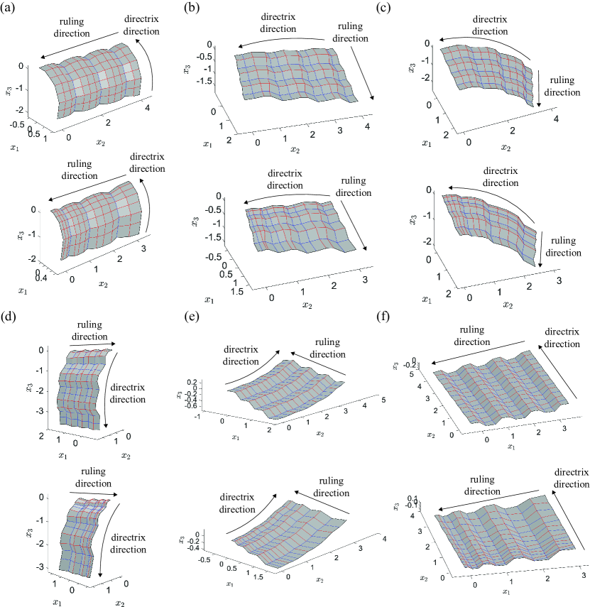
Figure 3: A gallery of quad-mesh rigid origami from repetitive stitching of rectangular units formed from proportional and equimodular couplings. Mountain creases are coloured red and valley creases are coloured blue. For each example, we present a folded state consisting of nine units. More refined meshes can be easily generated in the accompanying MATLAB application (He, 2024) by adjusting the number of units. All these structures display a similar zig-zag pattern, where coordinate polylines along the row or column direction oscillate around a ruling line. Both the ruling and directrix directions are labelled for each example.

Discussion

Our results represent an initial step in advancing the form-finding capabilities of quad-mesh rigid origami beyond the commonly explored (anti-)V-hedra and T-hedra.

Revisiting the levels of surface approximation

One notable difference between the first and second levels of surface approximation is the zig-zag mode in quad-mesh rigid origami. We claim that there is no smooth analogue for developable quad-mesh rigid origami, such as the Miura-ori, anti-V-hedra and developable T-hedra. To elucidate this, it is helpful to introduce the concept of mountain-valley assignment. By assigning an orientation to the discrete surface, we measure the dihedral angle at each crease and subtract it from $\pi$ to determine the folding angle. Creases with negative folding angles are called mountain creases, where the paper bends away from the observer from the specified orientation. Conversely, creases with positive folding angles are called valley creases, where the paper bends towards the observer from the specified orientation. At every developable vertex, the numbers of mountain and valley creases are 3-to-1 or 1-to-3. At every vertex where the sum of sector angles is less than $2\pi$, the mountain and valley creases can be 4-to-0, 3-to-1, 1-to-3 or 0-to-4 in different folded states. At every vertex where the sum of sector angles is more than $2\pi$, the mountain and valley creases can be 3-to-1, 2-to-2, or 1-to-3 in different folded states. This counting of mountain-valley assignments for a degree-4 vertex can be checked both analytically and numerically from He et al. (2023). The coordinate curves and tangent planes around vertices with 3-to-1 or 1-to-3 mountain-valley assignment oscillate when being arbitrarily refined, which is not a feature of a smooth surface. These vertices introduce a zig-zag mode, as illustrated in Figure 1(a), 1(d) and 1(f), though they are not the only cause. In Figure 1(c), alternating rows of 2-to-2 and 0-to-4 vertices can also create this zig-zag mode. Patterns with a smooth analogue, as visualized in Figure 1(b) and 1(e), have a uniform mountain-valley assignment for all interior vertices following 4-to-0, 2-to-2 and 0-to-4 assignments.

In practical origami-based design, we often aim for the metric- and curvature-related properties of the origami structure to closely approximate those of the target surface — beyond merely achieving closeness in distance. The metric-related properties include 1a) arc lengths of coordinate curves; 2a) arc lengths of geodesics; 3a) surface area. Curvature-related properties include 1b) curvature and torsion of coordinate curves; 2b) curvature and torsion of geodesics 3b) normal vector field; 4b) mean curvature; 5b) Gaussian curvature. In classical differential geometry, there are famous examples such as the ‘Staircase paradox’ and the ‘Schwarz lantern’, showcasing the non-convergence of length and area upon the convergence in distance (Section G of the Supplementary Material). From classical mathematical analysis, if a series of discrete curves/surfaces approaches a smooth curve/surface, and all the vertices are exactly on the smooth curve/surface, the tangent plane, metric- and curvature-related properties will converge. We could see that the Staircase and the Schwarz lantern both have a zig-zag mode where the vertices of discrete curves and surfaces are not exactly on the target curve/surface. The examples in Figures 2 and 3 also exhibit this zig-zag pattern, demonstrating non-convergence of the properties listed in 1a) through 3a) and 1b) through 5b). However, this does not imply that all new patterns created through repetitive stitching will exhibit this zig-zag mode.

New semi-discrete quad-mesh rigid origami and curved crease origami with rigid-ruling folding

The new construction method for patterns formed by proportional and equimodular couplings holds strong potential for developing novel semi-discrete quad-mesh rigid origami and curved crease origami with rigid-ruling folding, beyond the current framework based on V-hedra and T-hedra.

A semi-discrete quad-mesh rigid origami involves refining the mesh in only one direction, transforming the creases in this direction into smooth, non-intersecting curves. The resulting pattern is a flexible piecewise smooth surface connected by curved creases. Rigid-ruling folding of curved crease origami is referred to as the continuous isometric deformation of piecewise smooth surfaces jointed by curves (curved creases). This includes semi-discrete quad-mesh rigid origami but also covers scenarios where curved creases intersect. For recent advances we refer the readers to Demaine et al. (2018), Sharifmoghaddam et al. (2023) and Mundilova and Nawratil (2024).

Beyond using repetitive stitching

The periodicity of sector angles in our proposed construction not only reduces the number of constraints, making it fewer than the number of sector angles, but also plays a crucial role in defining the limit smooth surface. However, this represents only the most basic symmetry in generating large quad-mesh rigid origami formed through proportional and equimodular couplings. There remains substantial potential for exploration beyond periodicity.

Self-intersection of the crease pattern

Self-intersection occurs when creases intersect at points other than the specified vertices, a scenario that can emerge during mesh refinement. While preventing self-intersection is essential for practical pattern design, allowing it can provide a method to discretize surface with self-intersecting coordinate curves (Kilian et al., 2024), such as double cone. Resolving this issue requires techniques that lie beyond the scope of this article, and we plan to explore it in future research.

Supplementary Material

This supplementary material serves as an extensive resource for understanding the mathematical principles underlying the new quad-mesh rigid origami emphasized in the main text. In our setup, the sum of sector angles at every interior vertex is not necessarily $2\pi$, which means our discussion includes but is not restricted to developable origami. We include all the necessary derivations towards common quad-mesh origami variants — (anti-)V-hedra and T-hedra, and the more generalized variations reported in the main text — proportional couplings and the equimodular couplings. All the derivations are presented in a detailed manner, ensuring accessibility for researchers across diverse disciplines.

The content is divided into two parts: Part I covers foundational concepts around coordinate nets (i.e. surface patches or parametrization) in both differential geometry and discrete differential geometry. Table LABEL:tab:_notation lists the pertinent notations used throughout this supplementary material. Section A is a supplement to the information of geodesics and Christoffel symbol provided in Do Carmo (2016). Section B introduces common coordinate nets formed by coordinate curves $u_{1}=\mathrm{Const}$ and $u_{2}=\mathrm{Const}$. Section C introduces the well-posed initial condition to obtain these smooth coordinate nets from solving a partial differential equation. Furthermore, in computer graphics and computational mechanics, we are naturally seeking for a ‘nice’ discretization of these coordinate nets. It leads to the introduction on discrete curves and surfaces, together with the matching discrete nets to the aforementioned smooth nets in Section D and Section E. In parallel, Section F introduces the well-posed initial condition to construct these discrete nets as the solution of a partial difference equation. After all these preparation, in Section G we discuss the convergence of a series of discrete nets to a smooth net as the mesh is refined. The above information on discrete nets is mainly from Bobenko and Suris (2008).

Part II is about the information on quad-mesh rigid origami. We concern the continuous isometric (distance-preserving) deformation of both the quad-mesh rigid origami and its Gauss map. The flexibility of quad-mesh rigid origami is introduced in Section H. Common variations, including V-hedra and T-hedra, are detailed in Sections I and J, respectively. For more generalized variations — proportional couplings and equimodular couplings — all relevant details are presented in Sections K, L and M. Finally, evidence supporting our conjecture regarding the limit smooth surface obtained by refining the repetitive stitching of rectangular units is provided in Section N.

Table 1: Notations

Geometrical objects
$X,~{}Y$	a curve or a surface in $\mathbb{R}^{3}$
$x,~{}y$	arbitrary or fixed points in $X$ or $Y$, dependent on context
$x=(x_{1},~{}x_{2},~{}\dots,~{}x_{n})$	coordinates of $x~{}(n\in\mathbb{Z}_{+})$
$I^{n}$	an $n$ dimensional open cube in $\mathbb{R}^{n}~{}(n\in\mathbb{Z}_{+})$. $I$ refers to $(0,~{}1)$ by default.
$O$	an open set
$O(x)$	a neighbourhood at $x$
$\Gamma,~{}\Phi,~{}\Psi$	charts of a curve or a surface. $\Gamma$ is usually used for a curve.
$N$	a unit normal vector
$\mathrm{I},~{}\mathrm{I}_{11},~{}\mathrm{I}_{12},~{}\mathrm{I}_{22}$	the first fundamental form and its components
$\mathrm{II},~{}\mathrm{II}_{11},~{}\mathrm{II}_{12},~{}\mathrm{II}_{22}$	the second fundamental form and its components
$\mathrm{III},~{}\mathrm{III}_{11},~{}\mathrm{III}_{12},~{}\mathrm{III}_{22}$	the third fundamental form and its components
$\kappa,~{}\tau$	curvature and torsion for a curve
$\kappa_{\mathrm{n}},~{}\kappa_{\mathrm{g}}$	the normal curvature and geodesic curvature for a curve on a surface
$\kappa_{1},~{}\kappa_{2},~{}\kappa_{\mathrm{H}},~{}\kappa_{\mathrm{G}}$	the principal curvatures, mean curvature, and Gaussian curvature for a surface.
Parameters
$i,~{}j,~{}k,~{}l$	flexible positive integers or free indices
$m,~{}n$	fixed positive integers
$a,~{}b,~{}c$	scalar or vector parameters in $\mathbb{R}^{n}$ $(n\in\mathbb{Z}_{+})$
$a=(a_{1},~{}a_{2},~{}\dots,~{}a_{n})$	coordinates of $a~{}(n\in\mathbb{Z}_{+})$
$\epsilon,~{}\delta$	real numbers in all forms of $\epsilon-\delta$ expressions
$t,~{}u,~{}v$	parameters for a curve or a surface
$t=(t_{1},~{}t_{2},~{}\dots,~{}t_{m})$	coordinates of $t~{}(m\in\mathbb{Z}_{+})$
$s$	arc length parameter for a curve

Part I Preliminaries in (discrete) differential geometry

Appendix A Geodesic and the Christoffel symbol

Let $X$ be a surface with local chart $\Phi:u=(u_{1},~{}u_{2})\in I^{2}\rightarrow x=(x_{1},~{}x_{2},~{}x_{3})\in X\subset\mathbb{R}^{3}$. In the calculations below, we apply the following regularity condition to all curves and surfaces by default: 1) all local charts are analytic, meaning they are locally represented by convergent power series. As a result, these charts are smooth (have arbitrary order of partial derivatives), with both the charts and their partial derivatives being bounded; 2) the Jacobian $\mathop{}\!\mathrm{d}x/\mathop{}\!\mathrm{d}u$ is of full rank. The normal vector field $N$ on $X$ is:

$$N=\dfrac{\dfrac{\partial x}{\partial u_{1}}\times\dfrac{\partial x}{\partial u_{2}}}{\left|\left|\dfrac{\partial x}{\partial u_{1}}\times\dfrac{\partial x}{\partial u_{2}}\right|\right|}$$

$N:X\rightarrow S^{2}$ is also called the Gauss map, which can be interpreted as translating all the normal vectors of a surface to a unit sphere.

A curve $\Gamma:t\in I\rightarrow x\in X$ on the surface $X$ is a geodesic if there is no ‘lateral acceleration’:

$$\dfrac{\mathop{}\!\mathrm{d}^{2}x}{\mathop{}\!\mathrm{d}t^{2}}\cdot\left(N\times\dfrac{\mathop{}\!\mathrm{d}x}{\mathop{}\!\mathrm{d}t}\right)=0$$

since $\|\mathop{}\!\mathrm{d}x/\mathop{}\!\mathrm{d}s\|=1\Rightarrow(\mathop{}\!\mathrm{d}x/\mathop{}\!\mathrm{d}s)\cdot(\mathop{}\!\mathrm{d}^{2}x/\mathop{}\!\mathrm{d}s^{2})=0$. In the arc length parametrization the above condition is:

$$\begin{gathered}\dfrac{\mathop{}\!\mathrm{d}^{2}x}{\mathop{}\!\mathrm{d}s^{2}}\times N=0~{}~{}\Leftrightarrow~{}~{}\dfrac{\mathop{}\!\mathrm{d}^{2}x}{\mathop{}\!\mathrm{d}s^{2}}=\kappa N,~{}~{}\kappa:I\rightarrow\mathbb{R}\\ \kappa\mathrm{~{}is~{}the~{}curvature~{}of~{}a~{}geodesic~{}}\Gamma\end{gathered}$$

The velocity $\mathop{}\!\mathrm{d}x/\mathop{}\!\mathrm{d}s$ along a geodesic $\Gamma$, as a vector field, is hence said to be parallel on the surface $X$. Clearly, a straight line contained in a surface is a geodesic. Being geodesic is a necessary condition for the shortest path joining two points on a surface.

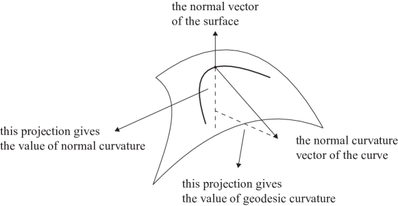
Figure 4: Illustration of the geodesic curvature.

Furthermore, for any curve $\Gamma\subset X$ we have:

$$\dfrac{\mathop{}\!\mathrm{d}^{2}x}{\mathop{}\!\mathrm{d}s^{2}}=\dfrac{1}{\left\|\dfrac{\mathop{}\!\mathrm{d}x}{\mathop{}\!\mathrm{d}t}\right\|}\dfrac{\mathop{}\!\mathrm{d}}{\mathop{}\!\mathrm{d}t}\left(\dfrac{\dfrac{\mathop{}\!\mathrm{d}x}{\mathop{}\!\mathrm{d}t}}{\left\|\dfrac{\mathop{}\!\mathrm{d}x}{\mathop{}\!\mathrm{d}t}\right\|}\right)=\dfrac{1}{\left\|\dfrac{\mathop{}\!\mathrm{d}x}{\mathop{}\!\mathrm{d}t}\right\|^{2}}\left(\dfrac{\mathop{}\!\mathrm{d}^{2}x}{\mathop{}\!\mathrm{d}t^{2}}-\dfrac{\dfrac{\mathop{}\!\mathrm{d}x}{\mathop{}\!\mathrm{d}t}\cdot\dfrac{\mathop{}\!\mathrm{d}^{2}x}{\mathop{}\!\mathrm{d}t^{2}}}{\left\|\dfrac{\mathop{}\!\mathrm{d}x}{\mathop{}\!\mathrm{d}t}\right\|^{2}}\dfrac{\mathop{}\!\mathrm{d}x}{\mathop{}\!\mathrm{d}t}\right)$$

$$\kappa=\left\|\dfrac{\mathop{}\!\mathrm{d}^{2}x}{\mathop{}\!\mathrm{d}s^{2}}\right\|=\dfrac{\left\|\dfrac{\mathop{}\!\mathrm{d}x}{\mathop{}\!\mathrm{d}t}\times\dfrac{\mathop{}\!\mathrm{d}^{2}x}{\mathop{}\!\mathrm{d}t^{2}}\right\|}{\left\|\dfrac{\mathop{}\!\mathrm{d}x}{\mathop{}\!\mathrm{d}t}\right\|^{3}}$$

The (signed) normal curvature $\kappa_{\mathrm{n}}$ is the length of the projection of the acceleration onto the surface normal vector.

$$\kappa_{\mathrm{n}}=\dfrac{\mathop{}\!\mathrm{d}^{2}x}{\mathop{}\!\mathrm{d}s^{2}}\cdot N=\dfrac{\dfrac{\mathop{}\!\mathrm{d}^{2}x}{\mathop{}\!\mathrm{d}t^{2}}\cdot N}{\left\|\dfrac{\mathop{}\!\mathrm{d}x}{\mathop{}\!\mathrm{d}t}\right\|^{2}}$$ (2)

The (signed) geodesic curvature $\kappa_{\mathrm{g}}$ is the length of the projection of the acceleration onto the tangent plane:

$$\kappa_{\mathrm{g}}=\dfrac{\mathop{}\!\mathrm{d}^{2}x}{\mathop{}\!\mathrm{d}s^{2}}\cdot\left(N\times\dfrac{\mathop{}\!\mathrm{d}x}{\mathop{}\!\mathrm{d}s}\right)=\dfrac{\dfrac{\mathop{}\!\mathrm{d}^{2}x}{\mathop{}\!\mathrm{d}t^{2}}\cdot\left(N\times\dfrac{\mathop{}\!\mathrm{d}x}{\mathop{}\!\mathrm{d}t}\right)}{\left\|\dfrac{\mathop{}\!\mathrm{d}x}{\mathop{}\!\mathrm{d}t}\right\|^{3}}$$ (3)

The above definitions lead to

$$\kappa^{2}=\kappa_{\mathrm{n}}^{2}+\kappa_{\mathrm{g}}^{2}$$

Usually we think the curvature or the geodesic curvature is positive if the acceleration $\mathop{}\!\mathrm{d}^{2}x/\mathop{}\!\mathrm{d}s^{2}$ is rotated counterclockwise from the velocity $\mathop{}\!\mathrm{d}x/\mathop{}\!\mathrm{d}s$. This aligns with the right-hand coordinate system such that the normal vector pointing outwards the surface is positive. In other words, the geodesic curvature is the curvature measured from the ‘viewpoint’ on the surface’, which further explains that a geodesic is the analogue of a line on a plane.

$$\Gamma\mathrm{~{}is~{}geodesic~{}}~{}\Leftrightarrow~{}\kappa_{\mathrm{g}}=0\mathrm{~{}~{}along~{}the~{}curve~{}}$$

The Christoffel symbol $\Gamma_{11}^{i},~{}\Gamma_{12}^{i},~{}\Gamma_{22}^{i}~{}(i=1,~{}2)$ denotes how $(\partial^{2}x/\partial u_{1}^{2},~{}\partial^{2}x/\partial u_{1}\partial u_{2},~{}\partial^{2}x/\partial u_{2}^{2})$ is linearly represented by the non-orthogonal frame $(\partial x/\partial u_{1},~{}\partial x/\partial u_{2},~{}N)$:

$$\begin{cases}\dfrac{\partial N}{\partial u_{1}}=a_{11}\dfrac{\partial x}{\partial u_{1}}+a_{21}\dfrac{\partial x}{\partial u_{2}}\\[8.0pt] \dfrac{\partial N}{\partial u_{2}}=a_{12}\dfrac{\partial x}{\partial u_{1}}+a_{22}\dfrac{\partial x}{\partial u_{2}}\\[8.0pt] \dfrac{\partial^{2}x}{\partial u_{1}^{2}}=\Gamma^{1}_{11}\dfrac{\partial x}{\partial u_{1}}+\Gamma^{2}_{11}\dfrac{\partial x}{\partial u_{2}}+b_{11}N\\[8.0pt] \dfrac{\partial^{2}x}{\partial u_{1}\partial u_{2}}=\Gamma^{1}_{12}\dfrac{\partial x}{\partial u_{1}}+\Gamma^{2}_{12}\dfrac{\partial x}{\partial u_{2}}+b_{12}N\\[8.0pt] \dfrac{\partial^{2}x}{\partial u_{2}^{2}}=\Gamma^{1}_{22}\dfrac{\partial x}{\partial u_{1}}+\Gamma^{2}_{22}\dfrac{\partial x}{\partial u_{2}}+b_{22}N\\[8.0pt] \end{cases}$$ (4)

The first two equations in matrix form is:

$$\begin{bmatrix}\dfrac{\partial N}{\partial u_{1}}&\dfrac{\partial N}{\partial u_{2}}\end{bmatrix}=\begin{bmatrix}\dfrac{\partial x}{\partial u_{1}}&\dfrac{\partial x}{\partial u_{2}}\end{bmatrix}\begin{bmatrix}a_{11}&a_{12}\\ a_{21}&a_{22}\end{bmatrix}$$

Note that,

$$||N||\equiv 1~{}~{}\Rightarrow~{}~{}\dfrac{\mathop{}\!\mathrm{d}N}{\mathop{}\!\mathrm{d}u}\cdot N\equiv 0$$

By taking the dot product of $\partial x/\partial u_{1}$ and $\partial x/\partial u_{2}$ with both sides of Eq. (4), we obtain the equations below using the components of the first and second order fundamental form,

$$\begin{dcases}a_{11}\mathrm{I}_{11}+a_{21}\mathrm{I}_{12}=\dfrac{\partial x}{\partial u_{1}}\cdot\dfrac{\partial N}{\partial u_{1}}=\dfrac{\partial}{\partial u_{1}}\left(\dfrac{\partial x}{\partial u_{1}}\cdot N\right)-\mathrm{II}_{11}=-\mathrm{II}_{11}\\ a_{11}\mathrm{I}_{12}+a_{21}\mathrm{I}_{22}=\dfrac{\partial x}{\partial u_{2}}\cdot\dfrac{\partial N}{\partial u_{1}}=\dfrac{\partial}{\partial u_{1}}\left(\dfrac{\partial x}{\partial u_{2}}\cdot N\right)-\mathrm{II}_{12}=-\mathrm{II}_{12}\\ \end{dcases}$$

$$\begin{dcases}a_{12}\mathrm{I}_{11}+a_{22}\mathrm{I}_{12}=\dfrac{\partial x}{\partial u_{1}}\cdot\dfrac{\partial N}{\partial u_{2}}=\dfrac{\partial}{\partial u_{2}}\left(\dfrac{\partial x}{\partial u_{1}}\cdot N\right)-\mathrm{II}_{12}=-\mathrm{II}_{12}\\ a_{12}\mathrm{I}_{12}+a_{22}\mathrm{I}_{22}=\dfrac{\partial x}{\partial u_{2}}\cdot\dfrac{\partial N}{\partial u_{2}}=\dfrac{\partial}{\partial u_{2}}\left(\dfrac{\partial x}{\partial u_{2}}\cdot N\right)-\mathrm{II}_{22}=-\mathrm{II}_{22}\\ \end{dcases}$$

$$\begin{dcases}\Gamma^{1}_{11}\mathrm{I}_{11}+\Gamma^{2}_{11}\mathrm{I}_{12}=\dfrac{\partial x}{\partial u_{1}}\cdot\dfrac{\partial^{2}x}{\partial u_{1}^{2}}=\dfrac{1}{2}\dfrac{\partial\mathrm{I}_{11}}{\partial u_{1}}\\ \Gamma^{1}_{11}\mathrm{I}_{12}+\Gamma^{2}_{11}\mathrm{I}_{22}=\dfrac{\partial x}{\partial u_{2}}\cdot\dfrac{\partial^{2}x}{\partial u_{1}^{2}}=\dfrac{\partial\mathrm{I}_{12}}{\partial u_{1}}-\dfrac{1}{2}\dfrac{\partial\mathrm{I}_{11}}{\partial u_{2}}\\ \end{dcases}$$

$$\begin{dcases}\Gamma^{1}_{12}\mathrm{I}_{11}+\Gamma^{2}_{12}\mathrm{I}_{12}=\dfrac{\partial x}{\partial u_{1}}\cdot\dfrac{\partial^{2}x}{\partial u_{1}\partial u_{2}}=\dfrac{1}{2}\dfrac{\partial\mathrm{I}_{11}}{\partial u_{2}}\\ \Gamma^{1}_{12}\mathrm{I}_{12}+\Gamma^{2}_{12}\mathrm{I}_{22}=\dfrac{\partial x}{\partial u_{2}}\cdot\dfrac{\partial^{2}x}{\partial u_{1}\partial u_{2}}=\dfrac{1}{2}\dfrac{\partial\mathrm{I}_{22}}{\partial u_{1}}\\ \end{dcases}$$

$$\begin{dcases}\Gamma^{1}_{22}\mathrm{I}_{11}+\Gamma^{2}_{22}\mathrm{I}_{12}=\dfrac{\partial x}{\partial u_{1}}\cdot\dfrac{\partial^{2}x}{\partial u_{2}^{2}}=\dfrac{\partial\mathrm{I}_{12}}{\partial u_{2}}-\dfrac{1}{2}\dfrac{\partial\mathrm{I}_{22}}{\partial u_{1}}\\ \Gamma^{1}_{22}\mathrm{I}_{12}+\Gamma^{2}_{22}\mathrm{I}_{22}=\dfrac{\partial x}{\partial u_{2}}\cdot\dfrac{\partial^{2}x}{\partial u_{2}^{2}}=\dfrac{1}{2}\dfrac{\partial\mathrm{I}_{22}}{\partial u_{2}}\\ \end{dcases}$$

Each group of two linear equations have a unique solution since the first fundamental form is positive-definite. More importantly, the Christoffel symbols are fully determined by the first fundamental form hence invariant under isometry.

The components of $a$ are (note that $a_{12}\neq a_{21}$ without extra conditions):

$$\begin{gathered}\begin{bmatrix}\mathrm{I}_{11}&\mathrm{I}_{12}\\ \mathrm{I}_{12}&\mathrm{I}_{22}\end{bmatrix}\begin{bmatrix}a_{11}&a_{12}\\ a_{21}&a_{22}\end{bmatrix}=-\begin{bmatrix}\mathrm{II}_{11}&\mathrm{II}_{12}\\ \mathrm{II}_{12}&\mathrm{II}_{22}\end{bmatrix}\\ \Rightarrow~{}~{}\begin{bmatrix}a_{11}&a_{12}\\ a_{21}&a_{22}\end{bmatrix}=-\begin{bmatrix}\mathrm{I}_{11}&\mathrm{I}_{12}\\ \mathrm{I}_{12}&\mathrm{I}_{22}\end{bmatrix}^{-1}\begin{bmatrix}\mathrm{II}_{11}&\mathrm{II}_{12}\\ \mathrm{II}_{12}&\mathrm{II}_{22}\end{bmatrix}\\ =\dfrac{1}{\mathrm{I}_{11}\mathrm{I}_{22}-\mathrm{I}_{12}^{2}}\begin{bmatrix}-\mathrm{I}_{22}&\mathrm{I}_{12}\\ \mathrm{I}_{12}&-\mathrm{I}_{11}\end{bmatrix}\begin{bmatrix}\mathrm{II}_{11}&\mathrm{II}_{12}\\ \mathrm{II}_{12}&\mathrm{II}_{22}\end{bmatrix}\end{gathered}$$ (5)

and we have

$$\dfrac{\partial N}{\partial u_{1}}\times\dfrac{\partial N}{\partial u_{2}} =(a_{11}a_{22}-a_{12}a_{21})\dfrac{\partial x}{\partial u_{1}}\times\dfrac{\partial x}{\partial u_{2}}$$ (6)

$$=\dfrac{\mathrm{II}_{11}\mathrm{II}_{22}-\mathrm{II}_{12}^{2}}{\mathrm{I}_{11}\mathrm{I}_{22}-\mathrm{I}_{12}^{2}}\dfrac{\partial x}{\partial u_{1}}\times\dfrac{\partial x}{\partial u_{2}}$$

$$=\kappa_{\mathrm{G}}\dfrac{\partial x}{\partial u_{1}}\times\dfrac{\partial x}{\partial u_{2}}$$

The components of $b$ are exactly the components of the second fundamental form. The third fundamental form, which is the first fundamental form of the Gauss map, is defined as:

$$\begin{bmatrix}\mathrm{III}_{11}&\mathrm{III}_{12}\\ \mathrm{III}_{21}&\mathrm{III}_{22}\end{bmatrix}=\begin{bmatrix}\dfrac{\partial N}{\partial u_{1}}\cdot\dfrac{\partial N}{\partial u_{1}}&\dfrac{\partial N}{\partial u_{1}}\cdot\dfrac{\partial N}{\partial u_{2}}\\[12.0pt] \dfrac{\partial N}{\partial u_{2}}\cdot\dfrac{\partial N}{\partial u_{1}}&\dfrac{\partial N}{\partial u_{2}}\cdot\dfrac{\partial N}{\partial u_{2}}\end{bmatrix}$$ (7)

$$\mathrm{III}_{11} =a_{11}^{2}\mathrm{I}_{11}+2a_{11}a_{21}\mathrm{I}_{12}+a_{21}^{2}\mathrm{I}_{22}$$

$$=\begin{bmatrix}a_{11}&a_{21}\end{bmatrix}\begin{bmatrix}\mathrm{I}_{11}&\mathrm{I}_{12}\\ \mathrm{I}_{12}&\mathrm{I}_{22}\end{bmatrix}\begin{bmatrix}a_{11}\\ a_{21}\end{bmatrix}$$

$$\mathrm{III}_{12} =a_{11}a_{12}\mathrm{I}_{11}+(a_{11}a_{22}+a_{21}a_{12})\mathrm{I}_{12}+a_{21}a_{22}\mathrm{I}_{22}$$

$$=\begin{bmatrix}a_{11}&a_{21}\end{bmatrix}\begin{bmatrix}\mathrm{I}_{11}&\mathrm{I}_{12}\\ \mathrm{I}_{12}&\mathrm{I}_{22}\end{bmatrix}\begin{bmatrix}a_{12}\\ a_{22}\end{bmatrix}$$

$$\mathrm{III}_{22} =a_{12}^{2}\mathrm{I}_{11}+2a_{12}a_{22}\mathrm{I}_{12}+a_{12}^{2}\mathrm{I}_{22}$$

$$=\begin{bmatrix}a_{12}&a_{22}\end{bmatrix}\begin{bmatrix}\mathrm{I}_{11}&\mathrm{I}_{12}\\ \mathrm{I}_{12}&\mathrm{I}_{22}\end{bmatrix}\begin{bmatrix}a_{12}\\ a_{22}\end{bmatrix}$$

We could see that

$$\begin{bmatrix}\mathrm{III}_{11}&\mathrm{III}_{12}\\ \mathrm{III}_{12}&\mathrm{III}_{22}\end{bmatrix} =\begin{bmatrix}a_{11}&a_{12}\\ a_{21}&a_{22}\end{bmatrix}^{\mathrm{T}}\begin{bmatrix}\mathrm{I}_{11}&\mathrm{I}_{12}\\ \mathrm{I}_{12}&\mathrm{I}_{22}\end{bmatrix}\begin{bmatrix}a_{11}&a_{12}\\ a_{21}&a_{22}\end{bmatrix}$$

$$=\dfrac{1}{\mathrm{I}_{11}\mathrm{I}_{22}-\mathrm{I}_{12}^{2}}\begin{bmatrix}\mathrm{II}_{11}&\mathrm{II}_{12}\\ \mathrm{II}_{12}&\mathrm{II}_{22}\end{bmatrix}\begin{bmatrix}\mathrm{I}_{22}&-\mathrm{I}_{12}\\ -\mathrm{I}_{12}&\mathrm{I}_{11}\end{bmatrix}\begin{bmatrix}\mathrm{II}_{11}&\mathrm{II}_{12}\\ \mathrm{II}_{12}&\mathrm{II}_{22}\end{bmatrix}$$

$$\begin{gathered}\mathrm{III}_{11}=\dfrac{\mathrm{II}_{12}^{2}\mathrm{I}_{11}-2\mathrm{II}_{11}\mathrm{II}_{22}\mathrm{I}_{12}+\mathrm{II}_{11}^{2}\mathrm{I}_{22}}{\mathrm{I}_{11}\mathrm{I}_{22}-\mathrm{I}_{12}^{2}}\\ \mathrm{III}_{12}=\dfrac{\mathrm{II}_{12}\mathrm{II}_{22}\mathrm{I}_{11}-(\mathrm{II}_{11}\mathrm{II}_{22}+\mathrm{II}_{12}^{2})\mathrm{I}_{12}+\mathrm{II}_{11}\mathrm{II}_{12}\mathrm{I}_{22}}{\mathrm{I}_{11}\mathrm{I}_{22}-\mathrm{I}_{12}^{2}}\\ \mathrm{III}_{22}=\dfrac{\mathrm{II}_{22}^{2}\mathrm{I}_{11}-2\mathrm{II}_{12}\mathrm{II}_{22}\mathrm{I}_{12}+\mathrm{II}_{12}^{2}\mathrm{I}_{22}}{\mathrm{I}_{11}\mathrm{I}_{22}-\mathrm{I}_{12}^{2}}\end{gathered}$$

$$\begin{bmatrix}\mathrm{III}_{11}&\mathrm{III}_{12}\\ \mathrm{III}_{12}&\mathrm{III}_{22}\end{bmatrix}=-\dfrac{\mathrm{II}_{11}\mathrm{II}_{22}-\mathrm{II}_{12}^{2}}{\mathrm{I}_{11}\mathrm{I}_{22}-\mathrm{I}_{12}^{2}}\begin{bmatrix}\mathrm{I}_{11}&\mathrm{I}_{12}\\ \mathrm{I}_{12}&\mathrm{I}_{22}\end{bmatrix}+\dfrac{\mathrm{II}_{22}\mathrm{I}_{11}-2\mathrm{II}_{12}\mathrm{I}_{12}+\mathrm{II}_{11}\mathrm{I}_{22}}{\mathrm{I}_{11}\mathrm{I}_{22}-\mathrm{I}_{12}^{2}}\begin{bmatrix}\mathrm{II}_{11}&\mathrm{II}_{12}\\ \mathrm{II}_{12}&\mathrm{II}_{22}\end{bmatrix}$$

In conclusion:

$$\begin{bmatrix}\mathrm{III}_{11}&\mathrm{III}_{12}\\ \mathrm{III}_{12}&\mathrm{III}_{22}\end{bmatrix}=-\kappa_{\mathrm{G}}\begin{bmatrix}\mathrm{I}_{11}&\mathrm{I}_{12}\\ \mathrm{I}_{12}&\mathrm{I}_{22}\end{bmatrix}+2\kappa_{\mathrm{H}}\begin{bmatrix}\mathrm{II}_{11}&\mathrm{II}_{12}\\ \mathrm{II}_{12}&\mathrm{II}_{22}\end{bmatrix}$$ (8)

The explicit expression of the Christoffel symbol is:

$$\begin{gathered}\Gamma_{11}^{1}=\dfrac{\dfrac{\mathrm{I}_{22}}{2}\dfrac{\partial\mathrm{I}_{11}}{\partial u_{1}}-\mathrm{I}_{12}\left(\dfrac{\partial\mathrm{I}_{12}}{\partial u_{1}}-\dfrac{1}{2}\dfrac{\partial\mathrm{I}_{11}}{\partial u_{2}}\right)}{\mathrm{I}_{11}\mathrm{I}_{22}-\mathrm{I}_{12}^{2}}\\ \Gamma_{11}^{2}=\dfrac{\mathrm{I}_{11}\left(\dfrac{\partial\mathrm{I}_{12}}{\partial u_{1}}-\dfrac{1}{2}\dfrac{\partial\mathrm{I}_{11}}{\partial u_{2}}\right)-\dfrac{\mathrm{I}_{12}}{2}\dfrac{\partial\mathrm{I}_{11}}{\partial u_{1}}}{\mathrm{I}_{11}\mathrm{I}_{22}-\mathrm{I}_{12}^{2}}\end{gathered}$$

$$\begin{gathered}\Gamma_{12}^{1}=\dfrac{\dfrac{\mathrm{I}_{22}}{2}\dfrac{\partial\mathrm{I}_{11}}{\partial u_{2}}-\dfrac{\mathrm{I}_{12}}{2}\dfrac{\partial\mathrm{I}_{22}}{\partial u_{1}}}{\mathrm{I}_{11}\mathrm{I}_{22}-\mathrm{I}_{12}^{2}}\\ \Gamma_{12}^{2}=\dfrac{\dfrac{\mathrm{I}_{11}}{2}\dfrac{\partial\mathrm{I}_{22}}{\partial u_{1}}-\dfrac{\mathrm{I}_{12}}{2}\dfrac{\partial\mathrm{I}_{11}}{\partial u_{2}}}{\mathrm{I}_{11}\mathrm{I}_{22}-\mathrm{I}_{12}^{2}}\end{gathered}$$ (9)

$$\begin{gathered}\Gamma_{22}^{1}=\dfrac{\mathrm{I}_{22}\left(\dfrac{\partial\mathrm{I}_{12}}{\partial u_{2}}-\dfrac{1}{2}\dfrac{\partial\mathrm{I}_{22}}{\partial u_{1}}\right)-\dfrac{\mathrm{I}_{12}}{2}\dfrac{\partial\mathrm{I}_{22}}{\partial u_{2}}}{\mathrm{I}_{11}\mathrm{I}_{22}-\mathrm{I}_{12}^{2}}\\ \Gamma_{22}^{2}=\dfrac{\dfrac{\mathrm{I}_{11}}{2}\dfrac{\partial\mathrm{I}_{22}}{\partial u_{2}}-\mathrm{I}_{12}\left(\dfrac{\partial\mathrm{I}_{12}}{\partial u_{2}}-\dfrac{1}{2}\dfrac{\partial\mathrm{I}_{22}}{\partial u_{1}}\right)}{\mathrm{I}_{11}\mathrm{I}_{22}-\mathrm{I}_{12}^{2}}\end{gathered}$$

Notably the following compatibility condition relates the first and second fundamental forms.

$$\begin{cases}\dfrac{\partial}{\partial u_{2}}\left(\dfrac{\partial^{2}x}{\partial u_{1}^{2}}\right)=\dfrac{\partial}{\partial u_{1}}\left(\dfrac{\partial^{2}x}{\partial u_{1}\partial u_{2}}\right)\\[8.0pt] \dfrac{\partial}{\partial u_{1}}\left(\dfrac{\partial^{2}x}{\partial u_{2}^{2}}\right)=\dfrac{\partial}{\partial u_{2}}\left(\dfrac{\partial^{2}x}{\partial u_{1}\partial u_{2}}\right)\\[8.0pt] \dfrac{\partial}{\partial u_{2}}\left(\dfrac{\partial N}{\partial u_{1}}\right)=\dfrac{\partial}{\partial u_{1}}\left(\dfrac{\partial N}{\partial u_{2}}\right)\\ \end{cases}$$

by writing everything under the basis $(\partial x/\partial u_{1},~{}\partial x/\partial u_{2},~{}N)$ and comparing the coefficient, we could obtain 9 relations among the first and second fundamental forms. It turns out that only 3 of them are independent, called the compatibility equation of surfaces or Gauss-Mainardi-Codazzi Equations:

$$\begin{dcases}\dfrac{\partial\Gamma^{2}_{12}}{\partial u_{1}}-\dfrac{\partial\Gamma^{2}_{11}}{\partial u_{2}}+\Gamma^{1}_{12}\Gamma^{2}_{11}+\Gamma^{2}_{12}\Gamma^{2}_{12}-\Gamma^{2}_{11}\Gamma^{2}_{22}-\Gamma^{1}_{11}\Gamma^{2}_{12}=-\mathrm{I}_{11}\kappa_{\mathrm{G}}\\ \dfrac{\partial\mathrm{II}_{11}}{\partial u_{2}}-\dfrac{\partial\mathrm{II}_{12}}{\partial u_{1}}=\mathrm{II}_{11}\Gamma^{1}_{12}+\mathrm{II}_{12}(\Gamma^{2}_{12}-\Gamma^{1}_{11})-\mathrm{II}_{22}\Gamma^{2}_{11}\\ \dfrac{\partial\mathrm{II}_{12}}{\partial u_{2}}-\dfrac{\partial\mathrm{II}_{22}}{\partial u_{1}}=\mathrm{II}_{11}\Gamma^{1}_{22}+\mathrm{II}_{12}(\Gamma^{2}_{22}-\Gamma^{1}_{12})-\mathrm{II}_{22}\Gamma^{2}_{12}\\ \end{dcases}$$ (10)

Appendix B Coordinate net

Let $X$ be a parametrized surface with chart $\Phi:u\in I^{2}\rightarrow x\in X\subset\mathbb{R}^{3}$. The coordinate curves described by $u_{1}=\mathrm{Const}$ and $u_{2}=\mathrm{Const}$, forms a coordinate net on $X$. The angle $\theta$ between coordinate curves, which can be calculated using

$$\cos\theta=\dfrac{\mathrm{I}_{12}}{\sqrt{\mathrm{I}_{11}\mathrm{I}_{22}}}$$

is called the Chebyshev angle. The study on coordinate nets are extremely useful for our interests since it provides a natural discretization to a quad-mesh.

Recall that we simplify the parametrization of a curve by using arc length. If we take a similar operation:

$$\begin{gathered}s_{1}=\int_{0}^{u_{1}}\sqrt{\mathrm{I}_{11}(v_{1},~{}v_{2})}\mathop{}\!\mathrm{d}v_{1}\\ s_{2}=\int_{0}^{u_{2}}\sqrt{\mathrm{I}_{22}(v_{1},~{}v_{2})}\mathop{}\!\mathrm{d}v_{2}\end{gathered}$$

since

$$\begin{gathered}\dfrac{\partial x}{\partial s_{1}}=\dfrac{\partial x}{\partial u_{1}}\dfrac{\partial u_{1}}{\partial s_{1}}+\dfrac{\partial x}{\partial u_{2}}\dfrac{\partial u_{2}}{\partial s_{1}}\\ \dfrac{\partial x}{\partial s_{2}}=\dfrac{\partial x}{\partial u_{1}}\dfrac{\partial u_{1}}{\partial s_{2}}+\dfrac{\partial x}{\partial u_{2}}\dfrac{\partial u_{2}}{\partial s_{2}}\\ \end{gathered}$$

the arc length reparametrization does not make any simplification. However, observe that if

$$\dfrac{\partial\mathrm{I}_{11}}{\partial u_{2}}=\dfrac{\partial\mathrm{I}_{22}}{\partial u_{1}}=0$$

which means the lengths of the opposite side of ‘curved quadrilaterals’ formed by the coordinate curves are equal. We can use the above arc length parametrization $s=(s_{1},~{}s_{2})$, called a Chebyshev net, such that

$$\begin{bmatrix}\mathrm{I}_{11}&\mathrm{I}_{12}\\ \mathrm{I}_{12}&\mathrm{I}_{22}\end{bmatrix}=\begin{bmatrix}1&\cos\theta\\ \cos\theta&1\end{bmatrix},~{}~{}\theta\in(0,\pi)\textrm{~{}is~{}the~{}Chebyshev~{}angle~{}}$$

Note that the condition for a Chebyshev net is equivalent to

$$\begin{dcases}\dfrac{1}{2}\dfrac{\partial\mathrm{I}_{11}}{\partial u_{2}}=\dfrac{\partial^{2}x}{\partial u_{1}\partial u_{2}}\cdot\dfrac{\partial x}{\partial u_{1}}=0\\ \dfrac{1}{2}\dfrac{\partial\mathrm{I}_{22}}{\partial u_{1}}=\dfrac{\partial^{2}x}{\partial u_{1}\partial u_{2}}\cdot\dfrac{\partial x}{\partial u_{2}}=0\\ \end{dcases}~{}~{}\Leftrightarrow~{}~{}\begin{dcases}\dfrac{\partial^{2}x}{\partial u_{1}\partial u_{2}}=\lambda(u_{1},~{}u_{2})\dfrac{\partial x}{\partial u_{1}}\times\dfrac{\partial x}{\partial u_{2}}\\ \lambda:I^{2}\rightarrow\mathbb{R}\end{dcases}$$ (11)

which is the differential equation for a Chebyshev net. The ratio $\lambda(u),~{}u=(u_{1},~{}u_{2})\in I^{2}$ is:

$$\lambda(u)=\dfrac{\dfrac{\partial^{2}x}{\partial u_{1}\partial u_{2}}\cdot N}{\left\|\dfrac{\partial x}{\partial u_{1}}\times\dfrac{\partial x}{\partial u_{2}}\right\|}=\dfrac{\mathrm{I}_{12}}{\sqrt{\mathrm{I}_{11}\mathrm{I}_{22}-\mathrm{I}_{12}^{2}}}$$ (12)

The Christoffel symbols and Gaussian curvature from direct calculation over the first fundamental form is:

$$\begin{gathered}\Gamma_{11}^{1}=\dfrac{1}{\tan\theta}\dfrac{\partial\theta}{\partial s_{1}},~{}~{}\Gamma_{11}^{2}=-\dfrac{1}{\sin\theta}\dfrac{\partial\theta}{\partial s_{1}}\\ \Gamma_{12}^{1}=\Gamma_{12}^{2}=0\\ \Gamma_{22}^{1}=-\dfrac{1}{\sin\theta}\dfrac{\partial\theta}{\partial s_{2}},~{}~{}\Gamma_{22}^{2}=\dfrac{1}{\tan\theta}\dfrac{\partial\theta}{\partial s_{2}}\end{gathered}$$

$$\kappa_{\mathrm{G}}=-\dfrac{1}{\sin\theta}\dfrac{\partial^{2}\theta}{\partial s_{1}\partial s_{2}}$$

In particular, an orthogonal Chebyshev net where $\mathrm{I}_{12}=0$ everywhere infers that $\theta=\pi/2$ identically. The Gaussian curvature $\kappa_{\mathrm{G}}=0$ from the above calculation.

Recall that an asymptotic curve on a surface has everywhere zero normal curvature. We say a parametrization forms an asymptotic net if both coordinate curves are asymptotic curves, which means:

$$\begin{dcases}\begin{bmatrix}1&0\end{bmatrix}\begin{bmatrix}\mathrm{II}_{11}&\mathrm{II}_{12}\\ \mathrm{II}_{12}&\mathrm{II}_{22}\end{bmatrix}\begin{bmatrix}1\\ 0\end{bmatrix}=0\\ \begin{bmatrix}0&1\end{bmatrix}\begin{bmatrix}\mathrm{II}_{11}&\mathrm{II}_{12}\\ \mathrm{II}_{12}&\mathrm{II}_{22}\end{bmatrix}\begin{bmatrix}0\\ 1\end{bmatrix}=0\end{dcases}~{}~{}\Leftrightarrow~{}~{}\mathrm{II}_{11}=0,~{}\mathrm{II}_{22}=0$$ (13)

The derivative of the Gauss map of an asymptotic net can be derived from Eq. (5):

$$\begin{bmatrix}\dfrac{\partial N}{\partial u_{1}}&\dfrac{\partial N}{\partial u_{2}}\end{bmatrix} =\dfrac{1}{\mathrm{I}_{11}\mathrm{I}_{22}-\mathrm{I}_{12}^{2}}\begin{bmatrix}\dfrac{\partial x}{\partial u_{1}}&\dfrac{\partial x}{\partial u_{2}}\end{bmatrix}\begin{bmatrix}-\mathrm{I}_{22}&\mathrm{I}_{12}\\ \mathrm{I}_{12}&-\mathrm{I}_{11}\end{bmatrix}\begin{bmatrix}\mathrm{II}_{11}&\mathrm{II}_{12}\\ \mathrm{II}_{12}&\mathrm{II}_{22}\end{bmatrix}$$ (14)

$$=\dfrac{\mathrm{II}_{12}}{\mathrm{I}_{11}\mathrm{I}_{22}-\mathrm{I}_{12}^{2}}\begin{bmatrix}\dfrac{\partial x}{\partial u_{1}}&\dfrac{\partial x}{\partial u_{2}}\end{bmatrix}\begin{bmatrix}\mathrm{I}_{12}&-\mathrm{I}_{22}\\ -\mathrm{I}_{11}&\mathrm{I}_{12}\end{bmatrix}$$

Since

$$N=\dfrac{\dfrac{\partial x}{\partial u_{1}}\times\dfrac{\partial x}{\partial u_{2}}}{\left\|\dfrac{\partial x}{\partial u_{1}}\times\dfrac{\partial x}{\partial u_{2}}\right\|}=\dfrac{\dfrac{\partial x}{\partial u_{1}}\times\dfrac{\partial x}{\partial u_{2}}}{\sqrt{\mathrm{I}_{11}\mathrm{I}_{22}-\mathrm{I}_{12}^{2}}}$$

$$\begin{gathered}N\times\dfrac{\partial x}{\partial u_{1}}=\dfrac{1}{\sqrt{\mathrm{I}_{11}\mathrm{I}_{22}-\mathrm{I}_{12}^{2}}}\left(\mathrm{I}_{11}\dfrac{\partial x}{\partial u_{2}}-\mathrm{I}_{12}\dfrac{\partial x}{\partial u_{1}}\right)\\ \dfrac{\partial x}{\partial u_{2}}\times N=\dfrac{1}{\sqrt{\mathrm{I}_{11}\mathrm{I}_{22}-\mathrm{I}_{12}^{2}}}\left(\mathrm{I}_{22}\dfrac{\partial x}{\partial u_{1}}-\mathrm{I}_{12}\dfrac{\partial x}{\partial u_{2}}\right)\end{gathered}$$ (15)

we have (note that $\kappa_{\mathrm{G}}<0$ since $\mathrm{II}_{11}=\mathrm{II}_{22}=0$)

$$\begin{gathered}N\times\dfrac{\partial N}{\partial u_{1}}=\dfrac{\mathrm{II}_{12}}{\sqrt{\mathrm{I}_{11}\mathrm{I}_{22}-\mathrm{I}_{12}^{2}}}\dfrac{\partial x}{\partial u_{1}}=(-\kappa_{\mathrm{G}})^{1/2}\dfrac{\partial x}{\partial u_{1}}\\ \dfrac{\partial N}{\partial u_{2}}\times N=\dfrac{\mathrm{II}_{12}}{\sqrt{\mathrm{I}_{11}\mathrm{I}_{22}-\mathrm{I}_{12}^{2}}}\dfrac{\partial x}{\partial u_{2}}=(-\kappa_{\mathrm{G}})^{1/2}\dfrac{\partial x}{\partial u_{2}}\end{gathered}$$ (16)

The Lelieuvre normal field $N^{\mathrm{L}}$ is defined as (Blaschke, 1923):

$$N^{\mathrm{L}}=N(-\kappa_{\mathrm{G}})^{-1/4}$$ (17)

which satisfies:

$$\begin{gathered}N^{\mathrm{L}}\times\dfrac{\partial N^{\mathrm{L}}}{\partial u_{1}}=\dfrac{\partial x}{\partial u_{1}}\\ \dfrac{\partial N^{\mathrm{L}}}{\partial u_{2}}\times N^{\mathrm{L}}=\dfrac{\partial x}{\partial u_{2}}\end{gathered}$$ (18)

Furthermore,

$$\begin{gathered}\dfrac{1}{2}\left(\dfrac{\partial}{\partial u_{1}}\left(\dfrac{\partial N^{\mathrm{L}}}{\partial u_{2}}\times N^{\mathrm{L}}\right)-\dfrac{\partial}{\partial u_{2}}\left(N^{\mathrm{L}}\times\dfrac{\partial N^{\mathrm{L}}}{\partial u_{1}}\right)\right)=\dfrac{\partial^{2}N^{\mathrm{L}}}{\partial u_{1}\partial u_{2}}\times N^{\mathrm{L}}=0\\ \dfrac{1}{2}\left(\dfrac{\partial}{\partial u_{1}}\left(\dfrac{\partial N^{\mathrm{L}}}{\partial u_{2}}\times N^{\mathrm{L}}\right)+\dfrac{\partial}{\partial u_{2}}\left(N^{\mathrm{L}}\times\dfrac{\partial N^{\mathrm{L}}}{\partial u_{1}}\right)\right)=\dfrac{\partial N^{\mathrm{L}}}{\partial u_{2}}\times\dfrac{\partial N^{\mathrm{L}}}{\partial u_{1}}=\dfrac{\partial^{2}x}{\partial u_{1}\partial u_{2}}\\ \end{gathered}$$ (19)

We say $N^{\mathrm{L}}$ is Lorentz-harmonic and forms a Moutard net if:

$$\dfrac{\partial^{2}N^{\mathrm{L}}}{\partial u_{1}\partial u_{2}}=\lambda N^{\mathrm{L}},~{}~{}\lambda:I^{2}\rightarrow\mathbb{R}$$ (20)

Given a Moutard net $N^{\mathrm{L}}$, from Eq. (18) and the integration of $\partial x/\partial s_{1}$ and $\partial x/\partial s_{2}$ we could obtain a unique surface $x$, up to a translation.

Now we consider an asymptotic Chebyshev net, as known as a K-surface in previous literatures. From the compatibility equation of surfaces, Eq. (10), an asymptotic Chebyshev net has the second fundamental form below:

$$\begin{bmatrix}\mathrm{II}_{11}&\mathrm{II}_{12}\\ \mathrm{II}_{12}&\mathrm{II}_{22}\end{bmatrix}=\begin{bmatrix}0&\sin\theta\\ \sin\theta&0\end{bmatrix}$$

and we could obtain

$$\begin{gathered}\kappa_{\mathrm{G}}=-1\\ \dfrac{\partial^{2}\theta}{\partial s_{1}\partial s_{2}}=\sin\theta\end{gathered}$$ (21)

To conclude, only a pseudosphere admits an asymptotic Chebyshev net. The latter is the famous sine-Gordon equation. Immediately from Eq. (16):

$$\begin{dcases}\dfrac{\partial x}{\partial s_{1}}=N\times\dfrac{\partial N}{\partial s_{1}}\\ \dfrac{\partial x}{\partial s_{2}}=\dfrac{\partial N}{\partial s_{2}}\times N\\ \end{dcases}$$ (22)

then from Eq. (19) and Eq. (6):

$$\dfrac{\partial^{2}x}{\partial s_{1}\partial s_{2}}=-\dfrac{\partial N}{\partial s_{1}}\times\dfrac{\partial N}{\partial s_{2}}=-\kappa_{\mathrm{G}}\dfrac{\partial x}{\partial s_{1}}\times\dfrac{\partial x}{\partial s_{2}}=-\kappa_{\mathrm{G}}\sqrt{\mathrm{I}_{11}\mathrm{I}_{22}-\mathrm{I}_{12}^{2}}N=N\sin\theta$$ (23)

which means

$$\dfrac{\partial^{2}x}{\partial s_{1}\partial s_{2}}\times N=0~{}~{}\Leftrightarrow~{}~{}\begin{dcases}\dfrac{\partial^{2}x}{\partial s_{1}\partial s_{2}}\cdot\dfrac{\partial x}{\partial s_{1}}=\dfrac{1}{2}\dfrac{\partial\mathrm{I}_{11}}{\partial s_{2}}=0\\ \dfrac{\partial^{2}x}{\partial s_{1}\partial s_{2}}\cdot\dfrac{\partial x}{\partial s_{2}}=\dfrac{1}{2}\dfrac{\partial\mathrm{I}_{22}}{\partial s_{1}}=0\end{dcases}$$

Now continue from Eq. (5):

$$\begin{bmatrix}\dfrac{\partial N}{\partial s_{1}}&\dfrac{\partial N}{\partial s_{2}}\end{bmatrix} =\dfrac{\mathrm{II}_{12}}{\mathrm{I}_{11}\mathrm{I}_{22}-\mathrm{I}_{12}^{2}}\begin{bmatrix}\dfrac{\partial x}{\partial s_{1}}&\dfrac{\partial x}{\partial s_{2}}\end{bmatrix}\begin{bmatrix}\mathrm{I}_{12}&-\mathrm{I}_{22}\\ -\mathrm{I}_{11}&\mathrm{I}_{12}\end{bmatrix}$$ (24)

$$=\begin{bmatrix}\dfrac{\partial x}{\partial s_{1}}&\dfrac{\partial x}{\partial s_{2}}\end{bmatrix}\begin{bmatrix}\dfrac{1}{\tan\theta}&-\dfrac{1}{\sin\theta}\\[10.0pt] -\dfrac{1}{\sin\theta}&\dfrac{1}{\tan\theta}\end{bmatrix}$$

From direct calculation we could see that:

$$\dfrac{\partial^{2}N}{\partial s_{1}\partial s_{2}}= -\left(1+\dfrac{1}{\tan^{2}\theta}\right)\dfrac{\partial\theta}{\partial s_{2}}\dfrac{\partial x}{\partial s_{1}}+\dfrac{1}{\tan\theta}\dfrac{\partial^{2}x}{\partial s_{1}\partial s_{2}}+\dfrac{1}{\sin\theta\tan\theta}\dfrac{\partial\theta}{\partial s_{2}}\dfrac{\partial x}{\partial s_{2}}-\dfrac{1}{\sin\theta}\dfrac{\partial^{2}x}{\partial s_{2}^{2}}$$

$$= -\left(1+\dfrac{1}{\tan^{2}\theta}\right)\dfrac{\partial\theta}{\partial s_{1}}\dfrac{\partial x}{\partial s_{2}}+\dfrac{1}{\tan\theta}\dfrac{\partial^{2}x}{\partial s_{1}\partial s_{2}}+\dfrac{1}{\sin\theta\tan\theta}\dfrac{\partial\theta}{\partial s_{1}}\dfrac{\partial x}{\partial s_{1}}-\dfrac{1}{\sin\theta}\dfrac{\partial^{2}x}{\partial s_{1}^{2}}$$

Since

$$\dfrac{\partial^{2}x}{\partial s_{1}\partial s_{2}}\cdot\dfrac{\partial x}{\partial s_{1}}=\dfrac{\partial\mathrm{I}_{11}}{\partial s_{2}}=0,~{}~{}\dfrac{\partial^{2}x}{\partial s_{1}\partial s_{2}}\cdot\dfrac{\partial x}{\partial s_{2}}=\dfrac{\partial\mathrm{I}_{22}}{\partial s_{1}}=0$$

$$\dfrac{\partial^{2}x}{\partial s_{1}^{2}}\cdot\dfrac{\partial x}{\partial s_{1}}=\dfrac{\partial\mathrm{I}_{11}}{\partial s_{1}}=0,~{}~{}\dfrac{\partial^{2}x}{\partial s_{2}^{2}}\cdot\dfrac{\partial x}{\partial s_{2}}=\dfrac{\partial\mathrm{I}_{22}}{\partial s_{2}}=0$$

$$\dfrac{\partial^{2}x}{\partial s_{1}^{2}}\cdot\dfrac{\partial x}{\partial s_{2}}=\dfrac{\partial\mathrm{I}_{12}}{\partial s_{1}}-\dfrac{\partial^{2}x}{\partial s_{1}\partial s_{2}}\cdot\dfrac{\partial x}{\partial s_{1}}=-\sin\theta\dfrac{\partial\theta}{\partial s_{1}}$$

$$\dfrac{\partial^{2}x}{\partial s_{2}^{2}}\cdot\dfrac{\partial x}{\partial s_{1}}=\dfrac{\partial\mathrm{I}_{12}}{\partial s_{2}}-\dfrac{\partial^{2}x}{\partial s_{1}\partial s_{2}}\cdot\dfrac{\partial x}{\partial s_{2}}=-\sin\theta\dfrac{\partial\theta}{\partial s_{2}}$$

For both expressions of $\partial^{2}N/\partial s_{1}\partial s_{2}$, from dot production over $\partial^{2}x/\partial s_{1}$ and $\partial^{2}x/\partial s_{2}$:

$$\dfrac{\partial^{2}N}{\partial s_{1}\partial s_{2}}\cdot\dfrac{\partial x}{\partial s_{1}}=0$$

$$\dfrac{\partial^{2}N}{\partial s_{1}\partial s_{2}}\cdot\dfrac{\partial x}{\partial s_{2}}=0$$

We conclude that the Moutard equation for $N$ is:

$$\dfrac{\partial^{2}N}{\partial s_{1}\partial s_{2}}=N\cos\theta$$ (25)

Furthermore we could see that:

$$\begin{gathered}\dfrac{\partial^{2}N}{\partial s_{1}\partial s_{2}}\cdot\dfrac{\partial N}{\partial s_{1}}=0~{}~{}\Rightarrow~{}~{}\dfrac{\partial}{\partial s_{2}}\left(\dfrac{\partial N}{\partial s_{1}}\cdot\dfrac{\partial N}{\partial s_{1}}\right)=0\\ \dfrac{\partial^{2}N}{\partial s_{1}\partial s_{2}}\cdot\dfrac{\partial N}{\partial s_{2}}=0~{}~{}\Rightarrow~{}~{}\dfrac{\partial}{\partial s_{1}}\left(\dfrac{\partial N}{\partial s_{2}}\cdot\dfrac{\partial N}{\partial s_{2}}\right)=0\end{gathered}$$

The above derivation leads to the following proposition:

Proposition 1.

The Gauss map of a K-surface is a Chebyshev net. A K-surface is the only asymptotic net with a Chebyshev Gauss map.

The counterpart of an asymptotic net is a geodesic net, where the coordinate curves have everywhere zero geodesic curvature. Note that even though the velocity along coordinate curves are constant, it will change along the other direction hence there is no arc length reparametrization similar to the Chebyshev net. The condition for a parametrization $u$ to form a geodesic net is the geodesic curvature is everywhere zero for each coordinate curve. From Eq. (3)

$$\begin{dcases}\dfrac{\partial^{2}x}{\partial u_{1}^{2}}\cdot\left(N\times\dfrac{\partial x}{\partial u_{1}}\right)=0\\ \dfrac{\partial^{2}x}{\partial u_{2}^{2}}\cdot\left(N\times\dfrac{\partial x}{\partial u_{2}}\right)=0\\ \end{dcases}$$

It says $\mathop{}\!\mathrm{d}^{2}x/\mathop{}\!\mathrm{d}u_{1}^{2}$ can be linearly represented by $N$ and $\mathop{}\!\mathrm{d}x/\mathop{}\!\mathrm{d}u_{1}$; $\mathop{}\!\mathrm{d}^{2}x/\mathop{}\!\mathrm{d}u_{2}^{2}$ can be linearly represented by $N$ and $\mathop{}\!\mathrm{d}x/\mathop{}\!\mathrm{d}u_{2}$. From Eq. (4), this condition is equivalent to certain Christoffel symbols are zero:

$$\Gamma_{11}^{2}=\Gamma_{22}^{1}=0$$

and we can write the condition above in terms of the components of the first fundamental form from Eq. (9):

$$\begin{dcases}2\mathrm{I}_{11}\dfrac{\partial\mathrm{I}_{12}}{\partial u_{1}}=\mathrm{I}_{11}\dfrac{\partial\mathrm{I}_{11}}{\partial u_{2}}+\mathrm{I}_{12}\dfrac{\partial\mathrm{I}_{11}}{\partial u_{1}}\\ 2\mathrm{I}_{22}\dfrac{\partial\mathrm{I}_{12}}{\partial u_{2}}=\mathrm{I}_{22}\dfrac{\partial\mathrm{I}_{22}}{\partial u_{1}}+\mathrm{I}_{12}\dfrac{\partial\mathrm{I}_{22}}{\partial u_{2}}\\ \end{dcases}$$ (26)

Eq. (26) is the condition for a chart to form a geodesic net. Furthermore, let $\mathrm{I}_{12}=0$, we obtain $\partial\mathrm{I}_{11}/\partial u_{2}=\partial\mathrm{I}_{22}/\partial u_{1}=0$. Therefore an orthogonal geodesic net is equivalent to an orthogonal Chebyshev net. The first fundamental form is an identity matrix and $\kappa_{\mathrm{G}}=0$.

Two tangent vectors

$$\begin{gathered}\dfrac{\mathop{}\!\mathrm{d}x}{\mathop{}\!\mathrm{d}u}\begin{bmatrix}a_{1}\\ a_{2}\end{bmatrix},~{}~{}\dfrac{\mathop{}\!\mathrm{d}x}{\mathop{}\!\mathrm{d}u}\begin{bmatrix}b_{1}\\ b_{2}\end{bmatrix},~{}~{}a_{1},~{}a_{2}\in\mathbb{R},~{}~{}b_{1},~{}b_{2}\in\mathbb{R}\end{gathered}$$

are conjugate if:

$$\begin{bmatrix}a_{1}&a_{2}\end{bmatrix}\begin{bmatrix}\mathrm{II}_{11}&\mathrm{II}_{12}\\ \mathrm{II}_{12}&\mathrm{II}_{22}\end{bmatrix}\begin{bmatrix}b_{1}\\ b_{2}\end{bmatrix}=0$$

Principal directions are conjugate. An asymptotic direction is conjugate to itself. Coordinate curves of parametrization $u$ forms a conjugate net if

$$\begin{bmatrix}1&0\end{bmatrix}\begin{bmatrix}\mathrm{II}_{11}&\mathrm{II}_{12}\\ \mathrm{II}_{12}&\mathrm{II}_{22}\end{bmatrix}\begin{bmatrix}0\\ 1\end{bmatrix}=0~{}~{}\Leftrightarrow~{}~{}\mathrm{II}_{12}=0$$ (27)

A special case of a conjugate net is the curvature line net, where the first and second fundamental form are simultaneously diagonalized. Clearly the condition is $\mathrm{I}_{12}=\mathrm{II}_{12}=0$. A curvature line net is also called an orthogonal conjugate net. From Eq. (5), the derivative of the Gauss map of a curvature line net is:

$$\begin{bmatrix}\dfrac{\partial N}{\partial u_{1}}&\dfrac{\partial N}{\partial u_{2}}\end{bmatrix} =\dfrac{1}{\mathrm{I}_{11}\mathrm{I}_{22}-\mathrm{I}_{12}^{2}}\begin{bmatrix}\dfrac{\partial x}{\partial u_{1}}&\dfrac{\partial x}{\partial u_{2}}\end{bmatrix}\begin{bmatrix}-\mathrm{I}_{22}&\mathrm{I}_{12}\\ \mathrm{I}_{12}&-\mathrm{I}_{11}\end{bmatrix}\begin{bmatrix}\mathrm{II}_{11}&\mathrm{II}_{12}\\ \mathrm{II}_{12}&\mathrm{II}_{22}\end{bmatrix}$$ (28)

$$=\begin{bmatrix}-\dfrac{\mathrm{II}_{11}}{\mathrm{I}_{11}}\dfrac{\partial x}{\partial u_{1}}&-\dfrac{\mathrm{II}_{22}}{\mathrm{I}_{22}}\dfrac{\partial x}{\partial u_{2}}\end{bmatrix}$$

Appendix C Initial condition for coordinate nets

The various smooth coordinate nets introduced in Section B are solutions of parametric partial differential systems. When solving a system of parametric partial differential equations, we say this problem is well-posed if a given initial condition leads to a unique solution, which smoothly relies on the initial value and parameter. The well-posedness is crucial since in practice the input data can only be measured up to certain level of accuracy.

A hyperbolic first-order system for $x(t)$ is in the form of

$$\dfrac{\mathop{}\!\mathrm{d}x}{\mathop{}\!\mathrm{d}t}=f(x;~{}b)~{}~{}\Leftrightarrow~{}~{}\dfrac{\partial x_{i}}{\partial t_{j}}=f_{ij}(x;~{}b)$$

and is well-posed (Bobenko and Suris, 2008, Chapter 5). Here $t\in I^{m}$; $x\in\mathbb{R}^{n}~{}(m,~{}n\in\mathbb{Z}_{+})$; $f\in\mathbb{R}^{n\times m}$ is a matrix of smooth functions, $b\in\mathbb{R}^{p}~{}(p\in\mathbb{Z}_{+})$ are the $p$ parameters for the system. We further require $f$ and all the partial derivatives of $f$ are bounded and possess a global Lipschitz constant. Consequently no blow-ups (value goes to infinity) are possible and hence the well-posedness can be continued to the boundary of $I^{m}$.

If there are higher order partial derivatives, we could try transferring the system to first-order by adding the number of variables. For example, $\partial^{2}x/\partial t_{1}\partial t_{2}=x$, we could set $y(t)=\partial x/\partial t_{1}$ and $z(t)=\partial x/\partial t_{2}$, now $(x,~{}y,~{}z)$ forms an equivalent first-order system with the compatibility condition $\partial y/\partial t_{2}=\partial z/\partial t_{1}$.

Index $i~{}(i\in\mathbb{Z}_{+},~{}i\leq m)$ is called an evolution direction of $x_{j}~{}(j\in\mathbb{Z}_{+},~{}j\leq n)$ if $f_{ij}\neq 0$, otherwise the index is called a stationary direction. The set of indices for evolution directions is denoted by $I_{j}$. We refer to $P_{j}=\{t_{i}=0~{}|~{}i\in I_{j}\}$ as the coordinate hyperplane for $I_{j}$. In our problem setting, the initial value for the system is a smooth function given on:

$$x^{\mathrm{i}}=\{x_{j}(P_{j})\mathrm{~{}for~{}all~{}}j\}$$

In other words, for the $j$-th component of $x$, the initial value includes its value on the coordinate hyperplane over the stationary directions, and we only consider this form of initial value. In the example $\partial^{2}x/\partial t_{1}\partial t_{2}=x$, the initial values are $x(0,~{}0),~{}y(t_{1},~{}0),~{}z(0,~{}t_{2})$.

Specifically for a first-order system, the well-posedness means that: 1) there exists a smooth solution $x(t)$ for initial value $x^{\mathrm{i}}$ and parameter $b$; 2) the above solution is unique; 3) for a initial value $x^{\mathrm{i}}$, there exists a neighbourhood $O(x^{\mathrm{i}})$ such that the family of solution $x(t,~{}x^{\mathrm{i}};~{}b)$ is smooth over $O(x^{\mathrm{i}})$; 4) for a parameter $b$, there exists a neighbourhood $O(b)$ such that the family of solution $x(t,~{}x^{\mathrm{i}};~{}b)$ is smooth over $O(b)$.

Many of the coordinate nets introduced in Section B are hyperbolic first-order linear systems for $x(u_{1},~{}u_{2})$ with constant coefficients, by setting $\partial x/\partial u_{1}=y,~{}\partial x/\partial u_{2}=z$. The initial conditions below are partially mentioned in Bobenko and Suris (2008).

Chebyshev net and orthogonal Chebyshev net

From Eq. (11), the system for a Chebyshev net is:

$$\begin{gathered}\dfrac{\partial^{2}x}{\partial u_{1}\partial u_{2}}=\lambda(u_{1},~{}u_{2})\dfrac{\partial x}{\partial u_{1}}\times\dfrac{\partial x}{\partial u_{2}}~{}~{}\Rightarrow~{}~{}\dfrac{\partial y}{\partial u_{2}}=\lambda y\times z,~{}~{}\dfrac{\partial z}{\partial u_{1}}=\lambda y\times z\end{gathered}$$

The initial condition for a Chebyshev net is:

Initial value

$x(0,~{}0)$, $\dfrac{\partial x}{\partial u_{1}}(u_{1},~{}0)$, $\dfrac{\partial x}{\partial u_{2}}(0,~{}u_{2})$

Parameter

$\lambda$ for all $u_{1},~{}u_{2}$

From integration along the coordinate curves, the above initial value is equivalent to:

$$x(0,~{}0),~{}\dfrac{\partial x}{\partial u_{1}}(u_{1},~{}0),~{}\dfrac{\partial x}{\partial u_{2}}(0,~{}u_{2})~{}~{}\Leftrightarrow~{}~{}x(0,~{}0),~{}x(u_{1},~{}0),~{}x(0,~{}u_{2})$$

Asymptotic net

From Eq. (13), the system for an asymptotic net is:

$$\dfrac{\partial^{2}x}{\partial u_{1}^{2}}\cdot N=0 ~{}~{}\Rightarrow~{}~{}\dfrac{\partial^{2}x}{\partial u_{1}^{2}}=\Gamma^{1}_{11}\dfrac{\partial x}{\partial u_{1}}+\Gamma^{2}_{11}\dfrac{\partial x}{\partial u_{2}}$$

$$\dfrac{\partial^{2}x}{\partial u_{2}^{2}}\cdot N=0 ~{}~{}\Rightarrow~{}~{}\dfrac{\partial^{2}x}{\partial u_{2}^{2}}=\Gamma^{1}_{22}\dfrac{\partial x}{\partial u_{1}}+\Gamma^{2}_{22}\dfrac{\partial x}{\partial u_{2}}$$

hence:

$$\begin{gathered}\dfrac{\partial y}{\partial u_{1}}=\Gamma^{1}_{11}y+\Gamma^{2}_{11}z\\ \dfrac{\partial z}{\partial u_{2}}=\Gamma^{1}_{22}y+\Gamma^{2}_{22}z\end{gathered}$$

The initial value for an asymptotic net is supposed to be $x(0,~{}0)$, $y(0,~{}u_{2})$, $z(u_{1},~{}0)$. Additionally, the initial value for an asymptotic net should meet the compatibility constraint. Since $y(0,~{}u_{2})$ and $z(u_{1},~{}0)$ cannot be sorely obtained from differentiating along the coordinate curves $x(u_{1},~{}0)$ and $x(0,~{}u_{2})$, we choose to proceed with the Lelieuvre normal field $N^{\mathrm{L}}$ alternatively. From the derivation for an asymptotic net in Section B and the Moutard Equation Eq. (20) $\partial^{2}N^{\mathrm{L}}/\partial u_{1}\partial u_{2}=\lambda N^{\mathrm{L}}$, we can solve $N^{\mathrm{L}}$ first, then calculate $\partial x/\partial u_{1}$ and $\partial x/\partial u_{2}$ to obtain surface $x$ by integration. In conclusion, the initial condition for an asymptotic net is:

Initial value

$N^{\mathrm{L}}(0,~{}0)$, $\dfrac{\partial N^{\mathrm{L}}}{\partial u_{1}}(u_{1},~{}0)$, $\dfrac{\partial N^{\mathrm{L}}}{\partial u_{2}}(0,~{}u_{2})$

Parameter

$\lambda$ for all $u_{1},~{}u_{2}$

From integration along the coordinate curves, the above initial value is equivalent to:

$$\begin{gathered}N^{\mathrm{L}}(0,~{}0),~{}\dfrac{\partial N^{\mathrm{L}}}{\partial u_{1}}(u_{1},~{}0),~{}\dfrac{\partial N^{\mathrm{L}}}{\partial u_{2}}(0,~{}u_{2})~{}~{}\Leftrightarrow~{}~{}N^{\mathrm{L}}(0,~{}0),~{}N^{\mathrm{L}}(u_{1},~{}0),~{}N^{\mathrm{L}}(0,~{}u_{2})\end{gathered}$$

The above condition is also the initial condition for a Moutard net.

Asymptotic Chebyshev net

From Eq. (25), the system for an asymptotic Chebyshev net is:

$$\dfrac{\partial^{2}N}{\partial s_{1}\partial s_{2}}=N\dfrac{\partial N}{\partial s_{1}}\cdot\dfrac{\partial N}{\partial s_{2}}$$

and the initial condition for an asymptotic Chebyshev net is:

Initial value

$N(0,~{}0)$, $\dfrac{\partial N}{\partial s_{1}}(s_{1},~{}0)$, $\dfrac{\partial N}{\partial s_{2}}(0,~{}s_{2})$

From integration along the coordinate curves, the above initial value is equivalent to:

$$\begin{gathered}N(0,~{}0),~{}\dfrac{\partial N}{\partial s_{1}}(s_{1},~{}0),~{}\dfrac{\partial N}{\partial s_{2}}(0,~{}s_{2})~{}~{}\Leftrightarrow~{}~{}N(0,~{}0),~{}N(s_{1},~{}0),~{}N(0,~{}s_{2})\end{gathered}$$

Geodesic net

It could be examined that for a geodesic net, Eq. (26) is not in the form of a first-order system. We will introduce the condition to determine a discrete geodesic net in Section F.

Conjugate net

From Eq. (27), the system for a conjugate net is:

$$\dfrac{\partial^{2}x}{\partial u_{1}\partial u_{2}}\cdot N=0 ~{}~{}\Rightarrow~{}~{}\dfrac{\partial^{2}x}{\partial u_{1}\partial u_{2}}=\Gamma^{1}_{12}\dfrac{\partial x}{\partial u_{1}}+\Gamma^{2}_{12}\dfrac{\partial x}{\partial u_{2}}$$

$$~{}~{}\Rightarrow~{}~{}\dfrac{\partial y}{\partial u_{2}}=\Gamma^{1}_{12}y+\Gamma^{2}_{12}z$$

The initial condition for a conjugate net is:

Initial value

$x(0,~{}0)$, $\dfrac{\partial x}{\partial u_{1}}(u_{1},~{}0)$, $\dfrac{\partial x}{\partial u_{2}}(0,~{}u_{2})$

Parameter

$\Gamma^{1}_{12}$, $\Gamma^{2}_{12}$ for all $u_{1},~{}u_{2}$

From integration along the coordinate curves, the above initial value is equivalent to:

$$\begin{gathered}x(0,~{}0),~{}\dfrac{\partial x}{\partial u_{1}}(u_{1},~{}0),~{}\dfrac{\partial x}{\partial u_{2}}(0,~{}u_{2})~{}~{}\Leftrightarrow~{}~{}x(0,~{}0),~{}x(u_{1},~{}0),~{}x(0,~{}u_{2})\end{gathered}$$

Curvature line net

For a curvature line net, $\mathrm{I}_{12}=\mathrm{II}_{22}=0$, let $y=av$, $a\in\mathbb{R}_{+}$ is the norm of $y$, $v\in\mathbb{R}^{3}$ is the direction vector of $y$, $\|v\|=1$; $z=bw$, $b\in\mathbb{R}_{+}$ is the norm of $z$, $w\in\mathbb{R}^{3}$ is the direction vector of $z$, $\|w\|=1$.

$$\dfrac{\partial v}{\partial u_{2}}=\dfrac{\partial}{\partial u_{2}}\left(\dfrac{\dfrac{\partial x}{\partial u_{1}}}{\left\|\dfrac{\partial x}{\partial u_{1}}\right\|}\right)=\dfrac{1}{\left\|\dfrac{\partial x}{\partial u_{1}}\right\|}\left(\dfrac{\partial^{2}x}{\partial u_{1}\partial u_{2}}-\dfrac{\dfrac{\partial x}{\partial u_{1}}\cdot\dfrac{\partial^{2}x}{\partial u_{1}\partial u_{2}}}{\left\|\dfrac{\partial x}{\partial u_{1}}\right\|^{2}}\dfrac{\partial x}{\partial u_{1}}\right)$$

we could see that $(\partial v/\partial u_{2})\cdot v=0$ and $(\partial v/\partial u_{2})\cdot N=0$, hence $\partial v/\partial u_{2}$ is along $w$, and we define $\partial v/\partial u_{2}=\beta_{2}w$, similarly $\partial w/\partial u_{1}=\beta_{1}v$. Here $\beta_{1},~{}\beta_{2}$ are the rotational coefficients.

$$\beta_{1}=\dfrac{\dfrac{\partial^{2}x}{\partial u_{1}\partial u_{2}}\cdot\dfrac{\partial x}{\partial u_{1}}}{\left\|\dfrac{\partial x}{\partial u_{1}}\right\|\left\|\dfrac{\partial x}{\partial u_{2}}\right\|},~{}~{}\beta_{2}=\dfrac{\dfrac{\partial^{2}x}{\partial u_{1}\partial u_{2}}\cdot\dfrac{\partial x}{\partial u_{2}}}{\left\|\dfrac{\partial x}{\partial u_{1}}\right\|\left\|\dfrac{\partial x}{\partial u_{2}}\right\|}$$

The system for a curvature line net is:

$$\begin{dcases}\dfrac{\partial x}{\partial u_{1}}=av,~{}~{}\dfrac{\partial x}{\partial u_{2}}=bw\\ \dfrac{\partial v}{\partial u_{2}}=\beta_{2}w,~{}~{}\dfrac{\partial w}{\partial u_{1}}=\beta_{1}v\\ \dfrac{\partial a}{\partial u_{2}}=\beta_{1}b,~{}~{}\dfrac{\partial b}{\partial u_{1}}=\beta_{2}a\end{dcases}$$

The parameters $\beta_{1}$ and $\beta_{2}$ are not independent due to the orthogonality.

$$\dfrac{\partial^{2}(v\cdot w)}{\partial u_{1}\partial u_{2}}=0~{}~{}\Rightarrow~{}~{}\dfrac{\partial\beta_{1}}{\partial u_{1}}+\dfrac{\partial\beta_{2}}{\partial u_{2}}+\dfrac{\partial v}{\partial u_{1}}\cdot\dfrac{\partial w}{\partial u_{2}}=0$$

(Bobenko and Suris, 2008, Section 1.4) indicates that the system can be characterized by

$$\eta=\dfrac{1}{2}\left(\dfrac{\partial\beta_{1}}{\partial u_{1}}-\dfrac{\partial\beta_{2}}{\partial u_{2}}\right)$$

The initial condition for a curvature line net is:

Initial value

$x(0,~{}0)$, $\dfrac{\partial x}{\partial u_{1}}(u_{1},~{}0)$, $\dfrac{\partial x}{\partial u_{2}}(0,~{}u_{2})$

Parameter

$\eta$ for all $u_{1},~{}u_{2}$

From integration along the coordinate curves, the above initial value is equivalent to:

$$\begin{gathered}x(0,~{}0),~{}\dfrac{\partial x}{\partial u_{1}}(u_{1},~{}0),~{}\dfrac{\partial x}{\partial u_{2}}(0,~{}u_{2})~{}~{}\Leftrightarrow~{}~{}x(0,~{}0),~{}x(u_{1},~{}0),~{}x(0,~{}u_{2})\end{gathered}$$

Appendix D Discrete curve and surface

We will see that an $m$-dimensional discrete surface in $\mathbb{R}^{n}$ ($m,~{}n\in\mathbb{Z}_{+},~{}m\leq n$) is a group of scatter points.

Definition 1.

An $m$-dimensional discrete surface $X$ in $\mathbb{R}^{n}$ ($m,~{}n\in\mathbb{Z}_{+},~{}m\leq n$) is the range of a mapping $\Phi:i\in\mathbb{Z}^{m}\rightarrow x\in X\subset\mathbb{R}^{n}$. We say $X$ is a discrete curve when $m=1$ and $X$ is a discrete surface when $m=2$ in $\mathbb{R}^{3}$. Here $\mathbb{Z}^{m}$ is the parameter domain.

Similar to the regularity condition we applied for a chart, we apply the following regularity condition to all the discrete curves and surfaces: the partial difference $\triangle x$ has non-zero components and full rank everywhere:

$$\begin{gathered}\triangle x=\begin{bmatrix}\triangle_{1}x_{1}&\triangle_{2}x_{1}&\cdots&\triangle_{m}x_{1}\\[6.0pt] \triangle_{1}x_{2}&\triangle_{2}x_{2}&\cdots&\triangle_{m}x_{2}\\[6.0pt] \dots&\dots&\dots&\dots\\[6.0pt] \triangle_{1}x_{n}&\triangle_{2}x_{n}&\cdots&\triangle_{m}x_{n}\end{bmatrix}\\ \triangle_{k}x_{j}(i)=x_{j}(i_{1},~{}i_{2},~{}\cdots,~{}i_{k}+1,~{}\cdots,~{}i_{m})-x_{j}(i_{1},~{}i_{2},~{}\cdots,~{}i_{k},~{}\cdots,~{}i_{m})\end{gathered}$$

Regarding a discrete curve $X$, an immediate consideration is to introduce a discrete Frenet-Serret frame $(\boldsymbol{x}_{\mathrm{t}},~{}\boldsymbol{x}_{\mathrm{n}},~{}\boldsymbol{x}_{\mathrm{b}})$ attached to every node $x(i)\in X,~{}i\in\mathbb{Z}$. Note the use of bold symbols to represent the basis of a vector space, distinct from the coordinates of a point. We define

$$\begin{gathered}\boldsymbol{x}_{\mathrm{t}}(i)=\dfrac{\triangle x}{\triangle s}=\dfrac{x(i+1)-x(i)}{\|x(i+1)-x(i)\|}\\ \boldsymbol{x}_{\mathrm{b}}(i)=\dfrac{\boldsymbol{x}_{\mathrm{t}}(i-1)\times\boldsymbol{x}_{\mathrm{t}}(i)}{\|\boldsymbol{x}_{\mathrm{t}}(i-1)\times\boldsymbol{x}_{\mathrm{t}}(i)\|}\\ \boldsymbol{x}_{\mathrm{n}}(i)=\boldsymbol{x}_{\mathrm{b}}(i)\times\boldsymbol{x}_{\mathrm{t}}(i)=\dfrac{-\boldsymbol{x}_{\mathrm{t}}(i-1)+(\boldsymbol{x}_{\mathrm{t}}(i-1)\cdot\boldsymbol{x}_{\mathrm{t}}(i))\boldsymbol{x}_{\mathrm{t}}(i)}{\|-\boldsymbol{x}_{\mathrm{t}}(i-1)+(\boldsymbol{x}_{\mathrm{t}}(i-1)\cdot\boldsymbol{x}_{\mathrm{t}}(i))\boldsymbol{x}_{\mathrm{t}}(i)\|}\\ \end{gathered}$$ (29)

If $\boldsymbol{x}_{\mathrm{t}}(i-1)$ is parallel to $\boldsymbol{x}_{\mathrm{t}}(i)$, the discrete curve $X$ is locally a line at $x(i)$, then $\boldsymbol{x}_{\mathrm{b}}(i)$ can be determined by other methods. For example, the interpolation of its surrounding values when there is no cluster of zero. The discrete curvature and torsion are calculated from the change rate of these unit vectors:

$$\begin{gathered}\kappa(i)=\dfrac{\|\triangle\boldsymbol{x}_{\mathrm{t}}(i)\|}{\triangle s}=\dfrac{\|\boldsymbol{x}_{\mathrm{t}}(i)-\boldsymbol{x}_{\mathrm{t}}(i-1)\|}{\|x(i)-x(i-1)\|}\\ \tau(i)=\dfrac{\|\triangle\boldsymbol{x}_{\mathrm{b}}(i)\|}{\triangle s}=\dfrac{\|\boldsymbol{x}_{\mathrm{b}}(i+1)-\boldsymbol{x}_{\mathrm{b}}(i)\|}{\|x(i+1)-x(i)\|}\\ \end{gathered}$$ (30)

We need $x(i-1)$, $x(i)$ and $x(i+1)$ to calculate $\kappa(i)$; and $x(i-1)$, $x(i)$, $x(i+1)$ and $x(i+2)$ to calculate $\tau(i)$.

Regarding a discrete surface, the motivation for calculating the discrete mean curvature vector and the discrete Gaussian curvature is from Proposition 2 below. Let $X$ be a parametrized surface with chart $\Phi:t\in I^{2}\rightarrow x\in X\subset\mathbb{R}^{3}$. Suppose there is a point $x$ where the Gaussian curvature $\kappa_{\mathrm{G}}(x)\neq 0$. $O_{1}(x)$ is a neighbourhood where $\kappa_{\mathrm{G}}$ does not change sign. $O_{1}(x)\supset O_{2}(x)\supset\dots\supset O_{n}(x)$ is a sequence of neighbourhoods at $x$ whose diameter satisfies:

$$\lim_{n\rightarrow\infty}\mathrm{diam}(O_{n}(x))=0$$

The diameter of a set refers to the supremum of distances between points within the set.

$$\mathrm{diam}(Y)=\sup(d(x,~{}y)),~{}\mathrm{for~{}all}~{}x,~{}y\in Y$$

Proposition 2.

The normal vector, mean curvature and Gaussian curvature satisfy the equation below:

$$\begin{gathered}2\kappa_{\mathrm{H}}(x)N(x)=-\lim_{n\rightarrow+\infty}\dfrac{\nabla_{x}\mathrm{area}(O_{n}(x))}{\mathrm{area}(O_{n}(x))}\\ \kappa_{\mathrm{G}}(x)=\lim_{n\rightarrow+\infty}\dfrac{\mathrm{area}(N(O_{n}(x)))}{\mathrm{area}(O_{n}(x))}\end{gathered}$$

$\mathrm{area}(O_{n}(x))$ is the surface area of $O_{n}(x)$. $\mathrm{area}(N(O_{n}(x)))$ is the area of $N(O_{n}(x))$, which is the Gauss map of $O_{n}(x)$.

Proof.

The area of $O_{n}(x)$ is:

$$\mathrm{area}(O_{n}(x))=\bigintsss_{O_{n}(x)}\sqrt{\mathrm{I}_{11}\mathrm{I}_{22}-\mathrm{I}_{12}^{2}}\mathop{}\!\mathrm{d}u_{1}\mathop{}\!\mathrm{d}u_{2}$$

We will then consider the normal variation $x\rightarrow x^{\epsilon}=x+\epsilon hN$ controlled by a distribution $h:O_{1}(x)\rightarrow\mathbb{R}$, and $\epsilon\in\mathbb{R}_{+}$ is a scaling factor. The reason for only considering the normal variation is that the limit of area does not change through tangential variation.

$$\mathrm{area}(O_{n}^{\epsilon}(x^{\epsilon}))=\bigintsss_{O_{n}(x)}\sqrt{\mathrm{I}^{\epsilon}_{11}\mathrm{I}^{\epsilon}_{22}-\left(\mathrm{I}^{\epsilon}_{12}\right)^{2}}\mathop{}\!\mathrm{d}u_{1}\mathop{}\!\mathrm{d}u_{2}$$

The gradient of $\mathrm{area}(O_{n}(x))$ is the integral of the directional derivative along the normal vector:

$$\|\nabla_{x}\mathrm{area}(O_{n}(x))\|=\lim_{\epsilon\rightarrow 0}\bigintsss_{O_{n}(x)}\dfrac{\sqrt{\mathrm{I}^{\epsilon}_{11}\mathrm{I}^{\epsilon}_{22}-\left(\mathrm{I}^{\epsilon}_{12}\right)^{2}}-\sqrt{\mathrm{I}_{11}\mathrm{I}_{22}-\mathrm{I}_{12}^{2}}}{\epsilon h}\mathop{}\!\mathrm{d}u_{1}\mathop{}\!\mathrm{d}u_{2}$$

Continue the calculation:

$$\begin{gathered}\dfrac{\partial x^{\epsilon}}{\partial u_{1}}=\dfrac{\partial x}{\partial u_{1}}+\epsilon\dfrac{\partial h}{\partial u_{1}}N+\epsilon h\dfrac{\partial N}{\partial u_{1}}\\ \dfrac{\partial x^{\epsilon}}{\partial u_{2}}=\dfrac{\partial x}{\partial u_{2}}+\epsilon\dfrac{\partial h}{\partial u_{2}}N+\epsilon h\dfrac{\partial N}{\partial u_{2}}\end{gathered}$$

$$\begin{gathered}\mathrm{I}^{\epsilon}_{11}=\mathrm{I}_{11}-2\epsilon h\mathrm{II}_{11}+\epsilon^{2}\dfrac{\partial h}{\partial u_{1}}\dfrac{\partial h}{\partial u_{1}}+\epsilon^{2}h^{2}\mathrm{III}_{11}\\ \mathrm{I}^{\epsilon}_{12}=\mathrm{I}_{12}-2\epsilon h\mathrm{II}_{12}+\epsilon^{2}\dfrac{\partial h}{\partial u_{1}}\dfrac{\partial h}{\partial u_{2}}+\epsilon^{2}h^{2}\mathrm{III}_{12}\\ \mathrm{I}^{\epsilon}_{22}=\mathrm{I}_{22}-2\epsilon h\mathrm{II}_{22}+\epsilon^{2}\dfrac{\partial h}{\partial u_{2}}\dfrac{\partial h}{\partial u_{2}}+\epsilon^{2}h^{2}\mathrm{III}_{22}\end{gathered}$$

$$\mathrm{I}^{\epsilon}_{11}\mathrm{I}^{\epsilon}_{22}-\left(\mathrm{I}^{\epsilon}_{12}\right)^{2} =\mathrm{I}_{11}\mathrm{I}_{22}-\mathrm{I}_{12}^{2}$$

$$-2\epsilon h(\mathrm{I}_{11}\mathrm{II}_{22}-2\mathrm{I}_{12}\mathrm{II}_{12}+\mathrm{I}_{22}\mathrm{II}_{11})$$

$$+4\epsilon^{2}h^{2}(\mathrm{II}_{11}\mathrm{II}_{22}-\mathrm{II}_{12}^{2})$$

$$+\epsilon^{2}h^{2}(\mathrm{I}_{11}\mathrm{III}_{22}-2\mathrm{I}_{12}\mathrm{III}_{12}+\mathrm{I}_{22}\mathrm{III}_{11})$$

$$+\epsilon^{2}\left(\mathrm{I}_{11}\dfrac{\partial h}{\partial u_{2}}\dfrac{\partial h}{\partial u_{2}}-2\mathrm{I}_{12}\dfrac{\partial h}{\partial u_{1}}\dfrac{\partial h}{\partial u_{2}}+\mathrm{I}_{22}\dfrac{\partial h}{\partial u_{1}}\dfrac{\partial h}{\partial u_{1}}\right)$$

$$+o(\epsilon^{2})$$

$o(\epsilon^{2})$ means terms over $\epsilon$ with higher order than 2. From the previous derivation on the third fundamental form, Eq. (8), we could see that

$$~{}\mathrm{I}_{11}\mathrm{III}_{22}-2\mathrm{I}_{12}\mathrm{III}_{12}+\mathrm{I}_{22}\mathrm{III}_{11}$$

$$= ~{}\mathrm{I}_{11}(-\kappa_{\mathrm{G}}\mathrm{II}_{22}+2\kappa_{\mathrm{H}}\mathrm{II}_{22})-2\mathrm{I}_{12}(-\kappa_{\mathrm{G}}\mathrm{II}_{12}+2\kappa_{\mathrm{H}}\mathrm{II}_{12})+\mathrm{I}_{22}(-\kappa_{\mathrm{G}}\mathrm{II}_{11}+2\kappa_{\mathrm{H}}\mathrm{II}_{11})$$

$$= ~{}-2\kappa_{\mathrm{G}}(\mathrm{I}_{11}\mathrm{I}_{22}-\mathrm{I}_{12}^{2})+2\kappa_{\mathrm{H}}(\mathrm{I}_{11}\mathrm{II}_{22}-2\mathrm{I}_{12}\mathrm{II}_{12}+\mathrm{I}_{22}\mathrm{II}_{11})$$

Furthermore, use the definition of the mean and Gaussian curvature

$$\begin{gathered}\kappa_{\mathrm{H}}=\dfrac{\mathrm{II}_{22}\mathrm{I}_{11}-2\mathrm{II}_{12}\mathrm{I}_{12}+\mathrm{II}_{11}\mathrm{I}_{22}}{2\left(\mathrm{I}_{11}\mathrm{I}_{22}-\mathrm{I}_{12}^{2}\right)}\\ \kappa_{\mathrm{G}}=\dfrac{\mathrm{II}_{11}\mathrm{II}_{22}-\mathrm{II}_{12}^{2}}{\mathrm{I}_{11}\mathrm{I}_{22}-\mathrm{I}_{12}^{2}}\end{gathered}$$ (31)

we could obtain:

$$\dfrac{\mathrm{I}^{\epsilon}_{11}\mathrm{I}^{\epsilon}_{22}-\left(\mathrm{I}^{\epsilon}_{12}\right)^{2}}{\mathrm{I}_{11}\mathrm{I}_{22}-\mathrm{I}_{12}^{2}} =1-4\kappa_{\mathrm{H}}\epsilon h+(4\kappa_{\mathrm{H}}^{2}+2\kappa_{\mathrm{G}})\epsilon^{2}h^{2}$$

$$+\left(\mathrm{I}_{11}\dfrac{\partial h}{\partial u_{2}}\dfrac{\partial h}{\partial u_{2}}-2\mathrm{I}_{12}\dfrac{\partial h}{\partial u_{1}}\dfrac{\partial h}{\partial u_{2}}+\mathrm{I}_{22}\dfrac{\partial h}{\partial u_{1}}\dfrac{\partial h}{\partial u_{1}}\right)\epsilon^{2}/(\mathrm{I}_{11}\mathrm{I}_{22}-\mathrm{I}_{12}^{2})$$

$$+o(\epsilon^{2})$$

In the calculation of surface gradient, only the first-order term is needed. By applying the Mean Value Theorem for double integral, we could see that:

$$\dfrac{\|\nabla_{x}\mathrm{area}(O_{n}(x))\|}{\mathrm{area}(O_{n}(x))} =\lim_{\epsilon\rightarrow 0}\dfrac{1}{\epsilon h}\left(\sqrt{\dfrac{\mathrm{I}^{\epsilon}_{11}\mathrm{I}^{\epsilon}_{22}-\left(\mathrm{I}^{\epsilon}_{12}\right)^{2}}{\mathrm{I}_{11}\mathrm{I}_{22}-\mathrm{I}_{12}^{2}}}-1\right)\mathrm{~{}~{}at~{}some~{}}y\in O_{n}(x)$$

$$=-2\kappa_{\mathrm{H}}\mathrm{~{}~{}at~{}some~{}}y\in O_{n}(x)$$

hence

$$2\kappa_{\mathrm{H}}(x)N(x)=-\lim_{n\rightarrow+\infty}\dfrac{\nabla\mathrm{area}(O_{n}(x))}{\mathrm{area}(O_{n}(x))}$$

Next, apply the derivative of the Gauss map, Eq. (5), we have:

$$\mathrm{area}(N(O_{n}(x))) =\bigintsss_{O_{n}(x)}\left\|\dfrac{\partial N}{\partial u_{1}}\times\dfrac{\partial N}{\partial u_{2}}\right\|\mathop{}\!\mathrm{d}u_{1}\mathop{}\!\mathrm{d}u_{2}$$

$$=\bigintsss_{O_{n}(x)}(a_{11}a_{22}-a_{12}a_{21})\left\|\dfrac{\partial x}{\partial u_{1}}\times\dfrac{\partial x}{\partial u_{2}}\right\|\mathop{}\!\mathrm{d}u_{1}\mathop{}\!\mathrm{d}u_{2}$$

$$=\bigintsss_{O_{n}(x)}\kappa_{\mathrm{G}}\sqrt{\mathrm{I}_{11}\mathrm{I}_{22}-\mathrm{I}_{12}^{2}}\mathop{}\!\mathrm{d}u_{1}\mathop{}\!\mathrm{d}u_{2}$$

Using the Mean Value Theorem for double integral:

$$\dfrac{\mathrm{area}(N(O_{n}(x)))}{\mathrm{area}(O_{n}(x))}=\kappa_{\mathrm{G}}\mathrm{~{}~{}at~{}some~{}}y\in O_{n}(x)$$

hence

$$\lim_{n\rightarrow+\infty}\dfrac{\mathrm{area}(N(O_{n}(x)))}{\mathrm{area}(O_{n}(x))}=\kappa_{\mathrm{G}}(x)$$

∎

Remark 1.

The famous Steiner formula considers the uniform normal variation when $h=1$.

$$\dfrac{\mathrm{I}^{\epsilon}_{11}\mathrm{I}^{\epsilon}_{22}-\left(\mathrm{I}^{\epsilon}_{12}\right)^{2}}{\mathrm{I}_{11}\mathrm{I}_{22}-\mathrm{I}_{12}^{2}} =1-4\kappa_{\mathrm{H}}\epsilon+(4\kappa_{\mathrm{H}}^{2}+2\kappa_{\mathrm{G}})\epsilon^{2}+o(\epsilon^{2})$$

then

$$\sqrt{\dfrac{\mathrm{I}^{\epsilon}_{11}\mathrm{I}^{\epsilon}_{22}-\left(\mathrm{I}^{\epsilon}_{12}\right)^{2}}{\mathrm{I}_{11}\mathrm{I}_{22}-\mathrm{I}_{12}^{2}}} =1-2\kappa_{\mathrm{H}}\epsilon+\kappa_{\mathrm{G}}\epsilon^{2}+o(\epsilon^{2})$$

Geometrically,

$$\lim_{n\rightarrow+\infty}\dfrac{\mathrm{area}(O_{n}^{\epsilon}(x^{\epsilon}))}{\mathrm{area}(O_{n}(x))}=1-2\kappa_{\mathrm{H}}(x)\epsilon+\kappa_{\mathrm{G}}(x)\epsilon^{2}+o(\epsilon^{2})$$

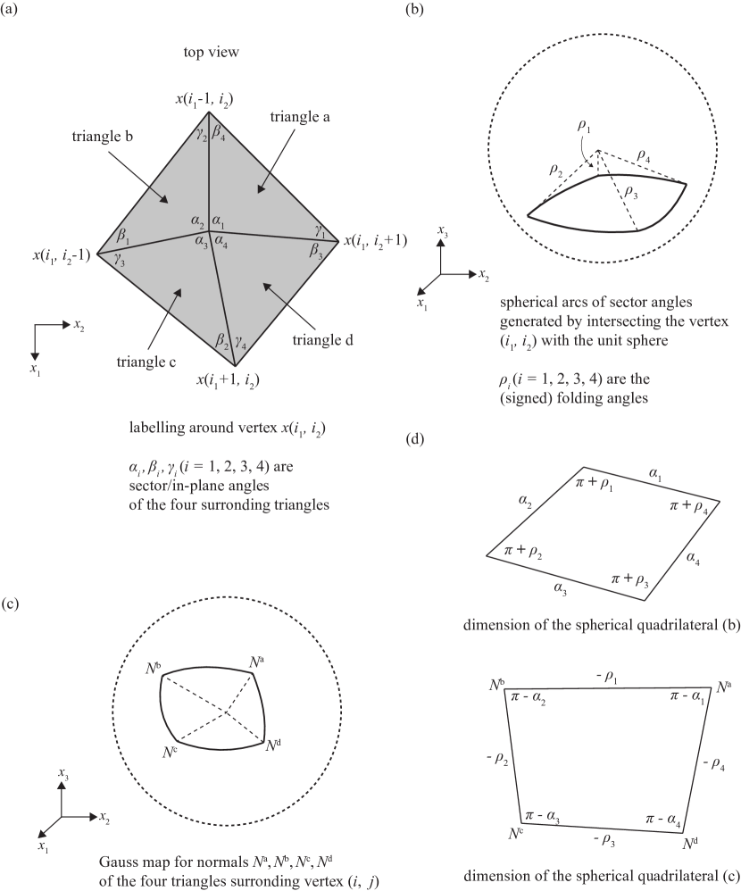
Figure 5: Labelling around vertex $x(i_{1},~{}i_{2})$ in the calculation of the discrete mean curvature vector and the discrete Gaussian curvature. Note that in (b), at each crease, a signed folding angle $\rho_{i}$ is the angle between the normal vectors of its two adjacent panels. If these two normal vectors meet on the specified side of the paper (here, upwards), $\rho_{i}\in(0,\pi)$, the crease is called a valley crease. If these two normal vectors meet on the opposite side, $\rho_{i}\in(-\pi,0)$, the crease is called a mountain crease. (b) shows four mountain creases. In (d) we could see that the two spherical quadrilaterals are dual/polar-and-poles to each other.

We will show how to use the above formula in Proposition 2 to calculate the discrete mean curvature vector $\kappa_{\mathrm{H}}N$ and the discrete Gaussian curvature $\kappa_{\mathrm{G}}$. For every $x(i),~{}i=(i_{1},~{}i_{2})\in\mathbb{Z}^{2}$ on a discrete surface, we need the information of $x(i_{1}-1,~{}i_{2})$, $x(i_{1}+1,~{}i_{2})$, $x(i_{1},~{}i_{2}-1)$ and $x(i_{1},~{}i_{2}+1)$ to calculate the area gradient of the four triangles surrounding $x(i)$. Let

$$\begin{gathered}a=x(i_{1},~{}i_{2})-x(i_{1}-1,~{}i_{2}),~{}~{}b=x(i_{1},~{}i_{2})-x(i_{1},~{}i_{2}-1)\\ c=x(i_{1},~{}i_{2})-x(i_{1}+1,~{}i_{2}),~{}~{}d=x(i_{1},~{}i_{2})-x(i_{1},~{}i_{2}+1)\end{gathered}$$

and the sum of area of the four triangles is:

$$\mathrm{area}(i) =\dfrac{1}{2}\left(\|d\times a\|+\|a\times b\|+\|b\times c\|+\|c\times d\|\right)$$

Note that the $\mathrm{area}(i)$ lives on vertex $i$. The derivative of $\mathrm{area}(i)$ with respect to $x(i)$ can be directly calculated. For example:

$$\dfrac{\mathop{}\!\mathrm{d}\|d\times a\|}{\mathop{}\!\mathrm{d}x}=\dfrac{1}{\|d\times a\|}\begin{bmatrix}(d\times a)\cdot\dfrac{\partial(d\times a)}{\partial x_{1}}\\[8.0pt] (d\times a)\cdot\dfrac{\partial(d\times a)}{\partial x_{2}}\\[8.0pt] (d\times a)\cdot\dfrac{\partial(d\times a)}{\partial x_{3}}\end{bmatrix}=\dfrac{\mathop{}\!\mathrm{d}(d\times a)}{\mathop{}\!\mathrm{d}x}\cdot\dfrac{d\times a}{\|d\times a\|}$$

and for $a=(a_{1};~{}a_{2};~{}a_{3})$ and $d=(d_{1};~{}d_{2};~{}d_{3})$:

$$\dfrac{\mathop{}\!\mathrm{d}(d\times a)}{\mathop{}\!\mathrm{d}x}=\begin{bmatrix}0&a_{3}-d_{3}&d_{2}-a_{2}\\ d_{3}-a_{3}&0&a_{1}-d_{1}\\ a_{2}-d_{2}&d_{1}-a_{1}&0\end{bmatrix}$$

Using the information above we could obtain the expression below in terms of cross product:

$$\nabla\mathrm{area}(i)= \dfrac{1}{2}\left((d-a)\times\dfrac{d\times a}{\|d\times a\|}+(a-b)\times\dfrac{a\times b}{\|a\times b\|}\right.$$

$$\left.~{}~{}+(b-c)\times\dfrac{b\times c}{\|b\times c\|}+(c-d)\times\dfrac{c\times d}{\|c\times d\|}\right)$$

Physically, $\nabla\mathrm{area}(i)$ indicates the steepest direction pulling at vertex $i$ to increase $\mathrm{area}(i)$ of the four triangles. Then apply the formula for triple cross product we will obtain the final expression, as known as the cotan formula, using the angles defined in Figure 5:

$$\nabla\mathrm{area}(i)={} \dfrac{1}{2}\left(\left(\dfrac{1}{\tan\beta_{1}}+\dfrac{1}{\tan\gamma_{1}}\right)a+\left(\dfrac{1}{\tan\beta_{2}}+\dfrac{1}{\tan\gamma_{2}}\right)b\right.$$ (32)

$$\left.~{}+\left(\dfrac{1}{\tan\beta_{3}}+\dfrac{1}{\tan\gamma_{3}}\right)c+\left(\dfrac{1}{\tan\beta_{4}}+\dfrac{1}{\tan\gamma_{4}}\right)d\right)$$

Hence the discrete mean curvature vector, i.e., the Laplace-Beltrami Operator is:

$$\begin{gathered}2\kappa_{\mathrm{H}}(i)N(i)=\dfrac{\nabla\mathrm{area}(i)}{\mathrm{area}(i)},~{}~{}\|N(i)\|=1\end{gathered}$$ (33)

Here $\kappa_{\mathrm{H}}(i)$ and $N(i)$ both live on vertex $i$. Note that if $\nabla\mathrm{area}(i)=0$, for example when the five points in Figure 5 are coplanar, we take $N(i)$ as the average of the surrounding normal vectors.

Next, we can calculate the normal of the surrounding four triangles, whose spherical view is provided in Figure 5(c)

$$\begin{gathered}N^{\mathrm{a}}=\dfrac{d\times a}{\|d\|\|a\|\sin\alpha_{1}},~{}~{}N^{\mathrm{b}}=\dfrac{a\times b}{\|a\|\|b\|\sin\alpha_{2}}\\ N^{\mathrm{c}}=\dfrac{b\times c}{\|b\|\|c\|\sin\alpha_{3}},~{}~{}N^{\mathrm{d}}=\dfrac{c\times d}{\|c\|\|d\|\sin\alpha_{4}}\end{gathered}$$

$$\begin{gathered}N^{\mathrm{a}}\cdot N^{\mathrm{b}}=\cos\rho_{1},~{}~{}N^{\mathrm{b}}\cdot N^{\mathrm{c}}=\cos\rho_{2}\\ N^{\mathrm{c}}\cdot N^{\mathrm{d}}=\cos\rho_{3},~{}~{}N^{\mathrm{d}}\cdot N^{\mathrm{a}}=\cos\rho_{4}\end{gathered}$$

Note that the Gauss map is an involution (a mapping is its inverse) of the direction vectors along $a$, $b$, $c$, $d$.

$$\begin{gathered}\dfrac{a}{\|a\|}=-\dfrac{N^{\mathrm{a}}\times N^{\mathrm{b}}}{\sin\rho_{1}},~{}~{}\dfrac{b}{\|b\|}=-\dfrac{N^{\mathrm{b}}\times N^{\mathrm{c}}}{\sin\rho_{2}}\\ \dfrac{c}{\|c\|}=-\dfrac{N^{\mathrm{c}}\times N^{\mathrm{d}}}{\sin\rho_{3}},~{}~{}\dfrac{d}{\|d\|}=-\dfrac{N^{\mathrm{d}}\times N^{\mathrm{a}}}{\sin\rho_{4}}\end{gathered}$$

The geometrical reason is $a$ being orthogonal to both $N^{\mathrm{a}}$ and $N^{\mathrm{b}}$. The same principle holds for the rest.

An important fact from spherical trigonometry is that the spherical linkage sharing identical motion with the degree-4 vertex shown in Figure 5(b) is the polar quadrilateral of the spherical quadrilateral formed by the Gauss map shown in Figure 5(c). The sector angles and folding angles are therefore related as indicated in Figure 5(d). Further, the area of a spherical quadrilateral is the sum of interior angles minus $2\pi$ (also called the angular defect), which leads to the calculation of discrete Gaussian curvature:

$$\kappa_{\mathrm{G}}(i)=2\pi-\alpha_{1}-\alpha_{2}-\alpha_{3}-\alpha_{4}$$ (34)

$\kappa_{\mathrm{G}}(i)$ also lives on vertex $i$.

The above calculation method of the discrete mean and Gaussian curvature is just one of the admissible definitions. In practice the calculation might be altered for different discrete surfaces, for example, Meyer et al. (2003) and the edge-constrained net introduced in Hoffmann et al. (2017).

Appendix E Discrete nets

This section will introduce the discrete analogue of coordinate nets derived in Section B. Here ‘discrete analogue’ means the discrete system (usually a partial difference system) defined by a discrete coordinate net is a discretization of a smooth system (usually a partial differential system). We will show the conversion between the smooth and discrete notations by examining multiple discrete nets in line with the smooth nets provided in Section B and from the discussion on convergence in Section G. It is worth mentioning that there may be multiple approaches to discretize a smooth net, and the choice of discrete net will depend on specific scenarios and requirements (for example, in the simulation of isometric deformation). The labelling of geometrical quantities on a discrete net is provided in Figure 6.

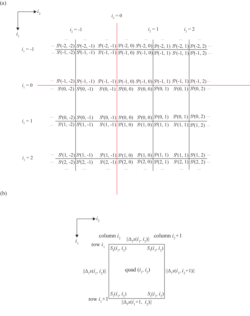
Figure 6: Labelling of vertices, lengths and angles of a discrete net. Note that these figures are not a three-dimensional drawing, and $x(i_{1},~{}i_{2}),~{}x(i_{1}+1,~{}i_{2}),~{}x(i_{1}+1,~{}i_{2}+1),~{}x(i_{1},~{}i_{2}+1)$ are not necessarily planar. The sector angles are $S^{\mathrm{a}}(i),~{}S^{\mathrm{b}}(i),~{}S^{\mathrm{c}}(i),~{}S^{\mathrm{d}}(i),~{}i=(i_{1},~{}i_{2})\in\mathbb{Z}^{2}$. The crease lengths are $\|\triangle_{1}x(i)\|=\|x(i_{1}+1,~{}i_{2})-x(i_{1},~{}i_{2})\|,~{}\|\triangle_{2}x(i)\|=\|x(i_{1},~{}i_{2}+1)-x(i_{1},~{}i_{2})\|,~{}i=(i_{1},~{}i_{2})\in\mathbb{Z}^{2}$.

A discrete surface $X:\mathbb{Z}^{2}\rightarrow\mathbb{R}^{3}$ is called a discrete Chebyshev net if

$$\triangle_{2}\|\triangle_{1}x\|^{2}=\triangle_{1}\|\triangle_{2}x\|^{2}=0,~{}~{}\mathrm{for~{}all~{}}i=(i_{1},~{}i_{2})\in\mathbb{Z}^{2}$$ (35)

The discrete operators are in the form of:

$$\begin{gathered}\triangle_{1}x(i)=x(i_{1}+1,~{}i_{2})-x(i_{1},~{}i_{2})\\ \triangle_{2}x(i)=x(i_{1},~{}i_{2}+1)-x(i_{1},~{}i_{2})\\ \triangle_{1}\triangle_{2}x(i)=\triangle_{2}\triangle_{1}x(i)=x(i_{1}+1,~{}i_{2}+1)-x(i_{1},~{}i_{2}+1)-x(i_{1}+1,~{}i_{2})+x(i_{1},~{}i_{2})\end{gathered}$$

Note that $\triangle_{1}x$ lives on grid lines $i_{2}$, $\triangle_{2}x$ lives on grid lines $i_{1}$, $\triangle_{1}\triangle_{2}x$ lives on quadrilaterals $(i_{1},~{}i_{2})$.

$$\triangle_{2}\|\triangle_{1}x\|^{2} =\|\triangle_{1}x(i_{1},~{}i_{2}+1)\|^{2}-\|\triangle_{1}x(i_{1},~{}i_{2})\|^{2}$$

$$=\|x(i_{1}+1,~{}i_{2}+1)-x(i_{1},~{}i_{2}+1)\|^{2}-\|x(i_{1}+1,~{}i_{2})-x(i_{1},~{}i_{2})\|^{2}$$

$$=\triangle_{1}\triangle_{2}x(i)\cdot(x(i_{1}+1,~{}i_{2}+1)-x(i_{1},~{}i_{2}+1)+x(i_{1}+1,~{}i_{2})-x(i_{1},~{}i_{2}))$$

$$\triangle_{1}\|\triangle_{2}x\|^{2} =\|\triangle_{2}x(i_{1}+1,~{}i_{2})\|^{2}-\|\triangle_{2}x(i_{1},~{}i_{2})\|^{2}$$

$$=\|x(i_{1}+1,~{}i_{2}+1)-x(i_{1}+1,~{}i_{2})\|^{2}-\|x(i_{1},~{}i_{2}+1)-x(i_{1},~{}i_{2})\|^{2}$$

$$=\triangle_{1}\triangle_{2}x(i)\cdot(x(i_{1}+1,~{}i_{2}+1)+x(i_{1},~{}i_{2}+1)-x(i_{1}+1,~{}i_{2})-x(i_{1},~{}i_{2}))$$

Hence the partial difference equation for a discrete Chebyshev net, Eq. (35), is equivalent to

$$\begin{dcases}\triangle_{1}\triangle_{2}x(i)\cdot(x(i_{1}+1,~{}i_{2}+1)-x(i_{1},~{}i_{2}))=0\\ \triangle_{1}\triangle_{2}x(i)\cdot(x(i_{1},~{}i_{2}+1)-x(i_{1}+1,~{}i_{2}))=0\end{dcases}$$ (36)

$$~{}~{}\Leftrightarrow \begin{dcases}\triangle_{1}\triangle_{2}x(i)=\dfrac{\lambda(i)}{2}(x(i_{1}+1,~{}i_{2}+1)-x(i_{1},~{}i_{2}))\times(x(i_{1},~{}i_{2}+1)-x(i_{1}+1,~{}i_{2}))\\ \lambda:\mathbb{Z}^{2}\rightarrow\mathbb{R}\mathrm{~{}living~{}on~{}quadrilaterals~{}}(i_{1},~{}i_{2})\end{dcases}$$

The reason for choosing $\lambda/2$ is for the consistency with its smooth analogue, Eq. (11). It can be verified that on the integer grid, if seeing $u_{1}$ in the direction along $(\sqrt{2}/2,~{}\sqrt{2}/2)$, and seeing $u_{2}$ in the direction along $(-\sqrt{2}/2,~{}\sqrt{2}/2)$, we have

$$\begin{gathered}\triangle_{1}\triangle_{2}x\sim\dfrac{\partial^{2}x}{\partial u_{1}\partial u_{2}}\\ x(i_{1}+1,~{}i_{2}+1)-x(i_{1},~{}i_{2})\sim\sqrt{2}\dfrac{\partial x}{\partial u_{1}}\\ x(i_{1},~{}i_{2}+1)-x(i_{1}+1,~{}i_{2})\sim\sqrt{2}\dfrac{\partial x}{\partial u_{2}}\end{gathered}$$

hence the amplitude $\lambda$ has the same meaning for both the discrete and smooth case.

When $\triangle_{1}\triangle_{2}x\neq 0$, see Figure 7(a) for a geometric illustration for a Chebyshev quadrilateral. Apply a parallel transport from $BD$ to $B^{\prime}D^{\prime}$ such that the intersection $O^{\prime}$ of $AC$ and $B^{\prime}D^{\prime}$ bisects both $AC$ and $B^{\prime}D^{\prime}$. The side length condition $AB=CD$, $AD=BC$ implies that both $BB^{\prime}$ and $DD^{\prime}$ are perpendicular to the planar parallelogram $AB^{\prime}CD^{\prime}$, and we could see that $BB^{\prime}=DD^{\prime}=OO^{\prime}=\triangle_{1}\triangle_{2}x/2$. When $\triangle_{1}\triangle_{2}x=0$, as shown in Figure 7(b), $ABCD$ becomes a planar parallelogram, geometrically flipping $D$ to the other side of plane $AB^{\prime}CD^{\prime}$.

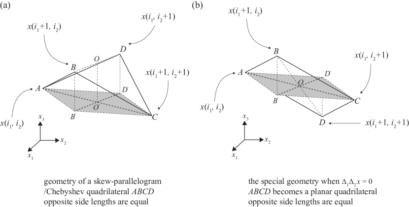
Figure 7: (a) A figure illustrating the geometry of a skew-parallelogram/Chebyshev quadrilateral, where the side lengths $AB=CD$, $AD=BC$. (b) Degeneration to a planar quadrilateral when $\triangle_{1}\triangle_{2}x=0$. In both figures, $A,~{}B,~{}C,~{}D$ refer to the position of $x(i_{1},~{}i_{2}),~{}x(i_{1}+1,~{}i_{2}),~{}x(i_{1}+1,~{}i_{2}+1),~{}x(i_{1},~{}i_{2}+1)$.

We could see that one reasonable way to define the discrete normal field is to define $N(i),~{}i=(i_{1},~{}i_{2})\in\mathbb{Z}^{2}$ on each quadrilateral $(i_{1},~{}i_{2})$, along the direction of $O^{\prime}O$:

$$N(i)=\dfrac{(x(i_{1}+1,~{}i_{2}+1)-x(i_{1},~{}i_{2}))\times(x(i_{1},~{}i_{2}+1)-x(i_{1}+1,~{}i_{2}))}{\|(x(i_{1}+1,~{}i_{2}+1)-x(i_{1},~{}i_{2}))\times(x(i_{1},~{}i_{2}+1)-x(i_{1}+1,~{}i_{2}))\|}$$ (37)

Additionally, $\lambda(i),~{}i=(i_{1},~{}i_{2})\in\mathbb{Z}^{2}$ for a discrete Chebyshev net shows the ‘curvature’ of a Chebyshev quadrilateral since

$$\lambda(i) =\dfrac{\triangle_{1}\triangle_{2}x(i)\cdot N(i)}{\|(x(i_{1}+1,~{}i_{2}+1)-x(i_{1},~{}i_{2}))\times(x(i_{1},~{}i_{2}+1)-x(i_{1}+1,~{}i_{2}))\|}$$

$$=\dfrac{2\mathrm{length}(OO^{\prime})}{\mathrm{area}(AB^{\prime}CD^{\prime})}$$

Note that the smooth analogue of $\lambda$ for a Chebyshev net is provided in Eq. (12). The above information for a discrete Chebyshev net is from Schief (2007).

A discrete orthogonal Chebyshev net is a discrete Chebyshev net where $x(i_{1}+1,~{}i_{2}+1)-x(i_{1},~{}i_{2})$ is perpendicular to $x(i_{1},~{}i_{2}+1)-x(i_{1}+1,~{}i_{2})$ for all $i\in\mathbb{Z}^{2}$. It implies that the length of the four sides of the Chebyshev quadrilateral is equal, i.e. $AB=BC=CD=DA$ in Figure 7. Such net in fact has a cylindrical shape.

A discrete surface $X:\mathbb{Z}^{2}\rightarrow\mathbb{R}^{3}$ is called a discrete asymptotic net if:

$$\begin{dcases}\triangle_{1}^{2}x(i)\cdot N(i)=0\\ \triangle_{2}^{2}x(i)\cdot N(i)=0\end{dcases},\mathrm{~{}~{}for~{}all~{}}i=(i_{1},~{}i_{2})\in\mathbb{Z}^{2}$$

where

$$\begin{gathered}\triangle_{1}^{2}x(i)=x(i_{1}-1,~{}i_{2})+x(i_{1}+1,~{}i_{2})-2x(i_{1},~{}i_{2})\\ \triangle_{2}^{2}x(i)=x(i_{1},~{}i_{2}-1)+x(i_{1},~{}i_{2}+1)-2x(i_{1},~{}i_{2})\end{gathered}$$

From Eq. (33):

$$\nabla\mathrm{area}(i)={} \dfrac{1}{2}\left(\left(\dfrac{1}{\tan\beta_{1}}+\dfrac{1}{\tan\gamma_{1}}\right)(x(i_{1},~{}i_{2})-x(i_{1}-1,~{}i_{2}))\right.$$

$$~{}~{}+\left(\dfrac{1}{\tan\beta_{2}}+\dfrac{1}{\tan\gamma_{2}}\right)(x(i_{1},~{}i_{2})-x(i_{1},~{}i_{2}-1))$$

$$~{}~{}+\left(\dfrac{1}{\tan\beta_{3}}+\dfrac{1}{\tan\gamma_{3}}\right)(x(i_{1},~{}i_{2})-x(i_{1}+1,~{}i_{2}))$$

$$~{}~{}+\left.\left(\dfrac{1}{\tan\beta_{4}}+\dfrac{1}{\tan\gamma_{4}}\right)(x(i_{1},~{}i_{2})-x(i_{1},~{}i_{2}+1))\right)$$

From direct calculation we could see that the condition for a discrete asymptotic net is that $x(i_{1},~{}i_{2}),~{}x(i_{1},~{}i_{2}-1),~{}x(i_{1}+1,~{}i_{2}),~{}x(i_{1},~{}i_{2}+1),~{}x(i_{1}-1,~{}i_{2})$ are coplanar, then $N(i)$ is perpendicular to this plane and hence perpendicular to both $\triangle_{1}^{2}x(i)$ and $\triangle_{2}^{2}x(i)$. The above geometry also indicates that both $N(i_{1},~{}i_{2})$ and $N(i_{1}+1,~{}i_{2})$ are perpendicular to $\triangle_{1}x$; and both $N(i_{1},~{}i_{2})$ and $N(i_{1},~{}i_{2}+1)$ are perpendicular to $\triangle_{2}x$. The Lelieuvre normal field for an asymptotic net is defined as $N^{\mathrm{L}}=N(-\kappa_{\mathrm{G}})^{-1/4}$ (one option for discrete Gaussian curvature is the angular defect Eq. (34)), and we could define the discrete Lelieuvre normal field $N^{\mathrm{L}}(i_{1},~{}i_{2})$ to be a suitable scaling of $N(i_{1},~{}i_{2})$ such that:

$$\begin{dcases}N^{\mathrm{L}}\times\triangle_{1}N^{\mathrm{L}}=\triangle_{1}x\\ \triangle_{2}N^{\mathrm{L}}\times N^{\mathrm{L}}=\triangle_{2}x\end{dcases}$$ (38)

From

$$\begin{gathered}N^{\mathrm{L}}(i_{1},~{}i_{2})\times N^{\mathrm{L}}(i_{1}+1,~{}i_{2})=x(i_{1}+1,~{}i_{2})-x(i_{1},~{}i_{2})\\ N^{\mathrm{L}}(i_{1},~{}i_{2}+1)\times N^{\mathrm{L}}(i_{1}+1,~{}i_{2}+1)=x(i_{1}+1,~{}i_{2}+1)-x(i_{1},~{}i_{2}+1)\\ N^{\mathrm{L}}(i_{1},~{}i_{2}+1)\times N^{\mathrm{L}}(i_{1},~{}i_{2})=x(i_{1},~{}i_{2}+1)-x(i_{1},~{}i_{2})\\ N^{\mathrm{L}}(i_{1}+1,~{}i_{2}+1)\times N^{\mathrm{L}}(i_{1}+1,~{}i_{2})=x(i_{1}+1,~{}i_{2}+1)-x(i_{1}+1,~{}i_{2})\\ \end{gathered}$$ (39)

sum the equations above we could see that:

$$(N^{\mathrm{L}}(i_{1},~{}i_{2})+N^{\mathrm{L}}(i_{1}+1,~{}i_{2}+1))\times(N^{\mathrm{L}}(i_{1}+1,~{}i_{2})+N^{\mathrm{L}}(i_{1},~{}i_{2}+1))=0$$

which is equivalent to the discrete Moutard Equation for $N^{\mathrm{L}}$:

$$\begin{gathered}\triangle_{1}\triangle_{2}N^{\mathrm{L}}=\dfrac{\lambda(i_{1},~{}i_{2})}{2}(N^{\mathrm{L}}(i_{1}+1,~{}i_{2})+N^{\mathrm{L}}(i_{1},~{}i_{2}+1)),~{}~{}\lambda:\mathbb{Z}^{2}\rightarrow\mathbb{R}\end{gathered}$$ (40)

The reason for choosing $\lambda/2$ is for the consistency with its smooth analogue, Eq. (20).

A discrete surface $X:\mathbb{Z}^{2}\rightarrow\mathbb{R}^{3}$ is called a discrete asymptotic Chebyshev net, as known as a K-hedron/discrete K-surface in previous literatures if both Eq. (35) and the five points coplanar condition are satisfied. In Figure 7(a), set vector $O^{\prime}B^{\prime}=a$, vector $O^{\prime}C=b$, vector $O^{\prime}O=c$. Here $c$ is perpendicular to both $a$ and $b$. These three vectors determine the shape of a Chebyshev quadrilateral. Since vector $AB=a+b+c$, vector $BC=-a+b-c$, vector $CD=-a-b+c$, vector $DA=a-b-c$, let

$$\begin{gathered}N^{\mathrm{L}}(i_{1},~{}i_{2})=\dfrac{a\times(b+c)}{\sqrt{(a\times b)\cdot c}}\\ N^{\mathrm{L}}(i_{1}+1,~{}i_{2})=\dfrac{b\times(a+c)}{\sqrt{(a\times b)\cdot c}}\\ N^{\mathrm{L}}(i_{1}+1,~{}i_{2}+1)=\dfrac{a\times(b-c)}{\sqrt{(a\times b)\cdot c}}\\ N^{\mathrm{L}}(i_{1},~{}i_{2}+1)=\dfrac{b\times(a-c)}{\sqrt{(a\times b)\cdot c}}\\ \end{gathered}$$

we could examine that $N^{\mathrm{L}}$ is a discrete Lelieuvre normal field, which agrees with Eq. (39):

$$\begin{gathered}N^{\mathrm{L}}(i_{1},~{}i_{2})\times N^{\mathrm{L}}(i_{1}+1,~{}i_{2})=a+b+c\\ N^{\mathrm{L}}(i_{1},~{}i_{2}+1)\times N^{\mathrm{L}}(i_{1}+1,~{}i_{2}+1)=a+b-c\\ N^{\mathrm{L}}(i_{1},~{}i_{2}+1)\times N^{\mathrm{L}}(i_{1},~{}i_{2})=-a+b+c\\ N^{\mathrm{L}}(i_{1}+1,~{}i_{2}+1)\times N^{\mathrm{L}}(i_{1}+1,~{}i_{2})=-a+b-c\\ \end{gathered}$$

It turns out that in the discrete Moutard Equation for a K-hedron, $\lambda(i_{1},~{}i_{2})=-4$,

$$\begin{gathered}\triangle_{1}\triangle_{2}N^{\mathrm{L}}=-2(N^{\mathrm{L}}(i_{1}+1,~{}i_{2})+N^{\mathrm{L}}(i_{1},~{}i_{2}+1))\end{gathered}$$ (41)

In terms of the discrete normal field:

$$\begin{gathered}N(i_{1},~{}i_{2})=\dfrac{a\times(b+c)}{\|a\times(b+c)\|},~{}~{}N(i_{1}+1,~{}i_{2})=\dfrac{b\times(a+c)}{\|b\times(a+c)\|}\\ N(i_{1}+1,~{}i_{2}+1)=\dfrac{a\times(b-c)}{\|a\times(b-c)\|},~{}~{}N(i_{1},~{}i_{2}+1)=\dfrac{b\times(a-c)}{\|b\times(a-c)\|}\\ \end{gathered}$$

From the geometry illustrated in Figure 7(a):

$$\|a\times(b+c)\|=\|a\times(b-c)\|,~{}~{}\|b\times(a+c)\|=\|b\times(a-c)\|$$

$$\begin{gathered}\triangle_{1}\triangle_{2}N=2\left(\dfrac{1}{\|a\times(b+c)\|}+\dfrac{1}{\|b\times(a+c)\|}\right)a\times b\\ \triangle_{1}\triangle_{2}N=-\left(\dfrac{\|b\times(a+c)\|}{\|a\times(b+c)\|}+1\right)(N(i_{1}+1,~{}i_{2})+N(i_{1},~{}i_{2}+1))\end{gathered}$$

$$\begin{gathered}N(i_{1}+1,~{}i_{2}+1)-N(i_{1},~{}i_{2})=\dfrac{2c\times a}{\|a\times(b+c)\|}\\ N(i_{1},~{}i_{2}+1)-N(i_{1}+1,~{}i_{2})=\dfrac{2c\times b}{\|b\times(a+c)\|}\end{gathered}$$

$$\begin{gathered}\triangle_{1}\triangle_{2}N\cdot(N(i_{1}+1,~{}i_{2}+1)-N(i_{1},~{}i_{2}))=0\\ \triangle_{1}\triangle_{2}N\cdot(N(i_{1},~{}i_{2}+1)-N(i_{1}+1,~{}i_{2}))=0\end{gathered}$$

The above derivation leads to the following proposition, which is parallel to its smooth analogue:

Proposition 3.

The Gauss map of a discrete K-surface is a discrete Chebyshev net. A discrete K-surface is the only discrete asymptotic net with a discrete Chebyshev Gauss map.

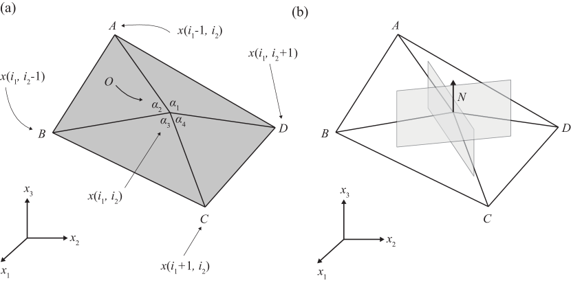
Figure 8: A figure illustrating the geometry of a discrete geodesic net, where opposite sector angles at each interior vertex are equal. One important geometrical feature is the coordinate curve normals are identical to the surface normal at every interior vertex.

A discrete surface $X:\mathbb{Z}^{2}\rightarrow\mathbb{R}^{3}$ is called a discrete geodesic net if opposite sector angles at every vertex are equal:

$$\begin{dcases}S_{1}(i_{1},~{}i_{2}+1)=S_{3}(i_{1}+1,~{}i_{2})\\ S_{2}(i_{1},~{}i_{2})=S_{4}(i_{1}+1,~{}i_{2}+1)\end{dcases}\textrm{~{}~{}~{}for~{}all~{}}i\in\mathbb{Z}^{2}$$

which means $\alpha_{1}=\alpha_{3},~{}\alpha_{2}=\alpha_{4}$ in Figure 8.

A discrete surface $X:\mathbb{Z}^{2}\rightarrow\mathbb{R}^{3}$ is called a discrete orthogonal geodesic net if all four sector angles at every vertex are equal:

$$S_{1}(i_{1},~{}i_{2}+1)=S_{2}(i_{1},~{}i_{2})=S_{3}(i_{1}+1,~{}i_{2})=S_{4}(i_{1}+1,~{}i_{2}+1)\textrm{~{}~{}~{}for~{}all~{}}i\in\mathbb{Z}^{2}$$

which means $\alpha_{1}=\alpha_{2}=\alpha_{3}=\alpha_{4}$ in Figure 8.

A geodesic curve is ‘as straight as possible’ and has ‘no lateral acceleration’ on a surface. By requiring $\alpha_{1}+\alpha_{2}=\alpha_{3}+\alpha_{4}$ and $\alpha_{2}+\alpha_{3}=\alpha_{4}+\alpha_{1}$, the polylines $AOC$ and $BOD$ will divide the angular defect $\kappa_{\mathrm{G}}=2\pi-\alpha_{1}-\alpha_{2}-\alpha_{3}-\alpha_{4}$ equally. This leads to the angle condition for a discrete geodesic net mentioned above.

Next we will calculate the normal vector defined on $x(i)$, let $a,~{}b,~{}c,~{}d$ be the direction vector of $OA,~{}OB,~{}OC,~{}OD$:

$$\begin{gathered}a=\dfrac{x(i_{1},~{}i_{2})-x(i_{1}-1,~{}i_{2})}{\|x(i_{1},~{}i_{2})-x(i_{1}-1,~{}i_{2})\|},~{}~{}b=\dfrac{x(i_{1},~{}i_{2})-x(i_{1},~{}i_{2}-1)}{\|x(i_{1},~{}i_{2})-x(i_{1},~{}i_{2}-1)\|}\\ c=\dfrac{x(i_{1},~{}i_{2})-x(i_{1}+1,~{}i_{2})}{\|x(i_{1},~{}i_{2})-x(i_{1}+1,~{}i_{2})\|},~{}~{}d=\dfrac{x(i_{1},~{}i_{2})-x(i_{1},~{}i_{2}+1)}{\|x(i_{1},~{}i_{2})-x(i_{1},~{}i_{2}+1)\|}\end{gathered}$$

Along the $i_{1}$ direction, the discrete Frenet-Serret frame is

$$\boldsymbol{x}_{\mathrm{t}}^{1}=-\dfrac{a-c}{\|a-c\|},~{}~{}\boldsymbol{x}_{\mathrm{n}}^{1}=-\dfrac{a+c}{\|a+c\|},~{}~{}\boldsymbol{x}_{\mathrm{b}}^{1}=\boldsymbol{x}_{\mathrm{t}}^{1}\times\boldsymbol{x}_{\mathrm{n}}^{1}$$

Along the $i_{2}$ direction, the discrete Frenet-Serret frame is

$$\boldsymbol{x}_{\mathrm{t}}^{2}=-\dfrac{b-d}{\|b-d\|},~{}~{}\boldsymbol{x}_{\mathrm{n}}^{2}=-\dfrac{b+d}{\|b+d\|},~{}~{}\boldsymbol{x}_{\mathrm{b}}^{2}=\boldsymbol{x}_{\mathrm{t}}^{2}\times\boldsymbol{x}_{\mathrm{n}}^{2}$$

The normal vector is:

$$N(i)=\dfrac{\boldsymbol{x}_{\mathrm{t}}^{1}\times\boldsymbol{x}_{\mathrm{t}}^{2}}{\|\boldsymbol{x}_{\mathrm{t}}^{1}\times\boldsymbol{x}_{\mathrm{t}}^{2}\|}$$

Since opposite sector angles are equal, $\boldsymbol{x}_{\mathrm{n}}^{1}\cdot\boldsymbol{x}_{\mathrm{t}}^{2}=0$ and $\boldsymbol{x}_{\mathrm{n}}^{2}\cdot\boldsymbol{x}_{\mathrm{t}}^{1}=0$. We could see that either $\boldsymbol{x}_{\mathrm{n}}^{1}$ or $\boldsymbol{x}_{\mathrm{n}}^{2}$ is perpendicular to both $\boldsymbol{x}_{\mathrm{t}}^{1}$ and $\boldsymbol{x}_{\mathrm{t}}^{2}$, hence

$$N(i)=\boldsymbol{x}_{\mathrm{n}}^{1}=\boldsymbol{x}_{\mathrm{n}}^{2}$$

The above equality of normal vectors further shows that polylines $AOC$ and $BOD$ are discrete analogue of geodesic curves on a surface.

For a discrete orthogonal geodesic net, we further have $\boldsymbol{x}_{\mathrm{t}}^{1}$ perpendicular to $\boldsymbol{x}_{\mathrm{t}}^{2}$, which geometrically explains that the coordinate curves are perpendicular at every interior vertex. The information of discrete geodesic net and discrete orthogonal geodesic net is from Rabinovich et al. (2018).

A discrete surface $X:\mathbb{Z}^{2}\rightarrow\mathbb{R}^{3}$ is called a discrete conjugate net if all its elementary quadrilaterals formed by $x(i_{1},~{}i_{2}),~{}x(i_{1}+1,~{}i_{2}),~{}x(i_{1}+1,~{}i_{2}+1),~{}x(i_{1},~{}i_{2}+1)$ are planar for all $i\in\mathbb{Z}$. Here the normal vector $N(i)$ at each vertex is associated with the normal vector of the above planar quadrilateral and hence $\triangle_{1}\triangle_{2}x$ is perpendicular to $N$. Using the Christoffel symbol, the planarity condition for a discrete conjugate net is equivalent to:

$$\triangle_{1}\triangle_{2}x=\Gamma_{12}^{1}\triangle_{1}x+\Gamma_{12}^{2}\triangle_{2}x,~{}~{}\Gamma_{12}^{1},~{}\Gamma_{12}^{2}:\mathbb{Z}^{2}\rightarrow\mathbb{R}$$ (42)

Here $\Gamma_{12}^{1}(i)$, $\Gamma_{12}^{2}(i)$ can be directly calculated as the coefficients of the above linear combination for the given discrete net $x$. The smooth analogue of $\Gamma_{12}^{1}(i)$, $\Gamma_{12}^{2}(i)$ is the corresponding Christoffel symbol $\Gamma_{12}^{1},~{}\Gamma_{12}^{2}$ for the corresponding conjugate net.

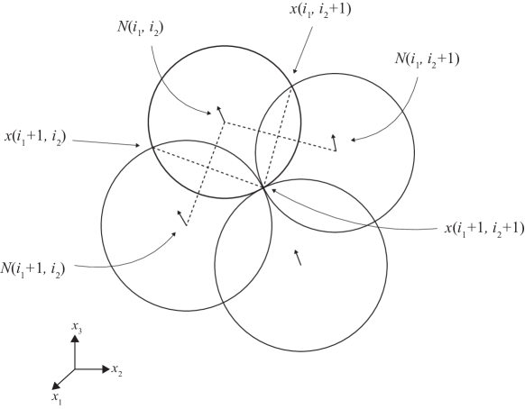
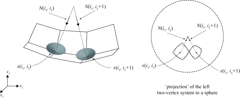
Figure 9: Illustration of the geometry of a circular net, where $x(i_{1},~{}i_{2}),~{}x(i_{1}+1,~{}i_{2}),~{}x(i_{1}+1,~{}i_{2}+1),~{}x(i_{1},~{}i_{2}+1)$ are concircular for all $i\in\mathbb{Z}^{2}$. Here we draw a special case where pairs of circles located diagonally from each other are tangent. It happens, for example, on a discrete isothermic net whose cross ratio is limited to -1.

Figure 10: Illustration of the geometry of a conical net, where the four planar quadrilaterals incident to a vertex are tangent to a common cone whose apex is the vertex. For every pair of adjacent cones, there exists a sphere that touches both at the apexes. The centre of this sphere is the intersection point of the cones’ axes.

A discrete conjugate net $X:\mathbb{Z}^{2}\rightarrow\mathbb{R}^{3}$ is called a circular net if all its elementary quadrilaterals formed by $x(i_{1},~{}i_{2}),~{}x(i_{1}+1,~{}i_{2}),~{}x(i_{1}+1,~{}i_{2}+1),~{}x(i_{1},~{}i_{2}+1)$ have circumscribed circles, in other words, they are concircular. It is one of the common discrete analogue of the curvature line net. From Figure 10, $\triangle_{2}x(i_{1}+1,~{}i_{2})$ is perpendicular to both $N(i_{1},~{}i_{2})$ and $N(i_{1}+1,~{}i_{2})$, hence perpendicular to $\triangle_{1}N(i_{1},~{}i_{2})$; $\triangle_{1}x(i_{1},~{}i_{2}+1)$ is perpendicular to both $N(i_{1},~{}i_{2})$ and $N(i_{1},~{}i_{2}+1)$, hence perpendicular to $\triangle_{2}N(i_{1},~{}i_{2})$. This relation forms the discrete analogue of a curvature line net, Eq. (28).

A discrete conjugate net $X:\mathbb{Z}^{2}\rightarrow\mathbb{R}^{3}$ is called a conical net if the four planar quadrilaterals incident to a vertex are tangent to a common cone whose apex is the vertex. The discrete normal vector $N(i)$ assigned to each vertex $i$ is along the axis of the cone, see Figure 10(a). A conical net is another common discrete analogue of the curvature line net. We can interpret it by drawing the corresponding spherical 4-bar linkages of the degree-4 two-vertex system on a sphere. The cones become inscribed circles of the two spherical quadrilaterals, whose axes intersect at the centre of the sphere. We could see that $\triangle_{2}x(i_{1},~{}i_{2})$ is parallel to $\triangle_{2}N(i_{1},~{}i_{2})$, similarly, $\triangle_{1}x(i_{1},~{}i_{2})$ is parallel to $\triangle_{1}N(i_{1},~{}i_{2})$. This relation forms the discrete analogue of a curvature line net, Eq. (28).

Proposition 4.

Properties of a conical net:

1. (Wang et al., 2007) The sum of opposite sector angles of each vertex are equal.

2. (Bobenko and Suris, 2008, Section 3.4) A discrete conjugate net $X$ is a conical net if and only if the Gauss map is a circular net. A discrete conjugate net $X$ is a circular net if and only if the Gauss map is a conical net.

Regarding [1], intuitively, as shown in Figure 10, the sum of the length of opposite spherical arcs are equal if the spherical quadrilateral admits an inscribed circle. Regarding [2], at every vertex, the angles between all four normal vectors and the axis of the cone are equal, therefore the tips of these normal vectors are concircular, and the centre of this circle is on the axis of the cone.

Appendix F Initial condition for discrete nets

The various discrete nets introduced in Section E are solutions of parametric partial difference equations. In this section we will focus on the well-posedness for such a discrete system. Similarly, we hope a given initial condition leads to a unique solution, which smoothly relies on the initial value and parameter.

In parallel with Section C, we will focus on a first-order partial difference system for $x(i)$:

$$\triangle x=f(x;~{}b)~{}~{}\Leftrightarrow~{}~{}\triangle_{k}x_{j}=f_{jk}(x;~{}b)$$

where $i\in\mathbb{Z}^{m}$; $x\in\mathbb{R}^{n}~{}(m,~{}n\in\mathbb{Z}_{+})$; $f\in\mathbb{R}^{n\times m}$ is a matrix of smooth functions, $b\in\mathbb{R}^{p}~{}(p\in\mathbb{Z}_{+})$ are the $p$ parameters for the system. Similar to Section C, we further require $f$ and all the partial derivatives of $f$ are bounded and possess a global Lipschitz constant. Consequently no blow-ups (value goes to infinity) are possible and hence the well-posedness can be continued to the boundary of $I^{m}$. If there are higher order partial differences, we could try transferring the system to first-order by adding the number of variables. For example, when $\triangle_{1}\triangle_{2}x=x,~{}x\in\mathbb{R}$, we could set $y(i)=\triangle_{1}x$ and $z(i)=\triangle_{2}x$, so that $(x,~{}y,~{}z)$ forms an equivalent first-order system with compatibility condition $\triangle_{2}y=\triangle_{1}z$.

The definitions for the evolution direction, stationary direction, initial value and well-posedness for a first-order partial difference system are verbatim repetition for those defined for a partial differential system in Section C. For each discrete net introduced in Section E, we will introduce the construction method leading to a unique configuration from the initial condition. It could be directly examined that solution smoothly relies on the initial value and parameter.

Discrete Chebyshev net

Initial value

Two discrete coordinate curves $x(i_{1},~{}0)$ and $x(0,~{}i_{2})$ intersecting at $x(0,~{}0)$.

Parameter

The ratio $\lambda$ in Eq. (36) for all quadrilaterals $(i_{1},~{}i_{2})$.

Step a

In the quadrant $\mathbb{Z}_{+}^{2}$, recursively calculate $x(i_{1}+1,~{}i_{2}+1)$ from $x(i_{1},~{}i_{2})$, $x(i_{1}+1,~{}i_{2})$, $x(i_{1},~{}i_{2}+1)$ using Eq. (36). Geometrically in Figure 7(a), when points $A,~{}B,~{}C$ are fixed, the shape of the Chebyshev quadrilateral can be controlled by the length of $BB^{\prime}$, or equivalently $\lambda$.

Step b

Use the same method described in Step a to calculate the other three quadrants to obtain the entire mesh.

Regularity condition

Every step returns a non-degenerated and bounded result.

Discrete orthogonal Chebyshev net

Initial value

Two discrete coordinate curves $x(i_{1},~{}0)$ and $x(0,~{}i_{2})$ intersecting at $x(0,~{}0)$ where $\|\triangle_{1}x(i_{1},~{}0)\|=\|\triangle_{1}x(i_{1}+1,~{}0)\|=\|\triangle_{2}x(0,~{}i_{2})\|=\|\triangle_{2}x(0,~{}i_{2}+1)\|$ for all $i_{1},~{}i_{2}\in\mathbb{Z}$.

Parameter

The ratio $\lambda$ in Eq. (36) for all quadrilaterals $(i_{1},~{}i_{2})$.

Step a

In the quadrant $\mathbb{Z}_{+}^{2}$, recursively calculate $x(i_{1}+1,~{}i_{2}+1)$ from $x(i_{1},~{}i_{2})$, $x(i_{1}+1,~{}i_{2})$, $x(i_{1},~{}i_{2}+1)$ using Eq. (36).

Step b

Use the same method described in Step a to calculate the other three quadrants to obtain the entire mesh.

Regularity condition

Every step returns a non-degenerated and bounded result.

Discrete asymptotic net

The first construction is:

Initial value 1

Two discrete coordinate curves $x(i_{1},~{}0)$ and $x(0,~{}i_{2})$ intersecting at $x(0,~{}0)$. The five points $x(0,~{}0),~{}x(0,~{}-1)$, $x(1,~{}0),~{}x(0,~{}1),~{}x(-1,~{}0)$ are coplanar. The three points $x(i_{1}-1,~{}0),~{}x(i_{1},~{}0),~{}x(i_{1}+1,~{}0)$; $x(0,~{}i_{2}-1),~{}x(0,~{}i_{2}),~{}x(0,~{}i_{2}+1)$ are not collinear.

Parameter 1

Cross ratio $q$ for all quadrilaterals $(i_{1},~{}i_{2})$, will be defined below.

Step 1a

In the quadrant $\mathbb{Z}_{+}^{2}$, we say $P(i_{1},~{}i_{2})$ is the plane incident to $x(i_{1},~{}i_{2}),~{}x(i_{1},~{}i_{2}-1),~{}x(i_{1}+1,~{}i_{2}),~{}x(i_{1},~{}i_{2}+1),~{}x(i_{1}-1,~{}i_{2})$. We can calculate $P(1,~{}0)$ and $P(0,~{}1)$ from the initial value.

Step 1b

$x(1,~{}1)$ can be chosen from the intersection of two planes $P(1,~{}0)$ and $P(0,~{}1)$, which passes through $x(0,~{}0)$. Usually we use the cross-ratio $q$ defined on each quadrilateral $(i_{1},~{}i_{2})$ to control the position of $x(i_{1}+1,~{}i_{2}+1)$:

$$q(i_{1},~{}i_{2})=\dfrac{\|x(i_{1}+1,~{}i_{2}+1)-x(i_{1},~{}i_{2})\|\|x(i_{1},~{}i_{2}+1)-x(i_{1},~{}i_{2})\|}{\|x(i_{1}+1,~{}i_{2}+1)-x(i_{1}+1,~{}i_{2})\|\|x(i_{1},~{}i_{2}+1)-x(i_{1}+1,~{}i_{2})\|}$$ (43)

Step 1c

Calculate $P(1,~{}1)$ from $x(1,~{}0),~{}x(0,~{}1),~{}x(1,~{}1)$.

Step 1d

Recursively do Steps 1a, 1b, 1c to obtain $x$ over the quadrant $\mathbb{Z}_{+}^{2}$.

Step 1e

Use the same method described in Step 1d to calculate the other three quadrants to obtain the entire mesh.

Regularity condition

Every step returns a non-degenerated and bounded result.

The second construction is from the discrete Lelieuvre normal field $N^{\mathrm{L}}$.

Initial value 2

$N^{\mathrm{L}}$ along the two discrete coordinate curves $N^{\mathrm{L}}(i_{1},~{}0)$ and $N^{\mathrm{L}}(0,~{}i_{2})$. The position of $x(0,~{}0)$.

Parameter 2

The ratio $\lambda$ in the discrete Moutard Equation Eq. (40) on all the vertices $(i_{1},~{}i_{2})$.

Step 2a

In the quadrant $\mathbb{Z}_{+}^{2}$, recursively calculate $N(i_{1}+1,~{}i_{2}+1)$ from $N(i_{1},~{}i_{2})$, $N(i_{1}+1,~{}i_{2})$, $N(i_{1},~{}i_{2}+1)$ using Eq. (40).

Step 2b

In the quadrant $\mathbb{Z}_{+}^{2}$, use the discrete Lelieuvre normal field, Eq. (38), to calculate all the $\triangle_{1}x$ and $\triangle_{2}x$, further obtain all the position $x$ based on the initial position $x(0,~{}0)$.

Step 2c

Use the same method described in Step 2a and Step 2b to calculate the other three quadrants to obtain the entire mesh.

Regularity condition

Every step returns a non-degenerated and bounded result.

Discrete asymptotic Chebyshev net

Initial value

$N^{\mathrm{L}}$ along the two discrete coordinate curves $N^{\mathrm{L}}(i_{1},~{}0)$ and $N^{\mathrm{L}}(0,~{}i_{2})$. The position of $x(0,~{}0)$.

Step a

In the quadrant $\mathbb{Z}_{+}^{2}$, recursively calculate $N(i_{1}+1,~{}i_{2}+1)$ from $N(i_{1},~{}i_{2})$, $N(i_{1}+1,~{}i_{2})$, $N(i_{1},~{}i_{2}+1)$ using Eq. (41).

Step b

In the quadrant $\mathbb{Z}_{+}^{2}$, use the discrete Lelieuvre normal field, Eq. (38), to calculate all the $\triangle_{1}x$ and $\triangle_{2}x$, further obtain all the position $x$ based on the initial position $x(0,~{}0)$.

Step c

Use the same method described in Step a and Step b to calculate the other three quadrants to obtain the entire mesh.

Regularity condition

Every step returns a non-degenerated and bounded result.

Discrete geodesic/orthogonal geodesic net

The constraint for a discrete geodesic/orthogonal geodesic net is not first-order. From our examination, it is not possible to construct a discrete geodesic/orthogonal geodesic net in a point-by-point procedure as the previous examples. Rabinovich et al. (2018) generates a discrete geodesic/orthogonal geodesic net from introducing an (global) optimization problem, where the variables are vertex coordinates of the entire mesh, subject to the sector angle constraints.

Discrete conjugate net

Initial value

Two discrete coordinate curves $x(i_{1},~{}0)$ and $x(0,~{}i_{2})$ intersecting at $x(0,~{}0)$.

Parameter

Discrete Christoffel symbol $\Gamma_{12}^{1},~{}\Gamma_{12}^{2}$ in Eq. (42) for all quadrilaterals $(i_{1},~{}i_{2})$.

Step a

In the quadrant $\mathbb{Z}_{+}^{2}$, recursively calculate $x(i_{1}+1,~{}i_{2}+1)$ from $x(i_{1},~{}i_{2})$, $x(i_{1}+1,~{}i_{2})$, $x(i_{1},~{}i_{2}+1)$ using Eq. (42).

Step b

Use the same method described in Step a to calculate the other three quadrants to obtain the entire mesh.

Regularity condition

Every step returns a non-degenerated and bounded result.

Circular net

Initial value

Two discrete coordinate curves $x(i_{1},~{}0)$ and $x(0,~{}i_{2})$ intersecting at $x(0,~{}0)$.

Parameter

Cross ratio $q$ in Eq. (43) for all quadrilaterals $(i_{1},~{}i_{2})$ to control the position of $x(i_{1}+1,~{}i_{2}+1)$.

Step a

In the quadrant $\mathbb{Z}_{+}^{2}$, recursively calculate $x(i_{1}+1,~{}i_{2}+1)$ on the circle determined by $x(i_{1},~{}i_{2})$, $x(i_{1}+1,~{}i_{2})$, $x(i_{1},~{}i_{2}+1)$ using Eq. (43).

Step b

Use the same method described in Step a to calculate the other three quadrants to obtain the entire mesh.

Regularity condition

Every step returns a non-degenerated and bounded result.

Conical net

From Proposition 4, a conical net can be uniquely constructed from a circular Gauss map.

Initial value

The normal vectors $N(i_{1},~{}0)$ and $N(0,~{}i_{2})$ on the two coordinate axes and the position of the planes where the elementary quadrilaterals on the coordinate axes $(i_{1},~{}0)$ and $(0,~{}i_{2})$ locate.

Parameter

Cross ratio $q$ for all the spherical quadrilaterals of the Gauss map.

Step a

In the quadrant $\mathbb{Z}_{+}^{2}$, recursively calculate $N(i_{1}+1,~{}i_{2}+1)$ on the circle determined by $N(i_{1},~{}i_{2})$, $N(i_{1}+1,~{}i_{2})$, $N(i_{1},~{}i_{2}+1)$ using the cross ratio.

Step b

Use the same method described in Step a to calculate the other three quadrants to obtain the entire Gauss map.

Step c

In the quadrant $\mathbb{Z}_{+}^{2}$, recursively calculate the plane where the elementary quadrilateral $(i_{1}+1,~{}i_{2}+1)$ locate from the position of planes $(i_{1},~{}i_{2})$, $(i_{1}+1,~{}i_{2})$, $(i_{1},~{}i_{2}+1)$ – the plane $(i_{1}+1,~{}i_{2}+1)$ is normal to $N(i_{1}+1,~{}i_{2}+1)$ and passes through the common intersection $x(i_{1}+1,~{}i_{2}+1)$ determined by the position of planes $(i_{1},~{}i_{2})$, $(i_{1}+1,~{}i_{2})$, $(i_{1},~{}i_{2}+1)$.

Step d

Use the same method described in Step c to calculate the other three quadrants to obtain the entire mesh.

Regularity condition

Every step returns a non-degenerated and bounded result.

Appendix G Convergence

We have introduced various initial conditions for well-posed solutions of smooth nets in Section C and discrete nets in Section F. One natural question is, if the initial conditions and parameters for a discrete net converge to that for a smooth net, will the solution converge? Further, would the geometrical quantities – such as the distance/area, normal vector field, mean curvature and Gaussian curvature – also converge? There is still plenty of unexplored space for this question, and some results might be counter-intuitive.

Let us start with a series of discrete curves $X^{\epsilon}:I\cap(\epsilon\mathbb{Z})\rightarrow\mathbb{R}^{3},~{}\epsilon>0$ where the number of discrete points in the interval $I$ is controlled by $\epsilon$. When setting $\epsilon=0$, $X^{0}:I\rightarrow\mathbb{R}^{3}$ is a smooth curve, and all the ratio between discrete operators becomes the corresponding differential operators.

Definition 2.

(Curve convergence in distance) A series of discrete curves $X^{\epsilon}:I\cap(\epsilon\mathbb{Z})\rightarrow x^{\epsilon}\in\mathbb{R}^{3}$ (uniformly) converges to a smooth curve $X^{0}:I\rightarrow x^{0}\in\mathbb{R}^{3}$ if for any $\mathrm{error}>0$, there exists a grid size $\mathrm{gsize}>0$ such that for all $0<\epsilon<\mathrm{gsize}$:

$$\sup_{\epsilon i\in I\cap(\epsilon\mathbb{Z})}\|x^{\epsilon}(\epsilon i)-x^{0}(\epsilon i)\|<\mathrm{error}$$

That is to say we expect the error uniformly goes to zero as the grid size goes to zero.

The convergence rate of $X^{\epsilon}$ is $O(f(\epsilon))$ if $\mathrm{error}=\mathrm{Const}\cdot f(\epsilon)$, here $\mathrm{Const}$ is a constant irrelevant to $\epsilon$ when $\mathrm{error}\rightarrow 0$.

This ‘uniform convergence’ definition is used in (Bobenko and Suris, 2008, Section 5.1). Regarding the convergence rate, for example, $O(\epsilon)$ means we need to halve the grid size to halve the error in distance when the error is near zero; $O(\epsilon^{2})$ means we have a better convergence rate, so that halve the grid size will quarter the error in distance when the error is near zero. For short, we will omit ‘uniform convergence in distance’ and simply call it ‘convergence in distance’.

Similarly we provide the definition for surface convergence below:

Definition 3.

(Surface convergence in distance) A series of discrete surfaces $X^{\epsilon}:\epsilon i=(\epsilon i_{1},~{}\epsilon i_{2})\in I^{2}\cap(\epsilon\mathbb{Z})^{2}\rightarrow x^{\epsilon}\in\mathbb{R}^{3}$ uniformly converges to a smooth surface $X^{0}:u=(u_{1},~{}u_{2})\in I^{2}\rightarrow x^{0}\in\mathbb{R}^{3}$ if for any $\mathrm{error}>0$, there exists a grid size $\mathrm{gsize}>0$ such that for all $0<\epsilon<\mathrm{gsize}$:

$$\sup_{\epsilon i\in I^{2}\cap(\epsilon\mathbb{Z})^{2}}\|x^{\epsilon}\left(\epsilon i\right)-x^{0}(\epsilon i)\|<\mathrm{error}$$

Similarly we expect the error uniformly goes to zero as the grid size goes to zero.

Theorem 1.

(Matthes, 2004; Bobenko and Suris, 2008) The solution of a series of first-order hyperbolic partial difference system (refined over $\epsilon$) converges to the solution of the first-order hyperbolic partial differential system over $I^{2}$ (globally) upon the convergence to initial condition and parameter.

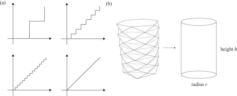
Figure 11: (a) the ‘Staircase paradox’. Fractal curves (for example the Koch curve) have similar non-convergence in metric- and curvature-related properties. (b) the ‘Schwarz Lantern’. In a cylinder of radius $r~{}(r>0)$ and height $h~{}(h>0)$ we inscribe a polyhedron as follows. Cut the cylinder into $m~{}(m\in\mathbb{Z}_{+})$ equal cylinders each of height $h/m$ by means of horizontal planes. Break each of the $m+1$ circles of intersection (including the upper and lower bases of the original cylinder) into $n~{}(n\in\mathbb{Z}_{+},~{}n\geq 2)$ equal parts so that the points of division on each circle lie beneath the midpoints of the points of division of the circle immediately above. We now take a pair of division points of each circle and the point lying directly above or below the midpoint of the pair of division points. These three points form a triangle, and the set of all such triangles forms a polyhedral surface inscribed in the original cylindrical surface. The area of each elementary triangle is $r\sin(\pi/n)\sqrt{h^{2}/m^{2}+r^{2}\left(1-\cos(\pi/n)\right)^{2}}=r\sin(\pi/n)\sqrt{h^{2}/m^{2}+4r^{2}\sin^{4}(\pi/2n)}$, and the total area is $2\left(n\sin(\pi/n)\right)rh\sqrt{1+4m^{2}r^{2}/h^{2}\sin^{4}(\pi/2n)}=2\pi rh\left(1+\pi^{4}m^{2}r^{2}/8h^{2}n^{4}\right)$, when $m,~{}n\rightarrow+\infty$. The area of the polyhedral surface depends on the limit of $m/n^{2}$, which can even reach infinity.

Theorem 1 indicates that, for each discrete net listed in Section F, once the initial value and parameter are bounded and converge to the initial condition for its smooth analogue listed in Section C, the discrete surface will converge to the corresponding smooth surface. Note that as explained in Section C and Section F, for each initial condition problem, the initial value and parameter are bounded, and the result – $x(u)$, $\partial x/\partial u_{1}$, $\partial x/\partial u_{2}$ are bounded and process a global Lipschitz constant.

In the Discussion section of the main text, we mentioned the convergence in distance does not guarantee the convergence of tangent plane, as well as other metric- and curvature- related properties. The zig-zag mode is a common reason for such non-convergence, akin to the Staircase paradox and the Schwarz Lantern illustrated in Figure 11.

Additionally, regarding the convergence of discrete conjugate net, Morvan and Thibert (2004) showed that convergence of the normal fields implies convergence of surface area. Hildebrandt et al. (2006) considerably generalized the result in Morvan and Thibert (2004): upon the convergence in distance, the convergence of metric tensor (the first fundamental form), surface area, normal vector field and mean curvature (the cotangent formula, Laplace-Beltrami operator) are equivalent. Once this convergence is met, it could be further inferred that arclength of coordinate curves/geodesics and Gaussian curvature will converge since they are dependent on the first fundamental form. Bauer et al. (2010) showed that discrete principal curvatures computed from a series of curvature line nets uniformly converge to the principal curvatures of the limit smooth surface. These results are not exhaustive, and there is still plenty of unexplored space.

Part II Quad-mesh rigid origami

Appendix H Flexibility of a quad-mesh rigid origami

The information of this section was previously provided in He et al. (2024) and He and Guest (2020). The idea of deriving the flexibility condition of a quad-mesh rigid origami is straightforward, which can be explained by ‘cutting’ through the paper to make the folding of each vertex independently driven (similar to single degree-of-freedom robotic arms), then consider the condition to properly ‘glue’ them together. We provide a graphical explanation of the original and the cut quad mesh in Figure 12(a) and (b), where we denote the tangent of half of folding angles by $y_{ij}$ and $w_{ij}~{}(i,~{}j\in\mathbb{Z}_{+})$ at the labelled creases.

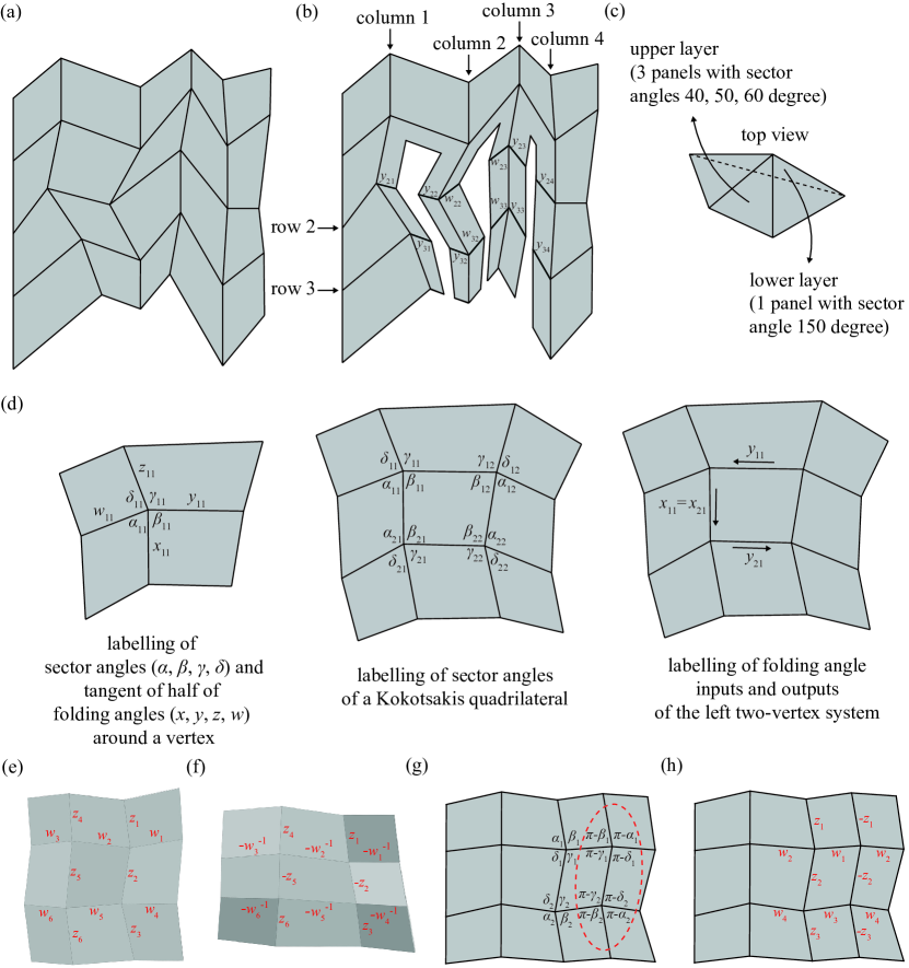
Figure 12: (a) and (b) explain how we ‘cut’ a quad-mesh rigid origami to make the interior of crease pattern a tree. When (b) is foldable, the motion of (b) agrees with a quad-mesh rigid origami if and only if all the folding angles $y$ and $w$ are identical as indicated in Eq. (44). (c) shows a vertex with sector angles $40^{\circ},~{}50^{\circ},~{}60^{\circ},~{}150^{\circ}$, which forms a double cover of a circular sector and hence remain rigid. (d) Labelling of a single-vertex, a Kokotsakis quadrilateral and a two-vertex system. (e) We use $\{z_{1},~{}z_{2},~{}z_{3},~{}z_{4},~{}z_{5},~{}z_{6}\}$ and $\{w_{1},~{}w_{2},~{}w_{3},~{}w_{4},~{}w_{5},~{}w_{6}\}$ to represent the tangent of half of the folding angles on these labelled interior creases. (f) the sector angles on panels of the middle row are replaced by their complements to $\pi$, other sector angles remain unchanged. (g) shows how a parallel strip is added, where the parallel strip is marked with a dashed cycle. In (h), the magnitude of new folding angles are labelled.

Proposition 5.

A quad-mesh rigid origami is flexible if and only if:

1. The cut quad-mesh is flexible. Consequently, there exists a smooth one-parameter flex for all $y_{ij}(t)$ and $w_{ij}(t)$ over $t\in[0,1]$.

2. for all $i,~{}j$,

   $$y_{i,j}(t)=y_{i,j+1}(t),~{}~{}w_{i,j}(t)=w_{i,j+1}(t),~{}~{}\mathrm{for~{}}t\in[0,1]$$ (44)

Note that condition [1] above is also essential since the cut quad-mesh might be rigid at special configurations. An example is provided in Figure 12(c). Further, Proposition 5 infers that:

Proposition 6.

(Schief et al., 2008) A quad-mesh rigid origami is flexible if and only if all its $3\times 3$ quad-mesh (Kokotsakis quadrilaterals) are flexible.

Izmestiev (2017) provided a nearly complete classification of flexible Kokotsakis quadrilaterals, which is the foundation of constructing large quad-mesh rigid origami. The terminology Kokotsakis quadrilateral is named after Antonios Kokotsakis, who studied the flexibility of these polyhedral surfaces in his PhD thesis in 1930s and described several flexible classes (Kokotsakis, 1933). At the same time, Sauer and Graf (1931) also found several classes. Recent works from Karpenkov (2010); Stachel (2010); Nawratil (2011, 2012) made solid contribution to this topic.

The library of flexible Kokotsakis quadrilaterals are derived in the complexified configuration space, where each Kokotsakis quadrilateral is flexible upon a system of constraints on the sector angles — most of these constraints are highly nonlinear. Our target is to explore all the ‘stitchings’ of Kokotsakis quadrilaterals that can form a quad-mesh rigid origami with the following requirements: 1) we require the construction of rigid origami to be ‘infinitely extendable’, in other words, not constrained in a finite grid. 2) we assume the number of variables is no less than the number of constraints; 3) for the admissible stitchings, we require the existence of valid real solutions from numerical examination; 4) on top of a valid numerical solution, we require the rigid origami to have an actual plotable folding motion. Otherwise, it might locate in the complexified configuration space and the structure will remain rigid even satisfying the flexibility constraint.

In terms of the flexibility condition of a Kokotsakis quadrilateral, it is convenient to consider the ‘compatibility’ of its two two-vertex systems, as shown in Figure 12(d). Here a Kokotsakis quadrilateral is ‘divided’ to its left and right two-vertex systems. For the left two-vertex system, we start from the input $y_{11}$, going through the left top vertex to obtain the output $x_{11}$. This output $x_{11}$ equals to the input of the left bottom vertex $x_{21}$, with which we can further calculate $y_{21}$. Consequently, the left two-vertex system generates its output $y_{21}$ as a function of its input $y_{11}$. Clearly, if and only if the $y_{21}$ calculated from the left and right two-vertex systems are identical for all $y_{11}$, the Kokotsakis quadrilateral will be flexible. A two-vertex system from $y_{11}$ to $y_{21}$ is clearly a compound function on the relation between adjacent folding angles of two degree-4 single-vertex rigid origami.

In He et al. (2023, Section 2), we present a comprehensive list of the various types of a single vertex. Notably, the terms (anti-)isogram, (anti-)deltoid, conic, and elliptic are included in this list.

We will now introduce two operations that can create a new flexible quad-mesh rigid origami from an existing one: these are called ’switching a strip’ and ’adding a parallel strip.’

Definition 4.

Switching a strip refers to replacing all the sector angles in a row or column of panels with their complements to $\pi$, while keeping the other sector angles unchanged. A visual representation of this operation can be seen in Figures 12(e) and 12(f). Adding a parallel strip means introducing an additional row or column of vertices with new interior creases, which are parallel to the creases of the adjacent row or column, as shown in Figures 12(g) and 12(h).

We will demonstrate that both operations — switching a strip and adding a parallel strip — preserve the flexibility of a quad-mesh rigid origami. Let’s first examine the case of switching a transverse strip. Consider switching the middle row of panels in Figure 12(e), where the sector angles are replaced by their complements to $\pi$ as shown in Figure 12(f).

The tangents of half the folding angles on the labelled interior creases are denoted by ${z_{1},~{}z_{2},~{}z_{3},~{}z_{4},~{}z_{5},~{}z_{6}}$ and ${w_{1},~{}w_{2},~{}w_{3},~{}w_{4},~{}w_{5},~{}w_{6}}$. After switching the strip, the folding angles change as follows:

$$\begin{gathered}\{z_{1},~{}z_{2},~{}z_{3},~{}z_{4},~{}z_{5},~{}z_{6}\}\rightarrow\{~{}z_{1},~{}-z_{2},~{}z_{3},~{}z_{4},~{}-z_{5},~{}z_{6}\}\\ \{w_{1},~{}w_{2},~{}w_{3},~{}w_{4},~{}w_{5},~{}w_{6}\}\rightarrow\{-w_{1}^{-1},~{}-w_{2}^{-1},~{}-w_{3}^{-1},~{}-w_{4}^{-1},~{}-w_{5}^{-1},~{}-w_{6}^{-1}\}\end{gathered}$$

Further details can be found in (He et al., 2023, Section 5). According to Proposition 5, switching a strip preserves the flexibility of a quad-mesh rigid origami. The proof for switching a longitudinal strip follows a similar reasoning. Next, after adding a parallel strip, the new folding angles are shown in Figure 12(h). As per Proposition 5, adding a parallel strip also maintains the flexibility of a quad-mesh rigid origami.

Appendix I V-hedra and V-surface

In this section we will give a comprehensive introduction to a V-hedron, as well as its smooth analogue called a V-surface. A V-hedron only contains proportional couplings of isograms, and is motion-guaranteed (He et al., 2024). The flexibility condition for a V-hedron is the compatible stitching of proportional couplings, or equivalently, the existence of a folded state. The properties of a V-hedron are listed below. The additional regularity condition for a V-hedron is at every vertex $\alpha\in(0,\pi),~{}\beta\in(0,\pi),~{}\alpha+\beta\neq\pi$, i.e, a V-hedron is not developable.

Proposition 7.

Features for a V-hedron:

1. An V-hedron has a flat-folded state where the folding angles around each vertex are $\{0,~{}\pi,~{}0,~{}\pi\}$, up to any cyclic permutation.

2. If a V-hedron has a non-flat rigidly folded state, this V-hedron is flexible.

3. Folding angles are constant along discrete coordinate curves.

4. (Sauer, 1970) The Gauss map of a V-hedron is a discrete Chebyshev net. A V-hedron is the only discrete conjugate net with a discrete Chebyshev Gauss map. See Figure 13(c).

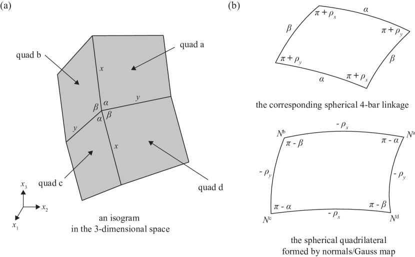
Figure 13: (a) A three-dimensional view of an isogram, where the surrounding quadrilaterals are labelled $\mathrm{a},~{}\mathrm{b},~{}\mathrm{c},~{}\mathrm{d}$. (b)The corresponding spherical 4-bar linkage of this isogram. (c) The spherical parallelogram formed by the Gauss map of surrounding panels.

We also say the Gauss map $N$ is a discrete spherical Chebyshev net since it is on the unit sphere. Clearly for any elementary quad of $N$, the opposite spherical arc lengths are also equal.

From the graphical explanation in Figure 15, a V-hedron is reciprocal-parallel related to a K-hedron (Sauer, 1950; Schief et al., 2008). This result is on top of the reciprocal-parallel relation between a discrete asymptotic net and a discrete conjugate net. Let $X(i)$ be a discrete asymptotic net, $Y(i)$ is another discrete surface such that $y(i_{1}+1,~{}i_{2})-y(i_{1},~{}i_{2})$ is parallel to $x(i_{1},~{}i_{2})-x(i_{1},~{}i_{2}-1)$; $y(i_{1}+1,~{}i_{2}+1)-y(i_{1},~{}i_{2}+1)$ is parallel to $x(i_{1},~{}i_{2}+1)-x(i_{1},~{}i_{2})$; $y(i_{1},~{}i_{2}+1)-y(i_{1},~{}i_{2})$ is parallel to $x(i_{1},~{}i_{2})-x(i_{1}-1,~{}i_{2})$; $y(i_{1}+1,~{}i_{2}+1)-y(i_{1}+1,~{}i_{2})$ is parallel to $x(i_{1}+1,~{}i_{2})-x(i_{1},~{}i_{2})$. From Figure 15, $X$ is ‘five points coplanar’ if and only if the elementary quadrilateral of $Y$ is planar.

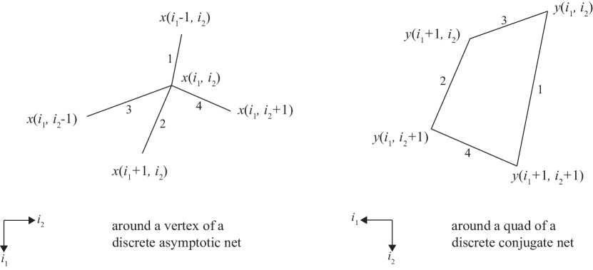
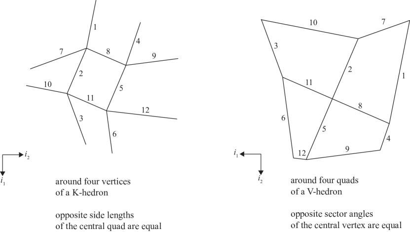
Figure 14: A figure illustrating the reciprocal-parallel relation between an asymptotic net and a conjugate net. Lines labelled with the same numbers are parallel.

Figure 15: A figure illustrating the reciprocal-parallel relation between a V-hedron and a K-hedron. Lines labelled with the same numbers are parallel.

Define the non-zero coefficients $a,b:\mathbb{Z}^{2}\rightarrow\mathbb{R},~{}a,~{}b\neq 0$, which live on the $i_{1}$ and $i_{2}$ grid lines, respectively:

$$\begin{gathered}y(i_{1}+1,~{}i_{2})-y(i_{1},~{}i_{2})=-b(i_{1},~{}i_{2})(x(i_{1},~{}i_{2})-x(i_{1},~{}i_{2}-1))\\ y(i_{1},~{}i_{2}+1)-y(i_{1},~{}i_{2})=a(i_{1},~{}i_{2})(x(i_{1},~{}i_{2})-x(i_{1}-1,~{}i_{2}))\end{gathered}$$

For simplicity we further require $ab>0$ over $\mathbb{Z}^{2}$, hence $X$ and $Y$ will share the same discrete normal vector field. Given a discrete asymptotic net $X$, $Y$ will be a discrete conjugate net determined upon $a,~{}b$ up to a translation. The inverse statement also holds. Given a discrete conjugate net $Y$, $X$ will be a discrete asymptotic net determined upon $a,~{}b$ up to a translation.

Next we will do a series of calculation to obtain the discrete Moutard equation, Eq. (40), for the normal vector field of a V-hedron. Let

$$\begin{gathered}a=\dfrac{x(i_{1},~{}i_{2})-x(i_{1}-1,~{}i_{2})}{\|x(i_{1},~{}i_{2})-x(i_{1}-1,~{}i_{2})\|},~{}~{}b=\dfrac{x(i_{1},~{}i_{2})-x(i_{1},~{}i_{2}-1)}{\|x(i_{1},~{}i_{2})-x(i_{1},~{}i_{2}-1)\|}\\ c=\dfrac{x(i_{1},~{}i_{2})-x(i_{1}+1,~{}i_{2})}{\|x(i_{1},~{}i_{2})-x(i_{1}+1,~{}i_{2})\|},~{}~{}d=\dfrac{x(i_{1},~{}i_{2})-x(i_{1},~{}i_{2}+1)}{\|x(i_{1},~{}i_{2})-x(i_{1},~{}i_{2}+1)\|}\end{gathered}$$

Note that $a,~{}b,~{}c,~{}d$ are temporary variables, which is updated from its previous usage. The Gauss map on each quadrilateral around vertex $i$ is

$$\begin{gathered}N^{\mathrm{a}}=\dfrac{d\times a}{\sin\alpha_{1}},~{}~{}N^{\mathrm{b}}=\dfrac{a\times b}{\sin\alpha_{2}}\\ N^{\mathrm{c}}=\dfrac{b\times c}{\sin\alpha_{1}},~{}~{}N^{\mathrm{d}}=\dfrac{c\times d}{\sin\alpha_{2}}\end{gathered}$$

since

$$\begin{gathered}N^{\mathrm{a}}\cdot N^{\mathrm{b}}=\cos\rho_{1},~{}~{}N^{\mathrm{b}}\cdot N^{\mathrm{c}}=\cos\rho_{2}\\ N^{\mathrm{c}}\cdot N^{\mathrm{d}}=\cos\rho_{1},~{}~{}N^{\mathrm{d}}\cdot N^{\mathrm{a}}=\cos\rho_{2}\end{gathered}$$

we have

$$\begin{gathered}(N^{\mathrm{a}}+N^{\mathrm{c}})\cdot(N^{\mathrm{b}}-N^{\mathrm{d}})=0\\ (N^{\mathrm{a}}-N^{\mathrm{c}})\cdot(N^{\mathrm{b}}+N^{\mathrm{d}})=0\\ \end{gathered}$$

Furthermore,

$$\begin{gathered}(N^{\mathrm{a}}+N^{\mathrm{c}})\cdot(N^{\mathrm{a}}-N^{\mathrm{c}})=0\\ (N^{\mathrm{b}}-N^{\mathrm{d}})\cdot(N^{\mathrm{b}}+N^{\mathrm{d}})=0\\ \end{gathered}$$

We could see that either $(N^{\mathrm{a}}+N^{\mathrm{c}})$ is parallel to $(N^{\mathrm{b}}+N^{\mathrm{d}})$, or $(N^{\mathrm{a}}-N^{\mathrm{c}})$ is parallel to $(N^{\mathrm{b}}-N^{\mathrm{d}})$. It can be verified from the derivation below:

$$\begin{gathered}N^{\mathrm{a}}+N^{\mathrm{c}}=\dfrac{d\times a+b\times c}{\sin\alpha_{1}}\\ N^{\mathrm{b}}+N^{\mathrm{d}}=\dfrac{a\times b+c\times d}{\sin\alpha_{2}}\\ (a\times b+c\times d)-(d\times a+b\times c)=(a+c)\times(b+d)=0\\ (a\times b+c\times d)+(d\times a+b\times c)=(a-c)\times(b-d)\end{gathered}$$

which makes use of the special geometry from the spherical quadrilateral Figure 13(c):

$$\begin{gathered}d-a=c-b\\ d-c=a-b\end{gathered}~{}~{}\Rightarrow~{}~{}a+c=b+d$$

It leads to the following relation on the normal vectors:

$$\triangle_{1}\triangle_{2}N =N^{\mathrm{b}}+N^{\mathrm{d}}-N^{\mathrm{a}}-N^{\mathrm{c}}$$

$$=\dfrac{\sin\alpha_{1}-\sin\alpha_{2}}{\sin\alpha_{1}+\sin\alpha_{2}}(N^{\mathrm{a}}+N^{\mathrm{b}}+N^{\mathrm{c}}+N^{\mathrm{d}})$$

$$=\left(\dfrac{\sin\alpha_{1}}{\sin\alpha_{2}}-1\right)(N^{\mathrm{a}}+N^{\mathrm{c}})$$

Assume there is no self-intersection, $N^{\mathrm{a}}-N^{\mathrm{c}}$ will not be parallel to $N^{\mathrm{b}}-N^{\mathrm{d}}$ (diagonals of a spherical parallelogram will not be parallel). From the symmetry of the Gauss map:

$$\begin{gathered}N^{\mathrm{a}}\cdot\dfrac{N^{\mathrm{a}}+N^{\mathrm{c}}}{||N^{\mathrm{a}}+N^{\mathrm{c}}||}=\dfrac{||N^{\mathrm{a}}+N^{\mathrm{c}}||}{2}\\ N^{\mathrm{b}}\cdot\dfrac{N^{\mathrm{a}}+N^{\mathrm{c}}}{||N^{\mathrm{a}}+N^{\mathrm{c}}||}=\dfrac{||N^{\mathrm{b}}+N^{\mathrm{d}}||}{2}\\ \end{gathered}$$

hence

$$\begin{gathered}N^{\mathrm{b}}+N^{\mathrm{d}}=\dfrac{N^{\mathrm{b}}\cdot(N^{\mathrm{a}}+N^{\mathrm{c}})}{N^{\mathrm{a}}\cdot(N^{\mathrm{a}}+N^{\mathrm{c}})}(N^{\mathrm{a}}+N^{\mathrm{c}})\\ \end{gathered}$$

which leads to the proposition below:

Proposition 8.

(Bobenko and Pinkall, 1996) Let $X:\mathbb{Z}^{2}\rightarrow\mathbb{R}^{3}$ be a V-hedron. The Gauss map $N$ is a discrete Moutard net satisfying the equation below:

$$\begin{gathered}\triangle_{1}\triangle_{2}N=\lambda(i_{1},~{}i_{2})\left(N(i_{1}+1,~{}i_{2})+N(i_{1},~{}i_{2}+1)\right)\\ \lambda(i_{1},~{}i_{2})=\dfrac{N(i_{1},~{}i_{2})\cdot\left(N(i_{1}+1,~{}i_{2})+N(i_{1},~{}i_{2}+1)\right)}{1+N(i_{1}+1,~{}i_{2})\cdot N(i_{1},~{}i_{2}+1)}-1\end{gathered}$$ (45)

Equivalently,

$$N(i_{1}+1,~{}i_{2}+1)=-N(i_{1},~{}i_{2})+(\lambda(i_{1},~{}i_{2})+1)\left(N(i_{1}+1,~{}i_{2})+N(i_{1},~{}i_{2}+1)\right)$$

The above proposition infers the following two constructions for a V-hedron. The first construction is based on the position of normal vectors on the coordinate curves. The second construction is based on the sector angles on the coordinate curves, hence the position of the rigid origami is determined up to an orthogonal transformation. The labelling is provided in Figure 6.

Initial Value 1

Two discrete coordinate curves $x(i_{2}=0)$ and $x(i_{1}=0)$ intersecting at $x(0,~{}0)$. $S^{\mathrm{a}}(-1,~{}0)=S^{\mathrm{c}}(0,~{}-1)$, $S^{\mathrm{b}}(-1,~{}-1)=S^{\mathrm{d}}(0,~{}0)$. Sector angles $S^{\mathrm{a}}(i_{1}\geq 0,~{}0)$; $S^{\mathrm{c}}(0,~{}i_{2}\geq 0)$; $S^{\mathrm{c}}(i_{1}\leq-1,~{}-1)$; $S^{\mathrm{a}}(-1,~{}i_{2}\leq-1)$.

Note that this input is equivalent to two boundary polylines and the direction vectors along them (Sauer, 1970).

Step 1a

From the above initial value we can immediately calculate $x(1,~{}1)$ and $N(0,~{}0)$, then from iterative calculation we could obtain $N(i_{1}\geq 1,~{}i_{2}=0)$ and $N(i_{1}=0,~{}i_{2}\geq 1)$.

Step 1b

Use Eq. (45) to calculate $N(i_{1}\geq 1,~{}i_{2}=1)$ and $N(i_{1}=1,~{}i_{2}\geq 1)$.

Step 1c

Use the equations below to locate $x(i_{1}\geq 2,~{}i_{2}=1)$ and $x(i_{1}=1,~{}i_{2}\geq 2)$:

$$\begin{dcases*}\triangle_{1}x(i_{1},~{}1)\mathrm{~{}is~{}parallel~{}to~{}}N(i_{1},~{}1)\times N(i,~{}0)\\ \triangle_{2}x(1,~{}i_{2})\mathrm{~{}is~{}parallel~{}to~{}}N(1,~{}i_{2})\times N(0,~{}j)\end{dcases*},~{}~{}i_{1},~{}i_{2}\in\mathbb{Z}_{+},~{}~{}i_{1},~{}i_{2}\geq 1$$

Step 1d

In the quadrant $\mathbb{Z}_{+}^{2}$, repeat Step 1b and Step 1c to obtain $x(i_{1}\geq 0,~{}i_{2}\geq 0)$ and its Gauss map $N(i_{1}\geq 0,~{}i_{2}\geq 0)$.

Step 1e

Use the same method as described in Step 1d to calculate the other three quadrants to obtain the entire mesh.

Regularity condition

Every step returns a non-degenerated and bounded result.

Note that Step 1b and Step 1c are equivalent to the condition requiring opposite sector angles equal. The intertwining calculation involving the Gauss map is relatively simple and does not require solving implicit equations.

Initial Value 2

Sector angles on the two discrete coordinate curves $S^{\mathrm{a}}(i_{1},~{}0)$; $S^{\mathrm{a}}(-1,~{}i_{2})$; $S^{\mathrm{b}}(i_{1},~{}-1)$; $S^{\mathrm{b}}(-1,~{}i_{2})$; $S^{\mathrm{c}}(i_{1},~{}-1)=S^{\mathrm{a}}(i_{1},~{}0)$; $S^{\mathrm{c}}(0,~{}i_{2})=S^{\mathrm{a}}(-1,~{}i_{2})$; $S^{\mathrm{d}}(i_{1},~{}0)=S^{\mathrm{b}}(i_{1},~{}-1)$; $S^{\mathrm{d}}(0,~{}i_{2})=S^{\mathrm{b}}(-1,~{}i_{2})$. Crease lengths on the two discrete coordinate curves $\|\triangle_{1}x(i_{1},~{}0)\|$ and $\|\triangle_{2}x(0,~{}i_{2})\|$.

Step 2a

From the above initial value, as the sum of sector angles on a quadrilateral equals to $2\pi$, and the opposite sector angles at each vertex are equal, we could calculate $S^{\mathrm{b}}(0,~{}0)$ and $S^{\mathrm{d}}(1,~{}1)$, then apply the equality of proportional dependence coefficients, we could calculate $S^{\mathrm{a}}(0,~{}1)$ and $S^{\mathrm{c}}(1,~{}0)$. Next, from iterative calculation we will obtain the sector angles on $x(i_{2}=1)$ and $x(i_{1}=1)$.

Step 2b

In the quadrant $\mathbb{Z}_{+}^{2}$, repeat Step 2a to obtain the sector angles of $x(i_{1}\geq 0,~{}i_{2}\geq 0)$.

Step 2c

Use the same method described in Step 2b to calculate the other three quadrants to obtain the sector angles of the entire mesh.

Step 2d

After all the sector angles are determined, the crease lengths on the two discrete coordinate curves will fully determine the shape of the quad-mesh, up to an orthogonal transformation.

Regularity condition

The result of calculating a sector angle always falls in $(0,\pi)$.

Next we explain the smooth analogue of a V-hedron – called a V-surface. A V-hedron is a discrete geodesic conjugate net. From Section E, the smooth analogue of a V-hedron should be a smooth geodesic conjugate net. The additional regularity condition for a V-surface is non-developable, which means not being an orthogonal net simultaneously. From Eq. (26), the condition for a surface parametrization to form a geodesic conjugate net, i.e, to be a V-surface is:

$$\begin{gathered}\begin{dcases}\dfrac{\partial^{2}x}{\partial u_{1}^{2}}\mathrm{~{}is~{}on~{}the~{}plane~{}spanned~{}from~{}}N\mathrm{~{}and~{}}\dfrac{\partial x}{\partial u_{1}}\\ \dfrac{\partial^{2}x}{\partial u_{2}^{2}}\mathrm{~{}is~{}on~{}the~{}plane~{}spanned~{}from~{}}N\mathrm{~{}and~{}}\dfrac{\partial x}{\partial u_{2}}\end{dcases}~{}~{}\Leftrightarrow~{}~{}\begin{dcases}2\mathrm{I}_{11}\dfrac{\partial\mathrm{I}_{12}}{\partial u_{1}}=\mathrm{I}_{11}\dfrac{\partial\mathrm{I}_{11}}{\partial u_{2}}+\mathrm{I}_{12}\dfrac{\partial\mathrm{I}_{11}}{\partial u_{1}}\\ 2\mathrm{I}_{22}\dfrac{\partial\mathrm{I}_{12}}{\partial u_{2}}=\mathrm{I}_{22}\dfrac{\partial\mathrm{I}_{22}}{\partial u_{1}}+\mathrm{I}_{12}\dfrac{\partial\mathrm{I}_{22}}{\partial u_{2}}\\ \end{dcases}\\ \mathrm{II}_{12}=0\end{gathered}$$

Recall that the principal curvatures are from the simultaneous diagonalization of the first and second fundamental forms. There exists a $2\times 2$ matrix $A$ such that:

$$\begin{gathered}\begin{bmatrix}\mathrm{I}_{11}&\mathrm{I}_{12}\\ \mathrm{I}_{12}&\mathrm{I}_{22}\end{bmatrix}=AA^{\mathrm{T}}\\ \begin{bmatrix}\mathrm{II}_{11}&\mathrm{II}_{12}\\ \mathrm{II}_{12}&\mathrm{II}_{22}\end{bmatrix}=A\begin{bmatrix}\kappa_{1}&0\\ 0&\kappa_{2}\end{bmatrix}A^{\mathrm{T}}\end{gathered}$$

We could infer that a sphere is not a V-surface. If so, from the above relation $\mathrm{I}_{12}=\mathrm{II}_{12}=0$, hence on top of being a geodesic conjugate net, the surface is also an orthogonal Chebyshev net, which has zero Gaussian curvature.

A V-surface has geometric properties parallel to Proposition 7.

Proposition 9.

Features for a V-surface:

1. (Bianchi, 1890) A V-surface admits a one-parameter flex (isometric deformation) and preserves to be a V-surface in this flex.

2. The Gauss map of a V-surface is a Chebyshev net. A V-surface is the only conjugate net with a Chebyshev Gauss map.

In particular we will prove [1] from calculation. The Gauss-Mainardi-Codazzi Equations yield:

$$\begin{dcases}\dfrac{\partial\Gamma^{2}_{12}}{\partial u_{1}}+\Gamma^{2}_{12}\Gamma^{2}_{12}-\Gamma^{1}_{11}\Gamma^{2}_{12}=-\mathrm{I}_{11}\kappa_{\mathrm{G}}\\ \dfrac{\partial\mathrm{II}_{11}}{\partial u_{2}}=\mathrm{II}_{11}\Gamma^{1}_{12}\\ \dfrac{\partial\mathrm{II}_{22}}{\partial u_{1}}=\mathrm{II}_{22}\Gamma^{2}_{12}\\ \end{dcases}$$

The flex parametrized by $t\in I$ where the first fundamental form $\mathrm{I}$ is preserved and

$$\begin{gathered}\mathrm{II}_{11}(t)=\lambda(t)\mathrm{II}_{11}(0)\\ \mathrm{II}_{12}(t)=0\\ \mathrm{II}_{22}(t)=\dfrac{1}{\lambda(t)}\mathrm{II}_{22}(0)\\ \end{gathered},~{}~{}\lambda:I\rightarrow\mathbb{R}$$ (46)

meets the Gauss-Mainardi-Codazzi Equations. A V-surface is the only conjugate net that has such a flex.

A V-surface is reciprocal-parallel related to a K-surface (asymptotic Chebyshev net, Section B). This result is on top of the reciprocal-parallel relation between an asymptotic net and a conjugate net. A conjugate net is reciprocal-parallel related with an asymptotic net. Let $X(u)$ be an asymptotic net, $Y(u)$ is another surface such that $\partial y/\partial u_{1}$ is parallel to $\partial x/\partial u_{2}$ and $\partial y/\partial u_{2}$ is parallel to $\partial x/\partial u_{1}$.

$$\begin{gathered}\dfrac{\partial y}{\partial u_{1}}=-b\dfrac{\partial x}{\partial u_{2}},~{}~{}\dfrac{\partial y}{\partial u_{2}}=a\dfrac{\partial x}{\partial u_{1}}\\ a,~{}b:I^{2}\rightarrow\mathbb{R}\mathrm{~{}are~{}smooth~{}functions},~{}a,~{}b\neq 0\end{gathered}$$

For simplicity we further require $ab>0$ over $I^{2}$, hence $X$ and $Y$ will share the same normal vector field:

$$N^{y}=\dfrac{\dfrac{\partial y}{\partial u_{1}}\times\dfrac{\partial y}{\partial u_{2}}}{\left\|\dfrac{\partial y}{\partial u_{1}}\times\dfrac{\partial y}{\partial u_{2}}\right\|}=\dfrac{\dfrac{\partial x}{\partial u_{1}}\times\dfrac{\partial x}{\partial u_{2}}}{\left\|\dfrac{\partial x}{\partial u_{1}}\times\dfrac{\partial x}{\partial u_{2}}\right\|}=N^{x}$$

$$\begin{dcases}\mathrm{II}_{11}^{x}=0\\ \mathrm{II}_{22}^{x}=0\\ \end{dcases}~{}~{}\Leftrightarrow~{}~{}\mathrm{II}_{12}^{y}=0$$

The coefficients should satisfy the compatibility condition from $\partial(\partial y/\partial u_{1})/\partial u_{2}=\partial(\partial y/\partial u_{2})/\partial u_{1}$, using the Christoffel symbols, Eq. (4):

$$\begin{gathered}\dfrac{\partial b}{\partial u_{2}}+a\Gamma_{11}^{2x}+b\Gamma_{22}^{2x}=0\\ \dfrac{\partial a}{\partial u_{1}}+a\Gamma_{11}^{1x}+b\Gamma_{22}^{1x}=0\\ \end{gathered}$$ (47)

The compatibility condition is a first-order hyperbolic system for $a,~{}b$, which is well-posed (Section C), hence $a,~{}b$ are determined upon the initial value on the stationary directions $a(u_{1},~{}0)$ and $b(0,~{}u_{2})$. Given an asymptotic net $X$, $Y$ will be a conjugate net determined upon $a,~{}b$ up to a translation. The inverse statement also holds. Given a conjugate net $Y$, $X$ will be an asymptotic net determined upon $a,~{}b$ up to a translation.

Now on top of being asymptotic, assume $X$ is a Chebyshev net:

$$\begin{dcases}\dfrac{\partial^{2}x}{\partial u_{1}\partial u_{2}}\cdot\dfrac{\partial x}{\partial u_{1}}=0\\ \dfrac{\partial^{2}x}{\partial u_{1}\partial u_{2}}\cdot\dfrac{\partial x}{\partial u_{2}}=0\\ \end{dcases}~{}~{}\Leftrightarrow~{}~{}\begin{dcases}\dfrac{\partial}{\partial u_{1}}\left(\dfrac{1}{b}\dfrac{\partial y}{\partial u_{1}}\right)\cdot\dfrac{\partial y}{\partial u_{2}}=0\\ \dfrac{\partial}{\partial u_{1}}\left(\dfrac{1}{b}\dfrac{\partial y}{\partial u_{1}}\right)\cdot\dfrac{\partial y}{\partial u_{1}}=0\\ \dfrac{\partial}{\partial u_{2}}\left(\dfrac{1}{a}\dfrac{\partial y}{\partial u_{2}}\right)\cdot\dfrac{\partial y}{\partial u_{2}}=0\\ \dfrac{\partial}{\partial u_{2}}\left(\dfrac{1}{a}\dfrac{\partial y}{\partial u_{2}}\right)\cdot\dfrac{\partial y}{\partial u_{1}}=0\\ \end{dcases}$$

which shows that

$$\begin{gathered}\begin{dcases}\dfrac{\partial}{\partial u_{1}}\left(\dfrac{1}{b}\right)\mathrm{I}_{12}^{y}+\dfrac{1}{b}\dfrac{\partial^{2}y}{\partial u_{1}^{2}}\cdot\dfrac{\partial y}{\partial u_{2}}=0\\ \dfrac{\partial}{\partial u_{1}}\left(\dfrac{1}{b}\right)\mathrm{I}_{11}^{y}+\dfrac{1}{b}\dfrac{\partial^{2}y}{\partial u_{1}^{2}}\cdot\dfrac{\partial y}{\partial u_{1}}=0\\ \dfrac{\partial}{\partial u_{1}}\left(\dfrac{1}{a}\right)\mathrm{I}_{22}^{y}+\dfrac{1}{a}\dfrac{\partial^{2}y}{\partial u_{2}^{2}}\cdot\dfrac{\partial y}{\partial u_{2}}=0\\ \dfrac{\partial}{\partial u_{1}}\left(\dfrac{1}{a}\right)\mathrm{I}_{12}^{y}+\dfrac{1}{a}\dfrac{\partial^{2}y}{\partial u_{2}^{2}}\cdot\dfrac{\partial y}{\partial u_{1}}=0\\ \end{dcases}~{}~{}\Rightarrow~{}~{}\begin{dcases}\dfrac{\dfrac{\partial^{2}y}{\partial u_{1}^{2}}\cdot\dfrac{\partial y}{\partial u_{1}}}{\dfrac{\partial^{2}y}{\partial u_{1}^{2}}\cdot\dfrac{\partial y}{\partial u_{2}}}=\dfrac{\mathrm{I}_{11}^{y}}{\mathrm{I}_{12}^{y}}\\ \dfrac{\dfrac{\partial^{2}y}{\partial u_{2}^{2}}\cdot\dfrac{\partial y}{\partial u_{2}}}{\dfrac{\partial^{2}y}{\partial u_{2}^{2}}\cdot\dfrac{\partial y}{\partial u_{1}}}=\dfrac{\mathrm{I}_{22}^{y}}{\mathrm{I}_{12}^{y}}\\ \end{dcases}\end{gathered}$$

Geometrically it means that in the non-orthogonal frame $(\partial y/\partial u_{1},~{}\partial y/\partial u_{2},~{}N)$, $\partial^{2}y/\partial u_{1}^{2}$ has no component along $\partial y/\partial u_{1}$, and $\partial^{2}y/\partial u_{2}^{2}$ has no component along $\partial y/\partial u_{2}$, hence $Y$ is a geodesic net.

Example 1.

(Izmestiev et al., 2024a) Consider a K-surface:

$$x(u_{1},~{}u_{2})=\begin{bmatrix}\cos(u_{1}-u_{2})/\cosh(u_{1}+u_{2})\\ \sin(u_{1}-u_{2})/\cosh(u_{1}+u_{2})\\ u_{1}+u_{2}-\tanh(u_{1}+u_{2})\end{bmatrix}$$

The second fundamental form is:

$$\begin{bmatrix}\mathrm{II}_{11}^{x}&\mathrm{II}_{12}^{x}\\ \mathrm{II}_{12}^{x}&\mathrm{II}_{22}^{x}\end{bmatrix}=\begin{bmatrix}0&-\dfrac{2\tanh(u_{1}+u_{2})}{\cosh(u_{1}+u_{2})}\\[10.0pt] -\dfrac{2\tanh(u_{1}+u_{2})}{\cosh(u_{1}+u_{2})}&0\end{bmatrix}$$

The compatibility condition Eq. (47) has a solution $a=b$:

$$\dfrac{\partial a}{\partial u_{1}}=\dfrac{\partial a}{\partial u_{2}}=-\dfrac{2a}{\cosh(u_{1}+u_{2})\sinh(u_{1}+u_{2})}$$

and hence:

$$a=b=\mathrm{Const}\cdot\left(\dfrac{1+\exp(2(u_{1}+u_{2}))}{1-\exp(2(u_{1}+u_{2}))}\right)^{2}$$

The V-surface is now ready to be obtain by integration. For example if $\mathrm{Const}=1$, under a suitable sign choice:

$$y(u_{1},~{}u_{2})=\begin{bmatrix}\dfrac{2(\cosh(u_{1}+u_{2})+\sinh(u_{1}+u_{2}))\cos(u_{1}-u_{2})}{\cosh(2u_{1}+2u_{2})+\sinh(2u_{1}+2u_{2})+1}\\[10.0pt] \dfrac{2(\cosh(u_{1}+u_{2})+\sinh(u_{1}+u_{2}))\sin(u_{1}-u_{2})}{\cosh(2u_{1}+2u_{2})+\sinh(2u_{1}+2u_{2})+1}\\ u_{1}-u_{2}\end{bmatrix}$$

We could see that the V-surface is in the form of $(\rho\cos\theta,~{}\rho\sin\theta,~{}\theta)$, hence is actually a helicoid. Concurrently, we can construct a V-hedron in the shape of a helicoid from a K-hedron in the shape of a pseudosphere using grid values of $a,~{}b$ calculated above.

Appendix J T-hedra and T-surface

In this section we will focus on the details of a T-hedron, as well as its smooth analogue called a T-surface. The information here is an excerpt from Izmestiev et al. (2024b). A T-hedron only contains involutive couplings of orthodiagonal vertices, and is also motion-guaranteed (He et al., 2024). To be specific, consider the grid depicted in Figure 16 as an example, the condition of being orthodiagonal vertices is:

$$\begin{gathered}\cos\alpha_{11}\cos\gamma_{11}=\cos\beta_{11}\cos\delta_{11},~{}~{}\cos\alpha_{12}\cos\gamma_{12}=\cos\beta_{12}\cos\delta_{12}\\ \cos\alpha_{21}\cos\gamma_{21}=\cos\beta_{21}\cos\delta_{21},~{}~{}\cos\alpha_{22}\cos\gamma_{22}=\cos\beta_{22}\cos\delta_{22}\\ \end{gathered}$$

The condition of the involution factor being equal for all the four pairs in a Kokotsakis quadrilateral is:

$$\begin{gathered}\dfrac{\tan\alpha_{11}}{\tan\beta_{11}}=\dfrac{\tan\alpha_{21}}{\tan\beta_{21}},~{}~{}\dfrac{\tan\alpha_{12}}{\tan\beta_{12}}=\dfrac{\tan\alpha_{22}}{\tan\beta_{22}}\\ \dfrac{\tan\gamma_{11}}{\tan\beta_{11}}=\dfrac{\tan\gamma_{21}}{\tan\beta_{21}},~{}~{}\dfrac{\tan\gamma_{12}}{\tan\beta_{12}}=\dfrac{\tan\gamma_{22}}{\tan\beta_{22}}\end{gathered}$$

The condition of the amplitude being equal is:

$$\dfrac{\cos\beta_{11}}{\cos\beta_{21}}=\dfrac{\cos\beta_{12}}{\cos\beta_{22}}$$

As $\beta_{11}+\beta_{21}+\beta_{12}+\beta_{22}=2\pi$, we could see that either $\beta_{11}+\beta_{21}=\beta_{12}+\beta_{22}=\pi$ or $\beta_{11}+\beta_{12}=\beta_{21}+\beta_{22}=\pi$, i.e., every elementary quadrilateral is a trapezoid. Further, if $\beta_{11}+\beta_{21}=\beta_{12}+\beta_{22}=\pi$, the nearby Kokotsakis quadrilaterals must have $\beta_{21}+\beta_{31}=\beta_{22}+\beta_{32}=\pi$ and $\beta_{12}+\beta_{22}=\beta_{13}+\beta_{23}=\pi$, etc. In combination with each vertex being orthodiagonal and every pair of vertices forms an involutive coupling, we list the properties of a T-hedron below, which is also visualized in Figure 16.

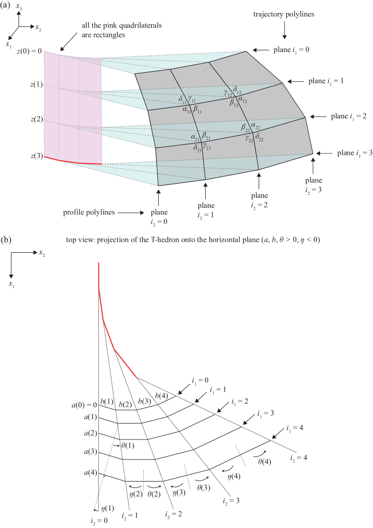
Figure 16: (a) shows a T-hedron (coloured grey) and its associated geometry. The sector angles are labelled $\alpha_{i_{1},~{}i_{2}},~{}\beta_{i_{1},~{}i_{2}},~{}\gamma_{i_{1},~{}i_{2}},~{}\delta_{i_{1},~{}i_{2}},~{}i_{1},~{}i_{2}\in\mathbb{Z}$. The horizontal planes ($i_{1}=j,~{}j\in\mathbb{Z}$) are coloured green, and all the intersections of the horizontal planes and the longitudinal ($i_{2}=k,~{}k\in\mathbb{Z}$) planes are drawn with dashed lines. These dashed lines intersect with each other consecutively, forming rectangles (coloured pink). (b) is a top view of the projection of a T-hedron to the horizontal plane, which also graphically explains coordinates $a(i_{1})$, signed crease lengths $b(i_{2})$, signed angles $\eta(i_{2})$, $\theta(i_{2})$.

Proposition 10.

Features for a T-hedron:

1. Every elementary quadrilateral is a trapezoid, the parallel sides of all the trapezoids are all horizontal or all longitudinal.

2. Every row of vertices ($i_{1}=j,~{}j\in\mathbb{Z}$) is coplanar. Every column of vertices ($i_{2}=k,~{}k\in\mathbb{Z}$) is coplanar.

3. Plane $i_{1}=j,~{}j\in\mathbb{Z}$ is orthogonal to plane $i_{2}=k,~{}k\in\mathbb{Z}$.

4. Either all the horizontal planes $i_{1}=j,~{}j\in\mathbb{Z}$ are parallel to each other (Figure 16), or all the longitudinal planes are parallel to each other.

Statement [4] holds since if not all horizontal planes are parallel to each other, we could take two intersecting horizontal planes, all the longitudinal planes will be perpendicular to this intersection, hence all the longitudinal planes are parallel to each other.

To reach an analytical description of a T-hedron, we will use the quantities graphically defined in Figure 16(b) to write the coordinate of every vertex of the T-hedron: $\eta(1)\in(-\pi/2,\pi/2)$ is the rotation from the projection of plane $i_{2}=0$ to the line perpendicular to the parallel edges of trapezoid on column 0; $\theta(1)\in(-\pi/2,\pi/2)$ is the rotation from the aforementioned line to the projection of plane $i_{2}=1$, $\eta(i_{2})\in(-\pi/2,\pi/2)$ and $\theta(i_{2})\in(-\pi/2,\pi/2)$ are defined in a similar way. $a(i_{1})\in\mathbb{R}$ are the coordinates along the $x_{1}$ axis of the projection of row $i_{1}$, column $0$ of the T-hedron; $b(i_{2})\in\mathbb{R}$ are the signed crease lengths of the projection of row $0$, column $i_{2}$ of the T-hedron. In Figure 16 all the $a(i_{1}\neq 0)$, $b(i_{2})$ are positive. The projection of each row $i_{1}=j$ of the T-hedron is called a trajectory polyline. The projection of each column $i_{2}=k$ of the T-hedron is called a profile polyline. In addition to being a discrete surface, we further apply the regularity condition to the data mentioned above:

Additional regularity condition

$b(i_{2})\neq 0$ for all $i_{2}$, $z(0)\neq z(1)\neq\cdots\neq z(i_{1})$ for all $i_{1}$.

Let

$$\phi(i_{2})=\sum\limits_{k=1}^{i_{2}}\eta(k)+\sum\limits_{k=1}^{i_{2}}\theta(k),~{}~{}\psi(i_{2})=\sum\limits_{k=1}^{i_{2}}\eta(k)+\sum\limits_{k=1}^{i_{2}-1}\theta(k)$$

The vertices on row $i_{1}$ are on the same horizontal plane:

$$x(i_{1},~{}i_{2})=\begin{bmatrix}x_{1}(i_{1},~{}i_{2})\\ x_{2}(i_{1},~{}i_{2})\\ z(i_{1})\end{bmatrix}$$ (48)

the coordinates of vertices on the first row $i_{1}=0$ is:

$$\begin{bmatrix}x_{1}(0,~{}i_{2})\\ x_{2}(0,~{}i_{2})\end{bmatrix}=\sum\limits_{k=1}^{i_{2}}b(k)\begin{bmatrix}-\sin\psi(k)\\ \cos\psi(k)\end{bmatrix}$$

The signed distance between $[x_{1}(i_{1},~{}1);~{}x_{2}(i_{1},~{}1)]$ and $[x_{1}(i_{1},~{}0);~{}x_{2}(i_{1},~{}0)]$ on the horizontal plane is:

$$a(i_{1})\dfrac{\cos\eta(1)}{\cos\theta(1)}$$

Similarly, the signed distance between $[x_{1}(i_{1},~{}i_{2});~{}x_{2}(i_{1},~{}i_{2})]$ and $[x_{1}(i_{1},~{}0);~{}x_{2}(i_{1},~{}0)]$ on the horizontal plane is:

$$\begin{gathered}a(i_{1})\dfrac{\cos\eta(1)\cos\eta(2)\cdots\cos\eta(i_{2})}{\cos\theta(1)\cos\theta(2)\cdots\cos\theta(i_{2})}=a(i_{1})\prod\limits_{k=1}^{i_{2}}\dfrac{\cos\eta(k)}{\cos\theta(k)}=a(i_{1})c(i_{2})\\ \mathrm{~{}if~{}set~{}}c(i_{2})=\prod\limits_{k=1}^{i_{2}}\dfrac{\cos\eta(k)}{\cos\theta(k)}\end{gathered}$$

then we could calculate the coordinate on each column:

$$\begin{bmatrix}x_{1}(i_{1},~{}i_{2})\\ x_{2}(i_{1},~{}i_{2})\end{bmatrix} =\begin{bmatrix}x_{1}(0,~{}i_{2})\\ x_{2}(0,~{}i_{2})\end{bmatrix}+a(i_{1})c(i_{2})\begin{bmatrix}\cos\phi(i_{2})\\ \sin\phi(i_{2})\end{bmatrix}$$ (49)

$$=\sum\limits_{k=1}^{i_{2}}b(k)\begin{bmatrix}-\sin\psi(k)\\ \cos\psi(k)\end{bmatrix}+a(i_{1})c(i_{2})\begin{bmatrix}\cos\phi(i_{2})\\ \sin\phi(i_{2})\end{bmatrix}$$

To summarize, the dataset $\eta(i_{2}),~{}\theta(i_{2}),~{}a(i_{1}),~{}b(i_{2}),~{}z(i_{1})$, or equivalently $\phi(i_{2}),~{}\psi(i_{2}),~{}a(i_{1}),~{}b(i_{2}),~{}z(i_{1})$ uniquely determines a T-hedron upon the regularity condition.

Izmestiev et al. (2024b) also provides several special T-hedra with graphical illustration, including 1) the molding surface: $\eta(i_{2})=\theta(i_{2})$. Here every trapezoid is isosceles, consequently, every trapezoid have same sector angles; 2) the axial surface: the trajectory polyline at $i_{1}=0$ degenerates to a single point; 3) surface of revolution: being both a molding surface and an axial surface; 4) translational surface: the trajectory polyline at $i_{1}=0$ degenerates to a single point at infinity. Here every trapezoid is a parallelogram.

Next we will calculate the coordinates of all the vertices $x(i;~{}t),~{}t\in[-\epsilon,\epsilon],~{}\epsilon\in(0,1)$ in its one-parameter folding motion. By applying a proper rotation and translation, all the green planes of $x(i;~{}t)$ in Figure 16(a) could be set horizontal, with $z(0;~{}t)=0$ for all $t\in[-\epsilon,\epsilon]$. The deformed T-hedron has the parametrization below:

$$x(i_{1},~{}i_{2};~{}t)=\begin{bmatrix}x_{1}(i_{1},~{}i_{2};~{}t)\\ x_{2}(i_{1},~{}i_{2};~{}t)\\ z(i_{1};~{}t)\end{bmatrix}$$

$$\begin{bmatrix}x_{1}(i_{1},~{}i_{2};~{}t)\\ x_{2}(i_{1},~{}i_{2};~{}t)\end{bmatrix}=\sum\limits_{k=1}^{i_{2}}b(k)\begin{bmatrix}-\sin\psi(k;~{}t)\\ \cos\psi(k;~{}t)\end{bmatrix}+a(i_{1};~{}t)c(i_{2};~{}t)\begin{bmatrix}\cos\phi(i_{2};~{}t)\\ \sin\phi(i_{2};~{}t)\end{bmatrix}$$

$$\phi(i_{2};~{}t)=\sum\limits_{k=1}^{i_{2}}\eta(k;~{}t)+\sum\limits_{k=1}^{i_{2}}\theta(k;~{}t),~{}~{}\psi(i_{2};~{}t)=\sum\limits_{k=1}^{i_{2}}\eta(k;~{}t)+\sum\limits_{k=1}^{i_{2}-1}\theta(k;~{}t)$$

Note that $b(i_{2})$ is irrelevant of $k$. We will see it from the analysis below.

We will analyse how a T-hedron deforms from its projection on the horizontal planes. In Figure 17(b) we extract four trapezoids $(i_{1},~{}i_{2})=(0,~{}0)$, $(0,~{}1)$, $(1,~{}0)$, $(1,~{}1)$ (coloured black) from Figure 16 and consider its deformed state (coloured red). Take quadrilateral $ABED$ as example, the key geometrical constraint is $DD^{\prime}E^{\prime}E$ preserves to be a rectangle. Further, $BCFE$ will deform to $BCF^{\prime}E^{\prime}$ under this constraint: $EE^{\prime}F^{\prime}F$ preserves to be a rectangle after a possible rotation and translation of $BCF^{\prime}E^{\prime}$. Here, $BCHG$ is rotated from $BCF^{\prime}E^{\prime}$, and $EFHG$ preserves to be a rectangle. From how the deformed state is generated, we could see that, $b(i_{2})$ preserves in the motion for all $i_{2}$. Now consider the first row of quadrilaterals, we could list $i_{2}+1$ equations from the crease lengths of the T-hedron being preserved for all $t\in[-\epsilon,\epsilon]$. Note that $a(0;~{}t)=0$ for all $t\in[-\epsilon,\epsilon]$, but we still write it for consistency with the other rows of quadrilaterals.

$$\begin{dcases}\begin{split}&\quad(a(1;~{}0)-a(0;~{}0))^{2}+(z(1;~{}0)-z(0;~{}0))^{2}\\ &=(a(1;~{}t)-a(0;~{}t))^{2}+(z(1;~{}t)-z(0;~{}t))^{2}\end{split}\\ \begin{split}&\quad(a(1;~{}0)-a(0;~{}0))^{2}c^{2}(1;~{}0)+(z(1;~{}0)-z(0;~{}0))^{2}\\ &=(a(1;~{}t)-a(0;~{}t))^{2}c^{2}(1;~{}t)+(z(1;~{}t)-z(0;~{}t))^{2}\end{split}\\ \cdots\\ \begin{split}&\quad(a(1;~{}0)-a(0;~{}0))^{2}c^{2}(i_{2};~{}0)+(z(1;~{}0)-z(0;~{}0))^{2}\\ &=(a(1;~{}t)-a(0;~{}t))^{2}c^{2}(i_{2};~{}t)+(z(1;~{}t)-z(0;~{}t))^{2}\end{split}\end{dcases}$$

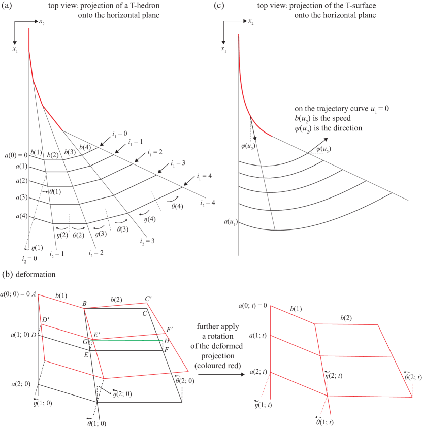
Figure 17: An illustration to the deformation of a T-hedron from its projection onto the horizontal plane. We let the horizontal plane remain horizontal and the vertex $x(0,~{}0)$ fixed – consequently $a(0;~{}t)=0$ for all $t$. (b) shows how the trapezoid projection deforms from (a). (c) depicts the projection of the corresponding T-surface onto the horizontal plane.

From these equations, we could draw a parametrization starting with:

$$a(1;~{}t)=a(1;~{}0)\sqrt{1+t}$$ (50)

Consequently,

$$c^{2}(i_{2};~{}t)=\dfrac{c^{2}(i_{2};~{}0)+t}{1+t},~{}~{}\mathrm{for~{}all~{}}i_{2}$$ (51)

Further from Figure 17(b):

$$\begin{gathered}a(1;~{}0)c(i_{2}-1;~{}0)\sin\eta(i_{2};~{}0)=a(1;~{}t)c(i_{2}-1;~{}t)\sin\eta(i_{2};~{}t)\\ a(1;~{}0)c(i_{2};~{}0)\sin\theta(i_{2};~{}0)=a(1;~{}t)c(i_{2};~{}t)\sin\theta(i_{2};~{}t)\end{gathered}$$

that is to say

$$\begin{gathered}\dfrac{\sin\eta(i_{2};~{}t)}{\sin\eta(i_{2};~{}0)}=\dfrac{a(1;~{}0)c(i_{2}-1;~{}0)}{a(1;~{}t)c(i_{2}-1;~{}t)}=\dfrac{c(i_{2}-1;~{}0)}{\sqrt{c^{2}(i_{2}-1;~{}0)+t}}\\ \dfrac{\sin\theta(i_{2};~{}t)}{\sin\theta(i_{2};~{}0)}=\dfrac{a(1;~{}0)c(i_{2};~{}0)}{a(1;~{}t)c(i_{2};~{}t)}=\dfrac{c(i_{2};~{}0)}{\sqrt{c^{2}(i_{2};~{}0)+t}}\\ \end{gathered}$$

Next we will calculate $z(i_{1};~{}t)$, from the second row of quadrilateral:

$$\begin{dcases}\begin{split}&\quad(a(i_{1};~{}0)-a(i_{1}-1;~{}0))^{2}+(z(i_{1};~{}0)-z(i_{1}-1;~{}0))^{2}\\ &=(a(i_{1};~{}t)-a(i_{1}-1;~{}t))^{2}+(z(i_{1};~{}t)-z(i_{1}-1;~{}t))^{2}\end{split}\\ \begin{split}&\quad(a(i_{1};~{}0)-a(i_{1}-1;~{}0))^{2}c^{2}(1;~{}0)+(z(i_{1};~{}0)-z(i_{1}-1;~{}0))^{2}\\ &=(a(i_{1};~{}t)-a(i_{1}-1;~{}t))^{2}c^{2}(1;~{}t)+(z(i_{1};~{}t)-z(i_{1}-1;~{}t))^{2}\\ \end{split}\\ \cdots\\ \begin{split}&\quad(a(i_{1};~{}0)-a(i_{1}-1;~{}0))^{2}c^{2}(i_{2};~{}0)+(z(i_{1};~{}0)-z(i_{1}-1;~{}0))^{2}\\ &=(a(i_{1};~{}t)-a(i_{1}-1;~{}t))^{2}c^{2}(i_{2};~{}t)+(z(i_{1};~{}t)-z(i_{1}-1;~{}t))^{2}\end{split}\end{dcases}$$

The result is an iterative expression for $z(i_{1};~{}t)$:

$$a(i_{1};~{}t)=a(i_{1};~{}0)\sqrt{1+t}\mathrm{~{}~{}for~{}all~{}}i_{1}$$ (52)

$$\begin{gathered}z^{2}(1;~{}t)=z^{2}(1;~{}0)-t(a(1;~{}0)-a(0;~{}0))^{2}\\ (z(2;~{}t)-z(1;~{}t))^{2}=(z(2;~{}0)-z(1;~{}0))^{2}-t(a(2;~{}0)-a(1;~{}0))^{2}\\ (z(3;~{}t)-z(2;~{}t))^{2}=(z(3;~{}0)-z(2;~{}0))^{2}-t(a(3;~{}0)-a(2;~{}0))^{2}\\ \cdots\\ (z(i_{1};~{}t)-z(i_{1}-1;~{}t))^{2}=(z(i_{1};~{}0)-z(i_{1}-1;~{}0))^{2}-t(a(i_{1};~{}0)-a(i_{1}-1;~{}0))^{2}\\ \end{gathered}$$

Calculate the square root of every equation above and sum them up, we could obtain:

$$\begin{gathered}z(i_{1};~{}t)=\sum\limits_{j=1}^{i_{1}}\mathrm{sign}\left(\triangle z(j;~{}0)\right)\sqrt{(\triangle z(j;~{}0))^{2}-t(\triangle a(j;~{}0))^{2}}\\ \triangle z(j;~{}0)=z(j;~{}0)-z(j-1;~{}0),~{}~{}\triangle a(j;~{}0)=a(j;~{}0)-a(j-1;~{}0)\end{gathered}$$ (53)

Now we are in a good position to discuss T-surface. A T-surface is a conjugate net where 1) each coordinate curve $u_{1}=\mathrm{Const},~{}u_{2}=\mathrm{Const}$ is coplanar; 2) each plane $u_{1}=\mathrm{Const}$ is orthogonal to $u_{2}=\mathrm{Const}$. Immediately, from statement [4] of Proposition 10 we could know that either all planes $u_{1}=\mathrm{Const}$ are parallel to each other, or all planes $u_{2}=\mathrm{Const}$ are parallel to each other.

As depicted in Figure 17(c), a T-surface has the following parametrization, which corresponds well with a T-hedron in Figure 17(a). Corresponding to Eq. (48) and Eq. (49):

$$x(u_{1},~{}u_{2})=\begin{bmatrix}x_{1}(u_{1},~{}u_{2})\\ x_{2}(u_{1},~{}u_{2})\\ x_{3}(u_{1})\end{bmatrix}$$ (54)

$$\begin{bmatrix}x_{1}(u_{1},~{}u_{2})\\ x_{2}(u_{1},~{}u_{2})\end{bmatrix} =\begin{bmatrix}x_{1}(0,~{}u_{2})\\ x_{2}(0,~{}u_{2})\end{bmatrix}+a(u_{1})c(u_{2})\begin{bmatrix}\cos\phi(u_{2})\\ \sin\phi(u_{2})\end{bmatrix}$$ (55)

$$=\int\limits_{0}^{u_{2}}b(v)\begin{bmatrix}-\sin\psi(v)\\ \cos\psi(v)\end{bmatrix}+a(u_{1})c(u_{2})\begin{bmatrix}\cos\phi(u_{2})\\ \sin\phi(u_{2})\end{bmatrix}$$

Here the dataset $\phi(u_{2}),~{}\psi(u_{2}),~{}a(u_{1}),~{}b(u_{2}),~{}z(u_{1})$ are exactly the smooth analogue of $\phi(i_{2}),~{}\psi(i_{2}),~{}a(i_{1}),~{}b(i_{2}),~{}z(i_{1})$. Specifically, consider the projection onto the horizontal plane, $\phi(u_{2})$ is the direction of line $[x_{1}(u_{1};~{}u_{2});~{}x_{2}(u_{1};~{}u_{2})]$, $\psi(u_{2})$ and $b(u_{2})$ are the direction and length of the tangent vector along the trajectory curve $[x_{1}(0;~{}u_{2});~{}x_{2}(0;~{}u_{2})]$, $a(u_{1})=x_{1}(u_{1};~{}0)$, $c(u_{2})$ is the length expansion ratio at position $u_{2}$ compared to the $x_{1}$ axis. Further, $\eta(u_{2})=\theta(u_{2})=\phi(u_{2})-\psi(u_{2})$.

It is straightforward to examine the geometrical properties of a T-surface from Eq. (54) and Eq. (55). Further,

$$\dfrac{\partial x}{\partial u_{1}}=\begin{bmatrix}\dfrac{\mathop{}\!\mathrm{d}a}{\mathop{}\!\mathrm{d}u_{1}}c\cos\phi\\[8.0pt] \dfrac{\mathop{}\!\mathrm{d}a}{\mathop{}\!\mathrm{d}u_{1}}c\sin\phi\\[8.0pt] \dfrac{\mathop{}\!\mathrm{d}z}{\mathop{}\!\mathrm{d}u_{1}}\end{bmatrix},~{}~{}\dfrac{\partial x}{\partial u_{2}}=\begin{bmatrix}-b\sin\psi+a\left(\dfrac{\mathop{}\!\mathrm{d}c}{\mathop{}\!\mathrm{d}u_{2}}\cos\phi-c\sin\phi\dfrac{\mathop{}\!\mathrm{d}\phi}{\mathop{}\!\mathrm{d}u_{2}}\right)\\[8.0pt] b\cos\psi+a\left(\dfrac{\mathop{}\!\mathrm{d}c}{\mathop{}\!\mathrm{d}u_{2}}\sin\phi+c\cos\phi\dfrac{\mathop{}\!\mathrm{d}\phi}{\mathop{}\!\mathrm{d}u_{2}}\right)\\[8.0pt] 0\end{bmatrix}$$

$$\dfrac{\partial^{2}x}{\partial u_{1}\partial u_{2}}=\begin{bmatrix}\dfrac{\mathop{}\!\mathrm{d}a}{\mathop{}\!\mathrm{d}u_{1}}\left(\dfrac{\mathop{}\!\mathrm{d}c}{\mathop{}\!\mathrm{d}u_{2}}\cos\phi-c\sin\phi\dfrac{\mathop{}\!\mathrm{d}\phi}{\mathop{}\!\mathrm{d}u_{2}}\right)\\[8.0pt] \dfrac{\mathop{}\!\mathrm{d}a}{\mathop{}\!\mathrm{d}u_{1}}\left(\dfrac{\mathop{}\!\mathrm{d}c}{\mathop{}\!\mathrm{d}u_{2}}\sin\phi+c\cos\phi\dfrac{\mathop{}\!\mathrm{d}\phi}{\mathop{}\!\mathrm{d}u_{2}}\right)\\[8.0pt] 0\end{bmatrix}$$

$$\dfrac{\partial x}{\partial u_{1}}\times\dfrac{\partial x}{\partial u_{2}}=\begin{bmatrix}-\dfrac{\mathop{}\!\mathrm{d}z}{\mathop{}\!\mathrm{d}u_{1}}\left(b\cos\psi+a\left(\dfrac{\mathop{}\!\mathrm{d}c}{\mathop{}\!\mathrm{d}u_{2}}\sin\phi+c\cos\phi\dfrac{\mathop{}\!\mathrm{d}\phi}{\mathop{}\!\mathrm{d}u_{2}}\right)\right)\\[8.0pt] \dfrac{\mathop{}\!\mathrm{d}z}{\mathop{}\!\mathrm{d}u_{1}}\left(-b\sin\psi+a\left(\dfrac{\mathop{}\!\mathrm{d}c}{\mathop{}\!\mathrm{d}u_{2}}\cos\phi-c\sin\phi\dfrac{\mathop{}\!\mathrm{d}\phi}{\mathop{}\!\mathrm{d}u_{2}}\right)\right)\\[8.0pt] \star~{}~{}(\mathrm{not~{}important~{}in~{}further~{}calculation})\end{bmatrix}$$

The condition of conjugate net, $\mathrm{I}_{12}=0$, means that:

$$\begin{gathered}\begin{bmatrix}-\sin\psi\\ \cos\psi\end{bmatrix}\mathrm{~{}is~{}parallel~{}to~{}}\dfrac{\mathop{}\!\mathrm{d}}{\mathop{}\!\mathrm{d}u_{2}}\begin{bmatrix}c\cos\phi\\ c\sin\phi\end{bmatrix}=\begin{bmatrix}\dfrac{\mathop{}\!\mathrm{d}c}{\mathop{}\!\mathrm{d}u_{2}}\cos\phi-c\sin\phi\dfrac{\mathop{}\!\mathrm{d}\phi}{\mathop{}\!\mathrm{d}u_{2}}\\[8.0pt] \dfrac{\mathop{}\!\mathrm{d}c}{\mathop{}\!\mathrm{d}u_{2}}\sin\phi+c\cos\phi\dfrac{\mathop{}\!\mathrm{d}\phi}{\mathop{}\!\mathrm{d}u_{2}}\\[8.0pt] \end{bmatrix}\\ \Rightarrow~{}~{}\dfrac{\mathop{}\!\mathrm{d}c}{\mathop{}\!\mathrm{d}u_{2}}\cos(\phi-\psi)-c\dfrac{\mathop{}\!\mathrm{d}\phi}{\mathop{}\!\mathrm{d}u_{2}}\sin(\phi-\psi)=0\end{gathered}$$ (56)

Use $\eta(u_{2})=\phi(u_{2})-\psi(u_{2})$, Eq. (56) is equivalent to

$$c\dfrac{\mathop{}\!\mathrm{d}\phi}{\mathop{}\!\mathrm{d}u_{2}}\tan\eta=\dfrac{\mathop{}\!\mathrm{d}c}{\mathop{}\!\mathrm{d}u_{2}}$$ (57)

To summarize, a T-surface is described by Eq. (54) and Eq. (55), upon the conjugate net condition Eq. (57). As a construction method of a T-surface, one can specify a trajectory curve which provides the information of $[x_{1}(0,~{}u_{2});~{}x_{2}(0,~{}u_{2})]$, and a profile curve which provides the information of $a(u_{1})c(0)[\cos\phi(0);~{}\sin\phi(0)]$ and $x_{3}(u_{1})$. Further, with the information of $\phi(u_{2})$ and $\psi(u_{2})$, Eq. (57) is an ordinary differential equation for $c(u_{2})$ with initial condition $c(0)$. The solution is listed below up to a constant factor, which can be determined from the given profile curve:

$$c(u_{2})=c(0)\mathrm{exp}\left(\int\limits_{0}^{u_{2}}\dfrac{\mathop{}\!\mathrm{d}\phi}{\mathop{}\!\mathrm{d}u_{2}}(v)\tan\eta(v)\mathop{}\!\mathrm{d}v\right)$$

The special cases of a T-surface include 1) the molding surface: The condition that every trapezoid is isosceles and every trapezoid have same sector angles translate to the ratio $c(u_{2})=\mathrm{Const}$. From Eq. (57), $\eta(u_{2})=0$ for all $u_{2}$. 2) the axial surface, the trajectory curve at $u_{1}=0$, i.e., $[x_{1}(0;~{}u_{2});~{}x_{2}(0;~{}u_{2})]$ degenerates to a single point, which means the speed $b(u_{2})=0$ for all $u_{2}$. 3) surface of revolution: being both a molding surface and an axial surface; 4) translational surface: the the trajectory curve at $u_{1}=0$, i.e., $[x_{1}(0;~{}u_{2});~{}x_{2}(0;~{}u_{2})]$ degenerates to a single point at infinity, which means $\phi(u_{2})=\mathrm{Const}$ for all $u_{2}$. From Eq. (57), $c(u_{2})=\mathrm{Const}$ for all $u_{2}$. The above information means that translational T-surface is a scanned surface – a profile curve scanning along a trajectory curve.

The deformation of a T-surface resembles the deformation of a T-hedron, in the form of:

$$x(u_{1},~{}u_{2};~{}t)=\begin{bmatrix}x_{1}(u_{1},~{}u_{2};~{}t)\\ x_{2}(u_{1},~{}u_{2};~{}t)\\ z(u_{1};~{}t)\end{bmatrix}$$

$$\begin{bmatrix}x_{1}(u_{1},~{}u_{2};~{}t)\\ x_{2}(u_{1},~{}u_{2};~{}t)\end{bmatrix}=\int\limits_{0}^{u_{2}}b(v)\begin{bmatrix}-\sin\psi(v;~{}t)\\ \cos\psi(v;~{}t)\end{bmatrix}+a(u_{1};~{}t)c(u_{2};~{}t)\begin{bmatrix}\cos\phi(u_{2};~{}t)\\ \sin\phi(u_{2};~{}t)\end{bmatrix}$$

$$a(u_{1};~{}t)=a(u_{1};~{}0)\sqrt{1+t}$$

$$z(u_{1};~{}t)=\int\limits_{0}^{u_{1}}\mathrm{sign}\left(\dfrac{\partial z}{\partial u_{1}}(u_{1};~{}0)\right)\sqrt{\left(\dfrac{\partial z}{\partial u_{1}}(u_{1};~{}0)\right)^{2}-t\left(\dfrac{\partial a}{\partial u_{1}}(u_{1};~{}0)\right)^{2}}$$

$$c(u_{2};~{}t)=\dfrac{c^{2}(u_{2};~{}0)+t}{1+t}$$

In the discrete T-hedron we derive the expressions of deformation from the preserved crease length, in the smooth T-surface it is translated into the first fundamental form preserves. In combination with the parallel condition, $\mathrm{I}_{22}=0$ for all $t$ if and only if

$$a\dfrac{\mathop{}\!\mathrm{d}}{\mathop{}\!\mathrm{d}u_{2}}\begin{bmatrix}c\cos\phi\\ c\sin\phi\end{bmatrix}\mathrm{~{}has~{}a~{}constant~{}norm}$$

This condition is written as:

$$\begin{split}&\quad a^{2}(u_{1};~{}t)\left(\dfrac{\partial c}{\partial u_{2}}(u_{2};~{}t)\cos\phi(u_{2};~{}t)-c(u_{2};~{}t)\sin\phi(u_{2};~{}t)\dfrac{\partial\phi}{\partial u_{2}}(u_{2};~{}t)\right)^{2}\\ &+a^{2}(u_{1};~{}t)\left(\dfrac{\partial c}{\partial u_{2}}(u_{2};~{}t)\sin\phi(u_{2};~{}t)+c(u_{2};~{}t)\cos\phi(u_{2};~{}t)\dfrac{\partial\phi}{\partial u_{2}}(u_{2};~{}t)\right)^{2}\\ &=a^{2}(u_{1};~{}0)\left(\dfrac{\partial c}{\partial u_{2}}(u_{2};~{}0)\cos\phi(u_{2};~{}0)-c(u_{2};~{}0)\sin\phi(u_{2};~{}0)\dfrac{\partial\phi}{\partial u_{2}}(u_{2};~{}0)\right)^{2}\\ &+a^{2}(u_{1};~{}0)\left(\dfrac{\partial c}{\partial u_{2}}(u_{2};~{}0)\sin\phi(u_{2};~{}0)+c(u_{2};~{}0)\cos\phi(u_{2};~{}0)\dfrac{\partial\phi}{\partial u_{2}}(u_{2};~{}0)\right)^{2}\end{split}$$

which means

$$\begin{split}&\quad(1+t)\left(\left(\dfrac{\partial c}{\partial u_{2}}(u_{2};~{}t)\right)^{2}+c^{2}(u_{2};~{}t)\left(\dfrac{\partial\phi}{\partial u_{2}}(u_{2};~{}t)\right)^{2}\right)\\ &=\left(\dfrac{\partial c}{\partial u_{2}}(u_{2};~{}0)\right)^{2}+c^{2}(u_{2};~{}0)\left(\dfrac{\partial\phi}{\partial u_{2}}(u_{2};~{}0)\right)^{2}\end{split}$$

and we could obtain:

$$\dfrac{\partial\phi}{\partial u_{2}}(u_{2};~{}t)=\dfrac{\sqrt{c^{4}(u_{2};~{}0)\left(\dfrac{\partial\phi}{\partial u_{2}}(u_{2};~{}0)\right)^{2}+t\left(c^{2}(u_{2};~{}0)\left(\dfrac{\partial\phi}{\partial u_{2}}(u_{2};~{}0)\right)^{2}+\left(\dfrac{\partial c}{\partial u_{2}}(u_{2};~{}0)\right)^{2}\right)}}{c^{2}(u_{2};~{}0)+t}$$

$$\phi(u_{2};~{}t)=\int\limits_{0}^{u_{2}}\dfrac{\partial\phi}{\partial v}(v;~{}t)\mathop{}\!\mathrm{d}v$$ (58)

The parallel condition Eq. (57) means:

$$\tan\eta(u_{2};~{}t)=\dfrac{\dfrac{\partial c}{\partial u_{2}}(u_{2};~{}0)}{c(u_{2};~{}t)\dfrac{\partial\phi}{\partial u_{2}}(u_{2};~{}t)}=\dfrac{c(u_{2};~{}t)\sin\eta(u_{2};~{}0)}{\sqrt{c^{2}(u_{2};~{}t)\cos^{2}\eta(u_{2};~{}0)+t}}$$

and finally

$$\psi(u_{2};~{}t)=\phi(u_{2};~{}t)-\eta(u_{2};~{}t)$$

It can be examined that the other two coefficients $\mathrm{I}_{11},~{}\mathrm{I}_{12}$ preserve for all $t$.

Appendix K Proportional couplings of two-vertex systems

In Figure 12(d), we described a two-vertex system from $y_{11}$ to $y_{21}$. A proportional coupling of such a degree-4 two-vertex system means $y_{21}=cy_{11}$ for all input $y_{11}$, $c$ is a real coefficient dependent on sector angles. Changing $\gamma_{21}\rightarrow\pi-\gamma_{21}$, $\delta_{21}\rightarrow\pi-\delta_{21}$ leads to another form of proportional dependence $y_{21}=c^{\prime}y_{11}^{-1}$. Two proportional couplings can stitch together to form a flexible Kokotsakis quadrilateral if they have the same proportional dependence $c$ or $c^{\prime}$. The derivation of the proportional dependence is based on the complexified configuration space for a degree-4 vertex as presented in He et al. (2023).

isogram

(the non-self-intersecting branch)

$$\begin{gathered}\dfrac{y_{21}}{y_{11}}=\dfrac{\cos\dfrac{\alpha_{21}+\beta_{21}}{2}\cos\dfrac{\alpha_{11}-\beta_{11}}{2}}{\cos\dfrac{\alpha_{21}-\beta_{21}}{2}\cos\dfrac{\alpha_{11}+\beta_{11}}{2}}\\ \dfrac{w_{21}}{w_{11}}=\dfrac{y_{21}}{y_{11}}~{}(\mathrm{let~{}}\alpha\rightarrow\beta,~{}\beta\rightarrow\alpha)\\ \dfrac{y_{31}}{y_{21}}=\dfrac{y_{21}}{y_{11}}~{}(\mathrm{let~{}}\alpha\rightarrow\beta,~{}\beta\rightarrow\alpha)\\ \dfrac{w_{31}}{w_{21}}=\dfrac{y_{21}}{y_{11}}\\ \end{gathered}$$

anti-isogram

$$\dfrac{y_{21}}{y_{11}}= ~{}~{}\dfrac{\sin\dfrac{\alpha_{21}-\beta_{21}}{2}\sin\dfrac{\alpha_{11}+\beta_{11}}{2}}{\sin\dfrac{\alpha_{21}+\beta_{21}}{2}\sin\dfrac{\alpha_{11}-\beta_{11}}{2}}~{}~{}\mathrm{or}~{}~{}\dfrac{\cos\dfrac{\alpha_{21}-\beta_{21}}{2}\cos\dfrac{\alpha_{11}+\beta_{11}}{2}}{\cos\dfrac{\alpha_{21}+\beta_{21}}{2}\cos\dfrac{\alpha_{11}-\beta_{11}}{2}}$$

$$\mathrm{or~{}~{}} \dfrac{\sin\dfrac{\alpha_{21}-\beta_{21}}{2}\cos\dfrac{\alpha_{11}+\beta_{11}}{2}}{\sin\dfrac{\alpha_{21}+\beta_{21}}{2}\cos\dfrac{\alpha_{11}-\beta_{11}}{2}}~{}~{}\mathrm{or}~{}~{}\dfrac{\cos\dfrac{\alpha_{21}-\beta_{21}}{2}\sin\dfrac{\alpha_{11}+\beta_{11}}{2}}{\cos\dfrac{\alpha_{21}+\beta_{21}}{2}\sin\dfrac{\alpha_{11}-\beta_{11}}{2}}$$

$$\begin{gathered}\dfrac{w_{21}}{w_{11}}=\dfrac{y_{21}}{y_{11}}~{}~{}\mathrm{or}~{}~{}\dfrac{y_{21}}{y_{11}}~{}~{}\mathrm{or}~{}~{}-\dfrac{y_{21}}{y_{11}}~{}~{}\mathrm{or}~{}~{}-\dfrac{y_{21}}{y_{11}}~{}(\mathrm{let~{}}\alpha\rightarrow\beta,~{}\beta\rightarrow\alpha)\\ \dfrac{y_{31}}{y_{21}}=\dfrac{y_{21}}{y_{11}}~{}~{}\mathrm{or}~{}~{}\dfrac{y_{21}}{y_{11}}~{}~{}\mathrm{or}~{}~{}-\dfrac{y_{21}}{y_{11}}~{}~{}\mathrm{or}~{}~{}-\dfrac{y_{21}}{y_{11}}~{}(\mathrm{let~{}}\alpha\rightarrow\pi-\beta,~{}\beta\rightarrow\pi-\alpha)\\ \dfrac{w_{31}}{w_{21}}=\dfrac{y_{21}}{y_{11}}~{}~{}\mathrm{or}~{}~{}\dfrac{y_{21}}{y_{11}}~{}~{}\mathrm{or}~{}~{}\dfrac{y_{21}}{y_{11}}~{}~{}\mathrm{or}~{}~{}\dfrac{y_{21}}{y_{11}}~{}(\mathrm{let~{}}\alpha\rightarrow\pi-\alpha,~{}\beta\rightarrow\pi-\beta)\\ \end{gathered}$$

deltoid I

The proportional dependence $y_{21}=cy_{11}$ relies on vertices 11 and 21 to form an involutive coupling, i.e, the involution factors being equal:

$$\begin{gathered}\lambda^{x}_{11}=\lambda^{x}_{21},~{}\lambda=\dfrac{\sin(\beta+\alpha)}{\sin(\beta-\alpha)}~{}~{}\Leftrightarrow~{}~{}\dfrac{\tan\alpha_{11}+\tan\beta_{11}}{\tan\alpha_{11}-\tan\beta_{11}}=\dfrac{\tan\alpha_{21}+\tan\beta_{21}}{\tan\alpha_{21}-\tan\beta_{21}}\\ ~{}~{}\Leftrightarrow~{}~{}\dfrac{\tan\alpha_{11}}{\tan\beta_{11}}=\dfrac{\tan\alpha_{21}}{\tan\beta_{21}}\end{gathered}$$

Since

$$\begin{gathered}\dfrac{2\sin\alpha}{\sin(\beta-\alpha)}=\dfrac{2\tan\alpha}{\sin\beta-\cos\beta\tan\alpha}\end{gathered}$$

$$=\dfrac{2\tan\alpha}{\cos\beta(\tan\beta-\tan\alpha)}=\dfrac{1}{\cos\beta}\left(\dfrac{\tan\beta+\tan\alpha}{\tan\beta-\tan\alpha}-1\right)$$

The ratios are:

$$\dfrac{y_{21}}{y_{11}}=\left.\dfrac{2\sin\alpha_{11}}{\sin(\beta_{11}-\alpha_{11})}\middle/\dfrac{2\sin\alpha_{21}}{\sin(\beta_{21}-\alpha_{21})}=\dfrac{\cos\beta_{21}}{\cos\beta_{11}}\right.$$

$$\begin{gathered}\dfrac{w_{21}}{w_{11}}=\dfrac{\cos\alpha_{21}}{\cos\alpha_{11}}~{}(\mathrm{let~{}}\alpha\rightarrow\beta,~{}\beta\rightarrow\alpha)\\ \dfrac{y_{31}}{y_{21}}=\dfrac{\cos\beta_{21}}{\cos\beta_{11}}\\ \dfrac{w_{31}}{w_{21}}=\dfrac{\cos\alpha_{21}}{\cos\alpha_{11}}~{}(\mathrm{let~{}}\alpha\rightarrow\beta,~{}\beta\rightarrow\alpha)\\ \end{gathered}$$

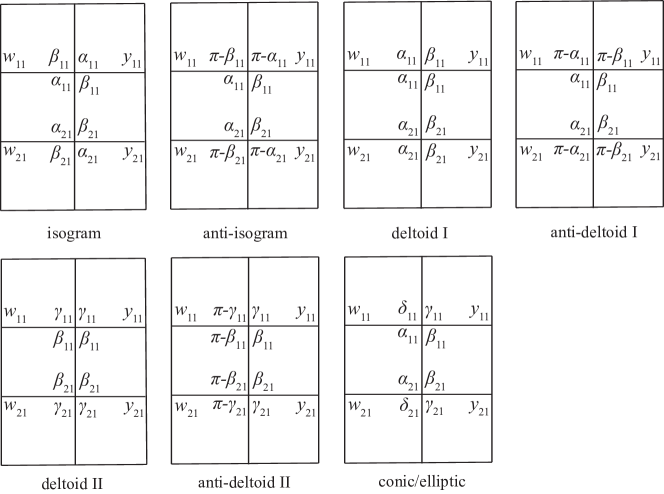
Figure 18: Labelling of proportional couplings.

anti-deltoid I

Similar to deltoid I:

$$\dfrac{\tan\alpha_{11}}{\tan\beta_{11}}=\dfrac{\tan\alpha_{21}}{\tan\beta_{21}}$$

The ratios are:

$$\begin{gathered}\dfrac{y_{21}}{y_{11}}=\dfrac{\cos\beta_{11}}{\cos\beta_{21}}\\ \dfrac{w_{21}}{w_{11}}=\dfrac{\cos\alpha_{11}}{\cos\alpha_{21}}~{}(\mathrm{let~{}}\alpha\rightarrow\beta,~{}\beta\rightarrow\alpha)\\ \dfrac{y_{31}}{y_{21}}=\dfrac{\cos\beta_{11}}{\cos\beta_{21}}~{}(\mathrm{let~{}}\alpha\rightarrow\pi-\alpha,~{}\beta\rightarrow\pi-\beta)\\ \dfrac{w_{31}}{w_{21}}=\dfrac{\cos\alpha_{11}}{\cos\alpha_{21}}~{}(\mathrm{let~{}}\alpha\rightarrow\pi-\beta,~{}\beta\rightarrow\pi-\alpha)\\ \end{gathered}$$

deltoid II

The proportional dependence $y_{21}=cy_{11}$ relies on vertices 11 and 21 to form a reducible coupling, i.e, the amplitudes being equal:

$$p^{x}_{11}=p^{x}_{21},~{}p^{x}=\sqrt{\dfrac{\sin^{2}\beta}{\sin^{2}\gamma}-1}~{}~{}\Leftrightarrow~{}~{}\dfrac{\sin\beta_{11}}{\sin\gamma_{11}}=\dfrac{\sin\beta_{21}}{\sin\gamma_{21}}$$

The ratios are:

$$\begin{gathered}\dfrac{y_{21}}{y_{11}}=\mathrm{sign}\left(\dfrac{\pi-\beta_{21}-\gamma_{21}}{\pi-\beta_{11}-\gamma_{11}}\right)\sqrt{\dfrac{\sin(\beta_{21}+\gamma_{21})\sin(\beta_{11}-\gamma_{11})}{\sin(\beta_{21}-\gamma_{21})\sin(\beta_{11}+\gamma_{11})}}\\ \dfrac{w_{21}}{w_{11}}=\dfrac{y_{21}}{y_{11}}\\ \dfrac{y_{31}}{y_{21}}=\dfrac{y_{21}}{y_{11}}~{}(\mathrm{let~{}}\beta\rightarrow\gamma,~{}\gamma\rightarrow\beta)\\ \dfrac{w_{31}}{w_{21}}=\dfrac{y_{21}}{y_{11}}~{}(\mathrm{let~{}}\beta\rightarrow\gamma,~{}\gamma\rightarrow\beta)\\ \end{gathered}$$

anti-deltoid II

Similar to deltoid II:

$$\dfrac{\sin\beta_{11}}{\sin\gamma_{11}}=\dfrac{\sin\beta_{21}}{\sin\gamma_{21}}$$

The ratios are the same with deltoid II ($y_{21}$ and $y_{11}$ changed to its opposite):

$$\begin{gathered}\dfrac{y_{21}}{y_{11}}=\mathrm{sign}\left(\dfrac{\pi-\beta_{21}-\gamma_{21}}{\pi-\beta_{11}-\gamma_{11}}\right)\sqrt{\dfrac{\sin(\beta_{21}+\gamma_{21})\sin(\beta_{11}-\gamma_{11})}{\sin(\beta_{21}-\gamma_{21})\sin(\beta_{11}+\gamma_{11})}}\\ \dfrac{w_{21}}{w_{11}}=\dfrac{\cos\alpha_{11}}{\cos\alpha_{21}}~{}(\mathrm{let~{}}\alpha\rightarrow\beta,~{}\beta\rightarrow\alpha)\\ \dfrac{y_{31}}{y_{21}}=\dfrac{\cos\beta_{11}}{\cos\beta_{21}}~{}(\mathrm{let~{}}\alpha\rightarrow\pi-\alpha,~{}\beta\rightarrow\pi-\beta)\\ \dfrac{w_{31}}{w_{21}}=\dfrac{\cos\alpha_{11}}{\cos\alpha_{21}}~{}(\mathrm{let~{}}\alpha\rightarrow\pi-\beta,~{}\beta\rightarrow\pi-\alpha)\\ \end{gathered}$$

conic

Two conic I or two conic IV form a proportional coupling if both the amplitudes and phase shifts are equal:

$$\begin{gathered}p^{x}_{11}=p^{x}_{21},~{}p^{x}=\sqrt{\dfrac{\sin\alpha\sin\beta}{\sin\gamma\sin\delta}-1}\\ \dfrac{\sin\beta_{11}\sin\delta_{11}}{\sin\alpha_{11}\sin\gamma_{11}}=\dfrac{\sin\beta_{21}\sin\delta_{21}}{\sin\alpha_{21}\sin\gamma_{21}}\end{gathered}$$

which leads to:

$$\dfrac{\sin\delta_{11}}{\sin\alpha_{11}}=\dfrac{\sin\delta_{21}}{\sin\alpha_{21}},~{}~{}\dfrac{\sin\beta_{11}}{\sin\gamma_{11}}=\dfrac{\sin\beta_{21}}{\sin\gamma_{21}}$$

The ratio for two conic I is:

$$\dfrac{y_{21}}{y_{11}}=\mathrm{sign}\left(\dfrac{\pi-\sigma_{21}}{\pi-\sigma_{11}}\right)\dfrac{p^{y}_{21}}{p^{y}_{11}}=\left.\mathrm{sign}\left(\dfrac{\pi-\sigma_{21}}{\pi-\sigma_{11}}\right)\sqrt{\dfrac{\sin\beta_{21}\sin\gamma_{21}}{\sin\delta_{21}\sin\alpha_{21}}-1}\middle/\sqrt{\dfrac{\sin\beta_{11}\sin\gamma_{11}}{\sin\delta_{11}\sin\alpha_{11}}-1}\right.$$

$$\dfrac{w_{21}}{w_{11}}=\left.\mathrm{sign}\left(\dfrac{\pi-\sigma_{21}}{\pi-\sigma_{11}}\right)\sqrt{\dfrac{\sin\delta_{21}\sin\alpha_{21}}{\sin\beta_{21}\sin\gamma_{21}}-1}\middle/\sqrt{\dfrac{\sin\delta_{11}\sin\alpha_{11}}{\sin\beta_{11}\sin\gamma_{11}}-1}\right.~{}(\mathrm{let~{}}\alpha\rightarrow\beta,~{}\beta\rightarrow\alpha,~{}\gamma\rightarrow\delta,~{}\delta\rightarrow\gamma)$$

$$\dfrac{y_{31}}{y_{21}}=\left.\mathrm{sign}\left(\dfrac{\pi-\sigma_{21}}{\pi-\sigma_{11}}\right)\sqrt{\dfrac{\sin\beta_{21}\sin\gamma_{21}}{\sin\delta_{21}\sin\alpha_{21}}-1}\middle/\sqrt{\dfrac{\sin\beta_{11}\sin\gamma_{11}}{\sin\delta_{11}\sin\alpha_{11}}-1}\right.~{}(\mathrm{let~{}}\alpha\rightarrow\delta,~{}\beta\rightarrow\gamma,~{}\gamma\rightarrow\beta,~{}\delta\rightarrow\alpha)$$

$$\dfrac{w_{31}}{w_{21}}=\left.\mathrm{sign}\left(\dfrac{\pi-\sigma_{21}}{\pi-\sigma_{11}}\right)\sqrt{\dfrac{\sin\delta_{21}\sin\alpha_{21}}{\sin\beta_{21}\sin\gamma_{21}}-1}\middle/\sqrt{\dfrac{\sin\delta_{11}\sin\alpha_{11}}{\sin\beta_{11}\sin\gamma_{11}}-1}\right.~{}(\mathrm{let~{}}\alpha\rightarrow\gamma,~{}\beta\rightarrow\delta,~{}\gamma\rightarrow\alpha,~{}\delta\rightarrow\beta)\\$$

$$\begin{gathered}\sigma=\alpha+\gamma=\beta+\delta,~{}~{}p^{y}=\sqrt{\dfrac{\sin\beta\sin\gamma}{\sin\delta\sin\alpha}-1}\end{gathered}$$

The ratio for two conic IV is:

$$\dfrac{y_{21}}{y_{11}}=\mathrm{sign}\left(\dfrac{\pi-\sigma_{11}}{\pi-\sigma_{21}}\right)\dfrac{p^{y}_{11}}{p^{y}_{21}}=\left.\mathrm{sign}\left(\dfrac{\pi-\sigma_{11}}{\pi-\sigma_{21}}\right)\sqrt{\dfrac{\sin\beta_{11}\sin\gamma_{11}}{\sin\delta_{11}\sin\alpha_{11}}-1}\middle/\sqrt{\dfrac{\sin\beta_{21}\sin\gamma_{21}}{\sin\delta_{21}\sin\alpha_{21}}-1}\right.$$

$$\dfrac{w_{21}}{w_{11}}=\left.\mathrm{sign}\left(\dfrac{\pi+\sigma_{11}}{\pi+\sigma_{21}}\right)\sqrt{\dfrac{\sin\delta_{11}\sin\alpha_{11}}{\sin\beta_{11}\sin\gamma_{11}}-1}\middle/\sqrt{\dfrac{\sin\delta_{21}\sin\alpha_{21}}{\sin\beta_{21}\sin\gamma_{21}}-1}\right.~{}(\mathrm{let~{}}\alpha\rightarrow\beta,~{}\beta\rightarrow\alpha,~{}\gamma\rightarrow\delta,~{}\delta\rightarrow\gamma)$$

$$\dfrac{y_{31}}{y_{21}}=\left.\mathrm{sign}\left(\dfrac{\pi+\sigma_{11}}{\pi+\sigma_{21}}\right)\sqrt{\dfrac{\sin\beta_{11}\sin\gamma_{11}}{\sin\delta_{11}\sin\alpha_{11}}-1}\middle/\sqrt{\dfrac{\sin\beta_{21}\sin\gamma_{21}}{\sin\delta_{21}\sin\alpha_{21}}-1}\right.~{}(\mathrm{let~{}}\alpha\rightarrow\delta,~{}\beta\rightarrow\gamma,~{}\gamma\rightarrow\beta,~{}\delta\rightarrow\alpha)$$

$$\dfrac{w_{31}}{w_{21}}=\left.\mathrm{sign}\left(\dfrac{\pi-\sigma_{11}}{\pi-\sigma_{21}}\right)\sqrt{\dfrac{\sin\delta_{11}\sin\alpha_{11}}{\sin\beta_{11}\sin\gamma_{11}}-1}\middle/\sqrt{\dfrac{\sin\delta_{21}\sin\alpha_{21}}{\sin\beta_{21}\sin\gamma_{21}}-1}\right.~{}(\mathrm{let~{}}\alpha\rightarrow\gamma,~{}\beta\rightarrow\delta,~{}\gamma\rightarrow\alpha,~{}\delta\rightarrow\beta)\\$$

$$\begin{gathered}\sigma=\dfrac{-\alpha+\beta-\gamma+\delta}{2}+\pi,~{}~{}p^{y}=\sqrt{\dfrac{\sin\beta\sin\gamma}{\sin\delta\sin\alpha}-1}\end{gathered}$$

elliptic

Two elliptic vertices form a proportional coupling if the elliptic modulus, amplitudes and phase shifts are equal:

$$\begin{gathered}p^{x}_{11}=p^{x}_{21},~{}p^{x}=\sqrt{\dfrac{\sin\alpha\sin\beta}{\sin(\sigma-\alpha)\sin(\sigma-\beta)}-1},~{}\sigma=\dfrac{\alpha+\beta+\gamma+\delta}{2}\\ M_{11}=M_{21},~{}M=\dfrac{\sin\alpha\sin\beta\sin\gamma\sin\delta}{\sin(\sigma-\alpha)\sin(\sigma-\beta)\sin(\sigma-\gamma)\sin(\sigma-\delta)}\\ \dfrac{\sin\alpha_{11}\sin\gamma_{11}}{\sin(\sigma_{11}-\alpha_{11})\sin(\sigma_{11}-\gamma_{11})}=\dfrac{\sin\alpha_{21}\sin\gamma_{21}}{\sin(\sigma_{21}-\alpha_{21})\sin(\sigma_{21}-\gamma_{21})}\end{gathered}$$

which leads to

$$\dfrac{\sin\alpha_{11}\sin\beta_{11}}{\sin(\sigma_{11}-\alpha_{11})\sin(\sigma_{11}-\beta_{11})}=\dfrac{\sin\alpha_{21}\sin\beta_{21}}{\sin(\sigma_{21}-\alpha_{21})\sin(\sigma_{21}-\beta_{21})}$$

$$\dfrac{\sin\gamma_{11}\sin\delta_{11}}{\sin(\sigma_{11}-\gamma_{11})\sin(\sigma_{11}-\delta_{11})}=\dfrac{\sin\gamma_{21}\sin\delta_{21}}{\sin(\sigma_{21}-\gamma_{21})\sin(\sigma_{21}-\delta_{21})}$$

$$\dfrac{\sin\alpha_{11}\sin\gamma_{11}}{\sin(\sigma_{11}-\alpha_{11})\sin(\sigma_{11}-\gamma_{11})}=\dfrac{\sin\alpha_{21}\sin\gamma_{21}}{\sin(\sigma_{21}-\alpha_{21})\sin(\sigma_{21}-\gamma_{21})}$$

The ratio is:

$$\dfrac{y_{21}}{y_{11}} =\mathrm{sign}\left(\dfrac{\pi-\sigma_{21}}{\pi-\sigma_{11}}\right)\dfrac{p^{y}_{21}}{p^{y}_{11}}$$

$$=\left.\mathrm{sign}\left(\dfrac{\pi-\sigma_{21}}{\pi-\sigma_{11}}\right)\sqrt{\dfrac{\sin\beta_{21}\sin\gamma_{21}}{\sin(\sigma_{21}-\beta_{21})\sin(\sigma_{21}-\gamma_{21})}-1}\middle/\sqrt{\dfrac{\sin\beta_{11}\sin\gamma_{11}}{\sin(\sigma_{11}-\beta_{11})\sin(\sigma_{11}-\gamma_{11})}-1}\right.$$

$$\begin{gathered}\dfrac{w_{21}}{w_{11}}=\left.\mathrm{sign}\left(\dfrac{\pi-\sigma_{21}}{\pi-\sigma_{11}}\right)\sqrt{\dfrac{\sin\delta_{21}\sin\alpha_{21}}{\sin(\sigma_{21}-\delta_{21})\sin(\sigma_{21}-\alpha_{21})}-1}\middle/\sqrt{\dfrac{\sin\delta_{11}\sin\alpha_{11}}{\sin(\sigma_{11}-\delta_{11})\sin(\sigma_{11}-\alpha_{11})}-1}\right.\\ (\mathrm{let~{}}\alpha\rightarrow\beta,~{}\beta\rightarrow\alpha,~{}\gamma\rightarrow\delta,~{}\delta\rightarrow\gamma)\end{gathered}$$

$$\begin{gathered}\dfrac{y_{31}}{y_{21}}=\left.\mathrm{sign}\left(\dfrac{\pi-\sigma_{21}}{\pi-\sigma_{11}}\right)\sqrt{\dfrac{\sin\beta_{21}\sin\gamma_{21}}{\sin(\sigma_{21}-\beta_{21})\sin(\sigma_{21}-\gamma_{21})}-1}\middle/\sqrt{\dfrac{\sin\beta_{11}\sin\gamma_{11}}{\sin(\sigma_{11}-\beta_{11})\sin(\sigma_{11}-\gamma_{11})}-1}\right.\\ (\mathrm{let~{}}\alpha\rightarrow\delta,~{}\beta\rightarrow\gamma,~{}\gamma\rightarrow\beta,~{}\delta\rightarrow\alpha)\end{gathered}$$

$$\begin{gathered}\dfrac{w_{31}}{w_{21}}=\left.\mathrm{sign}\left(\dfrac{\pi-\sigma_{21}}{\pi-\sigma_{11}}\right)\sqrt{\dfrac{\sin\delta_{21}\sin\alpha_{21}}{\sin(\sigma_{21}-\delta_{21})\sin(\sigma_{21}-\alpha_{21})}-1}\middle/\sqrt{\dfrac{\sin\delta_{11}\sin\alpha_{11}}{\sin(\sigma_{11}-\delta_{11})\sin(\sigma_{11}-\alpha_{11})}-1}\right.\\ (\mathrm{let~{}}\alpha\rightarrow\gamma,~{}\beta\rightarrow\delta,~{}\gamma\rightarrow\alpha,~{}\delta\rightarrow\beta)\end{gathered}$$

Appendix L Equimodular couplings of two-vertex systems

In Figure 12(d), we described a two-vertex system from $y_{11}$ to $y_{21}$. An equimodular coupling of such a degree-4 two-vertex system means that $y_{11}$ and $y_{21}$ are periodical functions over a parameter $t$ in the complexified configuration space, oscillating at the same frequency. $y_{11}$ and $y_{21}$ may differ in amplitude and phase shift.

Conic

(He et al., 2023, Section 17) To let $y_{11}$ and $y_{21}$ have the same frequency, we need to apply an equal amplitude condition:

$$p^{x}_{11}=p^{x}_{21},~{}~{}p^{x}=\sqrt{\dfrac{\sin\alpha\sin\beta}{\sin\gamma\sin\delta}-1}$$

This is also the condition for two conic II, III, IV vertices to be equimodular coupled.

Elliptic

(He et al., 2023, Section 21) To let $y_{11}$ and $y_{21}$ have the same frequency, we need to apply equal moduli and amplitude condition:

$$\begin{gathered}\begin{dcases}M_{11}=M_{21}\\ p^{x}_{11}=p^{x}_{21}\\ \end{dcases}\\ M=\dfrac{\sin\alpha\sin\beta\sin\gamma\sin\delta}{\sin(\sigma-\alpha)\sin(\sigma-\beta)\sin(\sigma-\gamma)\sin(\sigma-\delta)}\\ p^{x}=\sqrt{\dfrac{\sin\alpha\sin\beta}{\sin\gamma\sin\delta}-1}\end{gathered}$$

Finally, for an equimodular Kokotsakis quadrilateral stitched by two conic equimodular coupled two-vertex systems, the flexibility condition is:

Equal amplitude

$$\begin{gathered}\begin{dcases}p^{x}_{11}=p^{x}_{21}\\ p^{x}_{12}=p^{x}_{22}\\ p^{y}_{11}=p^{y}_{12}\\ p^{y}_{21}=p^{y}_{22}\end{dcases}\\ p^{x}=\sqrt{\dfrac{\sin\alpha\sin\beta}{\sin\gamma\sin\delta}-1},~{}~{}p^{y}=\sqrt{\dfrac{\sin\beta\sin\gamma}{\sin\delta\sin\alpha}-1}\end{gathered}$$

Equal phase shift

(detailed expression in He et al. (2023, Section 17))

$$\theta^{a}_{11}-\theta^{a}_{21}=\theta^{a}_{12}-\theta^{a}_{22}$$

for an equimodular Kokotsakis quadrilateral stitched by two elliptic equimodular coupled two-vertex systems, the flexibility condition is:

Equal amplitude

$$\begin{gathered}\begin{dcases}M_{11}=M_{21}=M_{12}=M_{22}\\ p^{x}_{11}=p^{x}_{21}\\ p^{x}_{12}=p^{x}_{22}\\ p^{y}_{11}=p^{y}_{12}\\ p^{y}_{21}=p^{y}_{22}\end{dcases}\\ p^{x}=\sqrt{\dfrac{\sin\alpha\sin\beta}{\sin\gamma\sin\delta}-1},~{}~{}p^{y}=\sqrt{\dfrac{\sin\beta\sin\gamma}{\sin\delta\sin\alpha}-1}\end{gathered}$$

Equal phase shift

(detailed expression in He et al. (2023, Section 21))

$$\theta^{a}_{11}-\theta^{a}_{21}=\theta^{a}_{12}-\theta^{a}_{22}$$

Appendix M Details for the examples in the main text

Using the repetitive stitching method described in the main text and the information provided in Sections K and L, one can create a large library of sector-angle-periodic patterns formed by the proportional couplings and equimodular couplings. Below we provide the constraints on the sector angles within a unit and ensure the flexibility of the entire pattern for the six examples presented in Figure 3 of the main text. The shape of each unit is provided in Figure 19. The flexibility of the entire pattern is guaranteed by the periodicity of sector angles, which ensures the flexibility of new Kokotsakis quadrilaterals generated in between units among the stitching process.

The exact solutions of each set of constraints is provided in the associated MATLAB application (He, 2024). These numerical solutions are verified from plotting the folding motion in the 3-dimensional space. The pattern is plotted from one input folding angle, all the sector angles and uniform input crease lengths. The above parameters are fully adjustable, providing significant freedom in shaping the quad-mesh rigid origami.

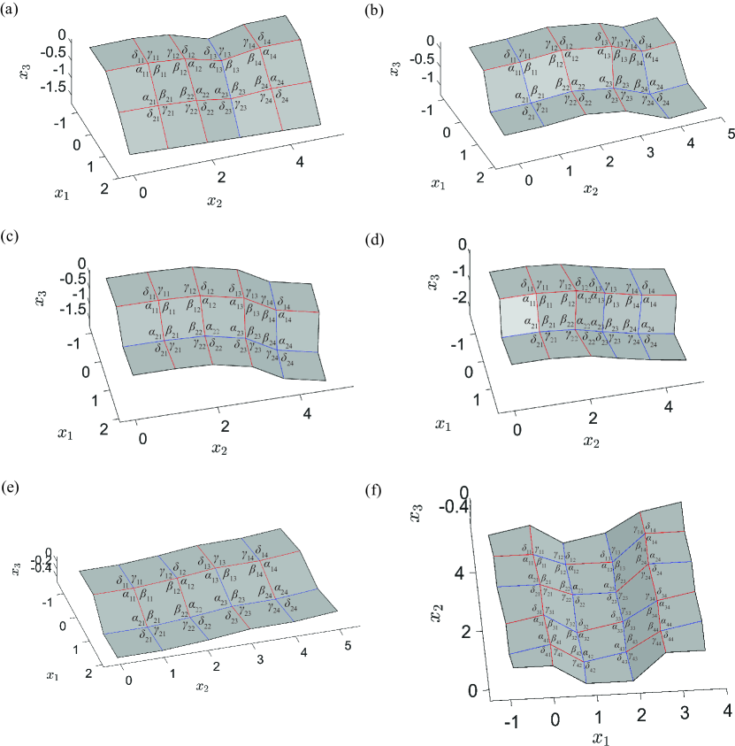
Figure 19: Labelling of sector angles and shapes of single units from (a) to (f) in Figure 3 of the main text.

Example 1, Figure 3(a), Figure 19(a), non-developable, proportional coupling

The unit size is $3\times 5$. A unit contains 8 interior vertices and 32 sector angles. The sector angles $\alpha_{ij},~{}\beta_{ij},~{}\gamma_{ij},~{}\delta_{ij}$, $i,~{}j\in\mathbb{Z}^{+},~{}i\leq 2,~{}j\leq 4$ meet the constraints below. There are 30 constraints for 32 sector angles, allowing two independent input sector angles. Columns 1 and 3 are isogram/eggbox vertices, columns 2 and 4 are deltoid I vertices.

Vertex type condition:

$$\begin{dcases}\gamma_{11}=\alpha_{11},~{}\delta_{11}=\beta_{11},~{}\gamma_{12}=\beta_{12},~{}\delta_{12}=\alpha_{12}\\ \gamma_{13}=\alpha_{13},~{}\delta_{13}=\beta_{13},~{}\gamma_{14}=\beta_{14},~{}\delta_{14}=\alpha_{14}\\ \gamma_{21}=\alpha_{21},~{}\delta_{21}=\beta_{21},~{}\gamma_{22}=\beta_{22},~{}\delta_{22}=\alpha_{22}\\ \gamma_{23}=\alpha_{23},~{}\delta_{23}=\beta_{23},~{}\gamma_{24}=\beta_{24},~{}\delta_{24}=\alpha_{24}\\ \end{dcases}$$

Planarity condition considering the periodicity of sector angles:

$$\begin{dcases}\beta_{11}+\beta_{21}+\beta_{12}+\beta_{12}=2\pi,~{}\gamma_{11}+\gamma_{21}+\gamma_{12}+\gamma_{12}=2\pi\\ \delta_{12}+\delta_{22}+\delta_{13}+\delta_{23}=2\pi,~{}\alpha_{12}+\alpha_{22}+\alpha_{13}+\alpha_{23}=2\pi\\ \beta_{13}+\beta_{23}+\beta_{14}+\beta_{14}=2\pi,~{}\gamma_{13}+\gamma_{23}+\gamma_{14}+\gamma_{14}=2\pi\\ \delta_{14}+\delta_{24}+\delta_{11}+\delta_{21}=2\pi,~{}\alpha_{14}+\alpha_{24}+\alpha_{11}+\alpha_{21}=2\pi\\ \end{dcases}$$

Condition for being proportional units:

$$\begin{dcases}\dfrac{\tan\beta_{12}}{\tan\alpha_{12}}=\dfrac{\tan\beta_{22}}{\tan\alpha_{22}}\\ \dfrac{\tan\beta_{14}}{\tan\alpha_{14}}=\dfrac{\tan\beta_{24}}{\tan\alpha_{24}}\\ \end{dcases}$$

Condition on equal ratio for proportional units:

$$\begin{dcases}\dfrac{\cos\dfrac{\alpha_{21}+\beta_{21}}{2}\cos\dfrac{\alpha_{11}-\beta_{11}}{2}}{\cos\dfrac{\alpha_{21}-\beta_{21}}{2}\cos\dfrac{\alpha_{11}+\beta_{11}}{2}}=\dfrac{\cos\beta_{22}}{\cos\beta_{12}}\\ \dfrac{\cos\beta_{22}}{\cos\beta_{12}}=\dfrac{\cos\dfrac{\alpha_{23}+\beta_{23}}{2}\cos\dfrac{\alpha_{13}-\beta_{13}}{2}}{\cos\dfrac{\alpha_{23}-\beta_{23}}{2}\cos\dfrac{\alpha_{13}+\beta_{13}}{2}}\\ \dfrac{\cos\dfrac{\alpha_{23}+\beta_{23}}{2}\cos\dfrac{\alpha_{13}-\beta_{13}}{2}}{\cos\dfrac{\alpha_{23}-\beta_{23}}{2}\cos\dfrac{\alpha_{13}+\beta_{13}}{2}}=\dfrac{\cos\beta_{24}}{\cos\beta_{14}}\\ \dfrac{\cos\beta_{24}}{\cos\beta_{14}}=\dfrac{\cos\dfrac{\alpha_{21}+\beta_{21}}{2}\cos\dfrac{\alpha_{11}-\beta_{11}}{2}}{\cos\dfrac{\alpha_{21}-\beta_{21}}{2}\cos\dfrac{\alpha_{11}+\beta_{11}}{2}}\end{dcases}$$

Example 2, Figure 3(b), Figure 19(b), non-developable, proportional coupling

The unit size is $3\times 5$. A unit contains 8 interior vertices and 32 sector angles. The sector angles $\alpha_{ij},~{}\beta_{ij},~{}\gamma_{ij},~{}\delta_{ij}$, $i,~{}j\in\mathbb{Z}^{+},~{}i\leq 2,~{}j\leq 4$ meet the constraints below. There are 29 constraints for 32 sector angles, allowing three independent input sector angles. Columns 1 and 3 are isogram/eggbox vertices, columns 2 and 4 are deltoid II vertices.

Vertex type condition:

$$\begin{dcases}\gamma_{11}=\alpha_{11},~{}\delta_{11}=\beta_{11},~{}\gamma_{12}=\delta_{12},~{}\beta_{12}=\alpha_{12}\\ \gamma_{13}=\alpha_{13},~{}\delta_{13}=\beta_{13},~{}\gamma_{14}=\delta_{14},~{}\beta_{14}=\alpha_{14}\\ \gamma_{21}=\alpha_{21},~{}\delta_{21}=\beta_{21},~{}\gamma_{22}=\delta_{22},~{}\beta_{22}=\alpha_{22}\\ \gamma_{23}=\alpha_{23},~{}\delta_{23}=\beta_{23},~{}\gamma_{24}=\delta_{24},~{}\beta_{24}=\alpha_{24}\\ \end{dcases}$$

Planarity condition considering the periodicity of sector angles:

$$\begin{dcases}\beta_{11}+\beta_{21}+\beta_{12}+\beta_{12}=2\pi,~{}\gamma_{11}+\gamma_{21}+\gamma_{12}+\gamma_{12}=2\pi\\ \delta_{12}+\delta_{22}+\delta_{13}+\delta_{23}=2\pi,~{}\alpha_{12}+\alpha_{22}+\alpha_{13}+\alpha_{23}=2\pi\\ \beta_{13}+\beta_{23}+\beta_{14}+\beta_{14}=2\pi,~{}\gamma_{13}+\gamma_{23}+\gamma_{14}+\gamma_{14}=2\pi\\ \delta_{14}+\delta_{24}+\delta_{11}+\delta_{21}=2\pi,~{}\alpha_{14}+\alpha_{24}+\alpha_{11}+\alpha_{21}=2\pi\\ \end{dcases}$$

Condition for being proportional units:

$$\begin{dcases}\dfrac{\sin\beta_{12}}{\sin\gamma_{12}}=\dfrac{\sin\beta_{22}}{\sin\gamma_{22}}\\ \dfrac{\sin\beta_{14}}{\sin\gamma_{14}}=\dfrac{\sin\beta_{24}}{\sin\gamma_{24}}\\ \end{dcases}$$

Condition on equal ratio for proportional units:

$$\begin{dcases}\dfrac{\cos\dfrac{\alpha_{21}+\beta_{21}}{2}\cos\dfrac{\alpha_{11}-\beta_{11}}{2}}{\cos\dfrac{\alpha_{21}-\beta_{21}}{2}\cos\dfrac{\alpha_{11}+\beta_{11}}{2}}=\mathrm{sign}\left(\dfrac{\pi-\beta_{22}-\gamma_{22}}{\pi-\beta_{12}-\gamma_{12}}\right)\sqrt{\dfrac{\sin(\beta_{22}+\gamma_{22})\sin(\beta_{12}-\gamma_{12})}{\sin(\beta_{22}-\gamma_{22})\sin(\beta_{12}+\gamma_{12})}}\\ \mathrm{sign}\left(\dfrac{\pi-\beta_{22}-\gamma_{22}}{\pi-\beta_{12}-\gamma_{12}}\right)\sqrt{\dfrac{\sin(\beta_{22}+\gamma_{22})\sin(\beta_{12}-\gamma_{12})}{\sin(\beta_{22}-\gamma_{22})\sin(\beta_{12}+\gamma_{12})}}=\dfrac{\cos\dfrac{\alpha_{23}+\beta_{23}}{2}\cos\dfrac{\alpha_{13}-\beta_{13}}{2}}{\cos\dfrac{\alpha_{23}-\beta_{23}}{2}\cos\dfrac{\alpha_{13}+\beta_{13}}{2}}\\ \dfrac{\cos\dfrac{\alpha_{23}+\beta_{23}}{2}\cos\dfrac{\alpha_{13}-\beta_{13}}{2}}{\cos\dfrac{\alpha_{23}-\beta_{23}}{2}\cos\dfrac{\alpha_{13}+\beta_{13}}{2}}=\mathrm{sign}\left(\dfrac{\pi-\beta_{24}-\gamma_{24}}{\pi-\beta_{14}-\gamma_{14}}\right)\sqrt{\dfrac{\sin(\beta_{24}+\gamma_{24})\sin(\beta_{14}-\gamma_{14})}{\sin(\beta_{24}-\gamma_{24})\sin(\beta_{14}+\gamma_{14})}}\end{dcases}$$

Note that the equation below can be inferred from the above three equations for equal ratio:

$$\mathrm{sign}\left(\dfrac{\pi-\beta_{24}-\gamma_{24}}{\pi-\beta_{14}-\gamma_{14}}\right)\sqrt{\dfrac{\sin(\beta_{24}+\gamma_{24})\sin(\beta_{14}-\gamma_{14})}{\sin(\beta_{24}-\gamma_{24})\sin(\beta_{14}+\gamma_{14})}}=\dfrac{\cos\dfrac{\alpha_{21}+\beta_{21}}{2}\cos\dfrac{\alpha_{11}-\beta_{11}}{2}}{\cos\dfrac{\alpha_{21}-\beta_{21}}{2}\cos\dfrac{\alpha_{11}+\beta_{11}}{2}}$$

Example 3, Figure 3(c), Figure 19(c), non-developable, proportional coupling

The unit size is $3\times 5$. A unit contains 8 interior vertices and 32 sector angles. The sector angles $\alpha_{ij},~{}\beta_{ij},~{}\gamma_{ij},~{}\delta_{ij}$, $i,~{}j\in\mathbb{Z}^{+},~{}i\leq 2,~{}j\leq 4$ meet the constraints below. There are 30 constraints for 32 sector angles, allowing two independent input sector angles. Columns 1 and 3 are deltoid I vertices, columns 2 and 4 are conic I vertices.

Vertex type condition:

$$\begin{dcases}\alpha_{11}=\delta_{11},~{}\beta_{11}=\gamma_{11},~{}\alpha_{13}=\delta_{13},~{}\beta_{13}=\gamma_{13}\\ \alpha_{21}=\delta_{21},~{}\beta_{21}=\gamma_{21},~{}\alpha_{23}=\delta_{23},~{}\beta_{23}=\gamma_{23}\\ \alpha_{12}+\gamma_{12}=\beta_{12}+\gamma_{12},~{}\alpha_{14}+\gamma_{14}=\beta_{14}+\gamma_{14}\\ \alpha_{22}+\gamma_{22}=\beta_{22}+\gamma_{22},~{}\alpha_{24}+\gamma_{24}=\beta_{24}+\gamma_{24}\\ \end{dcases}$$

Planarity condition considering the periodicity of sector angles:

$$\begin{dcases}\beta_{11}+\beta_{21}+\beta_{12}+\beta_{12}=2\pi,~{}\gamma_{11}+\gamma_{21}+\gamma_{12}+\gamma_{12}=2\pi\\ \delta_{12}+\delta_{22}+\delta_{13}+\delta_{23}=2\pi,~{}\alpha_{12}+\alpha_{22}+\alpha_{13}+\alpha_{23}=2\pi\\ \beta_{13}+\beta_{23}+\beta_{14}+\beta_{14}=2\pi,~{}\gamma_{13}+\gamma_{23}+\gamma_{14}+\gamma_{14}=2\pi\\ \delta_{14}+\delta_{24}+\delta_{11}+\delta_{21}=2\pi,~{}\alpha_{14}+\alpha_{24}+\alpha_{11}+\alpha_{21}=2\pi\\ \end{dcases}$$

Condition for being proportional units:

$$\begin{dcases}\dfrac{\tan\beta_{11}}{\tan\alpha_{11}}=\dfrac{\tan\beta_{21}}{\tan\alpha_{21}}\\ \dfrac{\tan\beta_{13}}{\tan\alpha_{13}}=\dfrac{\tan\beta_{23}}{\tan\alpha_{23}}\\ \dfrac{\sin\beta_{12}}{\sin\gamma_{12}}=\dfrac{\sin\beta_{22}}{\sin\gamma_{22}},~{}\dfrac{\sin\delta_{12}}{\sin\alpha_{12}}=\dfrac{\sin\delta_{22}}{\sin\alpha_{22}}\\ \dfrac{\sin\beta_{14}}{\sin\gamma_{14}}=\dfrac{\sin\beta_{24}}{\sin\gamma_{24}},~{}\dfrac{\sin\delta_{14}}{\sin\alpha_{14}}=\dfrac{\sin\delta_{24}}{\sin\alpha_{24}}\\ \end{dcases}$$

Condition on equal ratio for proportional units:

$$\begin{dcases}\dfrac{\cos\beta_{21}}{\cos\beta_{11}}=\left.\mathrm{sign}\left(\dfrac{\pi-\sigma_{22}}{\pi-\sigma_{12}}\right)\sqrt{\dfrac{\sin\beta_{22}\sin\gamma_{22}}{\sin\delta_{22}\sin\alpha_{22}}-1}\middle/\sqrt{\dfrac{\sin\beta_{12}\sin\gamma_{12}}{\sin\delta_{12}\sin\alpha_{12}}-1}\right.\\ \left.\mathrm{sign}\left(\dfrac{\pi-\sigma_{22}}{\pi-\sigma_{12}}\right)\sqrt{\dfrac{\sin\delta_{22}\sin\alpha_{22}}{\sin\beta_{22}\sin\gamma_{22}}-1}\middle/\sqrt{\dfrac{\sin\delta_{12}\sin\alpha_{12}}{\sin\beta_{12}\sin\gamma_{12}}-1}\right.=\dfrac{\cos\alpha_{23}}{\cos\alpha_{13}}\\ \dfrac{\cos\beta_{23}}{\cos\beta_{13}}=\left.\mathrm{sign}\left(\dfrac{\pi-\sigma_{24}}{\pi-\sigma_{14}}\right)\sqrt{\dfrac{\sin\beta_{24}\sin\gamma_{24}}{\sin\delta_{24}\sin\alpha_{24}}-1}\middle/\sqrt{\dfrac{\sin\beta_{14}\sin\gamma_{14}}{\sin\delta_{14}\sin\alpha_{14}}-1}\right.\\ \left.\mathrm{sign}\left(\dfrac{\pi-\sigma_{24}}{\pi-\sigma_{14}}\right)\sqrt{\dfrac{\sin\delta_{24}\sin\alpha_{24}}{\sin\beta_{24}\sin\gamma_{24}}-1}\middle/\sqrt{\dfrac{\sin\delta_{14}\sin\alpha_{14}}{\sin\beta_{14}\sin\gamma_{14}}-1}\right.=\dfrac{\cos\alpha_{21}}{\cos\alpha_{11}}\\ \end{dcases}$$

Example 4, Figure 3(d), Figure 19(d), non-developable, proportional coupling

The unit size is $3\times 5$. A unit contains 8 interior vertices and 32 sector angles. The sector angles $\alpha_{ij},~{}\beta_{ij},~{}\gamma_{ij},~{}\delta_{ij}$, $i,~{}j\in\mathbb{Z}^{+},~{}i\leq 2,~{}j\leq 4$ meet the constraints below. There are 30 constraints for 32 sector angles, allowing two independent input sector angles. Columns 1 and 3 are deltoid II vertices, columns 2 and 4 are conic I vertices.

Vertex type condition:

$$\begin{dcases}\beta_{11}=\alpha_{11},~{}\gamma_{11}=\delta_{11},~{}\beta_{13}=\alpha_{13},~{}\gamma_{13}=\delta_{13}\\ \beta_{21}=\alpha_{21},~{}\gamma_{21}=\delta_{21},~{}\beta_{23}=\alpha_{23},~{}\gamma_{23}=\delta_{23}\\ \alpha_{12}+\gamma_{12}=\beta_{12}+\gamma_{12},~{}\alpha_{14}+\gamma_{14}=\beta_{14}+\gamma_{14}\\ \alpha_{22}+\gamma_{22}=\beta_{22}+\gamma_{22},~{}\alpha_{24}+\gamma_{24}=\beta_{24}+\gamma_{24}\\ \end{dcases}$$

Planarity condition considering the periodicity of sector angles:

$$\begin{dcases}\beta_{11}+\beta_{21}+\beta_{12}+\beta_{12}=2\pi,~{}\gamma_{11}+\gamma_{21}+\gamma_{12}+\gamma_{12}=2\pi\\ \delta_{12}+\delta_{22}+\delta_{13}+\delta_{23}=2\pi,~{}\alpha_{12}+\alpha_{22}+\alpha_{13}+\alpha_{23}=2\pi\\ \beta_{13}+\beta_{23}+\beta_{14}+\beta_{14}=2\pi,~{}\gamma_{13}+\gamma_{23}+\gamma_{14}+\gamma_{14}=2\pi\\ \delta_{14}+\delta_{24}+\delta_{11}+\delta_{21}=2\pi,~{}\alpha_{14}+\alpha_{24}+\alpha_{11}+\alpha_{21}=2\pi\\ \end{dcases}$$

Condition for being proportional units:

$$\begin{dcases}\dfrac{\sin\beta_{11}}{\sin\gamma_{11}}=\dfrac{\sin\beta_{21}}{\sin\gamma_{21}}\\ \dfrac{\sin\beta_{13}}{\sin\gamma_{13}}=\dfrac{\sin\beta_{23}}{\sin\gamma_{23}}\\ \dfrac{\sin\beta_{12}}{\sin\gamma_{12}}=\dfrac{\sin\beta_{22}}{\sin\gamma_{22}},~{}\dfrac{\sin\delta_{12}}{\sin\alpha_{12}}=\dfrac{\sin\delta_{22}}{\sin\alpha_{22}}\\ \dfrac{\sin\beta_{14}}{\sin\gamma_{14}}=\dfrac{\sin\beta_{24}}{\sin\gamma_{24}},~{}\dfrac{\sin\delta_{14}}{\sin\alpha_{14}}=\dfrac{\sin\delta_{24}}{\sin\alpha_{24}}\\ \end{dcases}$$

Condition on equal ratio for proportional units:

$$\begin{dcases}\mathrm{sign}\left(\dfrac{\pi-\beta_{21}-\gamma_{21}}{\pi-\beta_{11}-\gamma_{11}}\right)\sqrt{\dfrac{\sin(\beta_{21}+\gamma_{21})\sin(\beta_{11}-\gamma_{11})}{\sin(\beta_{21}-\gamma_{21})\sin(\beta_{11}+\gamma_{11})}}\\ =\left.\mathrm{sign}\left(\dfrac{\pi-\sigma_{22}}{\pi-\sigma_{12}}\right)\sqrt{\dfrac{\sin\beta_{22}\sin\gamma_{22}}{\sin\delta_{22}\sin\alpha_{22}}-1}\middle/\sqrt{\dfrac{\sin\beta_{12}\sin\gamma_{12}}{\sin\delta_{12}\sin\alpha_{12}}-1}\right.\\ \left.\mathrm{sign}\left(\dfrac{\pi-\sigma_{22}}{\pi-\sigma_{12}}\right)\sqrt{\dfrac{\sin\delta_{22}\sin\alpha_{22}}{\sin\beta_{22}\sin\gamma_{22}}-1}\middle/\sqrt{\dfrac{\sin\delta_{12}\sin\alpha_{12}}{\sin\beta_{12}\sin\gamma_{12}}-1}\right.\\ =\mathrm{sign}\left(\dfrac{\pi-\beta_{23}-\gamma_{23}}{\pi-\beta_{13}-\gamma_{13}}\right)\sqrt{\dfrac{\sin(\beta_{23}+\gamma_{23})\sin(\beta_{13}-\gamma_{13})}{\sin(\beta_{23}-\gamma_{23})\sin(\beta_{13}+\gamma_{13})}}\\ \mathrm{sign}\left(\dfrac{\pi-\beta_{23}-\gamma_{23}}{\pi-\beta_{13}-\gamma_{13}}\right)\sqrt{\dfrac{\sin(\beta_{23}+\gamma_{23})\sin(\beta_{13}-\gamma_{13})}{\sin(\beta_{23}-\gamma_{23})\sin(\beta_{13}+\gamma_{13})}}\\ =\left.\mathrm{sign}\left(\dfrac{\pi-\sigma_{24}}{\pi-\sigma_{14}}\right)\sqrt{\dfrac{\sin\beta_{24}\sin\gamma_{24}}{\sin\delta_{24}\sin\alpha_{24}}-1}\middle/\sqrt{\dfrac{\sin\beta_{14}\sin\gamma_{14}}{\sin\delta_{14}\sin\alpha_{14}}-1}\right.\\ \left.\mathrm{sign}\left(\dfrac{\pi-\sigma_{24}}{\pi-\sigma_{14}}\right)\sqrt{\dfrac{\sin\delta_{24}\sin\alpha_{24}}{\sin\beta_{24}\sin\gamma_{24}}-1}\middle/\sqrt{\dfrac{\sin\delta_{14}\sin\alpha_{14}}{\sin\beta_{14}\sin\gamma_{14}}-1}\right.\\ =\mathrm{sign}\left(\dfrac{\pi-\beta_{21}-\gamma_{21}}{\pi-\beta_{11}-\gamma_{11}}\right)\sqrt{\dfrac{\sin(\beta_{21}+\gamma_{21})\sin(\beta_{11}-\gamma_{11})}{\sin(\beta_{21}-\gamma_{21})\sin(\beta_{11}+\gamma_{11})}}\\ \end{dcases}$$

Example 5, Figure 3(e), Figure 19(e), developable, proportional coupling

The unit size is $3\times 5$. A unit contains 8 interior vertices and 32 sector angles. The sector angles $\alpha_{ij},~{}\beta_{ij},~{}\gamma_{ij},~{}\delta_{ij}$, $i,~{}j\in\mathbb{Z}^{+},~{}i\leq 2,~{}j\leq 4$ meet the constraints below. There are 30 constraints for 32 sector angles, allowing two independent input sector angles. Columns 1 and 3 are anti-deltoid I vertices, columns 2 and 4 are conic IV vertices. This example is formed from switching certain strips of Example 3, transforming it from a non-developable pattern into a developable one. For a solution from Example 3, let

$$\alpha_{ij}\rightarrow\pi-\alpha_{ij},~{}~{}\gamma_{ij}\rightarrow\pi-\gamma_{ij}$$

Example 6, Figure 3(f), Figure 19(f), developable, equimodular coupling

Here we choose a $5\times 5$ unit as we have not searched a numerical solution when using a $3\times 5$ unit. The constraints below are listed assuming all the vertices are conic I, then transforming them to conic IV (developable) from switching certain strips — let

$$\alpha_{ij}\rightarrow\pi-\alpha_{ij},~{}~{}\gamma_{ij}\rightarrow\pi-\gamma_{ij}$$

A $5\times 5$ unit contains 16 interior vertices and 64 sector angles, the sector angles $\alpha_{ij},~{}\beta_{ij},~{}\gamma_{ij},~{}\delta_{ij}$, $i,~{}j\in\mathbb{Z}^{+},~{}i\leq 4,~{}j\leq 4$ meet the constraints below.

Vertex type condition (all the vertices are conic I):

$$\begin{dcases}\alpha_{11}+\gamma_{11}=\beta_{11}+\gamma_{11},~{}\alpha_{12}+\gamma_{12}=\beta_{12}+\gamma_{12}\\ \alpha_{13}+\gamma_{13}=\beta_{13}+\gamma_{13},~{}\alpha_{14}+\gamma_{14}=\beta_{14}+\gamma_{14}\\ \alpha_{21}+\gamma_{21}=\beta_{21}+\gamma_{21},~{}\alpha_{22}+\gamma_{22}=\beta_{22}+\gamma_{22}\\ \alpha_{23}+\gamma_{23}=\beta_{23}+\gamma_{23},~{}\alpha_{24}+\gamma_{24}=\beta_{24}+\gamma_{24}\\ \alpha_{31}+\gamma_{31}=\beta_{31}+\gamma_{31},~{}\alpha_{32}+\gamma_{32}=\beta_{32}+\gamma_{32}\\ \alpha_{33}+\gamma_{33}=\beta_{33}+\gamma_{33},~{}\alpha_{34}+\gamma_{34}=\beta_{34}+\gamma_{34}\\ \alpha_{41}+\gamma_{41}=\beta_{41}+\gamma_{41},~{}\alpha_{42}+\gamma_{42}=\beta_{42}+\gamma_{42}\\ \alpha_{43}+\gamma_{43}=\beta_{43}+\gamma_{43},~{}\alpha_{44}+\gamma_{44}=\beta_{44}+\gamma_{44}\\ \end{dcases}$$

Planarity condition considering the periodicity of sector angles:

$$\begin{dcases}\beta_{11}+\beta_{21}+\beta_{12}+\beta_{12}=2\pi,~{}\gamma_{21}+\gamma_{31}+\gamma_{22}+\gamma_{32}=2\pi\\ \beta_{31}+\beta_{41}+\beta_{32}+\beta_{42}=2\pi,~{}\gamma_{41}+\gamma_{11}+\gamma_{42}+\gamma_{12}=2\pi\\ \alpha_{12}+\alpha_{22}+\alpha_{13}+\alpha_{23}=2\pi,~{}\delta_{22}+\delta_{32}+\delta_{23}+\delta_{33}=2\pi\\ \alpha_{32}+\alpha_{42}+\alpha_{33}+\alpha_{43}=2\pi,~{}\delta_{42}+\delta_{12}+\delta_{43}+\delta_{13}=2\pi\\ \beta_{13}+\beta_{23}+\beta_{14}+\beta_{14}=2\pi,~{}\gamma_{23}+\gamma_{33}+\gamma_{24}+\gamma_{34}=2\pi\\ \beta_{33}+\beta_{43}+\beta_{34}+\beta_{44}=2\pi,~{}\gamma_{43}+\gamma_{13}+\gamma_{44}+\gamma_{14}=2\pi\\ \alpha_{14}+\alpha_{24}+\alpha_{11}+\alpha_{21}=2\pi,~{}\delta_{24}+\delta_{34}+\delta_{21}+\delta_{31}=2\pi\\ \alpha_{34}+\alpha_{44}+\alpha_{31}+\alpha_{41}=2\pi,~{}\delta_{44}+\delta_{14}+\delta_{41}+\delta_{11}=2\pi\\ \end{dcases}$$

Condition on equal amplitudes:

$$\begin{dcases}\dfrac{\sin\alpha_{11}\sin\beta_{11}}{\sin\gamma_{11}\sin\delta_{11}}=\dfrac{\sin\alpha_{21}\sin\beta_{21}}{\sin\gamma_{21}\sin\delta_{21}},~{}\dfrac{\sin\alpha_{21}\sin\beta_{21}}{\sin\gamma_{21}\sin\delta_{21}}=\dfrac{\sin\alpha_{31}\sin\beta_{31}}{\sin\gamma_{31}\sin\delta_{31}},~{}\dfrac{\sin\alpha_{31}\sin\beta_{31}}{\sin\gamma_{31}\sin\delta_{31}}=\dfrac{\sin\alpha_{41}\sin\beta_{41}}{\sin\gamma_{41}\sin\delta_{41}}\\ \dfrac{\sin\alpha_{12}\sin\beta_{12}}{\sin\gamma_{12}\sin\delta_{12}}=\dfrac{\sin\alpha_{22}\sin\beta_{22}}{\sin\gamma_{22}\sin\delta_{22}},~{}\dfrac{\sin\alpha_{22}\sin\beta_{22}}{\sin\gamma_{22}\sin\delta_{22}}=\dfrac{\sin\alpha_{32}\sin\beta_{32}}{\sin\gamma_{32}\sin\delta_{32}},~{}\dfrac{\sin\alpha_{32}\sin\beta_{32}}{\sin\gamma_{32}\sin\delta_{32}}=\dfrac{\sin\alpha_{42}\sin\beta_{42}}{\sin\gamma_{42}\sin\delta_{42}}\\ \dfrac{\sin\alpha_{13}\sin\beta_{13}}{\sin\gamma_{13}\sin\delta_{13}}=\dfrac{\sin\alpha_{23}\sin\beta_{23}}{\sin\gamma_{23}\sin\delta_{23}},~{}\dfrac{\sin\alpha_{23}\sin\beta_{23}}{\sin\gamma_{23}\sin\delta_{23}}=\dfrac{\sin\alpha_{33}\sin\beta_{33}}{\sin\gamma_{33}\sin\delta_{33}},~{}\dfrac{\sin\alpha_{33}\sin\beta_{33}}{\sin\gamma_{33}\sin\delta_{33}}=\dfrac{\sin\alpha_{43}\sin\beta_{43}}{\sin\gamma_{43}\sin\delta_{43}}\\ \dfrac{\sin\alpha_{14}\sin\beta_{14}}{\sin\gamma_{14}\sin\delta_{14}}=\dfrac{\sin\alpha_{24}\sin\beta_{24}}{\sin\gamma_{24}\sin\delta_{24}},~{}\dfrac{\sin\alpha_{24}\sin\beta_{24}}{\sin\gamma_{24}\sin\delta_{24}}=\dfrac{\sin\alpha_{34}\sin\beta_{34}}{\sin\gamma_{34}\sin\delta_{34}},~{}\dfrac{\sin\alpha_{34}\sin\beta_{34}}{\sin\gamma_{34}\sin\delta_{34}}=\dfrac{\sin\alpha_{44}\sin\beta_{44}}{\sin\gamma_{44}\sin\delta_{44}}\\ \dfrac{\sin\beta_{11}\sin\gamma_{11}}{\sin\delta_{11}\sin\alpha_{11}}=\dfrac{\sin\beta_{12}\sin\gamma_{12}}{\sin\delta_{12}\sin\alpha_{12}},~{}\dfrac{\sin\beta_{12}\sin\gamma_{12}}{\sin\delta_{12}\sin\alpha_{12}}=\dfrac{\sin\beta_{13}\sin\gamma_{13}}{\sin\delta_{13}\sin\alpha_{13}},~{}\dfrac{\sin\beta_{13}\sin\gamma_{13}}{\sin\delta_{13}\sin\alpha_{13}}=\dfrac{\sin\beta_{14}\sin\gamma_{14}}{\sin\delta_{14}\sin\alpha_{14}}\\ \dfrac{\sin\beta_{21}\sin\gamma_{21}}{\sin\delta_{21}\sin\alpha_{21}}=\dfrac{\sin\beta_{22}\sin\gamma_{22}}{\sin\delta_{22}\sin\alpha_{22}},~{}\dfrac{\sin\beta_{22}\sin\gamma_{22}}{\sin\delta_{22}\sin\alpha_{22}}=\dfrac{\sin\beta_{23}\sin\gamma_{23}}{\sin\delta_{23}\sin\alpha_{23}},~{}\dfrac{\sin\beta_{23}\sin\gamma_{23}}{\sin\delta_{23}\sin\alpha_{23}}=\dfrac{\sin\beta_{24}\sin\gamma_{24}}{\sin\delta_{24}\sin\alpha_{24}}\\ \dfrac{\sin\beta_{31}\sin\gamma_{31}}{\sin\delta_{31}\sin\alpha_{31}}=\dfrac{\sin\beta_{32}\sin\gamma_{32}}{\sin\delta_{32}\sin\alpha_{32}},~{}\dfrac{\sin\beta_{32}\sin\gamma_{32}}{\sin\delta_{32}\sin\alpha_{32}}=\dfrac{\sin\beta_{33}\sin\gamma_{33}}{\sin\delta_{33}\sin\alpha_{33}},~{}\dfrac{\sin\beta_{33}\sin\gamma_{33}}{\sin\delta_{33}\sin\alpha_{33}}=\dfrac{\sin\beta_{34}\sin\gamma_{34}}{\sin\delta_{34}\sin\alpha_{34}}\\ \dfrac{\sin\beta_{41}\sin\gamma_{41}}{\sin\delta_{41}\sin\alpha_{41}}=\dfrac{\sin\beta_{42}\sin\gamma_{42}}{\sin\delta_{42}\sin\alpha_{42}},~{}\dfrac{\sin\beta_{42}\sin\gamma_{42}}{\sin\delta_{42}\sin\alpha_{42}}=\dfrac{\sin\beta_{43}\sin\gamma_{43}}{\sin\delta_{43}\sin\alpha_{43}},~{}\dfrac{\sin\beta_{43}\sin\gamma_{43}}{\sin\delta_{43}\sin\alpha_{43}}=\dfrac{\sin\beta_{44}\sin\gamma_{44}}{\sin\delta_{44}\sin\alpha_{44}}\\ \end{dcases}$$

Regarding the condition on equal phase shifts for every Kokotsakis quadrilateral,

$$\begin{dcases}\theta^{a}_{11}-\theta^{a}_{21}=\theta^{a}_{12}-\theta^{a}_{22},~{}\theta^{a}_{21}-\theta^{a}_{31}=\theta^{a}_{22}-\theta^{a}_{32},~{}\theta^{a}_{31}-\theta^{a}_{41}=\theta^{a}_{32}-\theta^{a}_{42}\\ \theta^{b}_{12}-\theta^{b}_{22}=\theta^{b}_{13}-\theta^{b}_{23},~{}\theta^{b}_{22}-\theta^{b}_{32}=\theta^{b}_{23}-\theta^{b}_{33},~{}\theta^{b}_{32}-\theta^{b}_{42}=\theta^{b}_{33}-\theta^{b}_{43}\\ \theta^{a}_{13}-\theta^{a}_{23}=\theta^{a}_{14}-\theta^{a}_{24},~{}\theta^{a}_{23}-\theta^{a}_{33}=\theta^{a}_{24}-\theta^{a}_{34},~{}\theta^{a}_{33}-\theta^{a}_{43}=\theta^{a}_{34}-\theta^{a}_{44}\\ \end{dcases}$$

There are a total of 65 constraints on the 64 sector angles; however, Dieleman et al. (2020) reports a special solution to this system. If using $3\times 5$ unit, there are 29 constraints on the 32 sector angles, allowing three input angles, but we do not find a valid numerical solution.

Calculation of crease lengths

Plotting the entire pattern requires the calculation of all the crease lengths. As depicted in Figure 6, suppose the input crease lengths are located in row $i_{1}=0$ and column $i_{2}=0$, the first step is to rearrange the sector angles $\alpha,~{}\beta,~{}\gamma,~{}\delta$ to the angles $S^{\mathrm{a}},~{}S^{\mathrm{b}},~{}S^{\mathrm{c}},~{}S^{\mathrm{d}}$. Furthermore, for the right bottom region ($i_{1}>0$, $i_{2}>0$):

$$\begin{gathered}l_{x}(i,~{}j+1)=\dfrac{l_{x}(i,~{}j)\sin S^{\mathrm{a}}(i,~{}j)-l_{y}(i,~{}j)\sin(S^{\mathrm{d}}(i,~{}j)+S^{\mathrm{a}}(i,~{}j))}{\sin S^{\mathrm{b}}(i,~{}j)}\\ l_{y}(i+1,~{}j)=\dfrac{l_{y}(i,~{}j)\sin S^{\mathrm{c}}(i,~{}j)-l_{x}(i,~{}j)\sin(S^{\mathrm{d}}(i,~{}j)+S^{\mathrm{c}}(i,~{}j))}{\sin S^{\mathrm{b}}(i,~{}j)}\\ \end{gathered}$$

for the right top region ($i_{1}<0$, $i_{2}>0$):

$$\begin{gathered}l_{x}(i,~{}j+1)=\dfrac{l_{x}(i,~{}j)\sin S^{\mathrm{d}}(i,~{}j)-l_{y}(i+1,~{}j)\sin(S^{\mathrm{a}}(i,~{}j)+S^{\mathrm{d}}(i,~{}j))}{\sin S^{\mathrm{c}}(i,~{}j)}\\ l_{y}(i,~{}j)=\dfrac{l_{y}(i+1,~{}j)\sin S^{\mathrm{b}}(i,~{}j)-l_{x}(i,~{}j)\sin(S^{\mathrm{a}}(i,~{}j)+S^{\mathrm{b}}(i,~{}j))}{\sin S^{\mathrm{c}}(i,~{}j)}\\ \end{gathered}$$

for the left bottom region ($i_{1}>0$, $i_{2}<0$):

$$\begin{gathered}l_{x}(i,~{}j)=\dfrac{l_{x}(i,~{}j+1)\sin S^{\mathrm{b}}(i,~{}j)-l_{y}(i,~{}j)\sin(S^{\mathrm{c}}(i,~{}j)+S^{\mathrm{b}}(i,~{}j))}{\sin S^{\mathrm{a}}(i,~{}j)}\\ l_{y}(i+1,~{}j)=\dfrac{l_{y}(i,~{}j)\sin S^{\mathrm{d}}(i,~{}j)-l_{x}(i,~{}j+1)\sin(S^{\mathrm{c}}(i,~{}j)+S^{\mathrm{d}}(i,~{}j))}{\sin S^{\mathrm{a}}(i,~{}j)}\\ \end{gathered}$$

for the left top region ($i_{1}<0$, $i_{2}<0$)

$$\begin{gathered}l_{x}(i,~{}j)=\dfrac{l_{x}(i,~{}j+1)\sin S^{\mathrm{c}}(i,~{}j)-l_{y}(i+1,~{}j)\sin(S^{\mathrm{b}}(i,~{}j)+S^{\mathrm{c}}(i,~{}j))}{\sin S^{\mathrm{d}}(i,~{}j)}\\ l_{y}(i,~{}j)=\dfrac{l_{y}(i+1,~{}j)\sin S^{\mathrm{a}}(i,~{}j)-l_{x}(i,~{}j+1)\sin(S^{\mathrm{b}}(i,~{}j)+S^{\mathrm{a}}(i,~{}j))}{\sin S^{\mathrm{d}}(i,~{}j)}\\ \end{gathered}$$

Appendix N Evidences for limit smooth surface

In this section, we compile the available information regarding the limit smooth surface from refining quad-mesh rigid origami generated from repetitive stitching of proportional couplings and equimodular couplings. To the best of our knowledge, existing methods — namely, 1) the standard convergence theorem for conjugate nets (Section G), 2) the approach for V-hedra (Section I), and 3) the approach for T-hedra (Section J) — are not applicable. The reasons are as follows: 1) the new patterns are not based on a system of first-order partial difference equations; and 2) the sector angles, as well as the more sparsely constructed quad-meshes derived from vertices at the same relative periodic position across units, do not fall within the categories of V-hedra or T-hedra.

To tackle this challenge, we first observed the existence of zig-zag mode along one coordinate among all the examples. We conjecture that it will make limit smooth surface a ruled surface, no matter how the input crease length is distributed. For instance in Figure 20 below, $i_{1}$ is the ruling direction. This observation is numerically examined from calculating the coefficient of determination $R^{2}$ of linear regression for each column or row of vertices on the ruling direction. Specifically, $R^{2}$ is the ratio of the explained variance to the total variance calculated following the steps below. Let $x(i)=[x_{1}(i);~{}x_{2}(i);~{}x_{3}(i)]\in\mathbb{R}^{3},~{}i\in\mathbb{Z}_{+},~{}i\leq n,~{}n\in\mathbb{Z}_{+}$ be a data set of $n$ points in $\mathbb{R}^{3}$,

$$X=\begin{bmatrix}x(1)&x(2)&\cdots&x(n)\end{bmatrix}\mathrm{~{}is~{}a~{}}3\times n\mathrm{~{}coordinate~{}matrix}$$

$$\overline{X}=\begin{bmatrix}\left.\sum\limits_{i=1}^{n}x_{1}(i)\middle/n\right.\\ \left.\sum\limits_{i=1}^{n}x_{2}(i)\middle/n\right.\\ \left.\sum\limits_{i=1}^{n}x_{3}(i)\middle/n\right.\\ \end{bmatrix}\mathrm{~{}is~{}the~{}mean~{}value~{}of~{}coordinates}$$

$$\mathrm{d}X=\begin{bmatrix}x(1)-\overline{X}&x(2)-\overline{X}&\cdots&x(n)-\overline{X}\end{bmatrix}\mathrm{~{}is~{}the~{}residual}$$

$$C=\dfrac{\mathrm{d}X\mathrm{d}X^{\mathrm{T}}}{n-1}\mathrm{~{}is~{}the~{}}3\times 3\mathrm{~{}variance}-\mathrm{covariance~{}matrix}$$

Apply a spectral decomposition to $C$, $C=RDR^{\mathrm{T}}$. The direction of the best fit line is the first column $R(:,~{}1)$ of $R$. The line of best fit is hence $\overline{X}+tR(:,~{}1),~{}t\in\mathbb{R}$. The coefficient of determination is:

$$R^{2}=\dfrac{D(1,~{}1)}{\mathrm{trace}(D)}$$

The closer $R^{2}$ is to 1, the more closely the data aligns with a perfect linear relation. The result of minimum $R^{2}$ across all the rulings for all the examples are listed below:

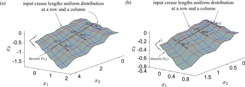
Figure 20: Illustration on the limit smooth surface for the quad-mesh rigid origami generated from repetitive stitching of proportional couplings and equimodular couplings.

Figure 2 in the main text

at folding angle $-30^{\circ}$

number of units	1	4	9	25	49
uniform input crease lengths	0.99852	0.99956	0.99979	0.99992	0.99996
quadratic input crease lengths	0.99869	0.99949	0.99976	0.99990	0.99995

Figure 3a in the main text

at folding angle $-60^{\circ}$

number of units	1	4	9	25	49
uniform input crease lengths	0.99636	0.99886	0.99945	0.99978	0.99988
quadratic input crease lengths	0.99700	0.99878	0.99939	0.99976	0.99987

Figure 3b in the main text

at folding angle $-30^{\circ}$

number of units	1	4	9	25	49
uniform input crease lengths	0.97546	0.99103	0.99540	0.99813	0.99899
quadratic input crease lengths	0.98050	0.99052	0.99490	0.99788	0.99885

Figure 3c in the main text

at folding angle $-30^{\circ}$

number of units	1	4	9	25	49
uniform input crease lengths	0.97569	0.99111	0.99545	0.99815	0.99900
quadratic input crease lengths	0.98063	0.99061	0.99495	0.99790	0.99886

Figure 3d in the main text

at folding angle $-30^{\circ}$

number of units	1	4	9	25	49
uniform input crease lengths	0.97257	0.98935	0.99423	0.99740	0.99846
quadratic input crease lengths	0.97825	0.98880	0.99361	0.99705	0.99825

Figure 3e in the main text

at folding angle $-30^{\circ}$

number of units	1	4	9	25	49
uniform input crease lengths	0.97576	0.99113	0.99545	0.99815	0.99900
quadratic input crease lengths	0.98068	0.99064	0.99496	0.99790	0.99886

Figure 3f in the main text

at folding angle $-30^{\circ}$

number of units	1	4	9	25	49
uniform input crease lengths	0.96847	0.98892	0.99484	0.99800	0.99895
quadratic input crease lengths	0.98123	0.98913	0.99448	0.99776	0.99881

On top of the ruled surface assumption, in Figure 20(a), where the input crease length distribution is uniform, we write the discrete surface in coordinate $i=(i_{1},~{}i_{2})\in\mathbb{Z}^{2}$:

$$x(i_{1},~{}i_{2})=\Gamma(i_{2})+i_{1}\Phi(i_{2})$$

Each $x(i_{1},~{}i_{2})$ is the location of vertex at the same relative position of unit $(i_{1},~{}i_{2})$. $\Gamma(i_{2})$ is the directrix. $\Phi(i_{2})$ is the ruling direction. There is no restriction on the choice of such representative vertex $x(i_{1},~{}i_{2})$. Further, let

$$\triangle\Gamma(i_{2})=\Gamma(i_{2}+1)-\Gamma(i_{2})$$

The periodicity of sector angles implies the periodicity of folding angles. As $\triangle\Gamma(i_{2})$ is a function over some sector angles, folding angles and input crease lengths on the directrix, and here the input crease lengths are uniformly distributed, we conclude that the directrix $\Gamma(i_{2})$ is a helical polyline. We could write $\triangle\Gamma(i_{2})$ in the form below, up to a rotation and translation:

$$\triangle\Gamma(i_{2})=\begin{bmatrix}a\cos(i_{2}+1)\theta\\ a\sin(i_{2}+1)\theta\\ b(i_{2}+1)\end{bmatrix}-\begin{bmatrix}a\cos i_{2}\theta\\ a\sin i_{2}\theta\\ bi_{2}\end{bmatrix}=\begin{bmatrix}-2a\sin\left(i_{2}\theta+\dfrac{\theta}{2}\right)\sin\dfrac{\theta}{2}\\[8.0pt] 2a\cos\left(i_{2}\theta+\dfrac{\theta}{2}\right)\sin\dfrac{\theta}{2}\\[8.0pt] b\end{bmatrix}$$

The parameter $a$ is the radius of the helix, $\theta$ and $b$ are the angular and height span of vertices on the helix. These parameters can be determined by the three-dimensional configuration of the pattern at any folded state.

Furthermore, the periodicity of sector and folding angles implies that the angle between $\triangle\Gamma(i_{2})$ and $\Phi(i_{2})$ is constant:

$$\dfrac{\triangle\Gamma(i_{2})\cdot\Phi(i_{2})}{\|\triangle\Gamma(i_{2})\|\|\Phi(i_{2})\|}=\mathrm{Const}\in[0,1).$$

Moreover, in Figure 20(b), for a generic distribution of input crease lengths, we introduce a distribution function $f(i_{2})$:

$$f(i_{2})=\dfrac{\|\triangle\Gamma(i_{2})\|}{\|\triangle\Gamma(0)\|}$$

Clearly $f(i_{2})\equiv 1$ corresponds to uniform input crease lengths. As the sector and folding angles remain periodic, we have

$$\triangle\Gamma(i_{2})=f(i_{2})\begin{bmatrix}-2a\sin\left(i_{2}\theta+\dfrac{\theta}{2}\right)\sin\dfrac{\theta}{2}\\[8.0pt] 2a\cos\left(i_{2}\theta+\dfrac{\theta}{2}\right)\sin\dfrac{\theta}{2}\\[8.0pt] b\end{bmatrix}$$

In conclusion, for any distribution of input crease lengths, the quad-mesh rigid origami (discrete surface) has the parametrization below:

$$x(i_{1},~{}i_{2})=\Gamma(0)+\sum\limits_{j=0}^{i_{2}}\triangle\Gamma(j)+i_{1}\Phi(i_{2})$$ (59)

Now as the mesh is arbitrarily refined, we conjecture that the repetitive stitching of units will converge to a smooth surface in the form below, up to a rotation and translation:

$$\begin{gathered}x(u_{1},~{}u_{2})=\Gamma(u_{2})+u_{1}\Phi(u_{2}),~{}~{}u_{1},~{}u_{2}\in\mathbb{R}\\ \Gamma(u_{2})=\Gamma(0)+\int\limits_{v=0}^{u_{2}}f(v)\begin{bmatrix}-a\sin v\\ a\cos v\\ b\end{bmatrix}\mathop{}\!\mathrm{d}v,~{}a>0,~{}b\in\mathbb{R}\\ f(u_{2})=\dfrac{\left\|\dfrac{\mathop{}\!\mathrm{d}\Gamma}{\mathop{}\!\mathrm{d}u_{2}}(u_{2})\right\|}{\left\|\dfrac{\mathop{}\!\mathrm{d}\Gamma}{\mathop{}\!\mathrm{d}u_{2}}(0)\right\|}\\ \Phi(u_{2})\in\mathbb{R}^{3},~{}||\Phi(u_{2})||\equiv 1\\ \dfrac{\dfrac{\mathop{}\!\mathrm{d}\Gamma}{\mathop{}\!\mathrm{d}u_{2}}\cdot\Phi}{f\sqrt{a^{2}+b^{2}}}=\mathrm{Const}\in[0,1)\end{gathered}$$ (60)

Here the directrix $\Gamma(u_{2})$ is a smooth curve, $f(u_{2})$ also becomes a smooth function. When $f(v)\equiv 1$, $\Gamma(u_{2})$ becomes a helix.

References

- Bauer et al. (2010) Ulrich Bauer, Konrad Polthier, and Max Wardetzky. Uniform Convergence of Discrete Curvatures from Nets of Curvature Lines. Discrete & Computational Geometry, 43(4):798–823, June 2010. ISSN 1432-0444. doi: 10.1007/s00454-009-9237-4.
- Bianchi (1890) Luigi Bianchi. Sopra alcune nuove classi di superficie e di sistemi tripli ortogonali. Annali di Matematica Pura ed Applicata (1867-1897), 18(1):301–358, 1890. Publisher: Springer.
- Blaschke (1923) Wilhelm Blaschke. Vorlesungen Über Differentialgeometrie und Geometrische Grundlagen von Einsteins Relativitätstheorie. Springer, Berlin, Heidelberg, 1923. ISBN 978-3-642-47125-4 978-3-642-47392-0. doi: 10.1007/978-3-642-47392-0.