Cubic-based Prediction Approach for Large Volatility Matrix using High-Frequency Financial Data

Sung Hoon Choi
Department of Economics, University of Connecticut, Storrs, CT 06269, USA. E-mail: sung_hoon.choi@uconn.edu.
   Donggyu Kim
Department of Economics, University of California, Riverside, CA 92521, USA. Email: donggyu.kim@ucr.edu.
Abstract

In this paper, we develop a novel method for predicting future large volatility matrices based on high-dimensional factor-based Itô processes. Several studies have proposed volatility matrix prediction methods using parametric models to account for volatility dynamics. However, these methods often impose restrictions, such as constant eigenvectors over time. To generalize the factor structure, we construct a cubic (order-3 tensor) form of an integrated volatility matrix process, which can be decomposed into low-rank tensor and idiosyncratic tensor components. To predict conditional expected large volatility matrices, we introduce the Projected Tensor Principal Orthogonal componEnt Thresholding (PT-POET) procedure and establish its asymptotic properties. Finally, the advantages of PT-POET are also verified by a simulation study and illustrated by applying minimum variance portfolio allocation using high-frequency trading data.

Key words: Diffusion process, low-rank, POET, projected PCA, semi-parametric tensor factor model.

1 Introduction

The analysis of volatility using high-frequency financial data is a vibrant research area in financial econometrics and statistics. In practice, understanding the dynamics of asset return volatility is essential for applications, such as hedging, option pricing, risk management, and portfolio optimization. The widespread availability of high-frequency financial data has led to the development of several effective non-parametric methods for estimating integrated volatility. Examples of these methods include two-time scale realized volatility (TSRV) (Zhang et al., 2005), multi-scale realized volatility (MSRV) (Zhang, 2006, 2011), pre-averaging realized volatility (PRV) (Christensen et al., 2010; Jacod et al., 2009), wavelet realized volatility (WRV) (Fan and Wang, 2007), kernel realized volatility (KRV) (Barndorff-Nielsen et al., 2008, 2011a), quasi-maximum likelihood estimator (QMLE) (Aït-Sahalia et al., 2010; Xiu, 2010), local method of moments (Bibinger et al., 2014), and robust pre-averaging realized volatility (Fan and Kim, 2018; Shin et al., 2023).

The incorporation of high-frequency data has significantly deepened our understanding of low-frequency (e.g., daily) market dynamics. Several conditional volatility models have been proposed based on realized volatility to capture these dynamics. Examples include realized volatility-based modeling approaches (Andersen et al., 2003), heterogeneous autoregressive (HAR) models (Corsi, 2009), high-frequency-based volatility (HEAVY) models (Shephard and Sheppard, 2010), realized GARCH models (Hansen et al., 2012), and unified GARCH-Itô models (Kim and Wang, 2016; Song et al., 2021). Their empirical studies typically focus on volatility dynamics given the high-frequency information for a finite number of assets. However, in practice, we often need to manage large portfolios, which causes the overparameterization issue due to the excessive number of parameters compared to the sample size. To address this issue, approximate factor model structures are commonly imposed on large volatility matrices (Fan et al., 2013). In particular, high-dimensional factor-based Itô processes are frequently used under sparsity assumptions on the idiosyncratic volatility (Ait-Sahalia and Xiu, 2017; Fan et al., 2016a; Fan and Kim, 2018; Kim et al., 2018). Recently, Kim and Fan (2019) proposed the factor GARCH-Itô model, and Shin et al. (2021) developed the factor and idiosyncratic VAR-Itô model, both based on high-dimensional factor-based Itô processes. These models assume that the eigenvalue sequence of latent factor volatility matrices follows either a unified GARCH-Itô structure (Kim and Wang, 2016) or a VAR structure, which allows the dynamics of volatility to be explained by factors. They restrict that the eigenvectors of the latent factor volatility matrices are time-invariant. However, several empirical studies have shown that eigenvectors are time-varying (Kong and Liu, 2018; Kong et al., 2023; Su and Wang, 2017). Thus, accommodating the eigenvector dynamics is important to better account for the dynamics of large volatility matrices.

This paper proposes a novel prediction approach for a future large volatility matrix. Specifically, we represent a large volatility matrix process in a cubic (order-3 tensor) form by stacking large integrated volatility matrices over time to capture interday time series dynamics. To address the high-dimensionality problem, we impose a low-rank factor structure (Chen and Fan, 2023; De Lathauwer et al., 2000; Kolda and Bader, 2009) and sparse idiosyncratic structure on the tensor. The low-rank tensor component represents a conditional expected factor volatility tensor, which follows a semiparametric factor structure (Chen et al., 2024). To implement the proposed integrated volatility matrix model, we use the Projected-PCA method suggested by Fan et al. (2016b) to estimate the time series loading matrix, which reflects the daily volatility dynamics. For example, we project the loading matrix onto a linear space spanned by past realized volatility estimators, which allows us to study the daily volatility dynamics and to predict the one-day-ahead large volatility matrix using current observed volatility information. To account for the sparse idiosyncratic volatility structure, after removing the projected factor volatility component, we adopt the principal orthogonal component thresholding (POET) (Fan et al., 2013) procedure. We refer to this method as the Projected Tensor POET (PT-POET) procedure. We then derive convergence rates for the projected integrated volatility matrix estimator and the predicted large volatility matrix using the PT-POET approach. In an empirical study, we demonstrate that the proposed PT-POET estimator performs well in out-of-sample predictions for the one-day-ahead large volatility matrix and in a minimum variance portfolio allocation analysis using high-frequency trading data.

The rest of the paper is organized as follows. Section 2 establishes the model and introduces the PT-POET method to predict the conditional expected large volatility matrix. Section 3 develops an asymptotic analysis of the PT-POET estimator. The merits of the proposed method are demonstrated by a simulation study in Section 4 and by real data application on predicting the one-day-ahead volatility matrix and portfolio allocation in Section 5. Section 6 concludes the study. All proofs are presented in Appendix A.

2 Model Setup and Estimation Procedure

Throughout this paper, we denote by $\|\mathbf{A}\|_{F}$, $\|\mathbf{A}\|_{2}$ (or $\|\mathbf{A}\|$ for short), $\|\mathbf{A}\|_{1}$, $\|\mathbf{A}\|_{\infty}$, and $\|\mathbf{A}\|_{\max}$ the Frobenius norm, operator norm, $l_{1}$-norm, $l_{\infty}$-norm, and elementwise norm, which are defined, respectively, as $\|\mathbf{A}\|_{F}=\mathrm{tr}^{1/2}(\mathbf{A}^{\prime}\mathbf{A})$, $\|\mathbf{A}\|=\lambda_{\max}^{1/2}(\mathbf{A}^{\prime}\mathbf{A})$, $\|\mathbf{A}\|_{1}=\max_{j}\sum_{i}|a_{ij}|$, $\|\mathbf{A}\|_{\infty}=\max_{i}\sum_{j}|a_{ij}|$, and $\|\mathbf{A}\|_{\max}=\max_{i,j}|a_{ij}|$. We use $\lambda_{\min}(\mathbf{A})$ and $\lambda_{\max}(\mathbf{A})$ to denote the minimum and maximum eigenvalues of a matrix $\mathbf{A}$. We denote by $\sigma_{i}(\mathbf{A})$ the $i$-th largest singular value of $\mathbf{A}$. When $\mathbf{a}$ is a vector, the maximum norm is denoted as $\|\mathbf{a}\|_{\infty}=\max_{i}|a_{i}|$, and both $\|\mathbf{a}\|$ and $\|\mathbf{a}\|_{F}$ are equal to the Euclidean norm.

For a tensor ${\cal A}\in\mathbb{R}^{I_{1}\times I_{2}\times I_{3}}$, we define its mode-1 matricization as a $I_{1}\times I_{2}I_{3}$ matrix $\mathcal{M}_{1}({\cal A})$ such that $[\mathcal{M}_{1}({\cal A})]_{i_{1},i_{2}+(i_{3}-1)I_{2}}=a_{i_{1}i_{2}i_{3}}$ for all $i_{1}\in[I_{1}],i_{2}\in[I_{2}],i_{3}\in[I_{3}]$. For a tensor $\mathcal{F}\in\mathbb{R}^{R_{1}\times R_{2}\times R_{3}}$ and a matrix $\mathbf{A}_{1}\in\mathbb{R}^{I_{1}\times R_{1}}$, the mode-1 product is a mapping defined as $\times_{1}:\mathbb{R}^{R_{1}\times R_{2}\times R_{3}}\times\mathbb{R}^{I_{1}\times R_{1}}\mapsto\mathbb{R}^{I_{1}\times R_{2}\times R_{3}}$ as $\mathcal{F}\times_{1}\mathbf{A}_{1}=[\sum_{r_{1}=1}^{R_{1}}a_{i_{1}r_{1}}f_{r_{1}r_{2}r_{3}}]_{i_{1}\in[I_{1}],r_{2}\in[R_{2}],r_{3}\in[R_{3}]}.$ Similarly, we can define mode matricization and mode product for mode-2 and mode-3, respectively.

2.1 A Model Setup

Denote by $\mathbf{X}^{l}(t)=(X^{l}_{1}(t),\dots,X^{l}_{p}(t))^{\top}$ the vector of true log-prices of $p$ assets at the $l$-th day and intraday time $t\in[0,1]$. To account for cross-sectional dependence, we consider the following factor-based jump diffusion model: for each $l=1,\dots,D$,

$$d\mathbf{X}^{l}(t)=\bm{\mu}^{l}(t)dt+\mathbf{B}^{l}(t)d\mathbf{f}^{l}(t)+d\mathbf{u}^{l}(t)+\mathbf{J}^{l}(t)d\bm{\Lambda}^{l}(t),$$ (2.1)

where $\bm{\mu}^{l}(t)\in\mathbb{R}^{p}$ is a drift vector, $\mathbf{B}^{l}(t)\in\mathbb{R}^{p\times r}$ is an unknown factor loading matrix, $\mathbf{f}^{l}(t)\in\mathbb{R}^{r}$ is a latent factor process, and $\mathbf{u}^{l}(t)$ is an idiosyncratic process. In addition, for the jump part, $\mathbf{J}^{l}(t)=(J_{1}(t),\dots,J_{p}(t))^{\top}$ is a jump size vector, and $\bm{\Lambda}^{l}(t)=(\Lambda^{l}_{1}(t),\dots,\Lambda^{l}_{p}(t))^{\top}$ is a $p$-dimensional Poisson process with an intensity vector $\mathbf{I}(t)=(I_{1}(t),\dots,I_{p}(t))^{\top}$. Assume that the latent factor and idiosyncratic processes $\mathbf{f}^{l}(t)$ and $\mathbf{u}^{l}(t)$ follow the continuous-time diffusion models as follows: for each $l=1,\dots,D$,

$$d\mathbf{f}^{l}(t)=\bm{\vartheta}^{l\top}(t)d\mathbf{W}^{l}(t)\text{ and }d\mathbf{u}^{l}(t)=\bm{\sigma}^{l\top}(t)d\mathbf{W}^{l*}(t),$$ (2.2)

where $\bm{\vartheta}^{l}(t)$ is an $r_{1}\times r_{1}$ matrix, $\bm{\sigma}^{l}(t)$ is a $p\times p$ matrix, $\mathbf{W}^{l}(t)$ and $\mathbf{W}^{l*}(t)$ are $r_{1}$-dimensional and $p$-dimensional independent Brownian motions, respectively.

Stochastic processes $\bm{\mu}^{l}(t),\mathbf{X}^{l}(t),\mathbf{f}^{l}(t),\mathbf{u}^{l}(t),\mathbf{B}^{l}(t),\bm{\sigma}^{l}(t)$ and $\bm{\vartheta}^{l}(t)$ are defined on a filtered probability space $(\Omega,{\cal I},{\cal I}_{t},t\in[0,\infty)\},P)$ with filtration ${\cal I}_{t}$ satisfying the usual conditions. We note that the time unit in our applications is the day, and high-frequency intra-daily asset data is observed. The instantaneous volatility of $\mathbf{X}^{l}(t)$ is

$$\bm{\gamma}^{l}(t)=(\gamma^{l}_{ij}(t))_{i,j=1,\dots,p}=\mathbf{B}^{l}(t)\bm{\vartheta}^{l\top}(t)\bm{\vartheta}^{l}(t)\mathbf{B}(t)^{l\top}+\bm{\sigma}^{l\top}(t)\bm{\sigma}^{l}(t),$$ (2.3)

and the integrated volatility for the $l$-th day is

$$\bm{\Gamma}_{l}=(\Gamma_{l,ij})_{i,j=1,\dots,p}=\int_{l-1}^{l}\bm{\gamma}^{l}(t)dt=\bm{\Psi}_{l}+\bm{\Sigma}_{l},$$ (2.4)

where $\bm{\Psi}_{l}=\int_{l-1}^{l}\mathbf{B}^{l}(t)\bm{\vartheta}^{l\top}(t)\bm{\vartheta}^{l}(t)\mathbf{B}(t)^{l\top}dt$ and $\bm{\Sigma}_{l}=\int_{l-1}^{l}\bm{\sigma}^{l\top}(t)\bm{\sigma}^{l}(t)dt$. For each $l=1,\dots,D$, the integrated volatility matrix $\bm{\Gamma}_{l}$ has the low-rank plus sparse structure (Ait-Sahalia and Xiu, 2017; Kim and Fan, 2019; Fan et al., 2008, 2013). Specifically, the factor volatility matrices $\bm{\Psi}_{l}$ has the finite rank $r_{1}$, and the idiosyncratic volatility matrices $\bm{\Sigma}_{l}=(\Sigma_{l,ij})_{i,j=1,\dots,p}$ is sparse as follows:

$\displaystyle\max_{1\leq l\leq D}\max_{1\leq i\leq p}\sum_{1\leq j\leq p}|\Sigma_{l,ij}|^{\eta}(\Sigma_{l,ii}\Sigma_{l,jj})^{(1-\eta)/2}=O(s_{p}),$ (2.5)

for some $\eta\in[0,1)$, the sparsity measure $s_{p}$ diverges slowly, such as $\log p$. We note that when $\eta=0$, $s_{p}$ measures the maximum number of non-zero elements in each row of $\bm{\Sigma}_{l}$.

We can write the integrated volatility matrix process of the model (2.4) in a cubic (order-3 tensor) form as follows:

$${\cal Y}=(\bm{\Gamma}_{l})_{l=1,\dots,D}={\cal F}\times_{1}\mathbf{Q}\times_{2}\mathbf{Q}\times_{3}\mathbf{V}+{\cal E}:={\cal S}+{\cal E},$$ (2.6)

where ${\cal Y}\in\mathbb{R}^{p\times p\times D}$, ${\cal F}$ is the $r_{1}\times r_{1}\times r_{2}$ latent tensor factor, $\mathbf{Q}=(q_{i,k_{1}})_{i=1,\dots,p,k_{1}=1,\dots,r_{1}}$ is the $p\times r_{1}$ loading matrix corresponds to the integrated volatility matrix, and $\mathbf{V}=(v_{l,k_{2}})_{l=1,\dots,D,k_{2}=1,\dots,r_{2}}$ is the $D\times r_{2}$ time series loading matrix corresponds to daily volatility dynamics. ${\cal S}$ is the factor volatility tensor, which has a Tucker decomposition such that $\mathbf{Q}$ and $\mathbf{V}$ are orthonormal matrices of the left singular vectors of ${\cal M}_{1}({\cal S})$ and ${\cal M}_{3}({\cal S})$, respectively. We refer to ${\cal E}=(\bm{\Sigma}_{l})_{l=1,\dots,D}$ as the idiosyncratic volatility tensor. We note that the time series loading matrix explains daily volatility dynamics, which are often driven by past realized volatilities (Corsi, 2009; Hansen et al., 2012; Kim and Fan, 2019; Kim and Wang, 2016; Shephard and Sheppard, 2010; Song et al., 2021). For instance, following the HAR model (Corsi, 2009), we can consider $v_{l,1}=b_{0}+b_{1}\zeta_{l-1}+b_{2}\frac{1}{5}\sum_{j=1}^{5}\zeta_{l-j}+b_{3}\frac{1}{21}\sum_{j=1}^{21}\zeta_{l-j}$, where $\zeta_{l}$ is the $l$-th day realized largest eigenvalue. This feature motivates the representation of the cubic structure in the model (2.6), and we propose a generalized model hereafter.

In this paper, our target is to predict the one-day-ahead integrated volatility matrix. In general, we assume that $v_{l,k_{2}}$ is ${\cal I}_{l-1}$-adapted and the idiosyncratic volatility matrices $\bm{\Sigma}_{l}$ are martingale processes such that $E(\bm{\Sigma}_{D+1}|{\cal I}_{D})=\bm{\Sigma}_{D}$ a.s. Thus, given the current information ${\cal I}_{D}$, we can predict the integrated volatility matrix as follows. The conditional expected large volatility matrix $\bm{\Gamma}_{D+1}$ is

$$E\left[\bm{\Gamma}_{D+1}|{\cal I}_{D}\right]={\cal F}\times_{1}\mathbf{Q}\times_{2}\mathbf{Q}\times_{3}\mathbf{v}_{D+1}+\bm{\Sigma}_{D}\text{ a.s.,}$$ (2.7)

where $\mathbf{v}_{D+1}:=(v_{D+1,1},\dots v_{D+1,k_{2}})$. Based on (2.4) and (2.6), we consider the following nonparametric structure on the time series loading components, which is modeled as additive via sieve approximations (Fan et al., 2016b): for each $k\leq r_{2}$ and $l\leq D$,

$\displaystyle v_{l,k}:=g_{k}(\mathbf{x}_{l})=\phi(\mathbf{x}_{l})^{\prime}\mathbf{a}_{k}+R_{k}(\mathbf{x}_{l}),$ (2.8)

where $\mathbf{x}_{l}=(x_{i1},\dots,x_{ld})$ is observable covariates that explain the time series loading vectors, $\phi(\mathbf{x}_{l})$ is a $(Jd)\times 1$ vector of basis functions, $\mathbf{a}_{k}$ is a $(Jd)\times 1$ vector of sieve coefficients, and $R_{k}(\mathbf{x}_{l})$ is the approximation error term. In this context, for example, $\mathbf{x}_{l}$ can be the past eigenvalues in the VAR model (Shin et al., 2021) or realized largest eigenvalues of the yesterday, last week, and last month in the HAR model (Corsi, 2009). We note that (2.8) can be written as $g_{k}(\mathbf{x}_{l})=\sum_{m=1}^{d}g_{km}(x_{lm})$, where $g_{km}(x_{lm})=\sum_{j=1}^{J}b_{j,km}\phi_{j}(x_{jm})+R_{km}(x_{jm})$. Hence, the additive component of $g_{k}$ can be estimated by the sieve method. We assume that $d$ is fixed, and the number of sieve terms $J$ grows very slowly as $D\rightarrow\infty$. In a matrix form, we can write

$\displaystyle\mathbf{V}:=\mathbf{G}(\mathbf{X})=\bm{\Phi}(\mathbf{X})\mathbf{A}+\mathbf{R}(\mathbf{X}),$ (2.9)

where the $D\times(Jd)$ matrix $\bm{\Phi}(\mathbf{X})=(\phi(\mathbf{x}_{1}),\dots,\phi(\mathbf{x}_{D}))^{\prime}$, the $(Jd)\times r_{2}$ matrix $\mathbf{A}=(\mathbf{a}_{1},\dots,\mathbf{a}_{r_{2}})$, and $\mathbf{R}(\mathbf{X})=(R_{k}(\mathbf{x}_{l}))_{D\times r_{2}}$.

The true underlined log-price $\mathbf{X}^{l}(t)$ in (2.1) cannot be observed because of the imperfections of the trading mechanisms. Hence, we assume that the high-frequency intraday observations are contaminated by microstructure noises:

$\displaystyle Y_{i}(t_{l,k})=X_{i}(t_{l,k})+u_{i}(t_{l,k}),\quad i=1,\dots,p,l=1,\dots,D,k=0,\dots,m,$ (2.10)

where $l-1=t_{l,0}<\cdots<t_{l,m}=l$, the microstructural noises are random variables with a mean of zero.

Several studies have developed a non-parametric integrated volatility matrix that is robust to jumps and dependent structures of the microstructure noise (Aït-Sahalia and Xiu, 2016; Barndorff-Nielsen et al., 2011b; Bibinger and Winkelmann, 2015; Jacod et al., 2009; Koike, 2016; Li and Linton, 2022; Shin et al., 2023). We can employ any well-performing realized volatility matrix estimator that satisfies Assumption 3.1 (v). In the numerical study, we utilize the jump-adjusted pre-averaging realized volatility matrix (PRVM) estimator (Aït-Sahalia and Xiu, 2016; Christensen et al., 2010; Jacod et al., 2009) as described in (4.1).

2.2 Projected Tensor POET

To utilize the semiparametric structure outlined in Section 2.1, it is necessary to project the time series loading vectors onto linear spaces spanned by the corresponding covariates. For this purpose, we apply the Projected-PCA (Fan et al., 2016b) procedure to the time series loading matrix with the well-performing integrated volatility tensor estimator. The specific procedure is as follows:

  1. 1.

    For each $l\leq D$, we estimate the integrated volatility matrix, $\bm{\Gamma}_{l}$, using a non-parametric estimation method with high-frequency log-price observations and denote them by $\widehat{\bm{\Gamma}}_{l}$. Let $\bar{\bm{\Psi}}_{l}=\sum_{i=1}^{r_{1}}\bar{\delta}_{l,i}\bar{\xi}_{l,i}\bar{\xi}_{l,i}^{\prime}$, where $\{\bar{\delta}_{l,i},\bar{\xi}_{l,i}\}_{i=1}^{p}$ are the eigenvalues and eigenvectors of $\widehat{\bm{\Gamma}}_{l}$ in decreasing order. Let $\widehat{{\cal Y}}=(\widehat{\bm{\Gamma}}_{l})_{l=1,\dots,D}$ and $\bar{{\cal S}}=(\bar{\bm{\Psi}}_{l})_{l=1,\dots,D}$, which are $p\times p\times D$ tensors.

  2. 2.

    Define the $D\times D$ projection matrix as $\mathbf{P}=\bm{\Phi}(\mathbf{X})(\bm{\Phi}(\mathbf{X})^{\prime}\bm{\Phi}(\mathbf{X}))^{-1}\bm{\Phi}(\mathbf{X})^{\prime}$. The columns $\widehat{\mathbf{Q}}$ are defined as the $r_{1}$ leading left singular vectors of ${\cal M}_{1}(\widetilde{{\cal S}})$, where $\widetilde{{\cal S}}=\bar{{\cal S}}\times_{3}\mathbf{P}$.

  3. 3.

    The columns $\widehat{\mathbf{V}}:=\widehat{\mathbf{G}}(\mathbf{X})$ are defined as the $r_{2}$ leading left singular vectors of the ${\cal M}_{3}(\widetilde{{\cal S}})$. Then, we can estimate $\mathbf{A}$ by

    $\displaystyle\widehat{\mathbf{A}}=(\widehat{\mathbf{a}}_{1},\dots,\widehat{\mathbf{a}}_{r_{2}})=(\bm{\Phi}(\mathbf{X})^{\prime}\bm{\Phi}(\mathbf{X}))^{-1}\bm{\Phi}(\mathbf{X})^{\prime}\widehat{\mathbf{G}}(\mathbf{X}).$

    Given any $\mathbf{x}\in{\cal X}$, we estimate $g_{k}(\cdot)$ by

    $$\widehat{g}_{k}(\mathbf{x})=\phi(\mathbf{x})^{\prime}\widehat{\mathbf{a}}_{k}\qquad\text{for}\quad k=1,\dots,r_{2},$$

    where ${\cal X}$ denotes the support of $\mathbf{x}_{i}$.

  4. 4.

    We estimate the latent tensor factor by

    $$\widehat{{\cal F}}=\widetilde{{\cal S}}\times_{1}\widehat{\mathbf{Q}}^{\top}\times_{2}\widehat{\mathbf{Q}}^{\top}\times_{3}\widehat{\mathbf{G}}(\mathbf{X})^{\top}.$$

    Then, we compute the principal orthogonal complement tensor as follows:

    $$\widehat{{\cal E}}=\widehat{{\cal Y}}-\widehat{{\cal S}},$$

    where the factor volatility tensor estimator $\widehat{{\cal S}}=\widehat{{\cal F}}\times_{1}\widehat{\mathbf{Q}}\times_{2}\widehat{\mathbf{Q}}\times_{3}\widehat{\mathbf{G}}(\mathbf{X})$.

  5. 5.

    Define $\widehat{{\cal E}}:=(\widetilde{\bm{\Sigma}}_{l})_{l=1,\dots,D}$. For each $l$, we apply the adaptive thresholding method to $\widetilde{\bm{\Sigma}}_{l}=(\widetilde{\Sigma}_{l,ij})_{1\leq i,j\leq p}$:

    $$\widehat{\bm{\Sigma}}_{l}=(\widehat{\Sigma}_{l,ij})_{1\leq i,j\leq p},\;\;\;\;\;\widehat{\Sigma}_{l,ij}=\left\{\begin{array}[]{ll}\widetilde{\Sigma}_{l,ij}\vee 0,&i=j\\ s_{ij}(\widetilde{\Sigma}_{l,ij})I(|\widetilde{\Sigma}_{l,ij}|\geq\tau_{ij}),&i\neq j\end{array}\right.,$$

    where an entry-dependent threshold $\tau_{ij}=\tau\sqrt{(\widetilde{\Sigma}_{l,ii}\vee 0)(\widetilde{\Sigma}_{l,jj}\vee 0)}$ and $s_{ij}(\cdot)$ is a generalized thresholding function (e.g., hard or soft thresholding; see Cai and Liu 2011; Rothman et al. 2009). The thresholding constant $\tau$ will be determined in Theorem 3.1.

  6. 6.

    Finally, we predict the conditional expected volatility matrix $E\left[\bm{\Gamma}_{D+1}|{\cal I}_{D}\right]$ by

    $$\widehat{\bm{\Gamma}}_{D+1}=\widehat{{\cal F}}\times_{1}\widehat{\mathbf{Q}}\times_{2}\widehat{\mathbf{Q}}\times_{3}\widehat{\mathbf{g}}(\mathbf{x}_{D+1})+\widehat{\bm{\Sigma}}_{D+1},$$

    where $\widehat{\mathbf{g}}(\mathbf{x}_{D+1})=(\widehat{g}_{1}(\mathbf{x}_{D+1}),\dots,\widehat{g}_{r_{2}}(\mathbf{x}_{D+1}))$ and $\widehat{\bm{\Sigma}}_{D+1}=\frac{1}{D}\sum_{l=1}^{D}\widehat{\bm{\Sigma}}_{l}$.

In summary, given the estimated integrated volatility tensor, we apply the Projected-PCA method (Fan et al., 2016b) to estimate the unknown nonparametric function using observable covariates, such as a series of past realized volatilities. Based on the projected tensor data, we then use tensor singular value decomposition to estimate loading matrices as well as the latent tensor factor. Then, we apply the thresholding method to the remaining residual component after removing the factor volatility tensor estimator. Finally, we predict the one-day-ahead realized volatility matrix by multiplying the estimated tensor factor and loading components, using the observable covariates $\mathbf{x}_{D+1}$, such as the realized volatility information on the $D$th day. We call this procedure the Projected Tensor Principal Orthogonal complEment Thresholding (PT-POET). The PT-POET method can accurately predict the factor volatility matrix by incorporating daily volatility dynamics via the projection approach based on the tensor structure. The numerical analyses in Sections 4 and 5 demonstrate that PT-POET performs well in predicting a one-day-ahead realized volatility matrix.

2.3 Choice of Tuning Parameters

To implement PT-POET, we need to determine tuning parameters $r_{1}$, $r_{2}$, and $J$. Several studies suggested data-driven methods to consistently estimate the number of factors by finding the largest singular value gap or singular value ratio (Ahn and Horenstein, 2013; Bai and Ng, 2002; Lam and Yao, 2012; Onatski, 2010). In this context, the rank of each dimension can be determined based on the matricized tensor (Chen et al., 2024). Specifically, $r_{1}$ and $r_{2}$ can be estimated as follows: for each $s\in\{1,3\}$, $\widehat{r}_{s}=\operatorname*{argmax}_{k\leq r_{\max}}(\sigma_{k}({\cal M}_{s}(\widehat{{\cal Y}}))-\sigma_{k+1}({\cal M}_{s}(\widehat{{\cal Y}})))$ or $\widehat{r}_{s}=\operatorname*{argmax}_{k\leq r_{\max}}\frac{\sigma_{k}({\cal M}_{s}(\widehat{{\cal Y}}))}{\sigma_{k+1}({\cal M}_{s}(\widehat{{\cal Y}}))}$ for a predetermined maximum number of factors $r_{\max}$. For the numerical studies in Sections 4 and 5, we employed $\widehat{r}_{1}=3$ and $\widehat{r}_{2}=1$ using the eigenvalue ratio method proposed by Ahn and Horenstein (2013) and the rank choice method considered in Ait-Sahalia and Xiu (2017).

Practitioners can flexibly choose the number of sieve terms, $J$, and the basis functions based on conjectures about the form of the nonparametric function (Chen et al., 2024; Fan et al., 2016b). In this paper, since the daily integrated volatility dynamic is a linear function of past realized volatilities, we employed an additive polynomial basis with a sieve dimension of $J=2$ for the numerical studies in Sections 4 and 5.

3 Asymptotic Properties

This section establishes the asymptotic properties of the proposed PT-POET estimator. To do this, we impose the following technical assumptions.

Assumption 3.1.
  • (i)

    Let $D_{\delta}=\min\{\widetilde{\delta}_{l,i}-\widetilde{\delta}_{l,i+1},i=1,\dots,r_{1},l=1,\dots,D\}$, where $\widetilde{\delta}_{l,i}$ is the leading eigenvalues of $\bm{\Psi}_{l}$ and $\widetilde{\delta}_{l,i+1}=0$. For some positive constant $C_{1}$, $D_{\delta}\geq C_{1}p$ a.s.

  • (ii)

    For some fixed constant $C_{2}$, we have

    $$\frac{p}{r_{1}}\max_{1\leq i\leq p}\sum_{j=1}^{r_{1}}\iota_{l,ij}^{2}\leq C_{2},$$

    where $\widetilde{\xi}_{l,j}=(\iota_{l,1j},\dots,\iota_{l,pj})^{\top}$ is the $j$th eigenvector of $\bm{\Psi}_{l}$ for each $l\leq D$.

  • (iii)

    For $k_{1}\leq r_{1}$ and $k_{2}\leq r_{2}$, the eigengap satisfies

    $\displaystyle|\sigma_{k_{1}}({\cal M}_{1}({\cal F}))-\sigma_{k_{1}+1}({\cal M}_{1}({\cal F}))|=O_{P}(p\sqrt{D}),$
    $\displaystyle|\sigma_{k_{2}}({\cal M}_{3}({\cal F}))-\sigma_{k_{2}+1}({\cal M}_{3}({\cal F}))|=O_{P}(p\sqrt{D}).$

    In addition, ${\cal M}_{m}({\cal F}){\cal M}_{m}^{\top}({\cal F})$ is a diagonal matrix with non-zero decreasing singular values for $m=1,2,3$.

  • (iv)

    There exist constants $c_{1},c_{2}>0$ such that $\lambda_{\min}(\bm{\Sigma}_{l})>c_{1}$ and $\|\bm{\Sigma}_{l}\|_{1}\leq c_{2}s_{p}$ for each $l\leq D$.

  • (v)

    The estimated nonparametric estimator $\widehat{\bm{\Gamma}}_{l}$ satisfies

    $$\Pr\Bigg{\{}\max_{1\leq l\leq D}\|\widehat{\bm{\Gamma}}_{l}-\bm{\Gamma}_{l}\|_{\max}\geq C\sqrt{\frac{\log(pD\vee m)}{m^{1/2}}}\Bigg{\}}\leq p^{-1},$$

    where $m$ is the number of observations of the process $\mathbf{X}$ each day.

Remark 3.1.

Assumption 3.1(i) and (ii) are the pervasive condition and incoherence condition for daily integrated volatility matrices, respectively. These assumptions are often imposed when analyzing the approximate factor models or the low-rank matrix inference (Ait-Sahalia and Xiu, 2017; Bai, 2003; Fan et al., 2013, 2018b; Kim and Fan, 2019; Stock and Watson, 2002). Assumption 3.1(ii) is the eigengap assumption for the tensor factor ${\cal F}$, which is essential for analyzing low-rank matrices (Candes and Plan, 2010; Cho et al., 2017; Fan et al., 2018a). Since we have a $p\times p\times D$ realized volatility tensor, the pervasive condition implies that the eigenvalue for the low-rank component has $p\sqrt{D}$ order based on the matricized tensor for each mode. To analyze large tensor inferences, we impose the element-wise convergence condition (Assumption 3.1(v)). This condition can be satisfied under the bounded instantaneous volatility condition (Tao et al., 2013). Furthermore, under the locally bounded condition of the instantaneous volatility process with heavy-tailed observations, we can obtain the element-wise convergence condition (Fan and Kim, 2018; Shin et al., 2021).

Assumption 3.2.
  • (i)

    There are $c_{\min}$ and $c_{\max}>0$ so that, with the probability approaching one, as $D\rightarrow\infty$,

    $$c_{\min}<\lambda_{\min}(D^{-1}\bm{\Phi}(\mathbf{X})^{\prime}\bm{\Phi}(\mathbf{X}))<\lambda_{\max}(D^{-1}\bm{\Phi}(\mathbf{X})^{\prime}\bm{\Phi}(\mathbf{X}))<c_{\max}.$$
  • (ii)

    $\max_{j\leq J,l\leq D,d^{\prime}\leq d}E\phi_{j}(x_{ld^{\prime}})^{2}<\infty$, and $\max_{k\leq r_{2},l\leq D}Eg_{k}(\mathbf{x}_{l})^{2}<\infty$.

Assumption 3.2 pertains to the basis functions. Intuitively, the strong law of large numbers implies Assumption 3.2(i), which can be satisfied by normalizing commonly used basis functions such as B-splines, polynomial series, or Fourier bases.

Assumption 3.3.

For all $d^{\prime}\leq d,k\leq r_{2}$,

  • (i)

    the functions $g_{kd^{\prime}}(\cdot)$ belong to a Hölder class $\mathcal{G}$ defined by, for some $L>0$,

    $\displaystyle\mathcal{G}=\{g:|g^{(c)}(s)-g^{(c)}(t)|\leq L|s-t|^{\alpha}\};$
  • (ii)

    the sieve coefficients $\{a_{j,kd^{\prime}}\}_{j\leq J}$ satisfy for $\kappa=2(c+\alpha)\geq 4$, as $J\rightarrow\infty$,

    $$\sup_{x\in\mathcal{X}_{d^{\prime}}}\left|g_{kd^{\prime}}(x)-\sum_{j=1}^{J}a_{j,kd^{\prime}}\phi_{s}(x)\right|^{2}=O(J^{-\kappa}/D),$$

    where $\mathcal{X}_{d}$ is the support of the $d^{\prime}$th element of $\mathbf{x}_{i}$;

  • (iii)

    $\max_{k\leq r_{2},j\leq J,d^{\prime}\leq d}a_{j,kd^{\prime}}^{2}=O(1/D)$.

Assumption 3.3 is related to the accuracy of the sieve approximation and can be satisfied using a common basis such as polynomial basis or B-splines (Chen, 2007).

We obtain the following elementwise convergence rates of the projected factor volatility matrix and sparse volatility matrix estimators.

Proposition 3.1.

Suppose that Assumptions 3.13.3 hold and $J=o(\sqrt{D})$. Let $\omega_{m}=m^{-\frac{1}{4}}\sqrt{J\log(pD\vee m)}+s_{p}\sqrt{J}/p+J^{\frac{1-\kappa}{2}}$ and $\tau\asymp\omega_{m}$. As $m,p,D,J\rightarrow\infty$, we have

$\displaystyle\max_{1\leq l\leq D}\|\widehat{\bm{\Psi}}_{l}-\bm{\Psi}_{l}\|_{\max}=O_{P}(\omega_{m}),$ (3.1)
$\displaystyle\max_{1\leq l\leq D}\|\widehat{\bm{\Sigma}}_{l}-\bm{\Sigma}_{l}\|_{\max}=O_{P}(\omega_{m}),\quad\max_{1\leq l\leq D}\|\widehat{\bm{\Sigma}}_{l}-\bm{\Sigma}_{l}\|=O_{P}(s_{p}\omega_{m}^{1-\eta}).$ (3.2)
Remark 3.2.

Proposition 3.1 represents that the projected factor and idiosyncratic volatility matrix estimators have the convergence rate $m^{-\frac{1}{4}}\sqrt{J}+\frac{\sqrt{J}}{p}+J^{\frac{1}{2}-\frac{\kappa}{2}}$ up to the log order and the sparsity level under the max norm. Specifically, $J$ relates to the sieve approximation, which accounts for the cost of approximating the unknown nonparametric function $g_{k}(\cdot)$. If $g_{k}(\cdot)$ is known, the rate of convergence is $m^{-\frac{1}{4}}+p^{-\frac{1}{2}}$ up to the log order and the sparsity level, which is similar to that of Kim and Fan (2019). The term $m^{-1/4}$ reflects the cost of estimating the unobserved integrated volatility matrix using high-frequency data, which is the optimal rate for the instantaneous volatility estimator in the presence of microstructure noise. The term $p^{-1/2}$ represents the cost of identifying the latent factor volatility.

The following theorem provides the convergence rate of the future volatility matrix estimator using the PT-POET method.

Theorem 3.1.

Suppose that Assumptions 3.13.3 hold and $J=o(\sqrt{D})$. Let $\delta_{m,p,D}=(m^{-\frac{1}{4}}J\sqrt{\log(pD\vee m)}+s_{p}J/p+J^{1-\frac{\kappa}{2}})\max_{j\leq J}\sup_{x}|\phi_{j}(x)|$, $\omega_{m}=m^{-\frac{1}{4}}\sqrt{J\log(pD\vee m)}+s_{p}\sqrt{J}/p+J^{\frac{1-\kappa}{2}}$ and $\tau\asymp\omega_{m}$. As $m,p,D,J\rightarrow\infty$, we have

$\displaystyle\|\widehat{\bm{\Gamma}}_{D+1}-E(\bm{\Gamma}_{D+1}|{\cal I}_{D})\|_{\max}=O_{P}(\delta_{m,p,D}),$ (3.3)
$\displaystyle\|\widehat{\bm{\Gamma}}_{D+1}-E(\bm{\Gamma}_{D+1}|{\cal I}_{D})\|_{\bm{\Gamma}^{*}}=O_{P}\left(\delta_{m,p,D}+\frac{s_{p}}{\sqrt{p}}+\sqrt{p}\delta_{m,p,D}^{2}+s_{p}\omega_{m}^{1-\eta}\right),$ (3.4)

where the relative Frobenius norm $\|\mathbf{A}\|_{\bm{\Gamma}^{*}}^{2}=p^{-1}\|\bm{\Gamma}^{*-1/2}\mathbf{A}\bm{\Gamma}^{*-1/2}\|_{F}^{2}$ and $\bm{\Gamma}^{*}=E(\bm{\Gamma}_{D+1}|{\cal I}_{D})$.

Remark 3.3.

Theorem 3.1 represents that PT-POET consistently predicts the conditional expected volatility matrix under both the max and relative Frobenius norms. As discussed in Remark 3.2, there are $m^{-1/4}$, $\sqrt{J}/P$, and $J$ terms. We note that out-of-sample predictions with any covariates $\mathbf{x}$ require additional costs such as $\sqrt{J}$ and the supremum term $\max_{j\leq J}\sup_{x}|\phi_{j}(x)|$, whereas the result in Proposition 3.1 does not require these costs since it pertains to in-sample prediction. Under the relative Frobenius norm, the additional term $s_{p}/\sqrt{p}$ arises from estimating the factor component, while the term $s_{p}\omega_{m}^{1-\eta}$ results from estimating the sparse idiosyncratic component.

4 Simulation Study

In this section, we conducted a simulation study to examine the finite sample performances of the proposed PT-POET method. We first generated the log-prices $\mathbf{X}^{l}(t_{j})$ for $D+1$ days with frequency $1/m$ on each day as follows: for $l=1,\dots,D+1$, $j=0,\dots,m$, and $t_{j}=j/m$,

$\displaystyle\mathbf{Y}^{l}(t_{j})=\mathbf{X}^{l}(t_{j})+\mathbf{e}^{l}(t_{j}),$
$\displaystyle d\mathbf{X}^{l}(t)=\bm{\psi}^{l\top}d\mathbf{W}(t)+\bm{\sigma}^{l\top}d\mathbf{W}^{*}(t)+\mathbf{J}^{l}(t)d\bm{\Lambda}^{l}(t),$

where we set the market microstructure noise as $\mathbf{e}^{l}(t_{j})=(e^{l}_{1}(t_{j}),\dots,e^{l}_{p}(t_{j}))$, where $e^{l}_{i}(t_{j})$ were from i.i.d. normal distribution with mean zero and standard deviation $0.01\sqrt{\Sigma_{ii}}$ for the $i$th asset, and the initial values $\mathbf{X}_{0}=(0,\dots,0)^{\top}$; $\mathbf{W}(t)$ and $\mathbf{W}^{*}(t)$ are $r$-dimensional and $p$-dimensional independent Brownian motions, respectively, $\mathbf{J}^{l}(t)=(J_{1}^{l}(t),\dots,J_{p}^{l}(t))^{\top}$ is the jump size vector, and $\bm{\Lambda}^{l}(t)=(\Lambda^{l}_{1}(t),\dots,\Lambda^{l}_{p}(t))^{\top}$ is the Poission process with intensity $\mathbf{I}(t)=(5,\dots,5)^{\top}$. The jump size $J_{i}^{l}(t)$ was obtained from the independent Gaussian distribution with mean zero and standard deviation $0.05\sqrt{\int_{0}^{1}\gamma_{ii}(t)dt}$. $\bm{\psi}^{l}$ and $\bm{\sigma}^{l}$ are the Cholesky decompositions of $\bm{\Psi}_{l}$ and $\bm{\Sigma}_{l}$, respectively, where the integrated volatility process components ${\cal S}=(\bm{\Psi}_{l})_{l=1,\dots,D+1}$ and ${\cal E}=(\bm{\Sigma}_{l})_{l=1,\dots,D+1}$ were constructed as follows:

$\displaystyle{\cal Y}={\cal S}+{\cal E}={\cal F}\times_{1}\mathbf{Q}\times_{2}\mathbf{Q}\times_{3}\mathbf{V}+{\cal E},$

where the $r_{1}\times r_{1}\times r_{2}$ latent tensor factor ${\cal F}$ and the $p\times r_{1}$ loading matrix $\mathbf{Q}$ were generated from the first $r_{1}$ leading eigenvalues and eigenvectors of $AA^{\prime}$, respectively, where each element of $A$ was taken from an i.i.d standard normal distribution; $\mathbf{V}=(v_{1},\dots,v_{D+1})^{\prime}$ was generated by $v_{l}=b_{0}+b_{1}v_{l-1}+b_{2}\frac{1}{5}\sum_{s=1}^{5}v_{l-s}+b_{3}\frac{1}{21}\sum_{s=1}^{21}v_{l-s}+\zeta_{l}$, where $\zeta_{l}\sim\mathcal{N}(0,1)$. The model parameters were set to be $b_{0}=0.5,b_{1}=0.372,b_{2}=0.343,b_{3}=0.224$. We set ranks $r_{1}=3$ and $r_{2}=1$, $p=200$.

We obtained the sparse volatility component ${\cal E}=(\bm{\Sigma}_{l})_{l=1,\dots,D+1}$ as follows: let $\mathbf{d}=\mathrm{diag}(d_{1}^{2},\dots,d_{p}^{2})$, where each $\{d_{i}\}$ was generated independently from Gamma $(\alpha,\beta)$ with $\alpha=\beta=100$. We set $s=(s_{1},\dots,s_{p})^{\prime}$ to be a sparse vector, where each $s_{i}$ was drawn from $\mathcal{N}(0,1)$ with probability $\frac{0.3}{\sqrt{p}\log{p}}$, and $s_{i}=0$ otherwise. Then, we set a sparse error covariance matrix as $\bm{\Sigma}=\mathbf{d}+ss^{\prime}-\mathrm{diag}\{s_{1}^{2},\dots,s_{p}^{2}\}$, and we let $\bm{\Sigma}_{l}=\bm{\Sigma}$ for each $l$. In the simulation, we generated $\bm{\Sigma}$ until it is positive definite. We first generated high-frequency data with $m=\{250,500,2000\}$ for 200 consecutive days, and we used the subsampled log prices of the last $D$ days. We varied $D$ from 50 to 200, and the whole simulation procedure was repeated 500 times.

To estimate the integrated volatility matrices, we employed the pre-averaging realized volatility matrix (PRVM) estimator $\widehat{\bm{\Gamma}}_{l}=(\widehat{\Gamma}_{l,ij})_{1\leq i,j\leq p}$ (Aït-Sahalia and Xiu, 2016; Christensen et al., 2010; Jacod et al., 2009) for each $l$-th day as follows:

$$\widehat{\Gamma}_{l,ij}=\frac{1}{\phi K}\sum_{k=1}^{m-K+1}\left\{\bar{Y}^{l}_{i}(t_{k})\bar{Y}^{l}_{j}(t_{k})-\frac{1}{2}\widehat{Y}^{l}_{i,j}(t_{k})\right\}\mathbf{1}\left\{\left|\bar{Y}^{l}_{i}(t_{k})\right|\leq u_{i,m}\right\}\mathbf{1}\left\{\left|\widetilde{Y}^{l}_{j}(t_{k})\right|\leq u_{j,m}\right\},$$ (4.1)

where

$\displaystyle\bar{Y}^{l}_{i}(t_{k})=\sum_{s=1}^{K-1}g\left(\frac{s}{K}\right)(Y^{l}_{i}(t_{k+s})-Y^{l}_{i}(t_{k+s-1})),$
$\displaystyle\widehat{Y}^{l}_{i,j}(t_{k})=\sum_{s=1}^{K}\Bigg{[}\left\{g\left(\frac{s}{K}\right)-g\left(\frac{s-1}{K}\right)\right\}^{2}$
$\displaystyle\qquad\qquad\qquad\qquad\times(Y^{l}_{i}(t_{k+s-1})-Y^{l}_{i}(t_{k+s-2}))(Y^{l}_{j}(t_{k+s-1})-Y^{l}_{j}(t_{k+s-2}))\Bigg{]},$

where $\phi=\int_{0}^{1}g(t)^{2}\,dt$, $\mathbf{1}\{\}$ is an indicator function, and $u_{i,m}=c_{i,u}m^{0.235}$ is a truncation parameter for some constant $c_{i,u}$. We chose the bandwidth parameter $K=\lfloor m^{1/2}\rfloor$, weight function $g(x)=x\wedge(1-x)$, and $c_{i,u}$ as 7 times the sample standard deviation for the pre-averaged variables $m^{\frac{1}{4}}\bar{Y}_{i}(t_{d,k})$.

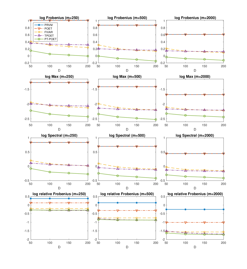
With the aggregated volatility matrix estimates spanning $D$ days, $\widehat{{\cal Y}}=(\widehat{\bm{\Gamma}}_{l})_{l=1,\dots,D}$, we examined the out-of-sample performance of predicting the one-day-ahead aggregated volatility matrix. For comparison, the PRVM, POET, FIVAR, T-POET, and PT-POET methods were employed to predict $E(\bm{\Gamma}_{D+1}|{\cal I}_{D})$, given the past $D$ period observation. In particular, for PT-POET, we utilized the past daily, weekly, and monthly averages of the top eigenvalues for $\mathbf{X}$ with the additive polynomial basis and $J=2$. PRVM and POET represent the PRVM estimator (i.e., $\widehat{\bm{\Sigma}}_{D}$) and the POET estimator (Fan et al., 2013) based on PRVM at the $D$th day, respectively. We also employed the FIVAR method (Shin et al., 2021) to model the factor part dynamics based on the PRVM estimator. Specifically, we used the past $D$ days observations to estimate the model parameters and the previous 21 days to estimate the time-invariant eigenvectors. We do not model the idiosyncratic dynamics to compare the performance of the factor modeling. Details can be found in Shin et al. (2021). T-POET represents the $D$th day matrix estimator based on the conventional estimation procedure for the tensor observation, $\widehat{{\cal Y}}$, without using additional covariates. The integrated volatility matrix has a low-rank plus sparse structure. Hence, to estimate the idiosyncratic component of the POET, FIVAR, T-POET, and PT-POET estimators, we employed a soft thresholding scheme and used the thresholding level $\sqrt{2\log p/m^{1/2}}$ as in Kim and Fan (2019). Their idiosyncratic volatility matrix estimators are the same.

Figure 1 presents the average log Frobenius, max, Spectral, and relative Frobenius norm errors of the future volatility matrix estimators with $D=50,100,150,200$ and $m=250,500,2000$. We note that for each simulation, the target future volatility matrix is the same for each different pair of $D$ and $m$. Figure 1 shows that the PT-POET method shows the best performance. This is because PT-POET can accurately predict the future integrated volatility matrix by leveraging the HAR-based interday volatility dynamics and time-varying eigenvector in addition to eigenvalue. In addition, the matrix errors of PT-POET tend to decrease as $D$ and $m$ increase. This finding supports the theoretical results in Section 3.

Refer to caption
Figure 1: The log Frobenius, Max, Spectral, and relative Frobenius norm error plots of the PRVM, POET, FIVAR, T-POET, PT-POET estimators for the conditional expected integrated volatility matrix estimation against $D=50,100,150,200$, given $m=250,500,2000$.

5 Empirical Study

We applied the proposed PT-POET method to large volatility matrix prediction using real high-frequency trading data for 200 assets from January 2018 to December 2019 (503 trading days). We selected the top 200 large trading volume stocks among S&P 500 in the Wharton Research Data Services (WRDS) system. We used the previous tick scheme (Andersen et al., 2003; Barndorff-Nielsen et al., 2011a; Zhang, 2011) to synchronize the high-frequency data to avoid the irregular observation time error issue, and we chose 1-min log-returns.

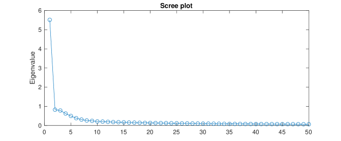
To employ the proposed estimation procedure and other comparison methods, we need to choose the rank $r_{1}$ and $r_{2}$. We first calculated 503 daily integrated volatility matrices using the PRVM estimation method in (4.1). Then, we estimated the rank $r_{1}$ using the procedure suggested by Ait-Sahalia and Xiu (2017) as follows:

$$\widehat{r}_{1}=\arg\min_{1\leq j\leq r_{\max}}\sum_{d=1}^{503}\left[p^{-1}\widehat{\xi}_{d,j}+j\times c_{1}\left\{\sqrt{\frac{\log p}{m^{1/2}}+p^{-1}\log p}\right\}^{c_{2}}\right]-1,$$ (5.1)

where $\widehat{\xi}_{d,j}$ is the $j$-th largest eigenvalue of PRVM estimator, $r_{\max}=20$, $c_{1}=0.15\times\widehat{\xi}_{d,20}$, and $c_{2}=0.5$. The above method suggests $\widehat{r}_{1}=3$. In addition, Figure 2 represents the scree plot using the first 50 eigenvalues of the sum of 503 PRVM estimates. Figure 2 confirms that this choice is reasonable. To estimate the rank $r_{2}$, we employed the largest singular value gap method as discussed in Section 2.3. From those results, we set $r_{1}=3$ and $r_{2}=1$ for the empirical study.

To predict the conditional expected volatility matrix $E(\bm{\Gamma}_{D+1}|{\cal I}_{D})$, we employed the PT-POET, POET, FIVAR, and T-POET methods as described in Section 4. Additionally, for robustness checks, we included PT-POET2, which is based on $r_{1}=3$ and $r_{2}=2$. We also considered FIVAR-H, which incorporates a HAR structure to predict one-day-ahead leading eigenvalues instead of using a VAR structure. For PT-POETs, we utilized the ex-post daily, weakly, and monthly realized volatility based on the first eigenvalues as covariates for $\mathbf{X}$ and used the additive polynomial basis and $J=2$. We used the rolling window scheme, where the in-sample period was one of 63, 126, or 252 days. We presented the best-performing results for FIVAR, T-POET, and PT-POETs across the range of in-sample periods. Specifically, the FIVAR method, utilizing observations from the past 252 days observations to estimate the model parameters and the previous 21 days to estimate the eigenvectors, performed best. Following Shin et al. (2021), the AR lag $h=1$ was chosen based on the Bayesian information criterion (BIC). For PT-POET and T-POET, an in-sample period of 63 days yielded the best performance. We used three different out-of-sample periods: from 2019:1 to 2019:6 (period 1), from 2019:7 to 2019:12 (period 2), from 2019:1 to 2019:12 (period 3).

Refer to caption
Figure 2: The scree plot of the first 50 eigenvalues of the sum of 503 PRVM estimates.

For all estimators except PRVM, we estimated the idiosyncratic volatility matrix using the hard thresholding scheme based on the 11 Global Industrial Classification Standard (GICS) sectors (Ait-Sahalia and Xiu, 2017; Fan et al., 2016a). Specifically, we set the idiosyncratic components to zero across different sectors while retaining them within the same sector.

Table 1: MSPEs and QLIKEs for the PRVM, POET, FIVAR, FIVAR-H, T-POET, and PT-POETs.
PRVM POET FIVAR FIVAR-H T-POET PT-POET PT-POET2
MSPE$\times 10^{4}$
Period 1 1.300 1.269 0.942 0.971 0.951 0.878 0.880
Period 2 3.184 3.163 2.035 2.047 2.704 2.025 2.039
Period 3 2.242 2.216 1.488 1.509 1.827 1.452 1.459
QLIKE$\times 10^{-3}$
Period 1 0.535 -0.030 -0.031 8.343 -0.050 -0.044
Period 2 0.574 -0.024 -0.024 10.184 -0.041 -0.041
Period 3 0.554 -0.027 -0.027 9.264 -0.046 -0.043

To measure the performance of the predicted volatility matrix, we first utilized the mean squared prediction error (MSPE) and QLIKE (Patton, 2011):

$\displaystyle\text{MSPE}=\frac{1}{T}\sum_{d=1}^{T}\|\widetilde{\bm{\Gamma}}_{d}-\widehat{\bm{\Gamma}}_{d}^{\text{POET}}\|_{F}^{2},$
$\displaystyle\text{QLIKE}=\frac{1}{T}\sum_{d=1}^{T}\log\left(\mathrm{det}\left(\widetilde{\bm{\Gamma}}_{d}\right)\right)+\text{tr}\left(\widetilde{\bm{\Gamma}}_{d}^{-1}\widehat{\bm{\Gamma}}_{d}^{\text{POET}}\right),$

where $T$ is the number of days in the out-of-sample period, $\widehat{\bm{\Gamma}}_{d}^{\text{POET}}$ is the POET estimator for the $d$-th day, which is a proxy of true volatility matrix, and $\widetilde{\bm{\Gamma}}_{d}$ is one of the one-day-ahead volatility matrix estimates from PRVM, POET, FIVAR, FIVAR-H, T-POET, PT-POET, and PT-POET2 for the $d$-th day of the out-of-sample period. In addition, since the true conditional expected large volatility matrix is unknown, we conducted the Diebold and Mariano (DM) test (Diebold and Mariano, 2002) using MSPE and QLIKE to assess the significance of differences in predictive performance. We compared the proposed PT-POET method with other methods. Table 1 reports the results of MSPEs and QLIKEs, and Table 2 shows the $p$-values for the DM tests. We note that the QLIKE results for the PRVM estimator are omitted, as its determinant is close to zero. The results indicate that the PT-POET estimators demonstrate the best overall performance, and PT-POET and PT-POET2 show statistically similar performances. This may be because incorporating the tensor structure and projection method, along with additional covariates such as ex-post realized volatility information, enhances prediction accuracy. We note that PT-POET does not statistically outperform FIVAR-H based on the DM test using MSPE. This outcome is due to the higher variance of prediction errors with FIVAR-H compared to FIVAR and PT-POET. That is, FIVAR-H is relatively volatile. To further evaluate the performance of the proposed method, we implemented the minimum variance portfolio allocation as described below.

Table 2: The $p$-values for the DM test statistic based on MSPE and QLIKE for the PRVM, POET, FIVAR, FIVAR-H, T-POET, and PT-POET2 with respect to the PT-POET.
PRVM POET FIVAR FIVAR-H T-POET PT-POET2
MSPE
Period 1 0.000*** 0.000*** 0.035** 0.242 0.012** 0.845
Period 2 0.004*** 0.005*** 0.902 0.810 0.044** 0.265
Period 3 0.001*** 0.001*** 0.062* 0.372 0.043** 0.284
QLIKE
Period 1 0.000*** 0.000*** 0.000*** 0.000*** 0.124
Period 2 0.000*** 0.005*** 0.005*** 0.000*** 0.102
Period 3 0.000*** 0.000*** 0.000** 0.000*** 0.190

Note: ***, **, and * indicate rejection of the null hypothesis at significance levels of 1%, 5%, and 10%, respectively.

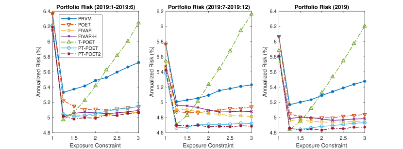
To analyze the out-of-sample portfolio allocation performance, we also considered the following constrained minimum variance portfolio allocation problem (Fan et al., 2012):

$$\min_{\omega}\omega^{T}\widetilde{\bm{\Gamma}}_{d}\omega,\text{ subject to }\omega^{\top}\mathbf{1}=1,\;\|\omega\|_{1}\leq c,$$

where $\mathbf{1}=(1,\dots,1)^{\top}\in\mathbb{R}^{p}$, the gross exposure constraint $c$ varies from 1 to 3, and $\widetilde{\bm{\Gamma}}_{d}$ is one of the one-day-ahead volatility matrix estimators obtained from PRVM, POET, FIVAR, FIVAR-H, T-POET, and PT-POETs. At the beginning of each trading day, we obtained optimal portfolios based on each estimator and held these portfolios for one day. To avoid the microstructural noise effect, we calculated the realized volatility using the 10-min portfolio log-returns. We then measured the out-of-sample risk by averaging the square root of the realized volatility for each out-of-sample period. Figure 3 illustrates the out-of-sample risks of the portfolios constructed by the PRVM, POET, FIVAR, FIVAR-H, T-POET, and PT-POET estimators. As shown in Figure 3, the PT-POET and PT-POET2 estimators demonstrate stable performance and consistently outperform the other estimators. Interestingly, while T-POET performs well in terms of global minimum risk, it becomes unstable as the gross exposure constraint increases. Additionally, PRVM and POET do not perform well. This may be because they cannot capture the dynamics of the volatility process. By considering the vector auto-regressive structure on eigenvalues of the volatility matrix, FIVAR shows improved performance compared to POET. However, FIVAR underperforms PT-POET because it does not consider the time-varying eigenvector. When comparing PT-POET and PT-POET2, PT-POET2 shows a more stable performance. This may be because adding an additional dimension of time series helps account for the eigenvector dynamics. Overall, these results indicate that the PT-POET method can efficiently predict the large integrated volatility matrix by incorporating interday time series dynamics based on both time-varying eigenvector and eigenvalue structures.

Refer to caption
Figure 3: The out-of-sample risks of the minimum variance portfolios constructed by the PRVM, POET, FIVAR, FIVAR-H, T-POET, PT-POET estimators.

6 Conclusion

This paper introduces a novel procedure for predicting large integrated volatility matrices using high-frequency financial data. The proposed PT-POET method leverages daily volatility dynamics based on the semiparametric structure of the low-rank tensor component of the integrated volatility matrix process. We establish the asymptotic properties of PT-POET and its estimator for the future integrated volatility matrix.

In the empirical study, PT-POET outperforms conventional methods in terms of out-of-sample performance for predicting the one-day-ahead integrated volatility matrix and portfolio allocation. This finding confirms that generalizing the low-rank structure and incorporating the HAR model structure into interday volatility dynamics improves the prediction of future volatility matrices. We note that, in this paper, we developed a generalized model for large volatility matrix processes and utilized the past leading eigenvalues as covariates for projecting the dynamics of singular vectors. However, it would be an interesting direction for future research to explore other possible covariates, such as trading volume, with alternative basis functions. This study requires extensive empirical research. Thus, we leave this for future research.

References

  • Ahn and Horenstein (2013) Ahn, S. C. and A. R. Horenstein (2013): “Eigenvalue ratio test for the number of factors,” Econometrica, 81, 1203–1227.
  • Aït-Sahalia et al. (2010) Aït-Sahalia, Y., J. Fan, and D. Xiu (2010): “High-frequency covariance estimates with noisy and asynchronous financial data,” Journal of the American Statistical Association, 105, 1504–1517.
  • Aït-Sahalia and Xiu (2016) Aït-Sahalia, Y. and D. Xiu (2016): “Increased correlation among asset classes: Are volatility or jumps to blame, or both?” Journal of Econometrics, 194, 205–219.
  • Ait-Sahalia and Xiu (2017) Ait-Sahalia, Y. and D. Xiu (2017): “Using principal component analysis to estimate a high dimensional factor model with high-frequency data,” Journal of Econometrics, 201, 384–399.
  • Andersen et al. (2003) Andersen, T. G., T. Bollerslev, F. X. Diebold, and P. Labys (2003): “Modeling and forecasting realized volatility,” Econometrica, 71, 579–625.
  • Bai (2003) Bai, J. (2003): “Inferential theory for factor models of large dimensions,” Econometrica, 71, 135–171.
  • Bai and Ng (2002) Bai, J. and S. Ng (2002): “Determining the number of factors in approximate factor models,” Econometrica, 70, 191–221.
  • Barndorff-Nielsen et al. (2008) Barndorff-Nielsen, O. E., P. R. Hansen, A. Lunde, and N. Shephard (2008): “Designing realized kernels to measure the ex post variation of equity prices in the presence of noise,” Econometrica, 76, 1481–1536.
  • Barndorff-Nielsen et al. (2011a) ——— (2011a): “Multivariate realised kernels: consistent positive semi-definite estimators of the covariation of equity prices with noise and non-synchronous trading,” Journal of Econometrics, 162, 149–169.
  • Barndorff-Nielsen et al. (2011b) ——— (2011b): “Subsampling realised kernels,” Journal of Econometrics, 160, 204–219.
  • Bibinger et al. (2014) Bibinger, M., N. Hautsch, P. Malec, and M. Reiß (2014): “Estimating the quadratic covariation matrix from noisy observations: Local method of moments and efficiency,” The Annals of Statistics, 42, 1312–1346.
  • Bibinger and Winkelmann (2015) Bibinger, M. and L. Winkelmann (2015): “Econometrics of co-jumps in high-frequency data with noise,” Journal of Econometrics, 184, 361–378.
  • Cai and Liu (2011) Cai, T. and W. Liu (2011): “Adaptive thresholding for sparse covariance matrix estimation,” Journal of the American Statistical Association, 106, 672–684.
  • Candes and Plan (2010) Candes, E. J. and Y. Plan (2010): “Matrix completion with noise,” Proceedings of the IEEE, 98, 925–936.
  • Chen and Fan (2023) Chen, E. Y. and J. Fan (2023): “Statistical inference for high-dimensional matrix-variate factor models,” Journal of the American Statistical Association, 118, 1038–1055.
  • Chen et al. (2024) Chen, E. Y., D. Xia, C. Cai, and J. Fan (2024): “Semi-parametric tensor factor analysis by iteratively projected singular value decomposition,” Journal of the Royal Statistical Society Series B: Statistical Methodology, 86, 793–823.
  • Chen (2007) Chen, X. (2007): “Large sample sieve estimation of semi-nonparametric models,” Handbook of Econometrics, 6, 5549–5632.
  • Cho et al. (2017) Cho, J., D. Kim, and K. Rohe (2017): “Asymptotic theory for estimating the singular vectors and values of a partially-observed low rank matrix with noise,” Statistica Sinica, 1921–1948.
  • Christensen et al. (2010) Christensen, K., S. Kinnebrock, and M. Podolskij (2010): “Pre-averaging estimators of the ex-post covariance matrix in noisy diffusion models with non-synchronous data,” Journal of Econometrics, 159, 116–133.
  • Corsi (2009) Corsi, F. (2009): “A simple approximate long-memory model of realized volatility,” Journal of Financial Econometrics, 7, 174–196.
  • De Lathauwer et al. (2000) De Lathauwer, L., B. De Moor, and J. Vandewalle (2000): “A multilinear singular value decomposition,” SIAM journal on Matrix Analysis and Applications, 21, 1253–1278.
  • Diebold and Mariano (2002) Diebold, F. X. and R. S. Mariano (2002): “Comparing predictive accuracy,” Journal of Business & Economic Statistics, 20, 134–144.
  • Fan et al. (2008) Fan, J., Y. Fan, and J. Lv (2008): “High dimensional covariance matrix estimation using a factor model,” Journal of Econometrics, 147, 186–197.
  • Fan et al. (2016a) Fan, J., A. Furger, and D. Xiu (2016a): “Incorporating global industrial classification standard into portfolio allocation: A simple factor-based large covariance matrix estimator with high-frequency data,” Journal of Business & Economic Statistics, 34, 489–503.
  • Fan and Kim (2018) Fan, J. and D. Kim (2018): “Robust high-dimensional volatility matrix estimation for high-frequency factor model,” Journal of the American Statistical Association, 113, 1268–1283.
  • Fan et al. (2011) Fan, J., Y. Liao, and M. Mincheva (2011): “High dimensional covariance matrix estimation in approximate factor models,” The Annals of Statistics, 39, 3320.
  • Fan et al. (2013) ——— (2013): “Large covariance estimation by thresholding principal orthogonal complements,” Journal of the Royal Statistical Society Series B: Statistical Methodology, 75, 603–680.
  • Fan et al. (2016b) Fan, J., Y. Liao, and W. Wang (2016b): “Projected principal component analysis in factor models,” The Annals of Statistics, 44, 219.
  • Fan et al. (2018a) Fan, J., H. Liu, and W. Wang (2018a): “Large covariance estimation through elliptical factor models,” The Annals of Statistics, 46, 1383.
  • Fan et al. (2018b) Fan, J., W. Wang, and Y. Zhong (2018b): “An $\infty$ eigenvector perturbation bound and its application to robust covariance estimation,” Journal of Machine Learning Research, 18, 1–42.
  • Fan and Wang (2007) Fan, J. and Y. Wang (2007): “Multi-scale jump and volatility analysis for high-frequency financial data,” Journal of the American Statistical Association, 102, 1349–1362.
  • Fan et al. (2012) Fan, J., J. Zhang, and K. Yu (2012): “Vast portfolio selection with gross-exposure constraints,” Journal of the American Statistical Association, 107, 592–606.
  • Hansen et al. (2012) Hansen, P. R., Z. Huang, and H. H. Shek (2012): “Realized GARCH: a joint model for returns and realized measures of volatility,” Journal of Applied Econometrics, 27, 877–906.
  • Jacod et al. (2009) Jacod, J., Y. Li, P. A. Mykland, M. Podolskij, and M. Vetter (2009): “Microstructure noise in the continuous case: the pre-averaging approach,” Stochastic Processes and their Applications, 119, 2249–2276.
  • Kim and Fan (2019) Kim, D. and J. Fan (2019): “Factor GARCH-Itô models for high-frequency data with application to large volatility matrix prediction,” Journal of Econometrics, 208, 395–417.
  • Kim et al. (2018) Kim, D., Y. Liu, and Y. Wang (2018): “Large volatility matrix estimation with factor-based diffusion model for high-frequency financial data,” Bernoulli, 24, 3657.
  • Kim and Wang (2016) Kim, D. and Y. Wang (2016): “Unified discrete-time and continuous-time models and statistical inferences for merged low-frequency and high-frequency financial data,” Journal of Econometrics, 194, 220–230.
  • Koike (2016) Koike, Y. (2016): “Quadratic covariation estimation of an irregularly observed semimartingale with jumps and noise,” Bernoulli, 22, 1894–1936.
  • Kolda and Bader (2009) Kolda, T. G. and B. W. Bader (2009): “Tensor decompositions and applications,” SIAM review, 51, 455–500.
  • Kong et al. (2023) Kong, X.-B., J.-G. Lin, C. Liu, and G.-Y. Liu (2023): “Discrepancy between global and local principal component analysis on large-panel high-frequency data,” Journal of the American Statistical Association, 118, 1333–1344.
  • Kong and Liu (2018) Kong, X.-B. and C. Liu (2018): “Testing against constant factor loading matrix with large panel high-frequency data,” Journal of Econometrics, 204, 301–319.
  • Lam and Yao (2012) Lam, C. and Q. Yao (2012): “Factor modeling for high-dimensional time series: inference for the number of factors,” The Annals of Statistics, 694–726.
  • Li and Linton (2022) Li, Z. M. and O. Linton (2022): “A ReMeDI for microstructure noise,” Econometrica, 90, 367–389.
  • Onatski (2010) Onatski, A. (2010): “Determining the number of factors from empirical distribution of eigenvalues,” The Review of Economics and Statistics, 92, 1004–1016.
  • Patton (2011) Patton, A. J. (2011): “Volatility forecast comparison using imperfect volatility proxies,” Journal of Econometrics, 160, 246–256.
  • Rothman et al. (2009) Rothman, A. J., E. Levina, and J. Zhu (2009): “Generalized thresholding of large covariance matrices,” Journal of the American Statistical Association, 104, 177–186.
  • Shephard and Sheppard (2010) Shephard, N. and K. Sheppard (2010): “Realising the future: forecasting with high-frequency-based volatility (HEAVY) models,” Journal of Applied Econometrics, 25, 197–231.
  • Shin et al. (2023) Shin, M., D. Kim, and J. Fan (2023): “Adaptive robust large volatility matrix estimation based on high-frequency financial data,” Journal of Econometrics, 237, 105514.
  • Shin et al. (2021) Shin, M., D. Kim, Y. Wang, and J. Fan (2021): “Factor and idiosyncratic VAR-Itô volatility models for heavy-tailed high-frequency financial data,” arXiv preprint arXiv:2109.05227.
  • Song et al. (2021) Song, X., D. Kim, H. Yuan, X. Cui, Z. Lu, Y. Zhou, and Y. Wang (2021): “Volatility analysis with realized GARCH-Itô models,” Journal of Econometrics, 222, 393–410.
  • Stock and Watson (2002) Stock, J. H. and M. W. Watson (2002): “Forecasting using principal components from a large number of predictors,” Journal of the American Statistical Association, 97, 1167–1179.
  • Su and Wang (2017) Su, L. and X. Wang (2017): “On time-varying factor models: Estimation and testing,” Journal of Econometrics, 198, 84–101.
  • Tao et al. (2013) Tao, M., Y. Wang, and X. Chen (2013): “Fast convergence rates in estimating large volatility matrices using high-frequency financial data,” Econometric Theory, 29, 838–856.
  • Xiu (2010) Xiu, D. (2010): “Quasi-maximum likelihood estimation of volatility with high frequency data,” Journal of Econometrics, 159, 235–250.
  • Zhang (2006) Zhang, L. (2006): “Efficient estimation of stochastic volatility using noisy observations: A multi-scale approach,” Bernoulli, 12, 1019–1043.
  • Zhang (2011) ——— (2011): “Estimating covariation: Epps effect, microstructure noise,” Journal of Econometrics, 160, 33–47.
  • Zhang et al. (2005) Zhang, L., P. A. Mykland, and Y. Aït-Sahalia (2005): “A tale of two time scales: Determining integrated volatility with noisy high-frequency data,” Journal of the American Statistical Association, 100, 1394–1411.

Appendix A Appendix

A.1 Related Lemmas

We first prove provide useful lemmas below. For each $l=1,\dots,D$, let $\{\delta_{l,i},\xi_{l,i}\}_{i=1}^{p}$ be the eigenvalues and their corresponding eigenvectors of $\bm{\Gamma}_{l}$ in decreasing order. Similarly, for each $l=1,\dots,D$, let $\{\widetilde{\delta}_{l,i},\widetilde{\xi}_{l,i}\}_{i=1}^{r_{1}}$ be the leading eigenvalues and eigenvectors of $\bm{\Psi}_{l}$ and the rest zero.

Under the pervasive condition, we have the following lemma using Weyl’s theorem.

Lemma A.1.

Under Assumption 3.1(i), for each $l\leq D$,

$$|\widetilde{\delta}_{l,i}-\delta_{l,i}|=\|\bm{\Sigma}_{l}\|\text{ for }i\leq r_{1},\qquad|\delta_{l,i}|\leq\|\bm{\Sigma}_{l}\|\text{ for }i>r_{1},$$

and, for $i\leq r_{1}$, $\widetilde{\delta}_{i}/p$ is strictly bigger than zero for all $p$.

In addition, under Assumption 3.1 (iv), for each $l\leq D$, we have

$$|\bar{\delta}_{l,i}-\delta_{l,i}|=O_{P}\left(pm^{-\frac{1}{4}}\sqrt{\log(pD\vee m)}\right)\text{ for }i\leq r_{1}.$$

The following lemma presents the individual convergence rate of leading eigenvectors using Lemma A.1 and the $l_{\infty}$ norm perturbation bound theorem of Fan et al. (2018b).

Lemma A.2.

Under Assumption 3.1, we have the following results:

  • (i)

    $\max_{l\leq D,i\leq r_{1}}\|\widetilde{\xi}_{l,i}-\xi_{l,i}\|_{\infty}\leq C\frac{\|\bm{\Sigma}_{l}\|_{\infty}}{p^{3/2}};$

  • (ii)

    $\max_{l\leq D,i\leq r_{1}}\|\bar{\xi}_{l,i}-\xi_{l,i}\|_{\infty}=O_{P}\left(m^{-\frac{1}{4}}\sqrt{\log(pD\vee m)/p}\right).$

Proof.

We first consider (i). For $l\leq D$ and $i\leq r_{1}$, $\widetilde{\delta}_{l,i}\asymp p$ and $\|\widetilde{\xi}_{l,i}\|_{\infty}\leq C/\sqrt{p}$ from Lemma A.1. Then, by Assumption 3.1 (i)–(ii) and Theorem 1 of Fan et al. (2018b), we have

$$\max_{l\leq D,i\leq r_{1}}\|\widetilde{\xi}_{l,i}-\xi_{l,i}\|_{\infty}\leq C\frac{\|\bm{\Sigma}_{l}\|_{\infty}}{D_{\delta}\sqrt{p}}.$$

where the eigengap $D_{\delta}=\min\{\widetilde{\delta}_{i}-\widetilde{\delta}_{i+1}:1\leq i\leq r_{1}\}$ and $\widetilde{\delta}_{r_{1}+1}=0$.

We consider (ii). By Theorem 1 of Fan et al. (2018b), Lemma A.2(i) and Assumption 3.1, we have

$\displaystyle\|\bar{\xi}_{l,i}-\xi_{l,i}\|_{\infty}$ $\displaystyle\leq C\frac{\|\widehat{\bm{\Gamma}}_{l}-\bm{\Gamma}\|_{\infty}}{p\sqrt{p}}=O_{P}\left(m^{-\frac{1}{4}}\sqrt{\log(pD\vee m)/p}\right).$

Lemma A.3.

Under Assumption 3.1, for $l\leq D$, we have

$$\|\bar{\bm{\Psi}}_{l}-\bm{\Psi}_{l}\|_{\max}=O_{P}(\varphi_{m}),$$

where $\varphi_{m}=m^{-\frac{1}{4}}\sqrt{\log(pD\vee m)}+s_{p}/p$.

Proof.

Let $\bm{\Psi}_{l}=\widetilde{\bm{\Xi}}\widetilde{\bm{\Delta}}\widetilde{\bm{\Xi}}^{\top}$, where $\widetilde{\bm{\Delta}}=\mathrm{diag}(\widetilde{\delta}_{l,1},\dots,\widetilde{\delta}_{l,r_{1}})$ and $\widetilde{\bm{\Xi}}=(\widetilde{\xi}_{l,1},\dots,\widetilde{\xi}_{l,r_{1}})$. Also, we let $\bm{\Delta}=\mathrm{diag}(\delta_{l,1},\dots,\delta_{l,r_{1}})$ and the corresponding eigenvectors $\bm{\Xi}=(\xi_{l,1},\dots,\xi_{\l,r_{1}})$ of covariance matrix $\bm{\Gamma}_{l}$. Note that $\|\widetilde{\bm{\Xi}}\widetilde{\bm{\Delta}}^{1/2}\|_{\max}=O(1)$ and $\|\bm{\Sigma}_{l}\|_{\infty}=O(s_{p})$. By Lemmas A.1A.2, we have

$\displaystyle\|\bm{\Xi}\bm{\Delta}^{\frac{1}{2}}-\widetilde{\bm{\Xi}}\widetilde{\bm{\Delta}}^{{\frac{1}{2}}}\|_{\max}$ $\displaystyle\leq\|\widetilde{\bm{\Xi}}(\bm{\Delta}^{{\frac{1}{2}}}-\widetilde{\bm{\Delta}}^{{\frac{1}{2}}})\|_{\max}+\|(\bm{\Xi}-\widetilde{\bm{\Xi}})\bm{\Delta}^{{\frac{1}{2}}}\|_{\max}$
$\displaystyle\leq C\cfrac{\|\widetilde{\bm{\Xi}}\widetilde{\bm{\Delta}}^{1/2}\|_{\max}}{\sqrt{p}}+C\cfrac{\|\bm{\Sigma}_{l}\|_{\infty}}{p}=o\left(1\right).$

Hence, we have $\|\bm{\Xi}\bm{\Delta}^{\frac{1}{2}}\|_{\max}=O(1)$ and $\|\bm{\Xi}\|_{\max}=O(1/\sqrt{p})$. Recall that $\bar{\bm{\Psi}}_{l}=\sum_{i=1}^{r_{1}}\bar{\delta}_{l,i}\bar{\xi}_{l,i}\bar{\xi}_{l,i}^{\prime}$, where $\{\bar{\delta}_{l,i},\bar{\xi}_{l,i}\}_{i=1}^{p}$ are the eigenvalues and eigenvectors of $\widehat{\bm{\Gamma}}_{l}$ in decreasing order, and we denote $\bar{\bm{\Delta}}=\mathrm{diag}(\bar{\delta}_{l,1},\dots,\bar{\delta}_{l,r_{1}})$ and $\bar{\bm{\Xi}}=(\bar{\xi}_{l,1},\dots,\bar{\xi}_{\l,r_{1}})$. By the above fact and the results from Lemmas A.1A.2, we have

$\displaystyle\|\widetilde{\bm{\Xi}}\widetilde{\bm{\Delta}}\widetilde{\bm{\Xi}}^{\prime}-\bm{\Xi}\bm{\Delta}\bm{\Xi}^{\prime}\|_{\max}\leq\|\widetilde{\bm{\Xi}}(\widetilde{\bm{\Delta}}-\bm{\Delta})\widetilde{\bm{\Xi}}^{\prime}\|_{\max}+\|(\widetilde{\bm{\Xi}}-\bm{\Xi})\bm{\Delta}(\widetilde{\bm{\Xi}}-\bm{\Xi})^{\prime}\|_{\max}+2\|\bm{\Xi}\bm{\Delta}(\widetilde{\bm{\Xi}}-\bm{\Xi})^{\prime}\|_{\max}$
$\displaystyle\;\;\;\;\;=O(p^{-1}\|\widetilde{\bm{\Delta}}-\bm{\Delta}\|_{\max}+\sqrt{p}\|\widetilde{\bm{\Xi}}-\bm{\Xi}\|_{\max})=O(s_{p}/p),$
$\displaystyle\|\bar{\bm{\Xi}}\bar{\bm{\Delta}}\bar{\bm{\Xi}}^{\prime}-\bm{\Xi}\bm{\Delta}\bm{\Xi}^{\prime}\|_{\max}\leq\|\bar{\bm{\Xi}}(\bar{\bm{\Delta}}-\bm{\Delta})\bar{\bm{\Xi}}^{\prime}\|_{\max}+\|(\bar{\bm{\Xi}}-\bm{\Xi})\bm{\Delta}(\bar{\bm{\Xi}}-\bm{\Xi})^{\prime}\|_{\max}+2\|\bm{\Xi}\bm{\Delta}(\bar{\bm{\Xi}}-\bm{\Xi})^{\prime}\|_{\max}$
$\displaystyle\;\;\;\;\;=O_{P}(p^{-1}\|\bar{\bm{\Delta}}-\bm{\Delta}\|_{\max}+\sqrt{p}\|\bar{\bm{\Xi}}-\bm{\Xi}\|_{\max})=O_{P}\left(m^{-\frac{1}{4}}\sqrt{\log(pD\vee m)}\right).$

Thus, we have

$$\|\bar{\bm{\Psi}}_{l}-\bm{\Psi}_{l}\|_{\max}=\|\bar{\bm{\Xi}}\bar{\bm{\Delta}}\bar{\bm{\Xi}}^{\prime}-\widetilde{\bm{\Xi}}\widetilde{\bm{\Delta}}\widetilde{\bm{\Xi}}^{\prime}\|_{\max}=O_{P}\left(m^{-\frac{1}{4}}\sqrt{\log(pD\vee m)}+s_{p}/p\right).$$ (A.1)

The following lemma presents the individual convergence rate of leading left singular vector estimators.

Lemma A.4.

Under Assumptions 3.13.3, we have the following results:

(i) $\displaystyle\|\widehat{\mathbf{Q}}-\mathbf{Q}\|_{\max}=O_{P}\left(\frac{m^{-\frac{1}{4}}\sqrt{J\log(pD\vee m)}}{\sqrt{p}}+\frac{s_{p}J^{\frac{1}{2}}}{p^{\frac{3}{2}}}+\frac{J^{\frac{1-\kappa}{2}}}{\sqrt{p}}\right);$
(ii) $\displaystyle\|\widehat{\mathbf{G}}(\mathbf{X})-\mathbf{G}(\mathbf{X})\|_{\max}=O_{P}\left(\frac{m^{-\frac{1}{4}}\sqrt{J\log(pD\vee m)}}{\sqrt{D}}+\frac{s_{p}J^{\frac{1}{2}}}{p\sqrt{D}}+\frac{J^{\frac{1-\kappa}{2}}}{\sqrt{D}}\right).$
Proof.

We first consider (i). Let the singular value decomposition be ${\cal M}_{1}({\cal S})=\mathbf{Q}\bm{\Lambda}\mathbf{H}^{\top}$, where the $p\times r_{1}$ matrix $\mathbf{Q}=(\mathbf{q}_{1},\dots,\mathbf{q}_{r_{1}})$ and the $pD\times r_{1}$ matrix $\mathbf{H}=(\mathbf{h}_{1},\dots,\mathbf{h}_{r_{1}})$ consist of the singular vectors. We denote the eigengap $\bar{\gamma}_{1}=\min\{\sigma_{k}({\cal M}_{1}({\cal S}))-\sigma_{k+1}({\cal M}_{1}({\cal S})):1\leq k\leq r_{1}\}$ and $\sigma_{r_{1}+1}({\cal M}_{1}({\cal S}))=0$. For $k\leq r_{1}$, $\sigma_{k}({\cal M}_{1}({\cal S}))\asymp p\sqrt{D}$ and $\|\mathbf{q}_{k}\|_{\infty}\leq C/\sqrt{p}$ and $\|\mathbf{h}_{k}\|_{\infty}\leq C/\sqrt{pD}$. In addition, the coherences $\mu(\mathbf{Q})=p\max_{i}\sum_{k=1}^{r_{1}}q_{i,k}^{2}/r_{1}\leq C$ and $\mu(\mathbf{H})=pD\max_{i}\sum_{k=1}^{r_{1}}h_{i,k}^{2}/r_{1}\leq C$, where $q_{i,k}$ and $h_{i,k}$ are the $(i,k)$ entry of $\mathbf{Q}$ and $\mathbf{H}$, respectively. Let $\widehat{\mathbf{Q}}=(\widehat{\mathbf{q}}_{1},\dots,\widehat{\mathbf{q}}_{r_{1}})$. Then, by Theorem 1 of Fan et al. (2018b), we have

$\displaystyle\max_{k\leq r_{1}}\|\widehat{\mathbf{q}}_{k}-\mathbf{q}_{k}\|_{\infty}$
$\displaystyle\leq C\frac{\max\{\sqrt{D}\|{\cal M}_{1}(\widetilde{{\cal S}})-{\cal M}_{1}({\cal S})\|_{1},\frac{1}{\sqrt{D}}\|{\cal M}_{1}(\widetilde{{\cal S}})-{\cal M}_{1}({\cal S})\|_{\infty}\}}{\bar{\gamma}_{1}\sqrt{p}}$
$\displaystyle\leq C\frac{p\sqrt{D}\left(\|{\cal M}_{1}(\widetilde{{\cal S}})-{\cal M}_{1}({\cal S}\times_{3}\mathbf{P})\|_{\max}+\|{\cal M}_{1}({\cal S}\times_{3}\mathbf{P})-{\cal M}_{1}({\cal S})\|_{\max}\right)}{\bar{\gamma}_{1}\sqrt{p}}$
$\displaystyle=O_{P}\left(\frac{m^{-\frac{1}{4}}\sqrt{J\log(pD\vee m)}}{\sqrt{p}}+\frac{s_{p}J^{\frac{1}{2}}}{p^{\frac{3}{2}}}+\frac{J^{\frac{1-\kappa}{2}}}{\sqrt{p}}\right),$

where the last line is due to Lemma A.6 below.

We consider (ii). Similar to part (i), by Lemma A.6 and Theorem 1 of Fan et al. (2018b), we have

$\displaystyle\max_{k\leq r_{2}}\|\widehat{\mathbf{v}}_{k}-\mathbf{v}_{k}\|_{\infty}$
$\displaystyle\leq C\frac{\max\{\frac{p}{\sqrt{D}}\|{\cal M}_{3}(\widetilde{{\cal S}})-{\cal M}_{3}({\cal S})\|_{1},\frac{\sqrt{D}}{p}\|{\cal M}_{3}(\widetilde{{\cal S}})-{\cal M}_{3}({\cal S})\|_{\infty}\}}{\bar{\gamma}\sqrt{D}}$
$\displaystyle\leq C\frac{p\sqrt{D}\left(\|{\cal M}_{3}(\widetilde{{\cal S}})-{\cal M}_{3}({\cal S}\times_{3}\mathbf{P})\|_{\max}+\|{\cal M}_{3}({\cal S}\times_{3}\mathbf{P})-{\cal M}_{3}({\cal S})\|_{\max}\right)}{\bar{\gamma}\sqrt{D}}$
$\displaystyle=O_{P}\left(\frac{m^{-\frac{1}{4}}\sqrt{J\log(pD\vee m)}}{\sqrt{D}}+\frac{s_{p}J^{\frac{1}{2}}}{p\sqrt{D}}+\frac{J^{\frac{1-\kappa}{2}}}{\sqrt{D}}\right).$

Lemma A.5.

Under Assumptions 3.13.3, we have

$\displaystyle\|{\cal M}_{1}(\widehat{{\cal F}})-{\cal M}_{1}({\cal F})\|_{\max}=O_{P}\left(p\sqrt{D}m^{-\frac{1}{4}}\sqrt{J\log(pD\vee m)}+s_{p}\sqrt{JD}+p\sqrt{D}J^{\frac{1-\kappa}{2}}\right).$
Proof.

By Lemma A.6, we have

$\displaystyle\|{\cal M}_{1}(\widetilde{{\cal S}})-{\cal M}_{1}({\cal S})\|$ $\displaystyle\leq\|{\cal M}_{1}(\mathbf{P}\bar{{\cal S}})-{\cal M}_{1}(\mathbf{P}{\cal S})\|+\|{\cal M}_{1}(\mathbf{P}{\cal S})-{\cal M}_{1}({\cal S})\|$
$\displaystyle=O_{P}\left(p\sqrt{D}m^{-\frac{1}{4}}\sqrt{J\log(pD\vee m)}+s_{p}\sqrt{JD}+p\sqrt{D}J^{\frac{1-\kappa}{2}}\right).$

We denote $\widehat{\mathbf{V}}=\widehat{\mathbf{G}}(\mathbf{X})$. By Lemma A.4, we have $\|\widehat{\mathbf{V}}\otimes\widehat{\mathbf{Q}}-\mathbf{V}\otimes\mathbf{Q}\|\leq\sqrt{pD}\|\widehat{\mathbf{V}}\otimes\widehat{\mathbf{Q}}-\mathbf{V}\otimes\mathbf{Q}\|_{\max}\leq O(\sqrt{p}\|\widehat{\mathbf{Q}}-\mathbf{Q}\|_{\max}+\sqrt{D}\|\widehat{\mathbf{V}}-\mathbf{V}\|_{\max})=O_{P}(m^{-\frac{1}{4}}\sqrt{J\log(pD\vee m)}+s_{p}J^{\frac{1}{2}}/p+J^{\frac{1-\kappa}{2}})$. Note that $\|{\cal M}_{1}({\cal S})\|=O(p\sqrt{D})$, $\|\mathbf{Q}\|_{\max}=O(1/\sqrt{p})$ and $\|\mathbf{V}\otimes\mathbf{Q}\|_{\max}=O(1/\sqrt{pD})$. By using the above results, we can obtain

$\displaystyle\|{\cal M}_{1}(\widehat{{\cal F}})-{\cal M}_{1}({\cal F})\|_{\max}\leq\|\widehat{\mathbf{Q}}^{\top}{\cal M}_{1}(\widetilde{{\cal S}})(\widehat{\mathbf{V}}\otimes\widehat{\mathbf{Q}})-\mathbf{Q}^{\top}{\cal M}_{1}({\cal S})(\mathbf{V}\otimes\mathbf{Q})\|$
$\displaystyle\quad\leq\|\widehat{\mathbf{Q}}^{\top}({\cal M}_{1}(\widetilde{{\cal S}})-{\cal M}_{1}({\cal S}))(\widehat{\mathbf{V}}\otimes\widehat{\mathbf{Q}})\|+\|(\widehat{\mathbf{Q}}-\mathbf{Q})^{\top}{\cal M}_{1}({\cal S})(\widehat{\mathbf{V}}\otimes\widehat{\mathbf{Q}}-\mathbf{V}\otimes\mathbf{Q})\|$
$\displaystyle\quad+\|\mathbf{Q}^{\top}{\cal M}_{1}({\cal S})(\widehat{\mathbf{V}}\otimes\widehat{\mathbf{Q}}-\mathbf{V}\otimes\mathbf{Q})\|+\|(\widehat{\mathbf{Q}}-\mathbf{Q})^{\top}{\cal M}_{1}({\cal S})(\mathbf{V}\otimes\mathbf{Q})\|$
$\displaystyle\quad=O_{P}\left(p\sqrt{D}m^{-\frac{1}{4}}\sqrt{J\log(pD\vee m)}+s_{p}\sqrt{JD}+p\sqrt{D}J^{\frac{1-\kappa}{2}}\right).$

Lemma A.6.

Under Assumptions 3.13.3, we have

  • (i)

    $\|{\cal M}_{1}(\widetilde{{\cal S}})-{\cal M}_{1}({\cal S}\times_{3}\mathbf{P})\|_{\max}=O_{P}(m^{-1/4}\sqrt{J\log(pD\vee m)}+s_{p}\sqrt{J}/p)$;

  • (ii)

    $\|{\cal M}_{1}({\cal S}\times_{3}\mathbf{P})-{\cal M}_{1}({\cal S})\|_{\max}=O_{P}(J^{\frac{1-\kappa}{2}})$.

Proof.

We first consider (i). Let ${\cal M}_{3}(\widehat{{\cal S}})-{\cal M}_{3}({\cal S})=\mathbf{M}=(\mathbf{m}_{1},\dots,\mathbf{m}_{p^{2}})$. By Lemma A.3, $\|{\cal M}_{1}(\bar{{\cal S}})-{\cal M}_{1}({\cal S})\|_{\max}=\|{\cal M}_{3}(\bar{{\cal S}})-{\cal M}_{3}({\cal S})\|_{\max}=O_{P}(\varphi_{m})$, where $\varphi_{m}=m^{-\frac{1}{4}}\sqrt{\log(pD\vee m)}+s_{p}/p$. By Assumption 3.2, $\|(\bm{\Phi}(\mathbf{X})^{\prime}\bm{\Phi}(\mathbf{X}))^{-1}\|=\lambda_{\min}^{-1}(D^{-1}\bm{\Phi}(\mathbf{X})^{\prime}\bm{\Phi}(\mathbf{X}))D^{-1}=O_{P}(D^{-1})$, and $\|\bm{\Phi}(\mathbf{X})\|=O_{P}(D^{1/2})$. Then, we can show

$\displaystyle\|{\cal M}_{1}(\bar{{\cal S}}\times_{3}\mathbf{P})-{\cal M}_{1}({\cal S}\times_{3}\mathbf{P})\|_{\max}=\|{\cal M}_{3}(\bar{{\cal S}}\times_{3}\mathbf{P})-{\cal M}_{3}({\cal S}\times_{3}\mathbf{P})\|_{\max}$
$\displaystyle\quad=\|\mathbf{P}{\cal M}_{3}(\bar{{\cal S}})-\mathbf{P}{\cal M}_{3}({\cal S})\|_{\max}=\|\mathbf{P}({\cal M}_{3}(\bar{{\cal S}})-{\cal M}_{3}({\cal S}))\|_{\max}$
$\displaystyle\quad=\max_{i,j}|\phi(\mathbf{x}_{i})(\bm{\Phi}(\mathbf{X})^{\prime}\bm{\Phi}(\mathbf{X}))^{-1}\bm{\Phi}(\mathbf{X})^{\prime}\mathbf{m}_{j}|$
$\displaystyle\quad\leq\max_{i}\|\phi(\mathbf{x}_{i})\|_{F}\|(\bm{\Phi}(\mathbf{X})^{\prime}\bm{\Phi}(\mathbf{X}))^{-1}\|\|\bm{\Phi}(\mathbf{X})^{\prime}\|\|\mathbf{m}_{j}\|_{F}$
$\displaystyle\quad=O_{P}(\sqrt{J}\varphi_{m}).$

We consider (ii). Let $\phi(\mathbf{x}_{i})$ and $R(\mathbf{x}_{i})$ be the $i$th row of $\bm{\Phi}(\mathbf{X})$ and $\mathbf{R}(\mathbf{X})$, respectively. Let $\mathbf{w}_{j}$ be the $j$th row of $p^{2}\times r_{1}^{2}$ matrix $\mathbf{Q}\otimes\mathbf{Q}=\mathbf{W}$. By Assumptions 3.2 and 3.3, we have $\|\phi(\mathbf{x}_{i})\mathbf{B}\|_{F}=O_{P}(1/\sqrt{D})$ and $\|R(\mathbf{x}_{i})\|_{F}=O_{P}(J_{1}^{-\kappa/2}/\sqrt{D})$, for each $i\leq D$. Also, by Assumption 3.3 (ii), we have $\|\mathbf{R}(\mathbf{X})\|_{F}=O_{P}(J_{1}^{-\kappa/2})$. Then, we can obtain

$\displaystyle\|\mathbf{P}\mathbf{R}(\mathbf{X}){\cal M}_{3}({\cal F})(\mathbf{Q}\otimes\mathbf{Q})^{\top}\|_{\max}=\max_{i\leq D,j\leq p^{2}}|\phi(\mathbf{x}_{i})(\bm{\Phi}(\mathbf{X})^{\prime}\bm{\Phi}(\mathbf{X}))^{-1}\bm{\Phi}(\mathbf{X})^{\prime}\mathbf{R}(\mathbf{X}){\cal M}_{3}({\cal F})\mathbf{w}_{j}^{\prime}|$
$\displaystyle\qquad\qquad\qquad\leq\max_{i}\|\phi(\mathbf{x}_{i})\|_{F}\|(\bm{\Phi}(\mathbf{X})^{\prime}\bm{\Phi}(\mathbf{X}))^{-1}\|\|\bm{\Phi}(\mathbf{X})\|\|\mathbf{R}(\mathbf{X})\|_{F}\|{\cal M}_{3}({\cal F})\|\max_{j}\|\mathbf{w}_{j}^{\prime}\|_{F}$
$\displaystyle\qquad\qquad\qquad=O_{P}(J^{(1-\kappa)/2}),$

and

$\displaystyle\|\mathbf{R}(\mathbf{X}){\cal M}_{3}({\cal F})(\mathbf{Q}\otimes\mathbf{Q})^{\top}\|_{\max}$ $\displaystyle=\max_{i\leq D,j\leq p^{2}}|R(\mathbf{x}_{i}){\cal M}_{3}({\cal F})\mathbf{w}_{j}^{\prime}|$
$\displaystyle\leq\max_{i}\|R(\mathbf{x}_{i})\|_{F}\|{\cal M}_{3}({\cal F})\|\max_{j}\|\mathbf{w}_{j}^{\prime}\|_{F}=O_{P}(J^{-\kappa/2}).$

By using the above results, we can obtain

$\displaystyle\|{\cal M}_{1}({\cal S}\times_{3}\mathbf{P})-{\cal M}_{1}({\cal S})\|_{\max}=\|{\cal M}_{3}({\cal S}\times_{3}\mathbf{P})-{\cal M}_{3}({\cal S})\|_{\max}=\|\mathbf{P}{\cal M}_{3}({\cal S})-{\cal M}_{3}({\cal S})\|_{\max}$
$\displaystyle\qquad\qquad\leq\|\mathbf{P}\mathbf{R}(\mathbf{X}){\cal M}_{3}({\cal F})(\mathbf{Q}\otimes\mathbf{Q})^{\top}\|_{\max}+\|\mathbf{R}(\mathbf{X}){\cal M}_{3}({\cal F})(\mathbf{Q}\otimes\mathbf{Q})^{\top}\|_{\max}$
$\displaystyle\qquad\qquad=O_{P}(J^{(1-\kappa)/2}).$

A.2 Proof of Proposition 3.1

Proof of Proposition 3.1. We consider (3.1). By Lemma A.4, we have $\|\widehat{\mathbf{v}}_{l}\otimes\widehat{\mathbf{Q}}-\mathbf{v}_{l}\otimes\mathbf{Q}\|_{\max}\leq O(\frac{1}{\sqrt{D}}\|\widehat{\mathbf{Q}}-\mathbf{Q}\|_{\max}+\frac{1}{\sqrt{p}}\|\widehat{\mathbf{V}}-\mathbf{V}\|_{\max})=O_{P}(m^{-\frac{1}{4}}\sqrt{J\log(pD\vee m)/pD}+s_{p}J^{\frac{1}{2}}/p\sqrt{pD}+J^{\frac{1-\kappa}{2}}/\sqrt{pD}$. By Lemmas A.4A.5 and the above result, for each $l=1,\dots,D$, we have

$\displaystyle\|\widehat{\bm{\Psi}}_{l}-\bm{\Psi}_{l}\|_{\max}=\|\widehat{\mathbf{Q}}{\cal M}_{1}(\widehat{{\cal F}})(\widehat{\mathbf{v}}_{l}\otimes\widehat{\mathbf{Q}})^{\top}-\mathbf{Q}{\cal M}_{1}({\cal F})(\mathbf{v}_{l}\otimes\mathbf{Q})^{\top}\|_{\max}$
$\displaystyle\qquad\leq\|\widehat{\mathbf{Q}}({\cal M}_{1}(\widehat{{\cal F}})-{\cal M}_{1}({\cal F}))(\widehat{\mathbf{v}}_{l}\otimes\widehat{\mathbf{Q}})^{\top}\|_{\max}+\|(\widehat{\mathbf{Q}}-\mathbf{Q}){\cal M}_{1}({\cal F})(\widehat{\mathbf{v}}_{l}\otimes\widehat{\mathbf{Q}}-\mathbf{v}_{l}\otimes\mathbf{Q})^{\top}\|_{\max}$
$\displaystyle\qquad\qquad+\|\mathbf{Q}{\cal M}_{1}({\cal F})(\widehat{\mathbf{v}}_{l}\otimes\widehat{\mathbf{Q}}-\mathbf{v}_{l}\otimes\mathbf{Q})^{\top}\|_{\max}+\|(\widehat{\mathbf{Q}}-\mathbf{Q}){\cal M}_{1}({\cal F})(\mathbf{v}_{l}\otimes\mathbf{Q})^{\top}\|_{\max}$
$\displaystyle\qquad=O(\frac{1}{p\sqrt{D}}\|{\cal M}_{1}(\widehat{{\cal F}})-{\cal M}_{1}({\cal F})\|_{\max}+\sqrt{pD}\|\widehat{\mathbf{v}}_{l}\otimes\widehat{\mathbf{Q}}-\mathbf{v}_{l}\otimes\mathbf{Q}\|_{\max}+\sqrt{p}\|\widehat{\mathbf{Q}}-\mathbf{Q}\|_{\max})$
$\displaystyle\qquad=O_{P}\left(m^{-\frac{1}{4}}\sqrt{J\log(pD\vee m)}+\frac{s_{p}\sqrt{J}}{p}+J^{\frac{1-\kappa}{2}}\right).$

We consider (3.2). By the result (3.1) and Assumption 3.1(v), we have

$\displaystyle\|\widetilde{\bm{\Sigma}}_{l}-\bm{\Sigma}_{l}\|_{\max}$ $\displaystyle\leq\|\widehat{\bm{\Gamma}}_{l}-\bm{\Gamma}_{l}\|_{\max}+\|\widehat{\bm{\Psi}}_{l}-\bm{\Psi}_{l}\|_{\max}$
$\displaystyle=O_{P}\left(m^{-\frac{1}{4}}\sqrt{J\log(pD\vee m)}+\frac{s_{p}\sqrt{J}}{p}+J^{\frac{1-\kappa}{2}}\right).$

Then, $\|\widehat{\bm{\Sigma}}_{l}-\bm{\Sigma}_{l}\|_{\max}=O_{P}(\tau+\omega_{m})=O_{P}(\omega_{m})$, when $\tau$ is chosen as the same order of $\omega_{m}=m^{-\frac{1}{4}}\sqrt{J\log(pD\vee m)}+s_{p}\sqrt{J}/p+J^{\frac{1-\kappa}{2}}$. Therefore, similar to the proofs of Theorem 2.1 in Fan et al. (2011), we can show $\|\widehat{\bm{\Sigma}}_{l}-\bm{\Sigma}_{l}\|=O_{P}(s_{p}\omega_{m}^{1-\eta})$.

A.3 Proof of Theorem 3.1

Proof of Theorem 3.1. We first consider (3.3). Recall that $\widehat{\mathbf{A}}=(\bm{\Phi}(\mathbf{X})^{\prime}\bm{\Phi}(\mathbf{X}))^{-1}\bm{\Phi}(\mathbf{X})^{\prime}\widehat{\mathbf{G}}(\mathbf{X})=(\widehat{\mathbf{a}}_{1},\dots,\widehat{\mathbf{a}}_{r_{2}})$ and $\widehat{g}_{k}(\mathbf{x})=\phi(\mathbf{x})^{\prime}\widehat{\mathbf{a}}_{k}$ for $k=1,\dots,r_{2}$. Note that $\|(\bm{\Phi}(\mathbf{X})^{\prime}\bm{\Phi}(\mathbf{X}))^{-1}\|=O_{P}(D^{-1})$ and $\|\mathbf{R}(\mathbf{X})\|_{F}=O_{P}(J^{-\kappa/2})$. By Lemma A.4, we can obtain

$\displaystyle\|\widehat{\mathbf{A}}-\mathbf{A}\|_{F}^{2}$
$\displaystyle\leq\|(\bm{\Phi}(\mathbf{X})^{\prime}\bm{\Phi}(\mathbf{X}))^{-1}\bm{\Phi}(\mathbf{X})^{\prime}(\widehat{\mathbf{G}}(\mathbf{X})-\mathbf{G}(\mathbf{X}))\|_{F}^{2}+\|(\bm{\Phi}(\mathbf{X})^{\prime}\bm{\Phi}(\mathbf{X}))^{-1}\bm{\Phi}(\mathbf{X})^{\prime}\mathbf{R}(\mathbf{X})\|_{F}^{2}$
$\displaystyle\leq\|(\bm{\Phi}(\mathbf{X})^{\prime}\bm{\Phi}(\mathbf{X}))^{-1}\|^{2}\|\bm{\Phi}(\mathbf{X})\|^{2}\|\widehat{\mathbf{G}}(\mathbf{X})-\mathbf{G}(\mathbf{X})\|_{F}^{2}+\|(\bm{\Phi}(\mathbf{X})^{\prime}\bm{\Phi}(\mathbf{X}))^{-1}\|^{2}\|\bm{\Phi}(\mathbf{X})\|^{2}\|\mathbf{R}(\mathbf{X})\|_{F}^{2}$
$\displaystyle=O_{P}\left(\frac{m^{-\frac{1}{2}}J\log(pD\vee m)}{D}+\frac{s_{p}^{2}J}{p^{2}D}+\frac{J^{1-\kappa}}{D}\right).$

Since $\max_{k}\|\widehat{\mathbf{a}}_{k}-\mathbf{a}_{k}\|^{2}\leq\|\widehat{\mathbf{A}}-\mathbf{A}\|_{F}^{2}$, we have

$\displaystyle\max_{k\leq r_{2}}\sup_{\mathbf{x}\in{\cal X}}|\widehat{g}_{k}(\mathbf{x})-g_{k}(\mathbf{x})|$ $\displaystyle\leq\sup_{\mathbf{x}\in{\cal X}}\|\phi(\mathbf{x})\|\max_{k\leq r}\|\widehat{\mathbf{a}}_{k}-\mathbf{a}_{k}\|+\sup_{\mathbf{x}\in{\cal X}}\left|\sum_{l=1}^{d_{1}}R_{kl}(x_{l})\right|$
$\displaystyle=O_{P}\left(\frac{m^{-\frac{1}{4}}\sqrt{J\log(pD\vee m)}}{\sqrt{D}}+\frac{s_{p}\sqrt{J}}{p\sqrt{D}}+\frac{J^{\frac{1-\kappa}{2}}}{\sqrt{D}}\right)\sup_{\mathbf{x}\in{\cal X}}\|\phi(\mathbf{x})\|.$

By using the above result and Lemmas A.4A.5, we can obtain

$\displaystyle\|\widehat{\bm{\Psi}}_{D+1}-E(\bm{\Psi}_{D+1}|{\cal I}_{D})\|_{\max}=\|\widehat{\mathbf{Q}}{\cal M}_{1}(\widehat{{\cal F}})(\widehat{\mathbf{g}}(\mathbf{x}_{D+1})\otimes\widehat{\mathbf{Q}})^{\top}-\mathbf{Q}{\cal M}_{1}({\cal F})(\mathbf{g}(\mathbf{x}_{D+1})\otimes\mathbf{Q})^{\top}\|_{\max}$
$\displaystyle\quad\leq\|\widehat{\mathbf{Q}}({\cal M}_{1}(\widehat{{\cal F}})-{\cal M}_{1}({\cal F}))(\widehat{\mathbf{g}}(\mathbf{x}_{D+1})\otimes\widehat{\mathbf{Q}})^{\top}\|_{\max}$
$\displaystyle\quad\quad+\|(\widehat{\mathbf{Q}}-\mathbf{Q}){\cal M}_{1}({\cal F})(\widehat{\mathbf{g}}(\mathbf{x}_{D+1})\otimes\widehat{\mathbf{Q}}-\mathbf{g}(\mathbf{x}_{D+1})\otimes\mathbf{Q})^{\top}\|_{\max}$
$\displaystyle\quad\quad+\|\mathbf{Q}{\cal M}_{1}({\cal F})(\widehat{\mathbf{g}}(\mathbf{x}_{D+1})\otimes\widehat{\mathbf{Q}}-\mathbf{g}(\mathbf{x}_{D+1})\otimes\mathbf{Q})^{\top}\|_{\max}+\|(\widehat{\mathbf{Q}}-\mathbf{Q}){\cal M}_{1}({\cal F})(\mathbf{g}(\mathbf{x}_{D+1})\otimes\mathbf{Q})^{\top}\|_{\max}$
$\displaystyle\quad=O\Big{(}\frac{1}{p\sqrt{D}}\|{\cal M}_{1}(\widehat{{\cal F}})-{\cal M}_{1}({\cal F})\|_{\max}+\sqrt{p}\|\widehat{\mathbf{Q}}-\mathbf{Q}\|_{\max}$
$\displaystyle\qquad\qquad\qquad\qquad\qquad+\sqrt{pD}\|\widehat{\mathbf{g}}(\mathbf{x}_{D+1})\otimes\widehat{\mathbf{Q}}-\mathbf{g}(\mathbf{x}_{D+1})\otimes\mathbf{Q}\|_{\max}\Big{)}$
$\displaystyle\quad=O_{P}\left(m^{-\frac{1}{4}}J\sqrt{\log(pD\vee m)}+\frac{s_{p}J}{p}+J^{1-\frac{\kappa}{2}}\right)\max_{j\leq J}\sup_{x}|\phi_{j}(x)|:=O_{P}(\delta_{m,p,D}).$ (A.2)

By combining (A.2) and Proposition 3.1, we can show (3.3).

Consider (3.4). Let $\{\lambda_{i},\pi_{i}\}_{i=1}^{p}$ be the eigenvalues and their corresponding eigenvectors of $\bm{\Gamma}^{*}=E(\bm{\Gamma}_{D+1}|{\cal I}_{D})$, and we denote $\bm{\Lambda}=\mathrm{diag}(\lambda_{1},\dots,\lambda_{r_{1}})$ and $\mbox{\boldmath$\Pi$}=(\pi_{1},\dots,\pi_{r_{1}})$. Let $\widetilde{\bm{\Lambda}}=\mathrm{diag}(\widetilde{\lambda}_{1},\dots,\widetilde{\lambda}_{r_{1}})$ be the leading eigenvalues of $E(\bm{\Psi}_{D+1}|{\cal I}_{D})$ and $\widetilde{\mbox{\boldmath$\Pi$}}=(\widetilde{\pi}_{1},\dots,\widetilde{\pi}_{r_{1}})$ be their corresponding eigenvectors. Similarly, let $\widehat{\bm{\Lambda}}=\mathrm{diag}(\widehat{\lambda}_{1},\dots,\widehat{\lambda}_{r_{1}})$ be the leading eigenvalues of $\widehat{\bm{\Psi}}_{D+1}$ and $\widehat{\mbox{\boldmath$\Pi$}}=(\widehat{\pi}_{1},\dots,\widehat{\pi}_{r_{1}})$ be their corresponding eigenvectors. We consider the following four useful rates of convergence. By Weyl’s theorem, (A.2), and Assumption 3.1(iv), we have

$\displaystyle\|\widehat{\bm{\Lambda}}-\bm{\Lambda}\|_{\max}$ $\displaystyle\leq\|\widehat{\bm{\Psi}}_{D+1}-\bm{\Gamma}^{*}\|\leq\|\widehat{\bm{\Psi}}_{D+1}-E(\bm{\Psi}_{D+1}|{\cal I}_{D})\|+\|E(\bm{\Psi}_{D+1}|{\cal I}_{D})-\bm{\Gamma}^{*}\|$
$\displaystyle\leq\|\widehat{\bm{\Psi}}_{D+1}-E(\bm{\Psi}_{D+1}|{\cal I}_{D})\|_{F}+\|E(\bm{\Sigma}_{D+1}|{\cal I}_{D})\|=O_{P}(p\delta_{m,p,D}+s_{p}),$ (A.3)

and

$\displaystyle\|\widetilde{\bm{\Lambda}}-\bm{\Lambda}\|_{\max}\leq\|E(\bm{\Sigma}_{D+1}|{\cal I}_{D})\|=O_{P}(s_{p}).$ (A.4)

In addition, using the similar proof of Lemma A.2, we can obtain

$\displaystyle\max_{i\leq r_{1}}\|\widehat{\pi}_{i}-\pi_{i}\|_{\infty}$ $\displaystyle\leq C\frac{\|\widehat{\bm{\Psi}}_{D+1}-\bm{\Gamma}^{*}\|_{\infty}}{p\sqrt{p}}\leq C\frac{\|\widehat{\bm{\Psi}}_{D+1}-E(\bm{\Psi}_{D+1}|{\cal I}_{D})\|_{\infty}}{p\sqrt{p}}+C\frac{\|E(\bm{\Sigma}_{D+1}|{\cal I}_{D})\|_{\infty}}{p\sqrt{p}}$
$\displaystyle=O_{P}\left(\frac{\delta_{m,p,D}}{\sqrt{p}}+\frac{s_{p}}{p\sqrt{p}}\right),$ (A.5)
$\displaystyle\max_{i\leq r_{1}}\|\widetilde{\pi}_{i}-\pi_{i}\|_{\infty}$ $\displaystyle\leq C\frac{\|E(\bm{\Psi}_{D+1}|{\cal I}_{D})-\bm{\Gamma}^{*}\|_{\infty}}{p\sqrt{p}}\leq C\frac{\|E(\bm{\Sigma}_{D+1}|{\cal I}_{D})\|_{\infty}}{p\sqrt{p}}=O_{P}\left(\frac{s_{p}}{p\sqrt{p}}\right).$ (A.6)

We derive the rate of convergence for $\|\widehat{\bm{\Gamma}}_{D+1}-\bm{\Gamma}^{*}\|_{\bm{\Gamma}^{*}}$, where $\bm{\Gamma}^{*}=E(\bm{\Gamma}_{D+1}|{\cal I}_{D})$. The SVD decomposition of $\bm{\Gamma}^{*}$ is

$$\bm{\Gamma}^{*}=(\mbox{\boldmath$\Pi$}_{p\times r_{1}}\;\;\bm{\Omega}_{p\times(p-r_{1})})\begin{pmatrix}\bm{\Lambda}_{r_{1}\times r_{1}}&\\ &\bm{\Theta}_{(p-r_{1})\times(p-r_{1})}\end{pmatrix}\begin{pmatrix}\mbox{\boldmath$\Pi$}^{\prime}\\ \bm{\Omega}^{\prime}\end{pmatrix}.$$

Since all the eigenvalues of $\bm{\Gamma}^{*}$ are strictly bigger than 0, for any matrix $\mathbf{A}$, we have $\|\mathbf{A}\|_{\bm{\Gamma}^{*}}^{2}=O_{P}(p^{-1})\|\mathbf{A}\|_{F}^{2}$. Then, by using the result from Proposition 3.1, we have

$\displaystyle\|\widehat{\bm{\Gamma}}_{D+1}-\bm{\Gamma}^{*}\|_{\bm{\Gamma}^{*}}$ $\displaystyle\leq\|\widehat{\bm{\Sigma}}_{D}-\bm{\Sigma}_{D}\|_{\bm{\Gamma}^{*}}+\|\widehat{\bm{\Psi}}_{D+1}-E(\bm{\Psi}_{D+1}|{\cal I}_{D})\|_{\bm{\Gamma}^{*}}=:\Delta_{\Sigma}+\Delta_{\Psi}$

and

$$\Delta_{\Sigma}=O_{P}(p^{-1/2}\|\widehat{\bm{\Sigma}}_{D}-\bm{\Sigma}_{D}\|_{F})=O_{P}(\|\widehat{\bm{\Sigma}}_{D}-\bm{\Sigma}_{D}\|)=O_{P}(s_{p}\omega_{m}^{1-\delta}).$$

We have

$\displaystyle\Delta_{\Psi}$ $\displaystyle=p^{-1/2}\left\|\begin{pmatrix}\bm{\Lambda}^{-\frac{1}{2}}\mbox{\boldmath$\Pi$}^{\prime}\\ \bm{\Theta}^{-\frac{1}{2}}\bm{\Omega}^{\prime}\end{pmatrix}\left(\widehat{\bm{\Psi}}_{D+1}-E(\bm{\Psi}_{D+1}|{\cal I}_{D})\right)\left(\mbox{\boldmath$\Pi$}\bm{\Lambda}^{-\frac{1}{2}}\;\;\bm{\Omega}\bm{\Theta}^{-\frac{1}{2}}\right)\right\|_{F}$
$\displaystyle\leq p^{-1/2}\big{(}\|\bm{\Lambda}^{-1/2}\mbox{\boldmath$\Pi$}^{\prime}(\widehat{\bm{\Psi}}_{D+1}-E(\bm{\Psi}_{D+1}|{\cal I}_{D}))\mbox{\boldmath$\Pi$}\bm{\Lambda}^{-1/2}\|_{F}$
$\displaystyle\qquad\qquad+\|\bm{\Theta}^{-1/2}\bm{\Omega}^{\prime}(\widehat{\bm{\Psi}}_{D+1}-E(\bm{\Psi}_{D+1}|{\cal I}_{D}))\bm{\Omega}\bm{\Theta}^{-1/2}\|_{F}$
$\displaystyle\qquad\qquad+2\|\bm{\Lambda}^{-1/2}\mbox{\boldmath$\Pi$}^{\prime}(\widehat{\bm{\Psi}}_{D+1}-E(\bm{\Psi}_{D+1}|{\cal I}_{D}))\bm{\Omega}\bm{\Theta}^{-1/2}\|_{F}\big{)}$
$\displaystyle=:\Delta_{\Psi 1}+\Delta_{\Psi 2}+2\Delta_{\Psi 3}.$

In order to find the convergence rate of relative Frobenius norm, we consider the above terms separately. For $\Delta_{\Psi 1}$, we have

$\displaystyle\Delta_{\Psi 1}$ $\displaystyle\leq p^{-1/2}\left(\|\bm{\Lambda}^{-1/2}\mbox{\boldmath$\Pi$}^{\prime}(\widehat{\mbox{\boldmath$\Pi$}}\widehat{\bm{\Lambda}}\widehat{\mbox{\boldmath$\Pi$}}^{\prime}-\mbox{\boldmath$\Pi$}\bm{\Lambda}\mbox{\boldmath$\Pi$}^{\prime})\mbox{\boldmath$\Pi$}\bm{\Lambda}^{-1/2}\|_{F}+\|\bm{\Lambda}^{-1/2}\mbox{\boldmath$\Pi$}^{\prime}(\mbox{\boldmath$\Pi$}\bm{\Lambda}\mbox{\boldmath$\Pi$}^{\prime}-\widetilde{\mbox{\boldmath$\Pi$}}\widetilde{\bm{\Lambda}}\widetilde{\mbox{\boldmath$\Pi$}}^{\prime})\mbox{\boldmath$\Pi$}\bm{\Lambda}^{-1/2}\|_{F}\right)$
$\displaystyle=:\Delta_{\Psi 1}^{(a)}+\Delta_{\Psi 1}^{(b)}.$

We bound the two terms separately. We have

$\displaystyle\Delta_{\Psi 1}^{(a)}$ $\displaystyle\leq p^{-1/2}\big{(}\|\bm{\Lambda}^{-1/2}(\mbox{\boldmath$\Pi$}^{\prime}\widehat{\mbox{\boldmath$\Pi$}}-\mathbf{I})\widehat{\bm{\Lambda}}(\widehat{\mbox{\boldmath$\Pi$}}^{\prime}\mbox{\boldmath$\Pi$}-\mathbf{I})\bm{\Lambda}^{-1/2}\|_{F}+2\|\bm{\Lambda}^{-1/2}(\mbox{\boldmath$\Pi$}^{\prime}\widehat{\mbox{\boldmath$\Pi$}}-\mathbf{I})\widehat{\bm{\Lambda}}\bm{\Lambda}^{-1/2}\|_{F}$
$\displaystyle\;\;\;+\|(\bm{\Lambda}^{-1/2}(\widehat{\bm{\Lambda}}-\bm{\Lambda})\bm{\Lambda}^{-1/2}\|_{F}\big{)}=:I+II+III.$

By the result of (A.5), $\|\mbox{\boldmath$\Pi$}^{\prime}\widehat{\mbox{\boldmath$\Pi$}}-\mathbf{I}\|_{F}=\|\mbox{\boldmath$\Pi$}^{\prime}(\widehat{\mbox{\boldmath$\Pi$}}-\mbox{\boldmath$\Pi$})\|_{F}\leq\|\widehat{\mbox{\boldmath$\Pi$}}-\mbox{\boldmath$\Pi$}\|_{F}=O_{P}(\delta_{m,p,D}+s_{p}/\sqrt{p})$. Then, $II$ is of order $O_{P}(\delta_{m,p,D}+s_{p}/\sqrt{p})$ and $I$ is of smaller order. In addition, we have $III\leq\|\bm{\Lambda}^{-1/2}(\widehat{\bm{\Lambda}}-\bm{\Lambda})\bm{\Lambda}^{-1/2}\|=O_{P}(\delta_{m,p,D}+s_{p}/p)$ by the result of (A.3). Thus, $\Delta_{\Psi 1}^{(a)}=O_{P}(\delta_{m,p,D}+s_{p}/\sqrt{p})$. Similarly, we have

$\displaystyle\Delta_{\Psi 1}^{(b)}$ $\displaystyle\leq p^{-1/2}\big{(}\|\bm{\Lambda}^{-1/2}(\mbox{\boldmath$\Pi$}^{\prime}\widetilde{\mbox{\boldmath$\Pi$}}-\mathbf{I})\widetilde{\bm{\Lambda}}(\widetilde{\mbox{\boldmath$\Pi$}}^{\prime}\mbox{\boldmath$\Pi$}-\mathbf{I})\bm{\Lambda}^{-1/2}\|_{F}+2\|\bm{\Lambda}^{-1/2}(\mbox{\boldmath$\Pi$}^{\prime}\widetilde{\mbox{\boldmath$\Pi$}}-\mathbf{I})\widetilde{\bm{\Lambda}}\bm{\Lambda}^{-1/2}\|_{F}$
$\displaystyle\;\;\;+\|(\bm{\Lambda}^{-1/2}(\widetilde{\bm{\Lambda}}-\bm{\Lambda})\bm{\Lambda}^{-1/2}\|_{F}\big{)}=:I^{\prime}+II^{\prime}+III^{\prime}.$

By $\sin\theta$ theorem, $\|\mbox{\boldmath$\Pi$}^{\prime}\widetilde{\mbox{\boldmath$\Pi$}}-\mathbf{I}\|=\|\mbox{\boldmath$\Pi$}^{\prime}(\widetilde{\mbox{\boldmath$\Pi$}}-\mbox{\boldmath$\Pi$})\|\leq\|\widetilde{\mbox{\boldmath$\Pi$}}-\mbox{\boldmath$\Pi$}\|=O(s_{p}/p)$. Then, we have $II^{\prime}=O(s_{p}/p)$ and $I^{\prime}$ is of smaller order. By the result of (A.4), we have $III^{\prime}=O(s_{p}/p)$. Thus, $\Delta_{\Psi 1}^{(b)}=O(s_{p}/p)$. Then, we obtain

$$\Delta_{\Psi 1}=O_{P}\left(\delta_{m,p,D}+\frac{s_{p}}{\sqrt{p}}\right).$$

For $\Delta_{\Psi 2}$, we have

$$\Delta_{\Psi 2}\leq p^{-1/2}\|\bm{\Theta}^{-1/2}\bm{\Omega}^{\prime}\widehat{\mbox{\boldmath$\Pi$}}\widehat{\bm{\Lambda}}\widehat{\mbox{\boldmath$\Pi$}}^{\prime}\bm{\Omega}\bm{\Theta}^{-1/2}\|_{F}+p^{-1/2}\|\bm{\Theta}^{-1/2}\bm{\Omega}^{\prime}\widetilde{\mbox{\boldmath$\Pi$}}\widetilde{\bm{\Lambda}}\widetilde{\mbox{\boldmath$\Pi$}}^{\prime}\bm{\Omega}\bm{\Theta}^{-1/2}\|_{F}=:\Delta_{\Psi 2}^{(a)}+\Delta_{\Psi 2}^{(b)}.$$

By the result of (A.5), we have

$$\|\bm{\Omega}^{\prime}\widehat{\mbox{\boldmath$\Pi$}}\|_{F}=\|\bm{\Omega}^{\prime}(\widehat{\mbox{\boldmath$\Pi$}}-\mbox{\boldmath$\Pi$})\|_{F}=O(\sqrt{p}\|\widehat{\mbox{\boldmath$\Pi$}}-\mbox{\boldmath$\Pi$}\|_{\max})=O_{P}(\delta_{m,p,D}+s_{p}/p).$$

Since $\|\widehat{\bm{\Lambda}}\|=O_{P}(p)$, we have

$$\Delta_{\Psi 2}^{(a)}\leq p^{-1/2}\|\bm{\Theta}^{-1}\|\|\bm{\Omega}^{\prime}\widehat{\mbox{\boldmath$\Pi$}}\|_{F}^{2}\|\widehat{\bm{\Lambda}}\|=O_{P}(\sqrt{p}\delta_{m,p,D}^{2}+s_{p}^{2}/p^{3/2}).$$

Similarly, $\Delta_{\Psi 2}^{(b)}=O_{P}(s_{p}^{2}/p^{3/2})$ because $\|\bm{\Omega}^{\prime}\widetilde{\mbox{\boldmath$\Pi$}}\|_{F}=O(\sqrt{p}\|\widetilde{\mbox{\boldmath$\Pi$}}-\mbox{\boldmath$\Pi$}\|_{\max})=O_{P}(s_{p}/p)$ by the result of (A.6). Then, we obtain

$$\Delta_{\Psi 2}=O_{P}\left(\sqrt{p}\delta_{m,p,D}^{2}+\frac{s_{p}^{2}}{p^{\frac{3}{2}}}\right).$$

Similarly, we can show that the terms $\Delta_{\Psi 3}$ is dominated by $\Delta_{\Psi 1}$ and $\Delta_{\Psi 2}$. Therefore, we have

$$\Delta_{\Psi}=O_{P}\left(\delta_{m,p,D}+\frac{s_{p}}{\sqrt{p}}+\sqrt{p}\delta_{m,p,D}^{2}\right).$$

Combining the terms $\Delta_{\Psi}$ and $\Delta_{\Sigma}$ together, we complete the proof of (3.4).