Evolutionary Pre-Prompt Optimization for Mathematical Reasoning

Abstract.

Recent advancements have highlighted that large language models (LLMs), when given a small set of task-specific examples, demonstrate remarkable proficiency, a capability that extends to complex reasoning tasks. In particular, the combination of few-shot learning with the chain-of-thought (CoT) approach has been pivotal in steering models towards more logically consistent conclusions (Wei et al., 2022b). This paper explores the optimization of example selection for designing effective CoT pre-prompts and shows that the choice of the optimization algorithm, typically in favor of comparison-based methods such as evolutionary computation, significantly enhances efficacy and feasibility. Specifically, thanks to a limited exploitative and overfitted optimization, Evolutionary Pre-Prompt Optimization (EPPO) brings an improvement over the naive few-shot approach exceeding 10 absolute points in exact match scores on benchmark datasets such as GSM8k and MathQA. These gains are consistent across various contexts and are further amplified when integrated with self-consistency (SC).

1. Introduction

Large language models (LLMs) (Brown et al., 2020; Hoffmann et al., 2022; Touvron et al., 2023; Anil et al., 2023; Team et al., 2023) have emerged as a transformative force, demonstrating exceptional capabilities across a spectrum of tasks. However, despite their size and complexity, these models still face challenges in multi-step reasoning, particularly in tasks that require arithmetic, logic, and/or mathematical reasoning (Cobbe et al., 2021; Rae et al., 2021).

To address this limitation, recent works have focused on enhancing the reasoning abilities of LLMs. A significant advancement in this direction is the chain-of-thought (CoT) prompting method (Wei et al., 2022b). This approach involves guiding LLMs to articulate intermediate reasoning steps in a manner akin to human thought processes, leading to more accurate and interpretable solutions. This method has shown substantial improvements on complex tasks, including mathematics and commonsense reasoning (Wei et al., 2022b; Suzgun et al., 2022; Lu et al., 2022b).

The advancement of the CoT prompting has opened new pathways in the design of effective CoT prompts (Zhou et al., 2022; Jiang et al., 2023; Fu et al., 2022; Kojima et al., 2022). A crucial aspect of this research involves the strategic use of complex examples in prompts for a solution. Fu et al. (2022) demonstrate that using such intricate examples in few-shot prompts could improve LLM performance in reasoning tasks, highlighting the importance of not only the content but also the structure of the prompts in enhancing the reasoning process. Another effective technique in CoT prompting is the inclusion of directive phrases, such as “let us think step by step,” which leads to more organized reasoning generation (Kojima et al., 2022). Overall, these developments highlight the need for carefully selecting and structuring the prompts, as they directly impact the efficiency of LLMs in tackling complex reasoning tasks.

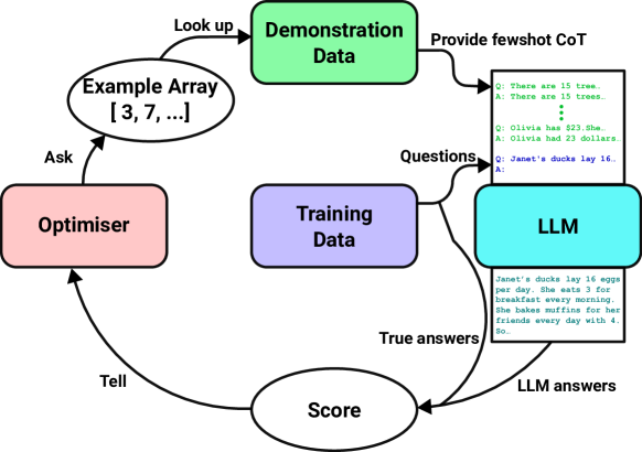
Figure 1. Overview of the proposed CoT optimization process.

Overview of the proposed CoT optimization process.

In line with previous works, we investigate the effect of few-shot prompting through automated example selection. However, we use these examples as a pre-prompt for the whole downstream task at hand: once constructed, these few examples remain fixed for the given task (here, mathematical modeling (Feigenbaum et al., 1963; Bundy, 1983)). This differs from various in-context learning methods (see Section 7) in which the selection of the prompts depends on each specific instance. Furthermore, since most reasoning benchmarks provide a training set too small for proper training (Ni et al., 2023; Liu et al., 2023), we focus on evolutionary algorithms, which can be comparison-based and therefore only need a few bits as feedback, paving the way to information-theoretic generalization guarantees. We analyze mathematically the risk of overfitting or exploitative behavior of our evolutionary approach, and prove generalization bounds that do not exist for other approaches accessing fine-grain data with gradient-based methods.

Such an Evolutionary Pre-Prompt Optimization strategy (termed EPPO in the following) effectively identifies a concise set of examples (called for short few-shot in the following) that notably enhance performance when used together as pre-prompt. Additionally, considering the current limited understanding of few-shot mechanisms (Min et al., 2022), the insights gained from the selected examples enable us to identify new ways to improve LLMs performances, not only helping in the practical use of LLMs for complex tasks but also contributing to a better understanding of the nuances of few-shot prompting at large.

The paper is organized the following way: Section 2 introduces the different components of EPPO and details the algorithm itself. Section 3 proposes information-theoretic results and proves some generalization bounds (Section 3.2) for EPPO thanks to the limited information it requires to optimize the pre-prompt. Section 4 presents the experimental validation of EPPO with an emphasis on overfitting, while Section 5 digs deeper inside its working details. Section 6 discusses these results, and Section 7 puts them in perspective with other related published works. Finally, Section 8 summarizes and concludes the paper.

2. Methods

This work focuses on optimizing the performance of a given LLM on a given complex downstream task (e.g., mathematical reasoning) through few-shot CoT pre-prompting. Our primary goal is to identify the most impactful small pre-prompt that can significantly boost the LLM performances on the task at hand, i.e., to select a small set of prompts from a given demonstration dataset $\mathcal{D}$ that, when used as pre-prompt for all further queries, improve the efficiency and effectiveness of the LLM on that task.

2.1. Few-shot optimization

For a given training set $\mathcal{T}$ and its corresponding demonstration set $\mathcal{D}$ made of CoT prompt examples, or simply CoT prompts (see Section 2.2), we aim to find out the best performing small subset, referred to as few-shot pre-prompt in the following, or simply pre-prompt. To do so, we formulate this problem as a combinatorial optimization problem, as follows (Figure 1):

• Representation of CoT prompt: Each example in the demonstration set $\mathcal{D}$ is assigned a unique index in $\{1,\dots,|\mathcal{D}|\}$. This transforms the demonstration set into a lookup table. Instead of searching in $\mathcal{D}^{s}$ (with $s$ the size of the few-shot prompts we are looking for), we search in $\{1,2,\dots,|\mathcal{D}|\}^{s}$.

• Construction of the few-shot pre-prompt: A few-shot pre-prompt is hence represented by a (small) list of $s$ integers (typically $2\leq s\leq 16$), each representing a CoT prompt from the demonstration dataset $\mathcal{D}$.

• Optimization: The objective is to identify the combination of integers (i.e., of CoT prompts) that maximizes the LLM performance for the task at hand on the training dataset. This involves varying the integers of the list (and possibly the order and the size of the list). This is amenable to black-box optimization (see Section 2.3).

• Evaluations: Every few-shot pre-prompt proposed by the optimization algorithm is tested on the dataset: The objective function for the black-box optimization is the performance of the LLM for the tasks at hand, which measures how well the chosen combination of CoT prompts works when used as a pre-prompt for the whole task.

2.2. Datasets construction

In our research setup, we work with training datasets that typically contain several thousand examples. However, optimizing various few-shot across the entire dataset is cost-prohibitive due to computational limitations and the high cost of running LLMs. Addressing this challenge, hence, required to employ a sub-sampling strategy. When datasets are categorized with various difficulty levels, we ensure a balanced approach by layered sub-sampling, i.e., uniformly sub-sampling across all categories and levels. This method guarantees a diverse range of examples in the reduced dataset, which is crucial for a comprehensive model evaluation.
In scenarios where the datasets lack such detailed categorization, we pivot to a strategy based on the uncertainty of the LLM responses, specifically when using LLaMA2-70B (Touvron et al., 2023). We generate $n$ different answers for each example, using a predefined temperature setting $\tau$, that influences the diversity of the model responses. In order to gauge the confidence in an answer, we analyze the frequency of the correct answer within these multiple responses. The idea is that the more frequently a correct answer appears, the higher the confidence of the model in that answer. Based on this confidence measure, we perform uniform sub-sampling across all levels of uncertainty. In practice, in our experiments, we take $n=10$ and take the same number of examples for each frequency of correct answers (in each bracket between $\frac{0}{10}$, $\frac{1}{10},\ldots\frac{9}{10},\frac{10}{10}$). This method allows us to select a representative subset of examples that captures a wide range of the model certainty levels as a proxy for the example difficulty.
The same strategy is used to build the demonstration datasets, starting from the remaining examples of the original training set. To further increase the demonstration diversity, we also add correct demonstrations generated by the model with the baseline CoT. As a result, the demonstration dataset $\mathcal{D}$ contains both hand-annotated and automatically generated demonstrations, limiting the need for human intervention.

2.3. Evolutionary optimization

The goal is to optimize an array of integers (the list of indices of query/answer pairs from the demonstration set): This is amenable to a classical black-box optimization scenario, allowing us to use standard optimization libraries like Nevergrad (Rapin and Teytaud, 2018). The simplest optimization algorithms for doing so consist of mutating the variables one or a few at a time, with possibly Tabu lists (though not used here). More sophisticated methods include selecting the variables or the number of variables to modify. This last option is frequent in recent works and included in Nevergrad algorithms such as “LogNormal” (Kruisselbrink et al., 2011) and “Lengler” (Doerr et al., 2019; Einarsson et al., 2019). In a nutshell (see e.g.,  (Rapin and Teytaud, 2018) for details), the following optimization algorithms are used in our experiments Section 4:

• The simple Discrete $(1+1)$-ES mutates each variable with probability $1/d$, in dimension $d$ (repeat if no variable is mutated): The mutated point is used as a new reference if its objective value is not worse than the previous best.

• The Portfolio method (Dang and Lehre, 2016) replaces $p=1/d$ with a uniform random choice of the mutation probability $p$ in $[0,1]$.

• The DoubleFastGA method is an adaptation in (Rapin and Teytaud, 2018) of the Fast GA(Doerr et al., 2017) to non-binary discrete variables.

• In the Lengler method, the mutation probability $p$ decreases over time, with a schedule that is mathematically derived for optimal performance on artificial test functions (Einarsson et al., 2019). Variants are included with variations of the critical hyperparameters: We refer to (Rapin and Teytaud, 2018) for details.

• The LogNormal method (Kruisselbrink et al., 2011) uses a self-adaptation mechanism that modifies the mutation probability $p$, that is itself subject to log-normal mutation.

• Some variants of these algorithms are also tested (their name contains “Recombining” or “Crossover”) with a crossover operator. The different crossover operators include (a) one-point crossover, (b) two-point crossover, and (c) recombining as in differential evolution, i.e., each variable is independently copied from a random parent. We do not check for duplicates in the list after the crossover, which is unlikely to happen thanks to the large size of the demonstration set $\mathcal{D}$ compared the few-shot size $s$.

• We also compare EPPO with random search, in which all variables are repeatedly and uniformly drawn in their domain, retaining, in the end, the overall best-encountered solution.

The discrete algorithms discussed above are generally presented in the context of binary variables, but the adaptation to categorical variables is straightforward: The mutation operator replaces the current value with a value that is randomly drawn in the domain of this variable (excluding the previous value).

2.4. Evolutionary Pre-Prompt Optimization

1:$Algo$ $\triangleright$ a comparison-based optimization algorithm with ask-and-tell interface

2:$\omega$, $b$ $\triangleright$ Random seed and budget

3:$\kappa\leftarrow Algo.initialize(\omega,b,\dots)$ $\triangleright$ $\kappa$: number of values returned by ask()

4:$Archive\leftarrow\emptyset$

5:for step $s$ in $1,\dots,b$ do

6:     $p_{1},p_{2},\dots,p_{\kappa}\leftarrow Algo.ask()$ $\triangleright$ the $\kappa$ pre-prompts to evaluate and compare

7:     $Archive.add(\{p_{1},\dots,p_{\kappa}\})$ $\triangleright$ store them in the archive

8:     $best(s)=Compare(p_{1},\dots,p_{\kappa})$ $\triangleright$ Run the LLM with each pre-prompt and

9:      $\triangleright$ return the index of the best

10:     $Algo.tell(best(s),p_{1},\dots,p_{\kappa})$ $\triangleright$ Only feedback: the result of the comparison

11:end for

12:return $r=Algo.recommend(Archive)$ $\triangleright$ return the best guess from the archive

Algorithm 1 EPPO global view. $Algo$ (specified by $ask$, $tell$, $recommend$) can be anything provided that $tell$ accepts a first argument $p_{best}$ in $\{1,\dots,\kappa\}$.

A global overview of EPPO algorithm is given in Figure 1 and its pseudo-code in Algorithm 1. Its main parameter is a comparison-based combinatorial optimization algorithm $Algo$, that handles categorical variables and uses the ask-and-tell interface (or a slight variant of it to take into account that it is comparison-based): It is initialized (3) with the random seed, the available budget, and any other useful information related to the problem at hand (e.g., number of variables with their domain of definition, constraints, etc). An archive of all visited points (points are pre-prompts here) is maintained (4). In the main loop, $Algo$ is asked for new points to evaluate (6). These points are added to the $Archive$ (7) and compared (8), the index of the best one being the only feedback given to $Algo$ (10). When the budget $b$ is exhausted, the best recommendation (usually the best pre-prompt from $Archive$, but possibly another one, for instance, on noisy problems) is returned as the proposed optimal solution (12).

The formalization using $\kappa$ departs from the usual formalism of Evolutionary Algorithms but aims to cover most possible cases. It covers at least all the algorithms used in this work and is described in Section 2.3. It will be necessary for the derivation of the theoretical results in Section 3, based on information theory. It represents the number of points that $Algo$ will send for comparisons. In particular, it can include or not the previous current point of the algorithm and can also include a full population. For instance, for $(1+\lambda)$-ES, it is $\kappa=1+\lambda$ while for $(1,\lambda)$-ES, it is $\kappa=\lambda$.

Finally, $Compare(p_{1},p_{2},\dots,p_{\kappa})$ (8) runs the LLM on the training data using each $p_{i}$ in turn, as can be visualized on the right part of Figure 1. It then typically (though our proof does not assume anything except Equation 5) returns its estimation of the best-performing pre-prompt. Typically, EPPO can be seen as a repeated A/B pre-prompt testing scenario of an online LLM, but without ensuring that the same questions are sent to both alternatives nor that we have access to a detailed ground truth answer for each question.

Next, Section 3 analyzes in more depth the properties of EPPO and derives bounds on the generalization error in the case of few-shot pre-prompts (i.e., containing only a small number of examples from the demonstration set). Our key result is that, thanks to information theory and the nature of our algorithms (which all verify an equation of the form Equation 5 as they are based on comparisons and not on detailed losses or gradients), we can derive generalization bounds. Liu et al. (2023) has emphasized how hard it is to train an LLM on a small training set such as GSM8k, even with a small LLM. We show that we can do such a training even with a LLaMA2-70B model.

3. Information-theoretic analysis

In modern deep learning, it is increasingly common for test datasets to be inadvertently contaminated by data from the training phase: LLMs being pre-trained on almost the entire Internet, it is possible, and even probable, that the pre-training data leaks some of the test data (Li, 2024). Furthermore, fine-grain data can lead to various issues, such as over-exploitative behaviors (Zheng et al., 2024).

Therefore, overfitting becomes critical (Mirzadeh et al., 2024; Yang et al., 2024), and making progress in the direction of reasoning might require new types of learning focused on generalization (Mitchell et al., 2023; McCoy et al., 2023; Dziri et al., 2023; Berglund et al., 2024). We will now discuss how EPPO is a priori less prone to overfitting than its competitors by requiring feedback with limited information (specifically, using only comparisons from possibly big datasets).

3.1. Data size and usage

Various approaches have been proposed for improving LLMs. Some examples include Reinforcement Learning from Human Feedback (RLHF) (Lee et al., 2023; Abramson et al., 2022; Jain et al., 2015); direct usage of the human feedback (Videau et al., 2023; Kim et al., 2023); reward modeling (Adams et al., 2022) to reduce data usage; and tuning only a small part of the models (Lu et al., 2022a; Giannou et al., 2023; Burkholz, 2024). On the opposite, EPPO uses little (binary, or more generally $\kappa$-ary) information that is coarse-grain (aggregated over an entire dataset and not on mini-batches) in order to tune a small pre-prompt (array of prompts from the demonstration set, typically, 2 to 16 indices in $[0,999]$). Table 1 summarizes the size and use of data of the different approaches listed above to train and improve LLMs.

Indeed, let us consider in Algorithm 1 the simplest case where $\kappa=2$ (e.g., $Algo$ is a variant of a (1+1)-ES), and let us compute the size of the feedback sent to the optimization algorithm $Algo$ during one run of EPPO. When $\kappa=2$, at each iteration, one comparison is performed by the $Compare$ routine (8), and there are $b$ iterations (see Figure 2). Hence the entire data flow used as feedback is exactly $b$ bits. The general case for $\kappa$ will be discussed in the forthcoming  Section 3.2.

Furthermore, EPPO never makes any backward passes, which does bring a lot of information to the model, nor does it send data as mini-batches, which would also multiply the information integrated in the model. Paradoxically, whereas classical deep learning methods try to avoid underfitting by integrating as much information from the dataset as possible into the model, EPPO focuses on decreasing overfitting by using a limited data flow.

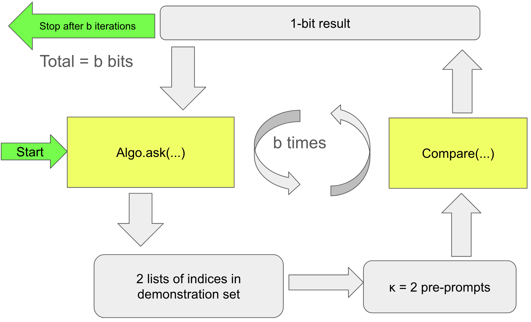
Figure 2. EPPO from the information-theoretical point of view in the case $\kappa=2$: The loop is used $b$ times, and 1 bit (the result of a comparison) is returned and used at each iteration. The total information flow in the top left arrow is hence $b$ bits.

EPPO from the information-theoretical point of view in the case $\kappa=2$: The loop is used $b$ times, and 1 bit (the result of a comparison) is returned and used at each iteration. The total information flow in the top left arrow is hence $b$ bits.

Table 1. Information used for various approaches. For LLM training (resp. fine-tuning), $n$ (resp $n^{\prime}$) is the number of prompts in the training (resp. fine-tuning) set, $s$ their typical length, $i$ the typical input length, $o$ the typical output length ($i$ and $o$ in the dozens or hundreds of scalars); RLHF, uses tens of thousands of human answers times the input length; For EPPO (Algorithm 1), $b$ is the budget, and $\kappa$ the “population” size of the optimizer: In the case $\kappa=2$, these $b$ scalars are Booleans.

Context	Type of	Data	Orders of	Generalization
	data	volume	magnitude	bound
LLM training	Complete Seq2Seq	$n\times s$ chars	$\simeq 10^{12}$	-
Fine-tuning	Complete Seq2Seq	$n^{\prime}\times(i+o)$ chars	$\simeq 1e6$ for GSM8K	-
	Questions
RLHF	and selected answer	$n^{\prime}\times(i+1)$ chars	frequently $10^{6}$	-
	Scores of $b$			$\delta_{EPPO}=O(\kappa^{b})$
EPPO	pre-prompts	$b$ scalars	$\simeq 100$	(Equation 7)

In next Section 3.2, we will theoretically validate the use of such a limited data bandwidth in EPPO by deriving the resulting mathematical bounds on the generalization error, while the results of Section 4 will provide its experimental validation.

3.2. Mathematics of overfitting

Following (Fournier and Teytaud, 2011), this section derives proven upper bounds on the generalization error of EPPO. Let us first define what we mean by generalization error.

Notations: For a given $\varepsilon>0$, let us denote $err_{\varepsilon}(p)$ the event that the difference between the empirical risk (loss computed on the whole training set) and the risk in generalization (expected loss on the full space, of course unreachable) is greater than $\varepsilon$:

$$err_{\varepsilon}(p)=\{|(expected\ loss\ of\ p\ in\ generalization)\ -\ (empirical\ loss\ of\ p\ on\ dataset)|>\varepsilon\}$$

We are interested here in bounding, for any $p$ returned by EPPO, the probability of this event, aka a large deviation of the generalization error of pre-prompt $p$.

Hypothesis: We assume that for all $\varepsilon>0$, there exists $\delta>0$ such that for all $p\in\mathcal{D}^{s}$,

(1) $$P(err_{\varepsilon}(p))\leq\delta.$$

This bound is non-trivial only if $\delta<1$, and further results will depend on $\delta$.

An example of such a deviation bound is the case where the evaluation of a pre-prompt is based on averaging $T$ distinct, independent answers of the model, where $T$ is the size of the training dataset $\mathcal{T}$: For each question, the answer receives a score in $[0,1]$. Then by Hoeffding’s inequality, we have

(2) $$\delta=P(err_{\varepsilon}(p))\leq 2\exp(-2T\varepsilon^{2}).$$

But we do not need this specific bound and only suppose here Equation 1.

Goals: The challenge is to extend Equation 1 to one of the following settings:

• for the pre-prompt $r$ recommended by EPPO, which is unknown a priori (in the same spirit as (Vapnik, 1995)), we look for some $\delta_{EPPO}>0$ such that:

  (3) $$P(err_{\varepsilon}(r))\leq\delta_{EPPO}.$$

  The difficulty is that $r$ is not known in advance, so Equation 1 does not immediately provide  Equation 3.

• A useful extension consists in bounding the risk that at least one of the pre-prompts considered in Algorithm 1 (all those stored in $Archive$) has a deviation of more than $\varepsilon$ by some $\delta_{unif}>0$, i.e.,

  (4) $$P(\exists p\in Archive,err_{\varepsilon}(p))\leq\delta_{unif}.$$

  The advantage of this extension is that we not only guarantee a deviation for the final recommended $r$ but also for all pre-prompts considered during the run. And because the optimization algorithm $Algo$ and the tool $Compare$ use $\kappa\times b$ different pre-prompts, which are not chosen a priori, Equation 4 can not be immediately derived by a Bonferroni correction.

Preliminary:

• Everything else being equal (training and demonstration sets, $Algo$ and budget $b$ in Algorithm 1), a given $p$ only depends on the random seed $\omega$ that was used in the run of Algorithm 1 that returned it. We will hence start reasoning for a given $\omega$, then generalize to all possible $\omega$ to get bounds on the generalization of EPPO as a whole.

• The key feature here is that the function $Compare()$ (8 in Algorithm 1) is based on an evaluation of the pre-prompts and returns an index in $\{1,\dots,\kappa\}$:

  (5) $$Compare(\dots)\in\{1,\dots,\kappa\}.$$

Proof: We now mathematically prove, following (Videau et al., 2024), that, in terms of statistical risk, this leads to a bound on the generalization error.

First, consider a specific random seed $\omega$. We can apply the Bonferroni correction (Bonferroni, 1936): Consider a list $\mathcal{L}$ of $M$ pre-prompts. Assuming Equation 1, the risk of deviation greater than $\varepsilon$ for at least one of those pre-prompts is at most $M\cdot\delta$ instead of $\delta$:

(6) $$P(\exists c\in{\mathcal{L}},err_{\varepsilon}(c))\leq M\delta.$$

Consider now the complete list $\mathcal{L}$ of pre-prompts that could be returned by Algorithm 1 (12). $Compare(\dots)$ has only $\kappa$ possible values (Equation 5). Hence the pre-prompt chosen at the end is in the list $\mathcal{L}$ of $\kappa^{b}$ pre-prompts – and this list only depends on the random seed $\omega$. Then, applying Equation 6 leads to

(7) $$P(err_{\varepsilon}(r))\leq\kappa^{b}\delta,$$

where $r$ is the value returned by Algorithm 1. This solves our quest for an equation of the form of Equation 3: we have proved that EPPO returns a pre-prompt $p$ with a limited generalization error, i.e., the empirical evaluation should not be too far from the performance in generalization. $\blacksquare$

Discussion: One should be aware that a lower bound on the generalization error of an algorithm has no connection with its accuracy. Indeed, consider, for instance, the case of pure random search, in which a randomly drawn few-shot (made of $s$ examples) is drawn from ${\mathcal{D}}^{s}$ at each iteration, regardless of the past. $Algo.ask()$ always returns one independently randomly drawn pre-prompt, and $Compare(\ldots)$ is not called at all: We can consider that $\kappa=1$. However, for the last step, all those randomly drawn pre-prompts are compared once, and the best one is returned: For that step, $\kappa=b$ there. Therefore, the total number of possible recommended pre-prompts is $1^{b-1}\times b$, hence $b$, for Random Search:

(8) $$P(err_{\varepsilon}(r))\leq b\delta,$$

Compare this to $\kappa^{b}$ in Equation 7: EPPO with Random Search overfits less than EPPO with evolutionary search. On the other hand, of course, it performs worse than evolutionary based variants in terms of finding empirically good pre-prompts. We discuss this in Section 4.4: A straightforward next step (discussed in (Videau et al., 2024)) would be to search for a trade-off between the search effectiveness of evolutionary algorithms and the generalization ability of Random Search by using evolution with a much larger population.

We now consider two straightforward extensions of Equation 7.

Extension with stochasticity: We derive the previous results in the context of a fixed random seed $\omega$. If the algorithm is randomized (i.e., $\omega$ is actually randomly chosen), this bound is still valid: The risk of deviation by more than $\varepsilon$ (averaged over all these random outcomes) is the average of the different risks corresponding to the different random outcomes (in mathematical terms, $P(err_{\varepsilon}(r))={\mathbb{E}}_{\omega}P(err_{\varepsilon}(r)|\omega)$), and the same bound applies to the average.

Bound over more pre-prompts: Instead of proving a bound valid for all $p$ in the possibly recommended pre-prompts (and therefore valid for the $r$ returned by Algorithm 1), we could consider a bound valid uniformly over all $p$ considered in all the $Compare(\dots)$ of the algorithm, i.e., in all $Archive$. This implies that the optimization algorithm works on correctly estimated few-shot. Given that our bound is computed by uniformity over all possible outcomes $\in\mathcal{L}$, the extension to all $Archive$ is straightforward: We need to slightly modify the constant in Equation 9 and replace $\kappa^{b}$ by $\kappa^{b+1}$. This solves our quest for an equation of the form Equation 4. $\blacksquare$

We observe that the risk of a deviation greater than $\varepsilon$ is limited by $\kappa^{b}\cdot\delta$, which increases when the computational budget $b$ increases. Also, the risk decreases with $\delta$, i.e., if the precision for each model individually increases, e.g., if the training set size $T$ increases: Overall, assuming a bound as in Equation (2), we get a risk as in Equation (9), or, in other words, a precision $\varepsilon$ as in Equation (10):

(9) $$\delta \leq 2\kappa^{b}\exp(-2T\varepsilon^{2}),$$

(10) $$\varepsilon \leq \sqrt{-\frac{\ln(\kappa^{-b}\delta/2)}{2T}}.$$

4. Experimental Results

This section presents the experimental validation of EPPO on several mathematical reasoning tasks.

Table 2. LLaMA2-70B: 3 baselines at the top, then 2-shots, 4-shots and 8-shots optimization and the best prompt of the 7B transferred to 70B. We observe that (i) 4-shots is best (ii) transferring the preprompt from 7b does work, though few-shots optimization is better. For MathQA, without parentheses, the exact match for the numerical answer and choice of the right option between parentheses.

Prompt Type	GSM8k		SVAMP		MathQA		MATH
	# Tokens	Acc.	# Tokens	Acc.	# Tokens	Acc.	# Tokens	Acc.
CoT	762	56.8	762	73.1	602	25.4 (35.8)	671	13.9
Long CoT	2838	66.5	2838	74.7	2019	21.9 (29.9)	1435	14.2
Resprompt	2470	65.7	2470	71.0	1367	9.9 (13.0)	-	-
EPPO 2	412	62.5	412	75.0	406	26.6 (35.6)	843	14.0
EPPO 4	1297	68.2	1297	78.3	906	34.1 (41.0)	1587	15.4
EPPO 8	1651	67.6	1651	77.3	1651	30.5 (39.1)	1634	14.7
7B $\rightarrow$ 70B	809	64.7	809	76.4	888	27.2 (31.4)	641	14.3

4.1. Experimental settings

Datasets: EPPO is evaluated on four mathematical reasoning tasks. Each task comes from a different dataset and they have heterogeneous complexity. The datasets used here are GSM8k (Cobbe et al., 2021), SVAMP (Patel et al., 2021), MathQA (Amini et al., 2019), and MATH (Hendrycks et al., 2021). GSM8k and SVAMP focus on real-world mathematical problems. While GSM8k offers a comprehensive training set, SVAMP does not have a corresponding training set. To tackle this issue, we will test the transferability of EPPO by evaluating on SVAMP the same few-shot pre-prompts found for GSM8k. MathQA offers a wide range of mathematical problems of varying difficulties. In contrast, MATH poses the greatest challenge, targeting advanced mathematics typically encountered in late high school and beyond. Also, notice that MathQA has very noisy annotations, and hence provides a test for the resilience of optimization strategies. For an in-depth understanding of each of these datasets, including specifics about their training, demonstration, and test components, please refer to Table 7 in the Appendix.

Evaluation metrics: For each dataset, our primary metric is the exact match (EM) with the ground truth. Specifically, we focus on the final output generated by the model, which is typically a numerical value, and we compare it directly with the ground truth. In the case of the MathQA dataset, which involves multiple-choice questions, we use two distinct EM scores: one for the numerical answer and another for the correct multiple-choice option (identified simply by its letter). This dual-scoring approach is particularly beneficial for evaluating smaller/less capable models that do not effectively correlate with the numerical answer.

Language models: We use the LLaMA family of models (i.e., LLaMA2 (Touvron et al., 2023)). A key advantage of these models is their open-source nature, which significantly helps conduct cost-effective and reproducible research.

Baselines: The baselines used for comparison are: (a) the original CoT prompt (Wei et al., 2022b), as detailed in the publication and sourced from their appendix; (b) the Long CoT prompt (Fu et al., 2022) that includes examples with more steps, targeting complex reasoning tasks. These prompts were obtained from the official GitHub repository; and (c) the Resprompt approach (Jiang et al., 2023) that suggests following a reasoning graph and adding residual connections between the nodes of the graph. This technique is designed to reduce errors in multi-step reasoning tasks by LLMs. We sourced the Resprompt prompts from the paper appendix.

We do not include in-context learning such as (SU et al., 2023; Wu et al., 2022; Zhang et al., 2023a; Gupta et al., 2023; Ye et al., 2023; Rubin et al., 2022), which optimize a pre-prompt on a per-example basis. Likewise, they are usually tested on heterogeneous and older models without considering mathematical reasoning tasks. Moreover, their source codes are barely available.

For MATH tasks, which are not covered by any of the baselines, we took the base CoT prompt from Minerva (Lewkowycz et al., 2022). For the Long CoT, we created prompts using the most detailed and complex answers from the training set. All these baselines prompt are 8-shot for GSM8k and SVAMP, 4-shot for MathQA and MATH. To ensure a fair comparison, we run all these baseline prompts in our own codebase. Our scores are consistent with the original papers, except in the case of Resprompt for which we get worse results on MathQA.

Hyperparameters: For each task, except for SVAMP, which lacks a training set, we create a smaller training set containing roughly 500 samples by downsampling the original one, and assemble a demonstration dataset of about 1000 samples, as described in Section 2.2. Precise details about each dataset can be found in Table 7 in the Appendix. In Algorithm 1, the optimization algorithm $Algo$ is chosen among those described in Section 2.3, in their Nevergrad implementation (Rapin and Teytaud, 2018); The budget $b$ is set to 100 for both the LLaMA2-7B and LLaMA2-70B models; The number $s$ of prompts from the demonstration set $\mathcal{D}$ is taken in $\{2,4,8,12,16\}$, and such pre-prompts are denoted for short “$s$-shot pre-prompts”.

4.2. Results on Few-Shot Optimization

Table 3. LLaMA2-7B: 3 baselines at the top, then 2-shots, 4-shots, and 8-shots optimization, and the best pre-prompt of the 70B transferred to 7B. We observe that (i) 4-shots is best, (ii) no improvement when transferring the pre-prompt from 70B to 7B.

Pre-prompt Type	GSM8k		SVAMP		MathQA		MATH
	# Tokens	Acc.	# Tokens	Acc.	# Tokens	Acc.	# Tokens	Acc.
CoT	762	14.1	762	39.6	602	10.1 (19.8)	671	3.3
Long CoT	2838	17.5	2838	35.9	2019	9.4 (17.5)	1435	3.0
Resprompt	2470	16.9	2470	30.4	1367	6.7 (13.8)	-	-
EPPO 2-shot	582	16.4	582	39.6	442	9.9 (17.6)	460	4.5
EPPO 4-shot	809	15.5	809	41.6	888	14.7 (19.4)	641	3.9
EPPO 8-shot	2088	16.5	2088	39.4	1945	12.3 (16.7)	1254	3.7
EPPO 70B $\rightarrow$ 7B	412	12.4	412	40.5	888	8.5 (14.5)	843	2.6

Our results, detailed in Tables 3 and 2, showcase the performance of EPPO across different tasks for both the LLaMA2-7B and LLaMA2-70B models. We evaluate our approach on different $s$-shot setup with $s\in{2,4,8}$, to understand its effectiveness in various contexts. As one can see in both tables, the results consistently indicate that EPPO outperforms all baselines. This improvement is noteworthy not only in terms of accuracy but also in terms of efficiency, as indicated by the similar or even reduced number of tokens in the few-shot pre-prompts used. This reduced number of tokens is directly reflected in a reduced inference cost, both in memory and computation time. Furthermore, an important aspect of their results is the versatility of EPPO. It is effective across models of different sizes, from the smaller LLaMA2-7B to the larger LLaMA2-70B. Interestingly, we observe more pronounced gains in performance with the larger model. This suggests that EPPO scales well and can leverage the increased capacity of larger models.

Per example complexity results: This analysis, detailed in Figure 7, examines the number of correct solutions across different levels of problem complexity for LLaMA2-70B: EPPO consistently outperforms baseline methods across numerous complexity levels. This is particularly noteworthy for more complex problems, where EPPO delivers better results, even though it was not specifically designed for such challenging scenarios. The most pronounced improvements are observed for the GSM8k and MATH tasks, especially on multi-step examples, which are typically harder to enhance (Fu et al., 2022). These gains are achieved without any deliberate focus on such difficult problems during either the optimization process or within the demonstration dataset. This outcome demonstrates the strong generalization ability of EPPO in adapting to and addressing complex challenges without specifically targeting them beforehand.

Task Transfer: As said, our approach to SVAMP, in the absence of a specific training set, involves applying few-shot pre-prompts optimized for GSM8k. This strategy leads to a notable and consistent improvement over the existing baselines across all few-shot settings. Notably, while methods like Resprompt, designed to enhance multi-step reasoning, struggle to adapt to the simpler SVAMP task, EPPO demonstrates more flexibility. It successfully transfers to SVAMP and simultaneously improves performance in multi-step reasoning tasks. Further details on task transferability for LLaMA2-70B, using GSM8k optimized 4-shot pre-prompts, are available in Table 9 in the appendix.

Model transfer: We investigate the transfer of optimized pre-prompts between two models, LLaMA2-7B and LLaMA2-70B, on the same task. We optimize pre-prompts with EPPO on one of these LLMs, and test it on the other one. For LLaMA2-70B, we use optimized 4-shot pre-prompts, and for LLaMA2-7B, we choose the best from either 4-shot or 2-shot pre-prompts. The results of this experiment are presented in Tables 3 and 2. Table 3 shows the performance on the LLaMA2-7B model using pre-prompts optimised for LLaMA2-70B (indicated as 70b $\rightarrow$ 7b), and Table 2 displays the results on the LLaMA2-70B model of pre-prompts optimised for LLaMA2-7B (indicated as 7b $\rightarrow$ 70b). From these results, we observe that pre-prompts optimized for the larger LLaMA2-70B model do not effectively transfer to the smaller LLaMA2-7B model. Interestingly, the opposite scenario – transferring pre-prompts from LLaMA2-7B to LLaMA2-70B – resulted in a substantial performance increase, surpassing some of the baselines. Nevertheless, pre-prompts that were specifically optimized for one model always outperform pre-prompts that are transferred from the other model.

Effect of the number of shots on performance: Each model is tested with few-shot optimized pre-prompts containing 2, 4, and 8 shots. We observe that using more than four examples does not lead to better results in the downsampled case. In fact, it appears that employing more than four examples in a pre-prompt can slightly but steadily degrade the performance of the LLM. This is a counter-intuitive finding, as one might intuitively assume that providing more examples in the few-shot pre-prompt would lead to broader coverage of the task, thereby improving the LLM’s ability to generate task-specific responses: hence the investigation below in terms of overfitting.

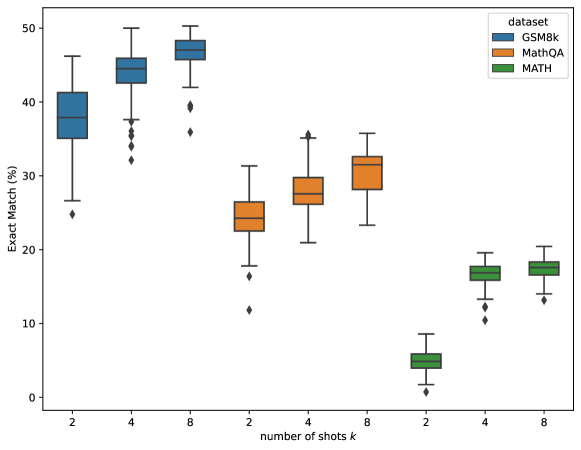
Figure 3. Comparison between 2-shot, 4-shot, and 8-shot: training score over the EPPO run for LLaMA2-70B: Each boxplot represents the loss values observed during the whole run. The numbers represent the percentage of exact matches on the training set. Typically, for each number of shots, the bottom part (low EM) corresponds to the beginning of the run, similar to random search, and the performance of these initial few-shot increases greatly with the number of shots.

Comparison between 2-shot, 4-shot, and 8-shot: training score over the EPPO run for LLaMA2-70B: Each boxplot represents the loss values observed during the whole run. The numbers represent the percentage of exact matches on the training set. Typically, for each number of shots, the bottom part (low EM) corresponds to the beginning of the run, similar to random search, and the performance of these initial few-shot increases greatly with the number of shots.

Effect of the number of shots on overfitting. In order to understand why we get better results with a small number of shots, whereas 8 shots are usual, we investigate the performance of LLaMA2-70B after running EPPO on the training set using 2, 4, and 8 shots for each task, scrutinizing the optimizer logs of the train error along optimization. Our findings are illustrated in Figure 3, showing statistics gathered over the full EPPO run, and in Table 5 presenting test errors. There is a noticeable and consistent performance gap between the 2-shot prompts and those with more than 4 shots in Figure 3. This indicates that increasing the number of shots from 2 to 4 yields most of the (train error) benefits. Also, with an increase in the number of shots, there was a corresponding increase in the median performance (median over the EPPO run) and in the performance of the worst-performing prompts (typically randomly generated at the beginning, before overfitting can take place). When considering the test error, Tables 5 and 4 show that increasing the number of shots, in the downsampled case, leads to a clear overfitting. We conclude that the problem of large few-shot is an overfitting issue, particularly visible in the downsampled case. This is confirmed by Table 6, which shows good results for larger few-shot when EPPO uses the full training set (without downsampling).

4.3. Experiments on the downsampled GSM8k

Table 4. Comparison between exact match accuracies (without SC) obtained with different discrete optimization methods with budget 100 on the training set. We observe a significant performance improvement compared to random search. Red for the 2 worst performances. Additional results in Table 5.

	LLaMA2-7B			LLaMA2-70B
	GSM8k num-shots
Optimizer	8-shot	4-shot	2-shot	8-shot
RandomSearch	13.0	13.0	13.3	46.6
LogNormal$(1+1)$	12.8	13.5	12.8	45.1
DoubleFastGA	15.0	14.8	14.3	51.0
Portfolio$(1+1)$	15.5	14.5	14.8	49.7
Discrete$(1+1)$	15.8	15.5	14.8	51.7
Lengler$(1+1)$	14.8	14.8	14.8	50.3

Table 4 presents a sanity-check comparison against pure Random Search of different optimization algorithms used within EPPO, applied to the downsampled GSM8k training set (1/16 of the complete set, see Section 2.2 for details). We observe a gap between the train (Table 4) and test (Table 6, Table 5, Figure 4) scores of Llama-70B on GSM8k, primarily due to the downsampling procedure, which leads to the different difficulty levels being more uniformly represented in the training set than in the test set. As said, we use the algorithms described in Section 2.3 in their Nevergrad implementation (Rapin and Teytaud, 2018): LogNormal (Kruisselbrink et al., 2011), DoubleFastGA (Doerr et al., 2017), Portfolio (Dang and Lehre, 2016), the basic Discrete ES, and Lengler (Einarsson et al., 2019); We refer to  (Doerr et al., 2019) for a theoretical analysis including the classical Discrete $(1+1)$-ES.

Most algorithms (except LogNormal) clearly outperform random search (in red), while Discrete (1+1)-ES performs best for all small-shot sizes (in bold): Given the high computational cost associated with an LLM inference, choosing an efficient optimizer plays an important role in managing computational costs more effectively.

4.4. Extension to the full training set: reducing the overfitting

Liu et al. (2023) pointed out how learning on the training set of GSM8k is hard due to the moderate size. We investigate in the present section to which extent EPPO is relevant for the training set of GSM8k. We mathematically proved in Section 3.2 that the overfitting should be low thanks to the limited access of EPPO to fine-grain data, but can be further limited by increasing the training set size $T$ (Equation 2). Figure 4 presents experimental results validating these theoretical findinds, and extending this claim with results both on one-sixteenth of the training set (downsampled GSM8k as in Section 4.3) on the left and on the entire training set (though still using only a single scalar indicator per few-shot pre-prompt) on the right: We emphasize positive results on GSM8k with positive transfer on SVAMP with just 50 to 150 bits of information from the data.

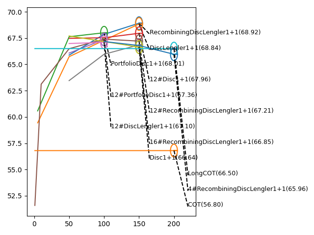
4, 8*, 12 or 16 shots,	4, 8*, 12 or 16 shots
Downsampled (1/16th) GSM8k	Full GSM8k

Figure 4. Results of Llama 70B, Exact Matches on the test set without improvement by Self-Consistency. Legends are the Nevergrad algorithm names pre-pended with ”s#” (*$s=8$ is the default few-shot size $s$, when not mentioned). For all algorithms, $\kappa=2$, so the x-axis is exactly the number of binary comparisons between pre-prompts, i.e., budget $b$ in Algorithm 1. Figure 5 presents the results of the transfer to SVAMP.
Left: Downsampled GSM8k. For $s\in\{12,16\}$, we observe a clear overfitting (confirmed with more experiments in Figure 12): The test performance decreases when the budget increases, consistently with the mathematical analysis. We also observe no overfitting for Random Search, which grows steadily with $s\in\{4,8,12,16\}$. Note that the longest run used 16 GPUs during $\simeq$ 30 hours.
Right: Full GSM8k. As only one bit of information is used per iteration (comparison with the best so far), we observe no overfitting until budget 150. Note that the longest run here used 160 GPUs during $\simeq$ 48 hours.

Results of Llama 70B, Exact Matches on the test set without improvement by Self-Consistency. Legends are the Nevergrad algorithm names pre-pended with ”s#” (*$s=8$ is the default few-shot size $s$, when not mentioned). For all algorithms, $\kappa=2$, so the x-axis is exactly the number of binary comparisons between pre-prompts, i.e., budget $b$ in Algorithm 1. Figure 5 presents the results of the transfer to SVAMP.
Left: Downsampled GSM8k. For $s\in\{12,16\}$, we observe a clear overfitting (confirmed with more experiments in Figure 12): The test performance decreases when the budget increases, consistently with the mathematical analysis. We also observe no overfitting for Random Search, which grows steadily with $s\in\{4,8,12,16\}$. Note that the longest run used 16 GPUs during $\simeq$ 30 hours.
Right: Full GSM8k. As only one bit of information is used per iteration (comparison with the best so far), we observe no overfitting until budget 150. Note that the longest run here used 160 GPUs during $\simeq$ 48 hours.

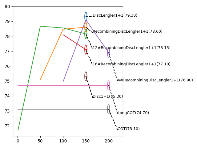
Figure 5. Transfer of pre-prompts optimized on full GSM8k (see caption of Figure 4-Right) to SVAMP. We observe a good transfer in this context.

Transfer of pre-prompts optimized on full GSM8k (see caption of Figure 4-Right) to SVAMP. We observe a good transfer in this context.

Generalization error: Random search vs other methods: Whereas Table 4 shows poor results for random search (in terms of training error), we observe (Table 5, left) that in generalization, when we have downsampled the GSM8k training set, overfitting matters more, and random search becomes competitive. This is consistent with the limited overfitting predicted by Equation (8).

Table 5. Random Search vs other optimizers, for budget $b=50$ and $100$. Bold for the best performances, red for worst. +/- denotes cases in which budget 100 outperforms (resp. underperforms) budget 50 (i.e., no overfitting). Observations: (1) the downsampled case is more prone to overfitting (much more “-”) (2) Random Search never overfits (consistently with predictions in Section 3.2) whereas other methods do, to the point random search is sometimes the best in the downsampled case (3) few-shot sizes 12, 16 are more prone to overfitting than 4, 8. The few missing values are on-going computations at the time of submission.

	Downsampled GSM8k				Full GSM8k
Few-shot size $\rightarrow$	4	8	12	16	8	12	16
Algorithm $\downarrow$
Budget 50: no overfitting & random search is weak
RandomSearch	64.13	64.68	64.13	62.16	66.41	66.33	60.72
Portfolio	64.80	64.80	65.57	65.54	67.62	66.07
Disc1+1	65.50	64.70	66.94	63.00	67.70	67.47
DiscLengler1+1	66.71	66.71	67.70	65.04	65.73	66.98
RecombDiscLengler	66.75	66.75	65.45		65.88	66.48	63.45
Budget 100: Overfitting matters & random search is competitive
in the downsampled case.
RandomSearch	66.33+	65.76+	66.33+	64.44+	65.95	67.09	62.69+
Portfolio	67.46+	67.46+	65.23-	62.62-	68.00+	67.36+
Disc1+1	66.18+	65.30+	66.07-	66.18+	67.53-	67.53+	65.69
DiscLengler1+1	66.77+	66.77+	65.95-	62.01-		67.09+
RecombDiscLengler	66.43-	66.43-	65.40-		67.85+	67.39+	65.95+

4.5. Combining with Self-Consistency

In the context of problem-solving with LLMs, multiple pathways often lead to a solution. Recognizing this, Wang et al. (2022) introduced the concept of self-consistency (SC) for LLMs. SC operates by generating a range of potential solutions with the same LLM. Diverse prompts for the problem at hand are generated by adding some random parts and controlling the level of randomness with a specific parameter $\tau$ called temperature. Each of these generated pathways leads to diverse answers that are then aggregated by a majority voting (Wang et al., 2022), effectively using the collective output of the model to determine the most likely correct answer.

We examine now the interaction between self-consistency, known for improving LLM performance, and pre-prompt optimization. The aim is to ascertain if the enhancements seen in single-path decoding also carry on to a self-consistency framework. Indeed, results presented in Table 6 show a clear benefit transferred from greedy decoding to self-consistency, at least with a temperature of 0.6 (a robust reasonable value, though sensitivity analysis remains to be done).

Table 6. Self-consistency improvement over optimized prompt and CoT baseline: error in test. The model tested here is Llama-2-70B with SC over 8 generations (maj@8) and temperature $\tau=0.6$.

Prompt Type	GSM8k	SVAMP	MathQA	MATH
Cot	56.8	73.1	25.4 (35.8)	13.9
CoT + SC	68.3	80.0	35.8 (44.9)	19.1
Downsampled training set
EPPO 4-shot	68.2	78.3	34.1(41.0)	15.4
EPPO  4-shot + SC	76.9	85.7	46.7 (50.4)	21.3
Full training set
EPPO  4-shot + SC	77.1	82.4	-	-
EPPO  8-shot + SC	79.1	85.5	-	-
EPPO  12-shot + SC	78.8	85.4	-	-

5. Insight Analyses

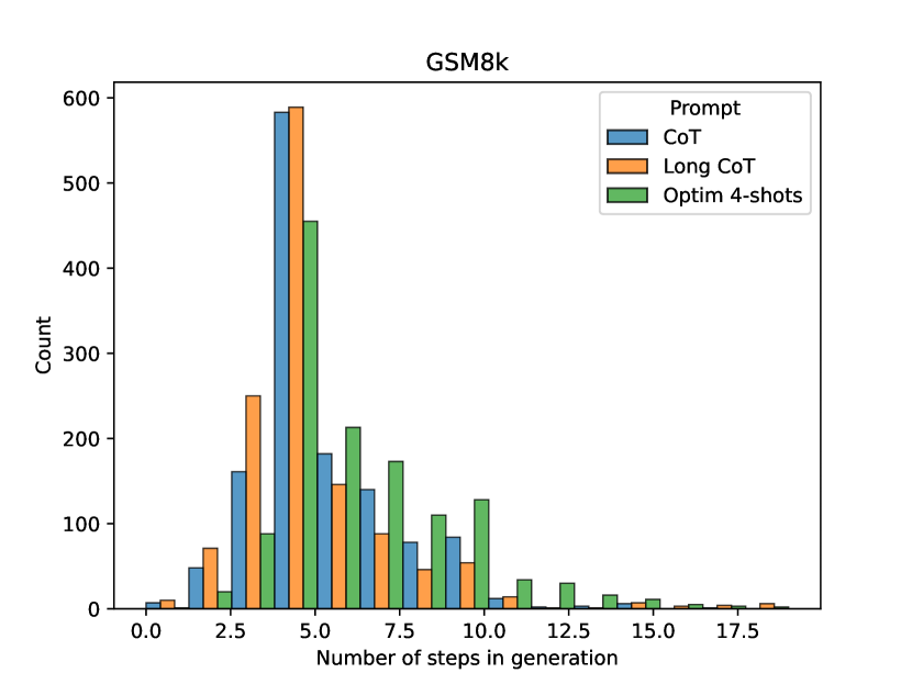
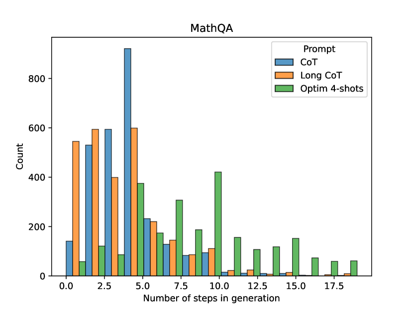
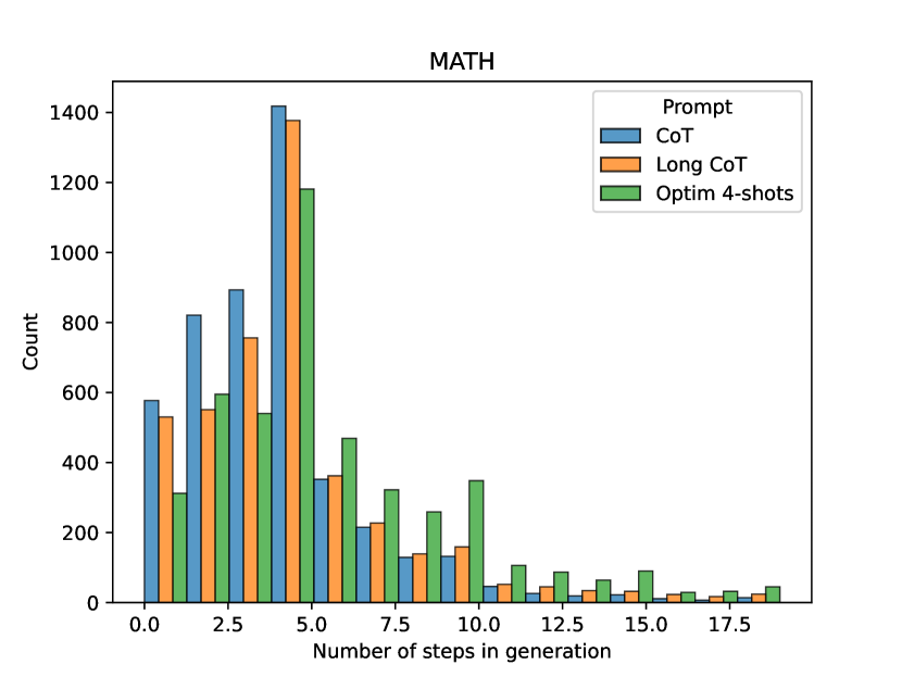
Figure 6. Comparison between the number of steps in the CoT, Long Cot, and EPPO for GSM8k (4-shot) and MathQA (8-shot) for LLaMA2-70B. The variance is higher for EPPO, with few-shot resulting in more steps in the output.

Comparison between the number of steps in the CoT, Long Cot, and EPPO for GSM8k (4-shot) and MathQA (8-shot) for LLaMA2-70B. The variance is higher for EPPO, with few-shot resulting in more steps in the output.

Effect of few-shot on LLMs generation: Figure 6 illustrate the number of steps generated by LLaMA2-70B across different tasks. As the number of steps to derive a solution can be hard to define, we use a simple method as a proxy: The number of steps is the number of sentences generated by the LLM to derive the answers. Contrary to baselines CoT and Long CoT, few-shot found by EPPO provide more diverse outputs in terms of number of steps. In particular, optimized few-shot pre-prompts tend to provide answers containing more steps. This extended number of steps might help to give better answers to multi-step examples (Figure 7).

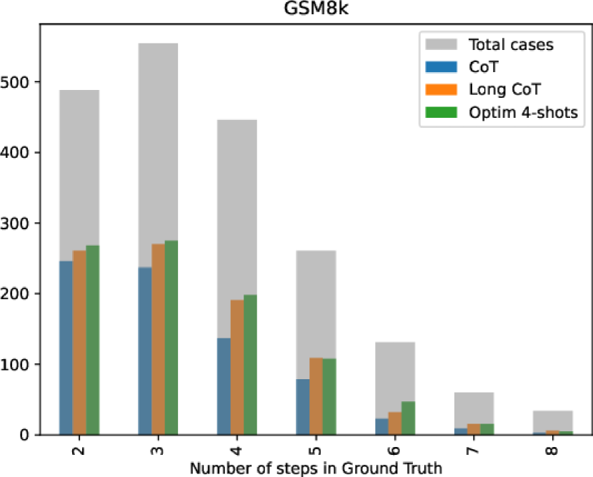
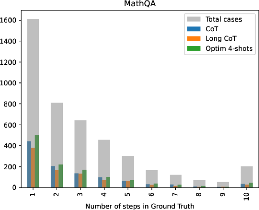
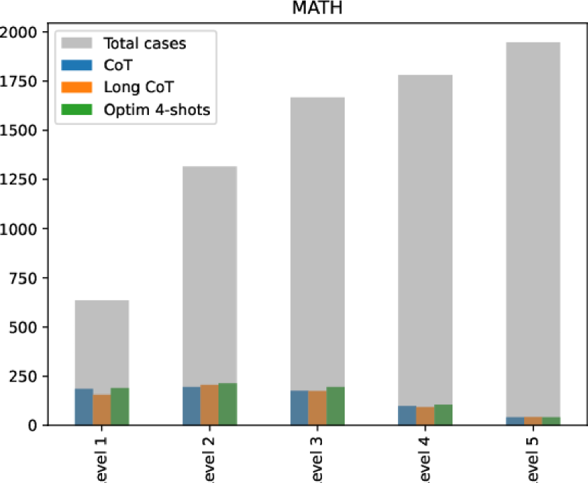
Figure 7. Exact Matches on LLaMA2-70B for CoT, Long Cot, and EPPO. X-axis: gold number of steps, i.e., number of steps in the ground truth or Level of the example for MATH: The x-axis is hence a measure of the complexity of problems. EPPO performs best in most cases.

Exact Matches on LLaMA2-70B for CoT, Long Cot, and EPPO. X-axis: gold number of steps, i.e., number of steps in the ground truth or Level of the example for MATH: The x-axis is hence a measure of the complexity of problems. EPPO performs best in most cases.

Operations on optimized pre-prompts: Here, we evaluate the robustness of the optimized few-shot prompts under various transformations: example permutations, removals, and combinations. Through these experiments, we seek to gain deeper insights into how a good few-shot pre-prompt is constructed. We perform this evaluation on GSM8k and MathQA. In this case, MathQA has been downsampled to 1000 samples to accelerate the evaluation.

Robustness against permutation: Figure 8 presents an analysis of how the performance fluctuates with changes in the order of few-shot prompts. To conduct this analysis, after running EPPO, we randomly modified the order of the prompts in the optimized pre-prompts ten times and observed the impact on the model performance in terms of Exact Matches.

(a) LLaMA2-70B

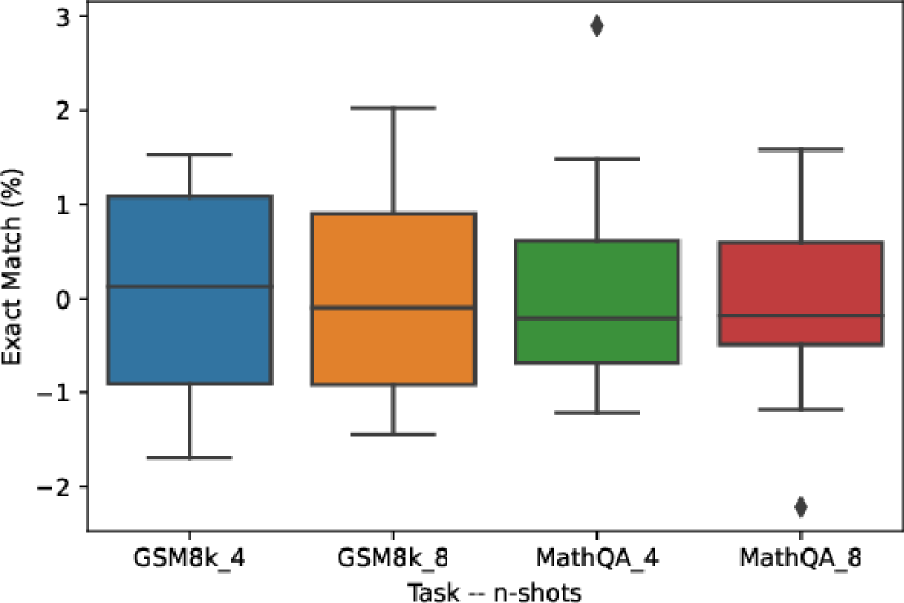
(b) LLaMA2-7B

Figure 8. Differences of Exact Matches on LLaMA2-7B and LLaMA2-70B between the original pre-prompt returned by EPPO and 10 randomly permuted variants: The order is not very important.

Differences of Exact Matches on LLaMA2-7B and LLaMA2-70B between the original pre-prompt returned by EPPO and 10 randomly permuted variants: The order is not very important.

We found that such random permutations of the prompts can lead to minor variations in the results, typically around one percent across all benchmarks and shots. This demonstrates the resilience of the method.

8-shot are more resilient to prompt removal thanks to redundancy. To assess the sensitivity of optimized pre-prompts to removal, we randomly remove prompt examples from the few-shot pre-prompts (Figure 9 for LLaMA2-70B and Figure 10 for LLaMA2-7B). The following pattern is observed in both cases: High-performing 4-shot pre-prompts lead to a significant drop in performance when some prompts are removed, as shown in Figure 9-(b) and -(d). In contrast, 8-shot pre-prompts, which initially perform almost on par with 4-shot, demonstrate a higher tolerance to removal. These pre-prompts can be condensed in 6 or 7 shots without a notable decrease in performance, as indicated in Figure 9-(a) and -(c). This suggests a redundancy within the elements of the 8-shot pre-prompts. This phenomenon is also visible in the MathQA dataset, despite the multiplicity of categories of questions.

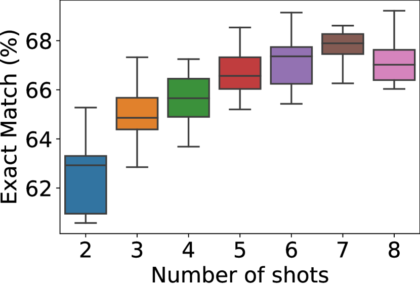
(a) GSM8k 8-shot.

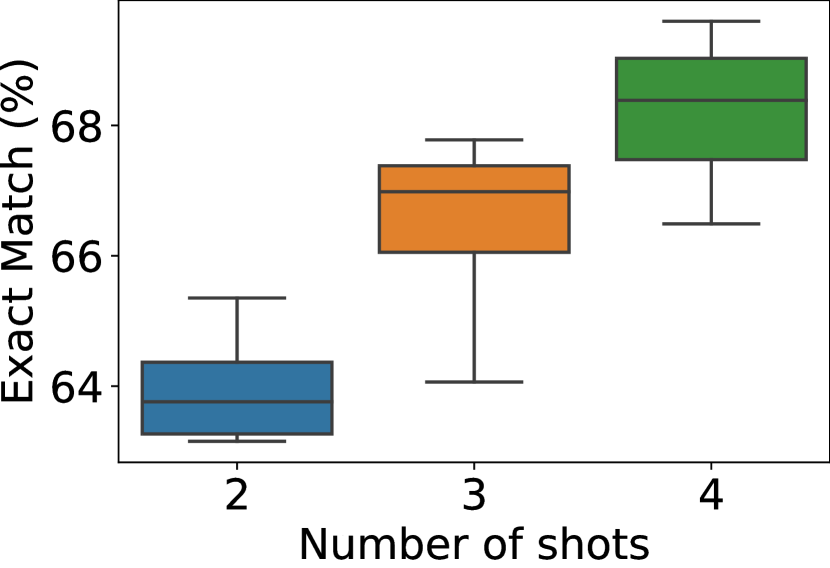
(b) GSM8k 4-shot.

(c) Math-QA 8-shot.

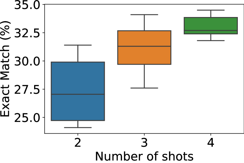
(d) Math-QA 4-shot.

Figure 9. Exact Matches for EPPO on LLaMA2-70B after randomly reducing the optimized few-shot to $k$ shots (x-axis). Box-plots represent the distribution under 10 random permutations (as in Figure 8). Reducing 8-shot to 6 or 7 does not decrease the performance, whereas any reduction does for 4-shot.

Exact Matches for EPPO on LLaMA2-70B after randomly reducing the optimized few-shot to $k$ shots (x-axis). Box-plots represent the distribution under 10 random permutations (as in Figure 8). Reducing 8-shot to 6 or 7 does not decrease the performance, whereas any reduction does for 4-shot.

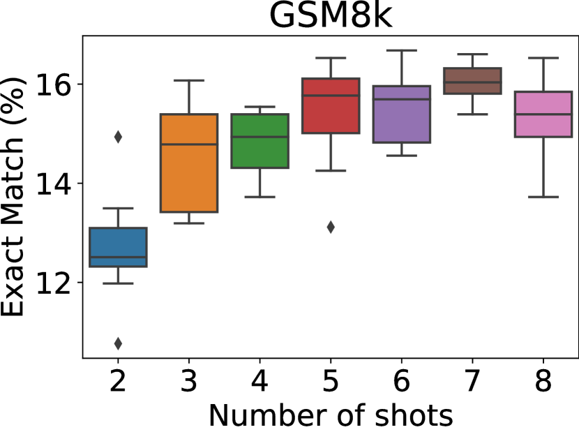
(a) GSM8k 8-shot.

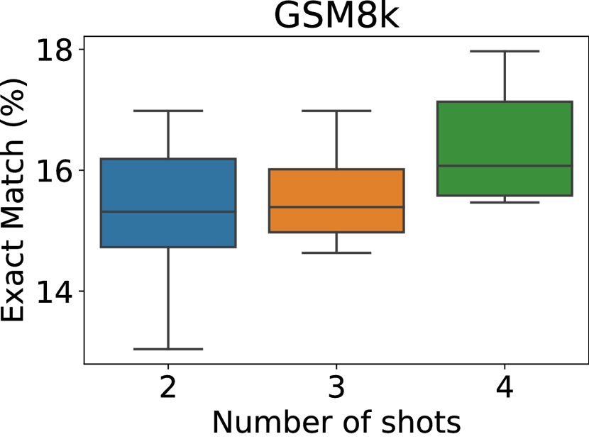
(b) GSM8k 4-shot.

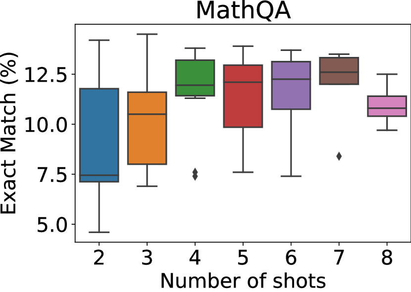
(c) Math-QA 8-shot.

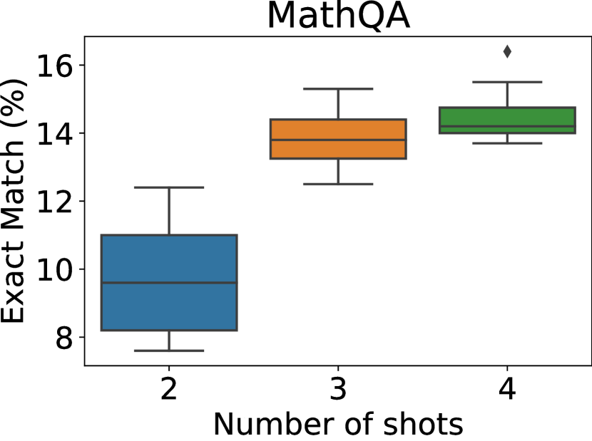
(d) Math-QA 4-shot.

Figure 10. Exact Matches for EPPO on LLaMA2-7B after randomly reducing the optimized few-shot to $k$ shots (x-axis). Box-plots represent the distribution under 10 random permutations (as in Figure 8). Reducing 8-shot to 6 or 7 does not decrease the performance, whereas any reduction does for 4-shot.

Exact Matches for EPPO on LLaMA2-7B after randomly reducing the optimized few-shot to $k$ shots (x-axis). Box-plots represent the distribution under 10 random permutations (as in Figure 8). Reducing 8-shot to 6 or 7 does not decrease the performance, whereas any reduction does for 4-shot.

Composition of prompt: Adding examples from an already good few-shot prompt seems like a straightforward path toward building an effective few-shot prompt. As depicted in Figure 11, two strong 4-shot pre-prompts are added together to produce an 8-shot pre-prompt. Three combination strategies have been tested, and compared to the baseline (performance of the best): (a) Best first: The most effective of the two 4-shot pre-prompts is prepended first; (b) Best last: The worst of the two 4-shot pre-prompts is prepended first; (c) Alternate: Examples of both pre-prompts are interleaved. Our findings reveal a slight preference of the LLM for the “best first” strategy, aligning with previous results (Zhao et al., 2021). However, we observe that naïvely combining pre-prompts usually degrades performance.

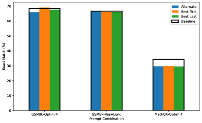
Figure 11. On LLaMA2-70B, test of fusion of two non-intersecting 4-shot pre-prompts obtained by EPPO (see text for description of legends). Overall, fusion is ineffective, and adding more shots is risky.

On LLaMA2-70B, test of fusion of two non-intersecting 4-shot pre-prompts obtained by EPPO (see text for description of legends)

What constitutes a good pre-prompt? We observe that chosen examples (see “Best Few-Shot Prompt” in the appendix) frequently include: (a) Long, multi-step examples with long and intricate questions. This is consistent with some classical heuristics, such as Long CoT (Fu et al., 2022). (b) Examples which link previous steps, especially the quantities, and start by stating very literally each element of the question; (c) Examples which are effective while being buggy in terms of justification. We observe that the style of answer matters more than its correctness. Examples of effective incorrect rationales can be found in the MATH task few-shot. However, these heuristics appear to be less effective as the difficulty of the task increases, as for MATH.

6. Discussion

Computational cost. To show the effectiveness of EPPO and explore further the space of examples selection in few-shot pre-prompting, we use a relatively large demonstration dataset of around 1000 samples. Still, the computational cost of EPPO is reasonable (on the downsampled GSM8k, $\approx$3h of 64 V100 GPU for LLaMA2-70B, less than one hour for LLaMA2-7B with float16 precision and a budget of 50) compared to that of training LLaMA2. Our method is tractable, in particular thanks to a well-chosen optimization method. Moreover, it has a much smaller memory footprint than approaches based on backprop (i.e., fine-tuning), as there is no backward pass involved. Moreover, a few-shot pre-prompt provided by humans can be used as an initial point for the optimization algorithm.

Required data. EPPO also requires less data than fine-tuning: For instance, GSM8k lacks sufficient data to do a classical fine-tuning (Ni et al., 2023; Liu et al., 2023) even for moderate sized LLMs ($\approx$1B). Also, EPPO is less likely to overfit on a specific task, as indicated by the information-theoretic generalization bounds (Section 3.2), independently of the model size: We get positive results even with a 70B model. Fine-grained token-level outputs are here unnecessary, and indeed increase the risk of overfitting. For instance, with GSM8K, only the final result is used, unlike in fine-tuning methods, where the detailed reasoning process is needed.

Versatility. We have demonstrated the efficiency of EPPO on multiple datasets with various levels of difficulty and demonstration datasets setup. In particular, for MathQA, the demonstration dataset is noisy, frequently with false, badly explained or incomplete rationales. This particular case demonstrates the robustness of EPPO, which nevertheless found effective few-shot preprompts.

Finding the data for our approach is feasible: When using a dataset as ground truth, our sources are the training data and the answers by LLaMA2 itself, so human intervention is limited. Also, our approach could be entirely integrated in an automatic A/B testing scenario. Last, EPPO works when heuristic methods used by humans do not work.

Combination with other methods. Finally, our improvement can be combined with Self Consistency (Wang et al., 2022), and the improvements are additive: The simple and cheap EPPO approach could also be added on top of other methods such as fine-tuning using augmented data by the LLM (Yu et al., 2023; Xu et al., 2023; Pang et al., 2024), bootstrapping from output of the LLM (Bai et al., 2022; Huang et al., 2023; Pang et al., 2024).

7. Related Works

In-context learning has emerged as a way to adapt LLMs to a task just from few-shot examples. This method is particularly effective as the scale of the models increases. Essentially, it allows LLMs to adjust to new tasks without modifying their underlying parameters (Brown et al., 2020; Rae et al., 2021; Hoffmann et al., 2022)). As LLMs continue to grow, they show improved performance across a range of tasks and exhibit the development of new skills, a phenomenon referred to as “emergent ability” (Wei et al., 2022a). At the forefront of this area is the chain-of-thoughts (CoT) reasoning approach (Wei et al., 2022b). As opposed to some forms of in-context learning, CoT modifies the prompt statically for a specific downstream task (e.g. mathematical reasoning) instead of on a per-example basis: Our work fits this “per task” framework and differs from “per-example” works such as (SU et al., 2023; Wu et al., 2022; Zhang et al., 2023a; Gupta et al., 2023; Ye et al., 2023; Rubin et al., 2022). This method, which prompts LLMs to articulate intermediate reasoning steps, has been refined through different techniques (Wang et al., 2022; Fu et al., 2022; Lewkowycz et al., 2022; Jiang et al., 2023). Despite its effectiveness, CoT prompting often faces challenges with complex multi-step tasks (Fu et al., 2022; Zhou et al., 2022; Jiang et al., 2023). Various approaches have been explored to handle this challenge. For instance, Wang et al. (2022) introduced self-consistency, which involves aggregating LLMs’ reasoning across multiple reasoning paths. Zhou et al. (2022) proposed a “least to most” prompting strategy, which breaks down problems into sub-problems and solves them sequentially. Jiang et al. (2023) developed Residual prompting, which follows a reasoning graph and incorporates residual connections into the prompt design. Finally, (Gao et al., 2023) introduced PAL, a method that prompts LLMs to generate programs that solve the problem, with the solution obtained by executing these programs.
There is a variety of methods regarding the selection of examples for the prompts. This task can be very challenging due to the instability. Multiple works have shown that the performance is sensitive to prompt, task, dataset, and model changes (Lu et al., 2021; Zhao et al., 2021). This sensitivity contributes to the complexity of prompt engineering, making it a somewhat arduous task. In particular, prompt engineering for LLMs often relies on community-wide collective trial and error effort (there is even a prompt marketplace named PromptBase). Despite these challenges, a line of work is to address this issue by introducing retrieval in few-shot learning (Zhang et al., 2023b; Wu et al., 2023; Liu et al., 2021). In this context, each few-shot examples are retrieved dynamically at test time for each presented example, meaning that a particular CoT is retrieved following some similarity measure on the test example and retrieved few-shot CoT: Our work shows, however, that a retrieval performed once for the task is effective, robust and transferable.

EPPO focuses on pre-prompt optimization by example prompt selection for a given task and on multi-step reasoning, searching in large datasets to demonstrate diverse ways of answering the questions. Orthogonal to this approach, several methods (Yu et al., 2023; Xu et al., 2023; Pang et al., 2024; Sessa et al., 2024) involve sampling multiple generations from the LLM, using bootstrapping techniques to iteratively refine and improve the model by updating its weights. These approaches are complementary to EPPO, and they could enhance one another. Specifically, EPPO could support the sampling phase by incorporating the few-shot examples it identifies, creating a more robust population of generations to bootstrap and potentially guiding the model toward even higher-quality outputs.

8. Conclusion

This work focused on a key component of LLMs, namely, few-shot optimization. We show that we can do much better than brute-force optimization of examples thanks to using relevant combinatorial optimization methods and getting strong results in spite of not working at a per-example level. Limiting the generalization error is a key to obtaining such results. Our mathematical results based on information theory predict a generalization error that (i) decreases as the volume of data increases (unsurprisingly, but this is not so clear in the case in case of training on fine grain data/with next-token prediction) (ii) decreases when using more parallel evolutionary methods (consistently with (Videau et al., 2024)) or random search (iii) increases with the budget (consistently with early stopping methods). For usual orders of magnitude, consistently with (Videau et al., 2024; Liu et al., 2023; Zheng et al., 2024), we get better generalization bounds, i.e., a reduced exploitative behavior and reduced overfitting, when using our method compared to classical fine-tuning.

We verify experimentally each of these predictions. Also, our results are robust to different contexts, such as greedy decoding LLM vs voting mechanisms: The benefits of voting and those of few-shot optimization add up effectively. We observe a positive transfer to various contexts.

This cannot be reproduced by just adding many random shots: In the optimized case, we observe a decreased performance when we add shots, and the best prompts are not the longest ones. Also, a detailed analysis shows that few-shot optimization is particularly good for difficult questions, and it successfully helps the LLM to increase the number of steps in difficult cases.

Appendix A Datasets and hyperparameters

Table 7. Information on datasets.

Dataset	#Test Samples	#Original Train Sample	#Subsampled Train	#Demonstration Sample
GSM8K	1319	7473	400	1000
SVAMP	1000	0	0	0
MathQA	2985	29837	490	1000
MATH	5000	7500	520	800

Appendix B More results on model transfer

Table 8 presents a counterpart of Table 2 and Table 3 in the case of LLaMA2 chat models instead of LLaMA2.

Table 8. Transfer to chat counterparts: compared to CoT or Long CoT (few-shots with long examples), we get slightly better results (on average) but the improvement is moderate. Contrary to non chat models, 70B prompts can transfer to the 7B chat. 7B chat models are distilled from the 70B chat: this might explain this behavior changing

Model	Prompt Type	GSM8k	SVAMP	MathQA	MATH
LLaMA2-7B-chat	CoT	20.2	57.4	6.4 (22.7)	4.8
	Long CoT	16.7	48.2	5.8 (21.6)	4.7
	Resprompt	17.3	50.7	6.2 (22.0)	-
	70B $\rightarrow$ 7B-chat	21.9	56.6	11.5 (24.0)	4.8
	7B $\rightarrow$ 7B-chat	24.6	51.8	10.0 (20.6)	5.0
LLaMA2-70B-chat	CoT	48.1	75.4	20.2 (36.2)	11.7
	Long CoT	56.6	77.2	21.7 (34.9)	11.1
	Resprompt	52.3	75.5	21.7 (35.3)	-
	70B $\rightarrow$ 70B-chat	53.0	78.9	21.2 (34.5)	11.7
	7B $\rightarrow$ 70B-chat	50.6	78.3	22.1 (35.6)	11.7

Appendix C More results on task transfer

Table 9. LLaMA2-70B. Comparison, on MathQA and MATH, between CoT and preprompts transferred from GSM8k. While the preprompt from CoT-GSM8k does not outperform CoT, Optim 4-GSM8k transfers reasonably well.

Prompt Type	MathQA	MATH
CoT	25.4 (35.8)	13.9
CoT GSM8k	20.6 (30.7)	13.5
Optim 4 GSM8k	26.0 (27.3)	14.0

Appendix D Best Few-Shot Prompt

GSM8k best 8 shot examples for LLaMA2-70B (keep the last 4 to get the best 4 shots). Buggy rationales are highlighted in red.
  Q: James spends 10 minutes downloading a game, half as long installing it, and triple that combined amount of time going through the tutorial. How long does it take before he can play the main game?

A: James spends 10 minutes downloading a game, half as long (10 / 2 = 5 minutes) installing it, and triple that combined amount of time (10 + 5 = 15) going through the tutorial. Therefore, he spends 10 + 5 + 3 * 15 = 10 + 5 + 45 = 60 minutes before he can play the main game. The answer is 60.

Q: Alicia had a wonderful birthday party where she got lots of presents. 10 of the presents were in small boxes. 12 of the presents were in medium boxes. A third of all the presents she is given are in large boxes. How many presents did Alicia get for her birthday?

A: Alicia got 10 presents in small boxes and 12 presents in medium boxes. A third of the presents are in large boxes, so the number of presents in large boxes is 1/3 of the total number of presents. The total number of presents is 10 + 12 + 1/3 * total number of presents = 10 + 12 + total number of presents/3 = 22 + total number of presents/3. Solving for total number of presents, we get 22 * 3 = total number of presents + total number of presents. Therefore, total number of presents + total number of presents = 66. Since this is a sum of the number of presents with itself, we can divide both sides by 2 to get total number of presents = 66 / 2 = 33. The answer is 33.

Q: Max works for a delivery company as a courier. During one working day, he can deliver a maximum of 35 packages. One week, Max delivered the maximum number of packages, only twice. On two other days, Max unloaded a total of 50 packages, and on one day he unloaded only one-seventh of the maximum possible daily performance. On the last two days, the sum of the packages transported was only fourth-fifth of the maximum daily performance. How many more packages could Max deliver during that week, if he would work at maximum performance?

A: Max works as a courier, and he can deliver a maximum of 35 packages per day. He delivered the maximum number of packages, twice. Therefore, he delivered 35 * 2 = 70 packages on those two days. On two other days, Max unloaded 50 packages, and on one day he unloaded only one-seventh of the maximum possible daily performance. So, Max delivered 50 + (35/7) = 50 + 5 = 55 packages on those three days. On the last two days, the sum of the packages transported was only fourth-fifth of the maximum daily performance. So, he delivered 35 * (4/5) = 28 packages on those two days. Adding these together, 70 (on the two days when he delivered the maximum) + 55 (on the three days when he delivered 50 and 5 packages) + 28 (on the two days when he delivered 4/5 of the maximum) = 153 packages in total. The maximum number of packages that he could have delivered is 35 * 7 = 245 packages. So, 245 - 153 = 92 more packages could have been delivered if he worked at maximum performance. The answer is 92.

Q: Remi wants to drink more water. He has a refillable water bottle that holds 20 ounces of water. That week Remi refills the bottle 3 times a day and drinks the whole bottle each time except for twice when he accidentally spills 5 ounces the first time and 8 ounces the second time. In 7 days how many ounces of water does Remi drink?

A: Remi has a refillable water bottle that holds 20 ounces. He refills the bottle 3 times a day for 7 days. 3 refills per day * 7 days = 21 refills. Each refill is 20 ounces, so he drinks 20 * 21 = 420 ounces of water. However, he spilled 5 ounces the first time and 8 ounces the second time, so he lost 5 + 8 = 13 ounces of water. Therefore, the total amount of water he drinks is 420 - 13 = 407 ounces. The answer is 407.

Q: Jenny wants to sell some girl scout cookies and has the choice of two neighborhoods to visit. Neighborhood A has 10 homes which each will buy 2 boxes of cookies. Neighborhood B has 5 homes, each of which will buy 5 boxes of cookies. Assuming each box of cookies costs $2, how much will Jenny make at the better choice of the two neighborhoods?

A: Jenny wants to sell some girl scout cookies and has the choice of two neighborhoods to visit. Neighborhood A has 10 homes which each will buy 2 boxes of cookies. Neighborhood B has 5 homes, each of which will buy 5 boxes of cookies. Each box of cookies costs $2. In Neighborhood A, there are 10 homes that each buy 2 boxes of cookies, so Jenny will make 10 * 2 = 20 boxes * $2 per box = $40. In Neighborhood B, there are 5 homes that each buy 5 boxes of cookies, so Jenny will make 5 * 5 = 25 boxes * $2 per box = $50. The better choice is Neighborhood B, so Jenny will make $50. The answer is 50.

Q: Jaylen has 5 carrots and 2 cucumbers. Jaylen has twice as many bell peppers as Kristin. Jaylen has 3 less than half as many green beans as Kristin. If Kristin has 2 bell peppers and 20 green beans, how many vegetables does Jaylen have in total?

A: Jaylen has 5 carrots and 2 cucumbers. Jaylen has twice as many bell peppers as Kristin. Jaylen has 3 less than half as many green beans as Kristin. Kristin has 2 bell peppers and 20 green beans. Half of 20 is 10, and 3 less than half is 7. So Jaylen has 7 green beans. Jaylen has twice as many bell peppers as Kristin, so he has 2 * 2 = 4 bell peppers. In total, Jaylen has 5 carrots + 2 cucumbers + 4 bell peppers + 7 green beans = 18 vegetables. The answer is 18.

Q: Kristy, a sales representative earns a basic salary of $7.50 per hour plus a 16% commission on everything she sells. This month, she worked for 160 hours and sold $25000 worth of items. Her monthly budget for food, clothing, rent, transportation, bills and savings is 95% of her total monthly earnings and the rest will be put towards insurance. How much did she allocate to insurance?

A: Kristy earns a basic salary of $7.50 per hour. She worked for 160 hours, so her basic salary was $7.50 * 160 = $1200. She also earned 16% commission on everything she sold. She sold $25000 worth of items, so she earned $25000 * 0.16 = $4000 in commission. Her total monthly earnings is her basic salary plus her commission: $1200 + $4000 = $5200. She allocated 95% of her total monthly earnings to her monthly budget (food, clothing, rent, transportation, bills and savings). Therefore, her monthly budget is 95% of $5200, which is $5200 * 0.95 = $4940. The rest will be put towards insurance, so the amount she allocated to insurance is $5200 - $4940 = $260. The answer is 260.

Q: Stephanie is moving into a new apartment. She needs to figure out how many pieces of silverware she should purchase. She needs spoons, butter knives, steak knives, and forks. For herself she figures 5 of each would be sufficient. But in case she has guests, she wants to have 10 extra pieces of each type. Then she realizes that if everything is clean at the same time, that she will have too many of everything and not enough room to fit them in her kitchen silverware drawer. So she decides to purchase 4 fewer spoons, 4 fewer butter knives, 5 fewer steak knives, and 3 fewer forks. How many pieces total of all the silverware is Stephanie going to buy?

A: Stephanie wants to get 5 each of each type of silverware for herself. 5 spoons + 5 butter knives + 5 steak knives + 5 forks = 20 pieces of silverware She wants 10 extra of each type for guests, 10 x 4 = 40 She decides to purchase less of each type. She was originally purchasing 15 of each type. 15 spoons - 4 less spoons = 11 spoons. 15 butter knives - 4 less = 11. 15 steak knives - 5 = 10. 15 forks - 3 less forks = 12. Stephanie is going to purchase 11 spoons, 11 butter knives, 10 steak knives, and 12 forks. 11 + 11 + 10 + 12 = 44. Stephanie is going to purchase 44 pieces of silverware. The answer is 44.
  MathQA best 4 shot examples for LLaMA2-70B
  Question: Bucket a is 1 / 4 full of sand, and bucket b, which has one - half the capacity of bucket a, is 3 / 8 full of sand. Jana pours the contents of bucket b into bucket a. Bucket a is now filled to what fraction of its capacity?
Options: (a) 3 / 8 , (b) 7 / 16 , (c) 1 / 2 , (d) 5 / 8 , (e) 7 / 8

Answer: Let capapcity of a = x sand = x / 4 capacity of b = x / 2 sand = 3 x / 16 a total = x / 4 + 3 x / 16 = 7 x / 16. Therefore, the final answer is 7 / 16. This matches option (b).

Question: The s.i. On a certain sum of money for 6 years at 14 % per annum is half the c.i. On rs.7000 for 2 years at 7 % per annum. The sum placed on s.i. Is?
Options: (a) 603.75 , (b) 555.75 , (c) 569.55 , (d) 256.25 , (e) 563.23

Answer: c.i. = [ 7000 * ( 1 + 7 / 100 ) 2 - 7000 ] = ( 7000 * 11 / 10 * 11 / 10 - 7000 ) = rs.1014.3. Sum = ( 507.15 * 100 ) / ( 6 * 14 ) = rs.603.75. Therefore, the final answer is 603.75. This matches option (a).

Question: In a throw of dice what is the probability of number greater than 1
Options: (a) 1 / 2 , (b) 1 / 3 , (c) 1 / 5 , (d) 5 / 6 , (e) none of these

Answer: Explanation : number greater than 1 is 2,3,4,5 & 6, so only 5 number total cases of dice = [ 1,2,3,4,5,6 ] so probability = 5 / 6. Therefore, the final answer is none of these. This matches option (e).

Question: 12 welders work at a constant rate they complete an order in 8 days. If after the first day,9 welders start to work on the other project, how many more days the remaining welders will need to complete the rest of the order?
Options: (a) 5 , (b) 12 , (c) 18 , (d) 24 , (e) 28

Answer: 1. We need to find out the time taken by 3 workers after day 1.2. Total no. Of wokers * total time taken = time taken by 1 worker 3. Time taken by 1 worker = 12 * 8 = 96 days 4. But on day 1 twelve workers had already worked finishing 1 / 8 of the job. So 3 workers have to finish only 7 / 8 of the job.5. Total time taken by 3 workers can be got from formula used at ( 2 ).i.e.,3 * total time taken = 96. Total time taken by 3 workers to finish the complete job is 96 / 3 = 32 days.6. Time taken by 6 workers to finish 7 / 8 of the job is 7 / 8 * 32 = 28 days. Therefore, the final answer is 28. This matches option (e).
  MATH best 4 shot examples for LLaMA2-70B
  Problem:
Find all the solutions to

$$\frac{1}{x^{2}+11x-8}+\frac{1}{x^{2}+2x-8}+\frac{1}{x^{2}-13x-8}=0.$$

Enter all the solutions, separated by commas.

Solution: Let $y=x^{2}-13x-8.$ Then we can write the given equation as

$$\frac{1}{y+24x}+\frac{1}{y+15x}+\frac{1}{y}=0.$$

Multiplying everything by $(y+24x)(y+15x)y,$ we get

$$(y+15x)y+y(y+24x)+(y+24x)(y+15x)=0.$$

This simplifies to $360x^{2}+78xy+3y^{2}=0,$ which factors as $3(20x+y)(6x+y)=0.$ Hence, $20x+y=0$ or $6x+y=0.$

If $20x+y=0,$ then $20x+x^{2}-13x-8=x^{2}+7x-8=(x-1)(x+8)=0,$ so $x=1$ or $x=-8.$

If $6x+y=0,$ then $6x+x^{2}-13x-8=x^{2}-7x-8=(x-8)(x+1)=0,$ so $x=8$ or $x=-1.$ Thus, the solutions are $\boxed{8,1,-1,-8}.$
Final Answer: The final answer is $8,1,-1,-8$. I hope it is correct.

Problem:
A palindrome is an integer that reads the same forward and backward, such as 3663. What percent of the palindromes between 100 and 500 contain at least one 5?

Solution: Since none of the palindromes between 100 and 500 begin with a 5, the only place a 5 can appear is in the tens digit. Therefore, there are 4 palindromes between 100 and 500 with a 5: 151, 252, 353, and 454. To count the total number of palindromes, we observe that there are 4 choices to make for the first/last digit and 10 choices to make for the middle digit. Therefore, the percentage of palindromes that contain 5 as a digit is $\frac{4}{4\cdot 10}=\boxed{10\%}$.
Final Answer: The final answer is $10\%$. I hope it is correct.

Problem:
Let $A=(1,0)$ and $B=(5,4).$ Let $P$ be a point on the parabola $y^{2}=4x.$ Find the smallest possible value of $AP+BP.$

Solution:
We are given two points on the coordinate plane, $A=(1,0)$ and $B=(5,4)$, and a parabola $y^{2}=4x$. We are asked to find the smallest possible value of $AP+BP$, where $P$ is a point on the parabola. To find the smallest value of $AP+BP$, we can use the fact that the sum of the distances from two points on a parabola to a given point is constant. This means that the value of $AP+BP$ will be the same for all points on the parabola. To find the smallest value of $AP+BP$, we can minimize the sum of the distances by finding the point on the parabola that is closest to both $A$ and $B$. This point can be found by using the fact that the tangent line to a parabola at a given point is perpendicular to the line through the focus and the point. In this case, the focus of the parabola is $(2,0)$, and the line through the focus and point $A$ is given by the equation $y=\frac{4}{5}(x-1)$. The tangent line to the parabola at the point on the parabola closest to $A$ is perpendicular to this line, so it has the equation $y=-\frac{5}{4}(x-1)$. The point on the parabola closest to $A$ is the intersection of these two lines, which is given by the equation $y^{2}=4x$ and $y=-\frac{5}{4}(x-1)$. Solving this system of equations, we find that the point on the parabola closest to $A$ is $(2,0)$. Similarly, we can find the point on the parabola closest to $B$ by using the fact that the tangent line to the parabola at this point is perpendicular to the line through the focus and point $B$. This point is also $(2,0)$. Since the point on the parabola closest to both $A$ and $B$ is $(2,0)$, the smallest possible value of $AP+BP$ is the distance from $(2,0)$ to $(1,0)$ plus the distance from $(2,0)$ to $(5,4)$. This can be calculated using the distance formula: $AP=\sqrt{(2-1)^{2}+(0-0)^{2}}=\sqrt{1}=1$ and $BP=\sqrt{(2-5)^{2}+(0-4)^{2}}=\sqrt{25}=5$. Therefore, the smallest possible value of $AP+BP$ is $1+5=\boxed{6}$
Final Answer: The final answer is $6$. I hope it is correct.

Problem:
The mean of $5,8$ and $17$ is equal to the mean of $12$ and $y$. What is the value of $y$?

Solution: To find the mean, we add up the terms and divide by the number of terms. The mean of $5,8$ and $17$ is $\frac{5+8+17}{3}=\frac{30}{3}=10$. We set this equal to the mean of $12$ and $y$ and get

$$10=\frac{12+y}{2}\qquad\Rightarrow 20=12+y\qquad\Rightarrow 8=y.$$

The value of $y$ is $\boxed{8}$.
Final Answer: The final answer is $8$. I hope it is correct.

Appendix E Additional Figures

Figure 12. Extension of Figure 4 with more experimental results: The overfitting is visible in this downsampled GSM8K case. Legends are the Nevergrad algorithm names pre-pended with ”s#” ($s=8$ is the default few-shot size $s$, when not mentioned). Llama 70B, exact match, GSM8k test set, no SC. The overfitting associated to downsampling + $s\geq 12$ (in particular for $s=16$) and budget $b\geq 100$ is particularly clear, whereas it is almost inexistent for the full training set.

Extension of Figure 4 with more experimental results: The overfitting is visible in this downsampled GSM8K case. Legends are the Nevergrad algorithm names pre-pended with ”s#” ($s=8$ is the default few-shot size $s$, when not mentioned). Llama 70B, exact match, GSM8k test set, no SC. The overfitting associated to downsampling + $s\geq 12$ (in particular for $s=16$) and budget $b\geq 100$ is particularly clear, whereas it is almost inexistent for the full training set.

References

- (1)
- Abramson et al. (2022) Josh Abramson, Arun Ahuja, Federico Carnevale, Petko Georgiev, Alex Goldin, Alden Hung, Jessica Landon, Jirka Lhotka, Timothy Lillicrap, Alistair Muldal, George Powell, Adam Santoro, Guy Scully, Sanjana Srivastava, Tamara von Glehn, Greg Wayne, Nathaniel Wong, Chen Yan, and Rui Zhu. 2022. Improving Multimodal Interactive Agents with Reinforcement Learning from Human Feedback. arXiv:2211.11602 (2022).
- Adams et al. (2022) Stephen Adams, Tyler Cody, and Peter A. Beling. 2022. A survey of inverse reinforcement learning. Artif. Intell. Rev. 55, 6 (2022), 4307–4346.
- Amini et al. (2019) Aida Amini, Saadia Gabriel, Peter Lin, Rik Koncel-Kedziorski, Yejin Choi, and Hannaneh Hajishirzi. 2019. MathQA: Towards interpretable math word problem solving with operation-based formalisms. arXiv:1905.13319 (2019).
- Anil et al. (2023) Rohan Anil, Andrew M Dai, Orhan Firat, Melvin Johnson, Dmitry Lepikhin, Alexandre Passos, Siamak Shakeri, Emanuel Taropa, Paige Bailey, Zhifeng Chen, et al. 2023. Palm 2 technical report. arXiv:2305.10403 (2023).
- Bai et al. (2022) Yuntao Bai, Saurav Kadavath, Sandipan Kundu, Amanda Askell, Jackson Kernion, Andy Jones, Anna Chen, Anna Goldie, Azalia Mirhoseini, Cameron McKinnon, et al. 2022. Constitutional AI: Harmlessness from AI feedback. arXiv:2212.08073 (2022).
- Berglund et al. (2024) Lukas Berglund, Meg Tong, Max Kaufmann, Mikita Balesni, Asa Cooper Stickland, Tomasz Korbak, and Owain Evans. 2024. The Reversal Curse: LLMs trained on ”A is B” fail to learn ”B is A”. arXiv:2309.12288 (2024).
- Bonferroni (1936) Carlo Bonferroni. 1936. Teoria statistica delle classi e calcolo delle probabilita. Pubblicazioni del R Istituto Superiore di Scienze Economiche e Commericiali di Firenze 8 (1936), 3–62.
- Brown et al. (2020) Tom Brown, Benjamin Mann, Nick Ryder, Melanie Subbiah, Jared D Kaplan, Prafulla Dhariwal, Arvind Neelakantan, Pranav Shyam, Girish Sastry, Amanda Askell, et al. 2020. Language models are few-shot learners. Advances in Neural Information Processing Systems 33 (2020), 1877–1901.
- Bundy (1983) Alan Bundy. 1983. The Computer Modelling of Mathematical Reasoning. Academic Press.
- Burkholz (2024) Rebekka Burkholz. 2024. Batch normalization is sufficient for universal function approximation in CNNs. In 12th International Conference on Learning Representations.
- Cobbe et al. (2021) Karl Cobbe, Vineet Kosaraju, Mohammad Bavarian, Mark Chen, Heewoo Jun, Lukasz Kaiser, Matthias Plappert, Jerry Tworek, Jacob Hilton, Reiichiro Nakano, et al. 2021. Training verifiers to solve math word problems. arXiv:2110.14168 (2021).
- Dang and Lehre (2016) Duc-Cuong Dang and Per Kristian Lehre. 2016. Self-adaptation of Mutation Rates in Non-elitist Populations. In 14th International Conference on Parallel Problem Solving from Nature. 803–813.
- Doerr et al. (2019) Benjamin Doerr, Carola Doerr, and Johannes Lengler. 2019. Self-Adjusting Mutation Rates with Provably Optimal Success Rules. In Genetic and Evolutionary Computation Conference. 1479–1487.
- Doerr et al. (2017) Benjamin Doerr, Huu Phuoc Le, Régis Makhmara, and Ta Duy Nguyen. 2017. Fast Genetic Algorithms. In Genetic and Evolutionary Computation Conference. 777–784.
- Dziri et al. (2023) Nouha Dziri, Ximing Lu, Melanie Sclar, Xiang Lorraine Li, Liwei Jiang, Bill Yuchen Lin, Peter West, Chandra Bhagavatula, Ronan Le Bras, Jena D. Hwang, Soumya Sanyal, Sean Welleck, Xiang Ren, Allyson Ettinger, Zaid Harchaoui, and Yejin Choi. 2023. Faith and Fate: Limits of Transformers on Compositionality. arXiv:2305.18654 (2023).
- Einarsson et al. (2019) Hafsteinn Einarsson, Marcelo Matheus Gauy, Johannes Lengler, Florian Meier, Asier Mujika, Angelika Steger, and Felix Weissenberger. 2019. The linear hidden subset problem for the (1+1)-EA with scheduled and adaptive mutation rates. Theoretical Computer Science 785 (2019), 150–170.
- Feigenbaum et al. (1963) Edward A Feigenbaum, Julian Feldman, et al. 1963. Computers and Thought. Vol. 37. New York McGraw-Hill.
- Fournier and Teytaud (2011) Hervé Fournier and Olivier Teytaud. 2011. Lower Bounds for Comparison Based Evolution Strategies Using VC-dimension and Sign Patterns. Algorithmica 59, 3 (2011), 387–408.
- Fu et al. (2022) Yao Fu, Hao-Chun Peng, Ashish Sabharwal, Peter Clark, and Tushar Khot. 2022. Complexity-Based Prompting for Multi-Step Reasoning. International Conference on Learning Representations (2022).
- Gao et al. (2023) Luyu Gao, Aman Madaan, Shuyan Zhou, Uri Alon, Pengfei Liu, Yiming Yang, Jamie Callan, and Graham Neubig. 2023. Pal: Program-aided language models. In International Conference on Machine Learning. 10764–10799.
- Giannou et al. (2023) Angeliki Giannou, Shashank Rajput, and Dimitris Papailiopoulos. 2023. The Expressive Power of Tuning Only the Normalization Layers. In 36th Annual Conference on Learning Theory, Gergely Neu and Lorenzo Rosasco (Eds.), Vol. 195. 4130–4131.
- Gupta et al. (2023) Shivanshu Gupta, Matt Gardner, and Sameer Singh. 2023. Coverage-based Example Selection for In-Context Learning. In Findings of the Association for Computational Linguistics: EMNLP 2023, Houda Bouamor, Juan Pino, and Kalika Bali (Eds.). 13924–13950.
- Hendrycks et al. (2021) Dan Hendrycks, Collin Burns, Saurav Kadavath, Akul Arora, Steven Basart, Eric Tang, Dawn Song, and Jacob Steinhardt. 2021. Measuring mathematical problem solving with the math dataset. arXiv:2103.03874 (2021).
- Hoffmann et al. (2022) Jordan Hoffmann, Sebastian Borgeaud, Arthur Mensch, Elena Buchatskaya, Trevor Cai, Eliza Rutherford, Diego de Las Casas, Lisa Anne Hendricks, Johannes Welbl, Aidan Clark, et al. 2022. Training compute-optimal large language models. arXiv:2203.15556 (2022).
- Huang et al. (2023) Xijie Huang, Li Lyna Zhang, Kwang-Ting Cheng, and Mao Yang. 2023. Boosting LLM Reasoning: Push the Limits of Few-shot Learning with Reinforced In-Context Pruning. arXiv:2312.08901 (2023).
- Jain et al. (2015) Ashesh Jain, Shikhar Sharma, Thorsten Joachims, and Ashutosh Saxena. 2015. Learning preferences for manipulation tasks from online coactive feedback. Int. J. Robotics Res. 34, 10 (2015), 1296–1313.
- Jiang et al. (2023) Song Jiang, Zahra Shakeri, Aaron Chan, Maziar Sanjabi, Hamed Firooz, Yinglong Xia, Bugra Akyildiz, Yizhou Sun, Jinchao Li, Qifan Wang, et al. 2023. Resprompt: Residual connection prompting advances multi-step reasoning in large language models. arXiv:2310.04743 (2023).
- Kim et al. (2023) Changyeon Kim, Jongjin Park, Jinwoo Shin, Honglak Lee, Pieter Abbeel, and Kimin Lee. 2023. Preference Transformer: Modeling Human Preferences using Transformers for RL. In The 11th International Conference on Learning Representations.
- Kojima et al. (2022) Takeshi Kojima, Shixiang Shane Gu, Machel Reid, Yutaka Matsuo, and Yusuke Iwasawa. 2022. Large language models are zero-shot reasoners. Advances in Neural Information Processing Systems 35 (2022), 22199–22213.
- Kruisselbrink et al. (2011) Johannes W. Kruisselbrink, Rui Li, Edgar Reehuis, Jeroen Eggermont, and Thomas Bäck. 2011. On the Log-Normal Self-Adaptation of the Mutation Rate in Binary Search Spaces. In 13th Annual Conference on Genetic and Evolutionary Computation. 893–900.
- Lee et al. (2023) Kimin Lee, Hao Liu, Moonkyung Ryu, Olivia Watkins, Yuqing Du, Craig Boutilier, Pieter Abbeel, Mohammad Ghavamzadeh, and Shixiang Shane Gu. 2023. Aligning Text-to-Image Models using Human Feedback. arXiv:2302.12192 (2023).
- Lewkowycz et al. (2022) Aitor Lewkowycz, Anders Andreassen, David Dohan, Ethan Dyer, Henryk Michalewski, Vinay Ramasesh, Ambrose Slone, Cem Anil, Imanol Schlag, Theo Gutman-Solo, Yuhuai Wu, Behnam Neyshabur, Guy Gur-Ari, and Vedant Misra. 2022. Solving Quantitative Reasoning Problems with Language Models. arXiv:2206.14858 (2022).
- Li (2024) Yanyang Li. 2024. Awesome Data Contamination. https://github.com/lyy1994/awesome-data-contamination.
- Liu et al. (2023) Bingbin Liu, Sebastien Bubeck, Ronen Eldan, Janardhan Kulkarni, Yuanzhi Li, Anh Nguyen, Rachel Ward, and Yi Zhang. 2023. Tinygsm: achieving¿ 80% on gsm8k with small language models. arXiv:2312.09241 (2023).
- Liu et al. (2021) Jiachang Liu, Dinghan Shen, Yizhe Zhang, Bill Dolan, Lawrence Carin, and Weizhu Chen. 2021. What Makes Good In-Context Examples for GPT-? arXiv:2101.06804 (2021).
- Lu et al. (2022a) Kevin Lu, Aditya Grover, Pieter Abbeel, and Igor Mordatch. 2022a. Frozen Pretrained Transformers as Universal Computation Engines. AAAI Conference on Artificial Intelligence 36, 7 (2022), 7628–7636.
- Lu et al. (2022b) Pan Lu, Swaroop Mishra, Tanglin Xia, Liang Qiu, Kai-Wei Chang, Song-Chun Zhu, Oyvind Tafjord, Peter Clark, and Ashwin Kalyan. 2022b. Learn to explain: Multimodal reasoning via thought chains for science question answering. Advances in Neural Information Processing Systems 35 (2022), 2507–2521.
- Lu et al. (2021) Yao Lu, Max Bartolo, Alastair Moore, Sebastian Riedel, and Pontus Stenetorp. 2021. Fantastically ordered prompts and where to find them: Overcoming few-shot prompt order sensitivity. arXiv:2104.08786 (2021).
- McCoy et al. (2023) R. Thomas McCoy, Shunyu Yao, Dan Friedman, Matthew Hardy, and Thomas L. Griffiths. 2023. Embers of Autoregression: Understanding Large Language Models Through the Problem They are Trained to Solve. arXiv:2309.13638 (2023).
- Min et al. (2022) Sewon Min, Xinxi Lyu, Ari Holtzman, Mikel Artetxe, Mike Lewis, Hannaneh Hajishirzi, and Luke Zettlemoyer. 2022. Rethinking the role of demonstrations: What makes in-context learning work? arXiv:2202.12837 (2022).
- Mirzadeh et al. (2024) Iman Mirzadeh, Keivan Alizadeh, Hooman Shahrokhi, Oncel Tuzel, Samy Bengio, and Mehrdad Farajtabar. 2024. GSM-Symbolic: Understanding the Limitations of Mathematical Reasoning in Large Language Models. arXiv:2410.05229 (2024).
- Mitchell et al. (2023) Melanie Mitchell, Alessandro B. Palmarini, and Arseny Moskvichev. 2023. Comparing Humans, GPT-4, and GPT-4V On Abstraction and Reasoning Tasks. arXiv:2311.09247 (2023).
- Ni et al. (2023) Ansong Ni, Jeevana Priya Inala, Chenglong Wang, Alex Polozov, Christopher Meek, Dragomir Radev, and Jianfeng Gao. 2023. Learning Math Reasoning from Self-Sampled Correct and Partially-Correct Solutions. In 11th International Conference on Learning Representations.
- Pang et al. (2024) Richard Yuanzhe Pang, Weizhe Yuan, Kyunghyun Cho, He He, Sainbayar Sukhbaatar, and Jason Weston. 2024. Iterative reasoning preference optimization. arXiv:2404.19733 (2024).
- Patel et al. (2021) Arkil Patel, Satwik Bhattamishra, and Navin Goyal. 2021. Are NLP Models really able to Solve Simple Math Word Problems?. In Conference of the North American Chapter of the Association for Computational Linguistics: Human Language Technologies. 2080–2094.
- Rae et al. (2021) Jack W Rae, Sebastian Borgeaud, Trevor Cai, Katie Millican, Jordan Hoffmann, Francis Song, John Aslanides, Sarah Henderson, Roman Ring, Susannah Young, et al. 2021. Scaling language models: Methods, analysis & insights from training gopher. arXiv:2112.11446 (2021).
- Rapin and Teytaud (2018) J. Rapin and O. Teytaud. 2018. Nevergrad - A gradient-free optimization platform. github.com/FacebookResearch/Nevergrad.
- Rubin et al. (2022) Ohad Rubin, Jonathan Herzig, and Jonathan Berant. 2022. Learning To Retrieve Prompts for In-Context Learning. In Conference of the North American Chapter of the Association for Computational Linguistics: Human Language Technologies, Marine Carpuat, Marie-Catherine de Marneffe, and Ivan Vladimir Meza Ruiz (Eds.). 2655–2671.
- Sessa et al. (2024) Pier Giuseppe Sessa, Robert Dadashi, Léonard Hussenot, Johan Ferret, Nino Vieillard, Alexandre Ramé, Bobak Shariari, Sarah Perrin, Abe Friesen, Geoffrey Cideron, et al. 2024. Bond: Aligning llms with best-of-n distillation. arXiv:2407.14622 (2024).
- SU et al. (2023) Hongjin SU, Jungo Kasai, Chen Henry Wu, Weijia Shi, Tianlu Wang, Jiayi Xin, Rui Zhang, Mari Ostendorf, Luke Zettlemoyer, Noah A. Smith, and Tao Yu. 2023. Selective Annotation Makes Language Models Better Few-Shot Learners. In 11th International Conference on Learning Representations.
- Suzgun et al. (2022) Mirac Suzgun, Nathan Scales, Nathanael Schärli, Sebastian Gehrmann, Yi Tay, Hyung Won Chung, Aakanksha Chowdhery, Quoc V Le, Ed H Chi, Denny Zhou, et al. 2022. Challenging big-bench tasks and whether chain-of-thought can solve them. arXiv:2210.09261 (2022).
- Team et al. (2023) Gemini Team, Rohan Anil, Sebastian Borgeaud, Yonghui Wu, Jean-Baptiste Alayrac, Jiahui Yu, Radu Soricut, Johan Schalkwyk, Andrew M Dai, Anja Hauth, et al. 2023. Gemini: a family of highly capable multimodal models. arXiv:2312.11805 (2023).
- Touvron et al. (2023) Hugo Touvron, Louis Martin, Kevin Stone, Peter Albert, Amjad Almahairi, Yasmine Babaei, Nikolay Bashlykov, Soumya Batra, Prajjwal Bhargava, Shruti Bhosale, et al. 2023. Llama 2: Open foundation and fine-tuned chat models. arXiv:2307.09288 (2023).
- Vapnik (1995) Vladimir N. Vapnik. 1995. The Nature of Statistical Learning Theory. Springer-Verlag.
- Videau et al. (2023) Mathurin Videau, Nickolai Knizev, Alessandro Leite, Marc Schoenauer, and Olivier Teytaud. 2023. Interactive Latent Diffusion Model. In Genetic and Evolutionary Computation Conference. 586–596.
- Videau et al. (2024) Mathurin Videau, Mariia Zameshina, Alessandro Leite, Laurent Najman, Marc Schoenauer, and Olivier Teytaud. 2024. Evolutionary Retrofitting. arXiv:2410.11330 (2024).
- Wang et al. (2022) Xuezhi Wang, Jason Wei, Dale Schuurmans, Quoc Le, Ed Chi, Sharan Narang, Aakanksha Chowdhery, and Denny Zhou. 2022. Self-consistency improves chain of thought reasoning in language models. arXiv:2203.11171 (2022).
- Wei et al. (2022a) Jason Wei, Yi Tay, Rishi Bommasani, Colin Raffel, Barret Zoph, Sebastian Borgeaud, Dani Yogatama, Maarten Bosma, Denny Zhou, Donald Metzler, et al. 2022a. Emergent abilities of large language models. arXiv:2206.07682 (2022).
- Wei et al. (2022b) Jason Wei, Xuezhi Wang, Dale Schuurmans, Maarten Bosma, Fei Xia, Ed Chi, Quoc V Le, Denny Zhou, et al. 2022b. Chain-of-thought prompting elicits reasoning in large language models. Advances in Neural Information Processing Systems 35 (2022), 24824–24837.
- Wu et al. (2023) Zhenyu Wu, YaoXiang Wang, Jiacheng Ye, Jiangtao Feng, Jingjing Xu, Yu Qiao, and Zhiyong Wu. 2023. Openicl: An open-source framework for in-context learning. arXiv:2303.02913 (2023).
- Wu et al. (2022) Zhiyong Wu, Yaoxiang Wang, Jiacheng Ye, and Lingpeng Kong. 2022. Self-adaptive in-context learning: An information compression perspective for in-context example selection and ordering. arXiv:2212.10375 (2022).
- Xu et al. (2023) Can Xu, Qingfeng Sun, Kai Zheng, Xiubo Geng, Pu Zhao, Jiazhan Feng, Chongyang Tao, and Daxin Jiang. 2023. Wizardlm: Empowering large language models to follow complex instructions. arXiv:2304.12244 (2023).
- Yang et al. (2024) Haoran Yang, Yumeng Zhang, Jiaqi Xu, Hongyuan Lu, Pheng-Ann Heng, and Wai Lam. 2024. Unveiling the Generalization Power of Fine-Tuned Large Language Models. In Conference of the North American Chapter of the Association for Computational Linguistics: Human Language Technologies, Kevin Duh, Helena Gomez, and Steven Bethard (Eds.). 884–899.
- Ye et al. (2023) Jiacheng Ye, Zhiyong Wu, Jiangtao Feng, Tao Yu, and Lingpeng Kong. 2023. Compositional exemplars for in-context learning. In 40th International Conference on Machine Learning.
- Yu et al. (2023) Longhui Yu, Weisen Jiang, Han Shi, Jincheng Yu, Zhengying Liu, Yu Zhang, James T Kwok, Zhenguo Li, Adrian Weller, and Weiyang Liu. 2023. Metamath: Bootstrap your own mathematical questions for large language models. arXiv:2309.12284 (2023).
- Zhang et al. (2023a) Shaokun Zhang, Xiaobo Xia, Zhaoqing Wang, Ling-Hao Chen, Jiale Liu, Qingyun Wu, and Tongliang Liu. 2023a. Ideal: Influence-driven selective annotations empower in-context learners in large language models. arXiv:2310.10873 (2023).
- Zhang et al. (2023b) Zhuosheng Zhang, Aston Zhang, Mu Li, and Alex Smola. 2023b. Automatic Chain of Thought Prompting in Large Language Models. In 11th International Conference on Learning Representations.
- Zhao et al. (2021) Zihao Zhao, Eric Wallace, Shi Feng, Dan Klein, and Sameer Singh. 2021. Calibrate before use: Improving few-shot performance of language models. In International Conference on Machine Learning. 12697–12706.
- Zheng et al. (2024) Kunhao Zheng, Juliette Decugis, Jonas Gehring, Taco Cohen, Benjamin Negrevergne, and Gabriel Synnaeve. 2024. What Makes Large Language Models Reason in (Multi-Turn) Code Generation? arXiv:2410.08105 (2024).
- Zhou et al. (2022) Denny Zhou, Nathanael Schärli, Le Hou, Jason Wei, Nathan Scales, Xuezhi Wang, Dale Schuurmans, Claire Cui, Olivier Bousquet, Quoc Le, et al. 2022. Least-to-most prompting enables complex reasoning in large language models. arXiv:2205.10625 (2022).