Multi-cam Multi-map Visual Inertial Localization:
System, Validation and Dataset

Abstract

Map-based localization is crucial for the autonomous movement of robots as it provides real-time positional feedback. However, existing VINS and SLAM systems cannot be directly integrated into the robot’s control loop. Although VINS offers high-frequency position estimates, it suffers from drift in long-term operation. And the drift-free trajectory output by SLAM is post-processed with loop correction, which is non-causal. In practical control, it is impossible to update the current pose with future information. Furthermore, existing SLAM evaluation systems measure accuracy after aligning the entire trajectory, which overlooks the transformation error between the odometry start frame and the ground truth frame. To address these issues, we propose a multi-cam multi-map visual inertial localization system, which provides real-time, causal and drift-free position feedback to the robot control loop. Additionally, we analyze the error composition of map-based localization systems and propose a set of evaluation metric suitable for measuring causal localization performance. To validate our system, we design a multi-camera IMU hardware setup and collect a long-term challenging campus dataset. Experimental results demonstrate the higher real-time localization accuracy of the proposed system. To foster community development, both the system and the dataset have been made open source https://github.com/zoeylove/Multi-cam-Multi-map-VILO/tree/main.

I Introduction

Map-based visual-inertial localization (VILO) refers to obtaining real-time state estimates under a map frame by incorporating observations from pre-constructed maps. In practical applications, VILO is of great significance for autonomous robots. This is because, from a robot control perspective, VILO provides real-time, causal and drift-free feedback that can be integrated into the position control loop. Neither VINS (visual-inertial navigation system) nor SLAM (simultaneous localization and mapping) can meet this demand. Although VINS provides real-time pose estimation[1][2][3][4], it accumulates drift over time. SLAM eliminates drift after loop closure correction is performed. This means that the drift-free pose provided by SLAM has a long time lag, which is non-causal as a feedback for control. A typical application of VILO currently is the autonomous driving system based on HD (high definition) maps. However, this system relies on many predefined semantic elements, such as traffic lights and lane markings, which are not available in other application scenarios e.g. logistics, in unstructured areas. Therefore, the question arises: Can we build a general VILO system that outputs real-time, causal and drift-free pose estimation? We set to understand the solution from three perspectives: system, evaluation, and dataset.

System. Although there are some systems, including VinsMono[5], ORB-SLAM[6], and Maplab[7], support reusing maps for localization, they encounter the following issues when applied in large-scale environments with long-term changes. Firstly, the aforementioned systems all require localization on a globally consistent map. While some systems support multiple sub-maps, they either need to offline merge these into one global map[7] or online fuse multiple sub-maps[6]. This means that these methods require overlap between sub-maps. However, we believe that directly using multiple isolated maps, switching corresponding sub-maps in different sectors, is a more flexible and reasonable approach. Nevertheless, constructing such a system that can utilize non-overlap multi-map online and achieve globally consistent positioning is highly challenging. Secondly, the mentioned systems do not specifically address the high outlier rates in feature matching caused by long-term environmental changes and continue to use the classic PnP algorithm combined with RANSAC[8] for outlier rejection. Therefore, there is still room to enhance these systems’ robustness against mismatches. Thirdly, for achieving more accurate and robust performance, a large field of view is a preferable choice, which has been widely utilized in perception tasks. Therefore, effectively integrating observations from surround-view multiple cameras is crucial for localization.

Evaluation. The existing metrics for VINS and SLAM may not thoroughly measure the localization performance. Specifically, the most popular accuracy metrics, such as ATE (Absolute Trajectory Error) and RPE (Relative Pose Error), require aligning the VINS trajectory with the ground truth global trajectory for assessment. In typical goal reaching tasks, the goal is generally provided in a map frame, such as GPS or a pre-built map frame, but not in the VINS frame. Therefore, metrics like ATE only measure the system performance after alignment, overlooking the error inherent in the transformation from the VINS frame to the map frame. Additionally, the ATE metric measures the final trajectory after multiple times of loop corrections, which is non-causal, making the performance optimistic than the position actually used as feedback in navigation.

Dataset. To evaluate VILO systems, there are two essential requirements that existing datasets may not fully satisfy. Firstly, to test the localization functionality, the dataset must be collected multiple times at the same location to construct a multi-session dataset. It should also include a variety of challenging long-term changes in appearance and structure to validate the robustness of the localization. Additionally, since a large field of view is able to improve the robustness, the dataset is expected to contain the synchronized multi-camera images stream.

TABLE I: Popular visual SLAM approaches with their supported inputs.

Algorithm	Camera model support		Sensor support				Map support		External data-source mapping	Open-source
	Pinhole	Fisheye	IMU	Mono	Stereo	mCam	mMap w/ overlap	mMap w/o overlap
RTAB-MAP[9]	✓	✓			✓		✓			✓
ORB-SLAM3[6]	✓	✓	✓	✓	✓		✓			✓
VINS-Fusion[10]	✓	✓	✓		✓				✓	✓
Kimera[11]	✓	✓	✓		✓					✓
Multi-Col[12]		✓				✓				✓
VILENS-MC[13]	✓	✓	✓	✓	✓	✓				✓
BAMF-SLAM[14]		✓	✓			✓
MAVIS[15]	✓	✓	✓	✓	✓	✓
Maplab2.0[7]	✓	✓	✓	✓	✓		✓		✓	✓
OpenVINS[16]	✓	✓	✓	✓	✓	✓				✓
VILO (ours)	✓	✓	✓	✓	✓	✓	✓	✓	✓	✓

• “mCam” means multi-camera; “mMap” means multi-map.

To address the above problems, we propose a multi-camera, multi-map VILO system, with its main novelties compared to existing systems highlighted in Table I. The proposed system is a lightweight filter-based system capable of consistently fusing multiple isolated maps online, which is capable of delivering real-time, causal, and drift-free pose estimates. And we propose an IMU-aided multi-camera minimal solution embedded within RANSAC framework for outlier rejection, which enhances robustness against high outlier rates caused by long-term changes. For evaluation, we analyze the error composition in the VILO system from the perspective of robot control and employ a suite of metrics designed to assess real-time robot localization performance within a map frame, aimed at fulfilling the requirements of real-time robot control applications. To build a validate dataset, we design a multi-sensor hardware setup and collect a new campus dataset that meets multi-session and multi-camera requirements and exhibits long-term changes in appearance and structure, as well as significant changes in viewpoint, highlighted in Table III. Based on this dataset, we conduct comprehensive experiments for system performance evaluation. Experimental results demonstrate high accuracy and robustness of the proposed VILO system. Both the system and the dataset have been made open source to foster community development. The contributions are summarized as follows:

1. We build a multi-cam multi-map VILO system that delivers real-time, causal, and drift-free pose estimation feedback to the robot position control loop.

2. We analyze the error composition in the VILO system from the perspective of robot control and propose to adopt multiple metrics for performance evaluation.

3. We collect a long-term campus dataset featuring multi-session collections conducted over a 9-month period, covering an area of 265,000 square meters with trajectories extending over 55 km.

4. We have open-sourced the proposed VILO system and the collected campus dataset https://github.com/zoeylove/Multi-cam-Multi-map-VILO/tree/main.

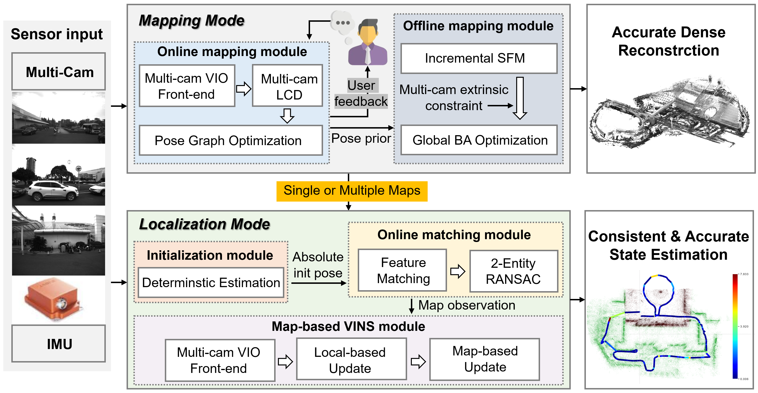
Figure 1: Overview of the proposed VILO system framework. In mapping mode, the system receives real-time multi-sensor data inputs into the online mapping module for initial map construction, and provides mapping quality feedback to the user, allowing for timely adjustments to the data collection strategy. Then the offline mapping module perform two-stage high-precision map construction and support dense reconstruction output. In localization mode, the system uses single or multiple isolated maps constructed in mapping mode for map-based consistent, accurate and real-time state estimation. Specific details can be found in Sec. III. LCD: Loop closure detection, SFM: structure-from-motion, BA: bundle adjustment.

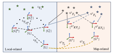
Figure 2: Illustration of each frame. There are two kinds of observations in the proposed system, the local observation (the blue shade part) and the map observation (the pink shade part).

II Notation

II-A Coordinate system

As shown in Table II and Fig. 2, there are five kinds of frames which can be categorized into the local-related frames including $\{L\}$, $\{I_{t}\}$ and {$C^{k}_{t}\}$, and map-related frames including $\{G_{i}\}$ and $\{{}^{G_{i}}KF_{j}\}$. For brevity, we consider only two isolated maps on Fig. 2. An arrow from the feature point to the frame indicates that the feature was observed at the corresponding time.

TABLE II: The definition of involved frames.

$\{L\}$	The local inertial frame, which is a fixed frame defined by the initial pose of VIO (cf. $\{L\}$ in Fig. 2).
$\{I_{t}\}$	The IMU (body) frame at timestamp $t$, which is attached to the robot. VIO online estimates the transformation between $\{L\}$ and $\{I_{t}\}$, i.e., ${}^{L}\mathbf{T}_{I_{t}}$.
$\{C^{k}_{t}\}$	The $k$-th ($k$ = 1,2,$\cdots$,$m$) camera (image) frame at timestamp $t$ .
$\{G^{i}\}$	The $i$-th map frame. All the $i$-th-map-related information (including map keyframes and map features) is based on this frame (cf. $\{G^{1}\}$ and $\{G^{2}\}$ in Fig. 2).
$\{{}^{G^{i}}KF_{j}\}$	The $j$-th image keyframe of the $i$-th pre-built map, whose pose ${}^{G^{i}}\mathbf{T}_{KF_{j}}$ is represented in {$G^{i}$} (cf. {${}^{G^{1}}KF_{1}$} and {${}^{G^{2}}KF_{1}$} in Fig. 2). After the $i$-th map is built, the keyframes $\{{}^{G^{i}}KF_{j}\}$ are fixed.

For the transformation between two frames, we use ${}^{A}\mathbf{T}_{B}$ to denote the transformation from $\{B\}$ to $\{A\}$ as

$${{}^{A}{\mathbf{T}}_{B}}\triangleq\begin{bmatrix}{}^{A}{\mathbf{R}}_{B}&{}^{A}{\mathbf{p}}_{B}\vskip 4.30554pt\\ \mathbf{0}_{1\times 3}&1\end{bmatrix}$$ (1)

where ${}^{A}\mathbf{R}_{B}$ is the rotation matrix and ${}^{A}\mathbf{p}_{B}$ represents the translation vector. Thus, the extrinsic transformation between $\{C^{i}\}$ and $\{C^{i+1}\}$ is ${}^{C^{i}}\mathbf{T}_{C^{i+1}}$.

II-B System state

For the system state definition, we denote the 6 Degree of Freedom (DoF) state, which contains the rotation and translation part as:

$$^{A}\mathbf{x}_{B}=[\begin{array}[]{cc}{}^{A}\mathbf{q}{{}^{\top}_{B}}&{}^{A}\mathbf{p}{{}^{\top}_{B}}\end{array}]^{\top}$$ (2)

where ${}^{A}\mathbf{q}{{}_{B}}$ denotes the JPL quaternion [17] and is corresponding to the rotation matrix ${}^{A}\mathbf{R}_{B}$ which represents the rotation from the $\{B\}$ to $\{A\}$. ${}^{A}\mathbf{p}_{B}$ represents the translation vector from the $\{B\}$ to $\{A\}$. Thus, the estimated IMU state is denoted as ${}^{G}\mathbf{x}_{I}$, the $1$st to $m$-th camera state is denoted as ${}^{G}\mathbf{x}_{C^{1}}$ to ${}^{G}\mathbf{x}_{C^{m}}$. The extrinsic between IMU and the $k$-th camera is defined as ${}^{I}\mathbf{x}_{C^{k}}$. Besides, the position of $i$-th triangulation feature points is denoted as ${}^{G}\mathbf{F}_{i}$.

III Multi-cam Multi-map Visual Inertial Localization System

III-A Problem statement

A complete VILO system should consists of a mapping mode as well as a map-based localization mode. Mapping mode is to obtain the precise pose of each keyframe (e.g. $\{^{G^{1}}KF_{1}\}$) and position of each triangulated points (e.g. ${}^{G^{1}}\mathbf{F}_{1}$) in each map frame (e.g. $\{G^{1}\}$).

As for localization mode, we first need to obtain the transformation from the map frame to the local frame (e.g. $\{^{G^{1}}\mathbf{T}_{L}\}$) through initialization module. Then we can combine the results of visual inertial odometry, ${}^{L}\mathbf{T}_{I_{t}}$ to get the localization results in map frame. Furthermore, by matching the observations of the current camera with the map keyframes (e.g. {$C^{1}$} and {${}^{G^{1}}KF_{1}$}), we can obtain additional map observations to mitigate the drift of the odometry.

III-B System Overview

The framework of the proposed VILO system is depicted in Fig. 1. In the system design, particular attention was paid to the practical requirements of users when employing the VILO system, leading to the tailored design of corresponding modules to meet these demands.

Mapping mode. From a user perspective, it has two stages: data collection and data processing. During the application, the user often lack professional mapping knowledge. Thus, in order to avoid poor data quality leading to the failure of mapping, it is necessary to have timely online feedback on the quality of the collected data during the collection phase. Therefore, we develop an online mapping module (see Sec. III-C1) to swiftly generate a rough initial map, thus promptly providing feedback on mapping quality to the user. Then after obtaining high-quality mapping data in this way, we perform offline mapping module (see Sec. III-C2) to provide accurately optimized 3D reconstruction for localization mode.

Localization mode. Users mainly need the ability to access real-time localization results on the pre-built multiple maps. In addition, practical applications necessitate computational efficiency due to the limited computing power of local computing platforms. In response to the aforementioned requirements, we develop an initialization module (see Sec. III-D1) and an online matching module (see Sec. III-D2) to acquire map-based observations and deliver them to the lightweight map-based VINS module (see Sec. III-D3), facilitating consistent, accurate, and real-time state estimation.

III-C Mapping

For mapping mode, we will primarily introduce how to construct an accurate visual map using observations from surround-view multi-cameras. However, if the robot is also equipped with external data sources such as LiDAR or GPS, we support building a more accurately scaled visual map based on these absolute position observations. We will now introduce these two approaches separately.

III-C1 Online visual mapping module

The overall process of the online mapping module is shown in Fig. 3. We use the multi-camera SLAM module to run in real-time and provide feedback to guide user’s data collection behavior.

Multi-camera SLAM. The multi-camera SLAM module can be primarily divided into three parts: multi-camera visusal inertial odometry (VIO) front-end, loop closure detection, and back-end optimization.

To achieve robust front-end estimation, we employ OpenVINS [16], a versatile platform offering a modular on-manifold EKF-based VIO that facilitates real-time estimation of IMU trajectories. Despite the swiftness of the filtering approach, its precision is compromised by accumulation linearization errors [18]. To address this issue, we have integrated a loop detection and pose graph optimization into our module. For loop detection, we deploy DBoW2 [19], a cutting-edge bag-of-words place recognition method, combined with 4 DoF pose graph optimization within VINS-Mono [20].

Nonetheless, the prevailing methods for state estimation [21] [22] predominantly rely on observations from a single camera for loop detection. Loop detection tends to fail due to the limited field of view observed by a monocular camera, which is typically mounted facing forward. In typical environments like urban or campus settings, the forward-facing camera often captures extensive road surface with limited structural information, while more structured details are present on buildings to the sides. Therefore, we add observations from left camera to assist, ensuring more robust loop detection. For further details the readers are referred to part 2 in [23].

Data quality feedback. During the process of data collection, excessive movement can lead to blurry images or large perspective differences between adjacent images, which can pose great challenge of image feature matching and affect the quality of the final mapping. The front-end of multi-camera SLAM also involves the process of image feature matching, so when the multi-camera SLAM algorithm fails, it indicates poor image capture quality. One of the manifestations of the failure of the multi-camera SLAM algorithm is the sudden increase in estimated velocity in the state variables. Additionally, even if the algorithm does not fail, moving at a high speed can also lead to the two image quality issues mentioned above. Thus, we utilize velocity as feedback to guide users to either restart or conclude data collection.

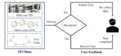
Figure 3: Online mapping process.

III-C2 Offline visual mapping module

Traditional visual mapping methods that utilize multiple cameras [24] often fix all cameras under a unified frame, creating a setup akin to a wide-angle camera, and integrate an IMU for enhanced system functionality. While these techniques significantly enhance pose estimation capabilities, they are prone to injecting additional noise into the reconstruction results, largely due to challenges associated with precise extrinsic calibration and temporal synchronization. Furthermore, errors in both extrinsic and intrinsic calibrations can lead to inaccurately scaled reconstructed scenes. To address these issues, this module incorporates extrinsic parameters as observations within the optimization process and proposes a two-stage Structure-from-Motion (SfM) approach [25].

STAGE I. We initiate our process by employing the traditional incremental SfM algorithm, COLMAP [26], to generate an initial map. To prevent suboptimal initial values from impairing the accuracy of subsequent optimization, we utilize the trajectory estimated by a multi-camera VINS as a prior to the incremental SfM algorithm. Given that COLMAP adjusts the overall scale during this procedure, we approximate the 3D similarity transformation between our initial estimates and the real-world towards the end of this phase. We establish the pose of the map camera at the beginning time as the global frame, and employ the extrinsic parameters of each camera to ascertain the poses of all cameras involved. Subsequently, we apply the geo-registration function within COLMAP to transform all camera poses and 3D points, ensuring alignment and accuracy in the reconstructed environment.

STAGE II. We perform the global BA optimization, considering both the multi-camera extrinsic constraint and the reprojection errors derived from the reconstruction results of the previous stage as:

$$E=E_{proj}+E_{extrinsic}$$ (3)

where $E_{proj}$ is the reprojection error of the 3D points of the initial map and $E_{extrinsic}$ is the relative pose error. For more technical details, please refer to [23].

Through the optimizations in the previous two steps, an accurate sparse map of the scene can be obtained, which is suitable for subsequent online applications. However, some other applications in the robotics domain, such as path planning, inspection, and object detection, require dense maps. Since our mapping results are compatible with the COLMAP format, we can directly leverage COLMAP’s interfaces to obtain a dense reconstruction of the scene.

III-C3 External data-source mapping module

During the mapping process, to acquire more information, collectors often carry additional sensors such as LiDAR and GPS devices. Unlike vision sensors that require algorithms to recover the scale of the real world, the data obtained by these sensors carries absolute scale information in itself. As a result, it can provide maps with more accurate scales and improve the accuracy of localization in large-scale localization tasks.

Our algorithm supports the integration of such sensor information to obtain a more precise map. Firstly, we convert the sensor data into 6 DoF pose observations (e.g., for LiDAR, this is done through LiDAR odometry). Utilizing the extrinsic parameters and timestamps between the sensors and the camera, we perform linear interpolation to obtain the pose of the camera at corresponding moments. This pose is then used in the STAGE I to triangulate the images and perform global bundle adjustment (BA) to obtain initial map estimates. These initial estimates are further optimized in the STAGE II as described above.

Finally, to align the optimized map with a given absolute frame, we utilize the initially obtained 6 DoF pose aligned with the images. Using a least squares approach, we estimate the transformation between the current map frame and the absolute pose observations, effectively transforming the map into the desired absolute frame.

III-D Localization

The goal of the localization mode is to achieve consistent, accurate and real-time state estimation w.r.t map frame. To achieve this, we design an initialization module at the beginning of the operation to obtain a relative pose from the map origin to the current odometry origin with deterministic optimality. Subsequently, keyframes are selected at a certain frequency, and their matching results with the map points are obtained through an online matching module. Based on these matching results, map-based VINS module reduces odometry drift, corrects the extrinsics between the map and current odometry, and thus achieves precise localization in the map.

III-D1 Initialization module

The initialization module needs to associate current visual-IMU observations with a pre-built map and calculate the current camera’s pose relative to the pre-built map’s frame. This aligns the odometry’s origin to the map’s absolute frame. Next, we will first discuss the characteristics that the initialization module needs to have, based on application requirements. Then, we will introduce the proposed efficient deterministic convergence estimation algorithm.

Robustness to extreme outliers. In practical applications, successful initialization is critical for accurate real-time pose estimation in map frame. Therefore, deterministic convergence of the initialization module’s estimation is of paramount importance. The computation time requirement can be relaxed accordingly, as users can tolerate a delay during the initialization phase to ensure its correctness. Therefore, RANSAC-based probabilistic optimal pose estimation methods[27, 28] are unsuitable, as significant appearance and viewpoint changes may occur during the robot’s long-term operation, leading to a limited number of feature matches and a potentially high outlier rate during initialization. Due to its sampling nature, RANSAC and similar methods struggle to ensure successful estimation under extreme outlier rates. Existing guaranteed optimal estimation methods[29, 30, 31], require exhaustive searches through feature and solution spaces, resulting in high computational complexity that is impractical for large-scale problems, such as when the number of feature matches exceeds 100.

To address this, we propose a minimal solution-based deterministic convergence algorithm capable of handling mismatch rates as high as 95% within seconds, specifically for the initialization module. This includes deriving an inertia-enhanced minimal solution for camera pose estimation and decoupling the rotation and translation solution spaces based on this minimal solution. Consequently, we propose an efficient deterministic convergence framework for outlier rejection.

Minimal solution. Due to the observability of the robot’s pitch and roll angles provided by inertial measurements[32], we can neutrally align the query camera frame with the map frame. This reduces the degrees of freedom in the pose estimation problem of the query relative to the map frame from 6DoF to 4DoF, specifically including 1DoF for the yaw rotation angle and 3DoF for translation. For the initialization module, the task is to estimate the transformation ${}^{G^{1}}\mathbf{T}_{L}$ from the initial VIO frame to the map frame. Given the known extrinsic calibration information between the IMU and the camera, the problem can be transferred to solving for the pose ${}^{G^{1}}\mathbf{T}_{C^{k}_{1}}$ of the $k$-th camera at first timestamp relative to the map frame. The unknowns in ${}^{G^{1}}\mathbf{T}_{C^{k}_{1}}$ can be represented as follows:

$$^{G^{1}}\mathbf{T}_{C^{k}_{1}}\triangleq\begin{bmatrix}\mathbf{R}(\alpha)&\mathbf{t}\vskip 4.30554pt\\ \mathbf{0}_{1\times 3}&1\end{bmatrix}$$ (4)

where $\alpha$ is the unknown yaw angle and $\mathbf{t}$ is the unknown translation from the query camera frame to the map frame. At this point, the problem becomes solving for the 4DoF pose based on the 2D-3D observations obtained from matching the current image with the map. To solve this problem, we introduce the geometric constraint of point collinearity based on the camera’s projection model. Specifically, for each 2D-3D inlier match $\mathbf{u}_{i}$ and $\mathbf{F}_{i}$, the 3D map points in the query camera frame should be collinear with the projection ray defined by the camera’s optical center and the 2D feature point. This collinearity constraint can be expressed as follows:

$$\frac{\mathbf{R}_{1}\mathbf{F}_{i}+t_{x}}{{v}_{i,x}}=\frac{\mathbf{R}_{2}\mathbf{F}_{i}+t_{y}}{{v}_{i,y}}=\mathbf{R}_{3}\mathbf{F}_{i}+t_{z}$$ (5)

where $\mathbf{R}(\theta)\triangleq(\mathbf{R}_{1}^{\top},\mathbf{R}_{2}^{\top},\mathbf{R}_{3}^{\top})^{\top}$ and $\mathbf{t}\triangleq(t_{x},t_{y},t_{z})^{\top}$. And

$$\mathbf{v}_{i}\triangleq\left(\begin{array}[]{c}{v}_{i,x}\\ {v}_{i,y}\\ 1\\ \end{array}\right)=\mathcal{K}^{-1}\left(\begin{array}[]{c}\mathbf{u}_{i}\\ 1\\ \end{array}\right)$$ (6)

where $\mathcal{K}$ is the intrinsic parameters.

Two independent constraints can be obtained from (5). Given another 2D-3D match, two additional constraints can be derived. By combining these four constraints, the translation component can be eliminated, resulting in a constraint that only involves the unknown yaw angle, denoted as

$$d(\alpha)=0$$ (7)

The detailed derivation of this constraint is referred to our previous work[33]. By solving this constraint, we can obtain the analytical solution for the yaw angle. Substituting this solution back into the original four constraints, we can derive the analytical expressions for the translation components. Thus, from any two sets of 2D-3D matches, the minimal solution for the unknown 4DoF pose can be determined.

Deterministic optimal search. To achieve robustness against extreme outlier rates, we propose an efficient deterministic convergence framework based on this minimal solution, ensuring optimality. Specifically, during the derivation of the above minimal solution, we found that solving for the unknown yaw angle of rotation can be decoupled from translation. Using (7), we can obtain a translation invariant measurement (TIM). Thus, we now construct a consensus maximization problem solely related to rotation to solve for the optimal yaw angle as follows:

$$\max_{\alpha,\{z_{ij}\}}\sum z_{ij}$$ (8)

$$s.t.~~~~z_{ij}\|d_{ij}(\alpha)\|\leq n_{ij}$$ (9)

where $i$ and $j$ are the indices of any two sets of 2D-3D correspondences. $n_{ij}$ is the TIM noise, $z_{ij}=1$ means that the two correspondences are inliers, otherwise, $z_{ij}=0$. $\|\cdot\|$ denotes the Euclidean norm.

Then an adaptive voting algorithm is designed to search for the 1 DoF rotation, obtaining the globally optimal yaw angle $\hat{\alpha}$ and eliminating a large number of erroneous matches. Additionally, we introduce a discretized search to further accelerate the process. After obtaining the optimal yaw angle, we can fix the rotation component and formulate a consensus maximization problem that only pertains to translation:

$$\max_{\mathbf{t},\{z_{i}\}}\sum z_{i}$$ (10)

$$s.t.~~~~z_{i}\|\mathbf{u}_{i}-\pi(\mathbf{R}(\hat{\alpha})\mathbf{F}_{i}+\mathbf{t},\mathcal{K})\|\leq\mathbf{n}_{i}$$ (11)

where $\pi$ is the camera projection function and $\mathbf{n}_{i}$ is the bounded measurement noise. And $i$ is the correspondence index in the obtained maximal consensus set in rotation estimation. Then we formulate a maximum clique finding problem to search the globally optimal 3 DoF translation efficiently. Finally, a prioritized optimal search framework is used to ensure the global optimality of solving the two sub-problems. For more technical details, please refer to [33].

III-D2 Online matching module

The above-mentioned initialization module can achieve globally optimal pose matching results in seconds, enabling high-precision localization results during the initialization phase. However, after completing the initialization steps, in order to obtain more observations within a certain time duration to reduce the odometry drift, a trade-off between efficiency and accuracy needs to be made. Therefore, we adopt a more efficient RANSAC-based strategy of instant local optimization to strike a balance between efficiency and accuracy.

Real time sampling-based framework. Specifically, we reduce the minimal required number of point matches for pose estimation from 3 to 2 by aligning the direction of gravity with the aid of inertial measurements, detailed in Sec. III-D1. Embedding the derived 2P-based minimal solution into RANSAC framework, we propose a sampling-based 2P RANSAC framework for robust feature matching. Given the relationship expressed by $P$, the success rate of the RANSAC algorithm within $k$ iterations, and $w$, the inlier rate, we derive the following equation:

$$1-P=(1-w^{n})^{k}$$ (12)

This relationship elucidates that, with a constant number of iterations, enhancing the inlier rate $w$ or reducing the minimal number of elements $n$ required to compute the model results in an increased probability of success for RANSAC. We have decreased the minimal number $n$ from 3 to 2 by incorporating inertial measurements which enable a more robust estimation with fewer samples. Additionally, we have implemented a feature scoring methodology aimed at augmenting the inlier rate $w$ within a RANSAC sample. Therefore, compared to traditional methods that require 3 or 4 pairs of feature matches for pose estimation, the proposed minimal solutions enhance the robustness of the RANSAC-based algorithm to outlier rates from 60% to 80%.

Furthermore, we have developed a multi-camera minimal solution, termed MC2P, which consolidates observations from multiple views, effectively increasing the count of inliers and thereby enhancing the robustness and accuracy of the model estimation process. With this robust and efficient estimation algorithm, our online matching module achieves robust outlier rejection for multi-camera feature matching, thereby providing accurate map observations for the subsequent Map-based VINS module. For more details the reader is referred to our previous work [34].

III-D3 Map-based VINS module

Given good initialization of localization and imgae matching observations, how to utilize this information to obtain real-time accurate localization in the pre-built map is a problem that needs to be addressed. Specifically, we propose a map-based VINS module which utilizes a filter-based framework that consistently and efficiently fuses multiple isolated maps into the system to improve the localization accuracy.

System state. We extend the state of Open-VINS to get the augmented system state $\mathbf{x}_{t}$:

$$\mathbf{x}_{t} =\begin{bmatrix}\mathbf{x}_{VIO_{t}}^{\top}&\mathbf{x}_{SW_{t}}^{\top}&\mathbf{x}_{\tau_{t}}^{\top}&\mathbf{x}_{KF_{t}}^{\top}\end{bmatrix}^{\top}$$ (13)

$$\mathbf{x}_{VIO_{t}} =\begin{bmatrix}{}^{I_{t}}\mathbf{q}_{L}^{\top}&{}^{L}\mathbf{v}_{I_{t}}^{\top}&{}^{L}\mathbf{p}_{I_{t}}^{\top}&\mathbf{b}_{g_{t}}^{\top}&\mathbf{b}_{a_{t}}^{\top}\end{bmatrix}^{\top}$$

$$\mathbf{x}_{SW_{t}} =\begin{bmatrix}{}^{I_{t-1}}\mathbf{q}_{L}^{\top}&{}^{L}\mathbf{p}_{I_{t-1}}^{\top}&\cdots&{}^{I_{t-B}}\mathbf{q}_{L}^{\top}&{}^{L}\mathbf{p}_{I_{t-B}}^{\top}\end{bmatrix}^{\top}$$

$$\mathbf{x}_{\tau_{t}} =\begin{bmatrix}{}^{G^{1}_{t}}\mathbf{q}_{L}^{\top}&{}^{G^{1}_{t}}\mathbf{p}_{L}^{\top}&\cdots&{}^{G^{N}_{t}}\mathbf{q}_{L}^{\top}&{}^{G^{N}_{t}}\mathbf{p}_{L}^{\top}\end{bmatrix}^{\top}$$

$$\mathbf{x}_{KF_{t}} =\begin{bmatrix}\cdots{}^{G^{1}_{t}}\mathbf{q}_{kf_{j}}^{\top}\!&\!{}^{G^{1}_{t}}\mathbf{p}_{kf_{j}}^{\top}\cdots{}^{G^{N}_{t}}\mathbf{q}_{kf_{k}}^{\top}\!&\!{}^{G^{N}_{t}}\mathbf{p}_{kf_{k}}^{\top}\cdots\end{bmatrix}\!^{\top}$$

where $\mathbf{x}_{VIO_{t}}$ and $\mathbf{x}_{SW_{t}}$ form the original state of Open-VINS, $\mathbf{x}_{\tau_{t}}$ and $\mathbf{x}_{KF_{t}}$ are the augmented parts. To be specific, for $\mathbf{x}_{VIO_{t}}$, ${}^{I_{t}}\mathbf{q}_{L}$ is the unit quaternion that transforms a 3D vector from $\{L\}$ to $\{I_{t}\}$, ${}^{L}\mathbf{p}_{I_{t}}$ is the position of $\{I_{t}\}$ in $\{L\}$, ${}^{L}\mathbf{v}_{I_{t}}$ is the velocity of $\{I_{t}\}$ in the frame$\{L\}$, and $\mathbf{b}_{g_{t}}$ and $\mathbf{b}_{a_{t}}$ are the bias of gyroscope and accelerometer. VIO outputs the pose ${}^{L}\mathbf{T}_{I_{t}}\triangleq\{{}^{I_{t}}\mathbf{q}_{L},{}^{L}\mathbf{p}_{I_{t}}\}$. $\mathbf{x}_{SW_{t}}$ contains $B$ cloned historical body poses, which is the so-called sliding window. Suppose we have $N$ isolated pre-built maps, then the elements ${}^{G^{i}_{t}}\mathbf{q}_{L},\,{}^{G^{i}_{t}}\mathbf{p}_{L},\,i=1\cdots N$ represent the relative transformation between the local VIO frame $\{L\}$ and the $i$-th map frame $\{G^{i}\}$, i.e., the so-called augmented variable. $\mathbf{x}_{KF_{t}}$ contains a set of keyframe poses from $N$ isolated maps. For instance, ${}^{G^{1}_{t}}\mathbf{q}_{kf_{j}}$ and ${}^{G^{1}_{t}}\mathbf{p}_{kf_{j}}$ represent the orientation and the position of the $j$-th keyframe from the $1$st map, respectively.

State propagation. For the augmented system, with the state defined in (13), we have the following kinematics equations:

$$\left\{\begin{aligned} {}^{I_{t}}\dot{\mathbf{q}}_{L}&=\frac{1}{2}\Omega(\bm{\omega}_{m_{t}}-\mathbf{b}_{g_{t}}-\mathbf{n}_{g_{t}}){}^{I_{t}}\mathbf{q}_{L}&\\ {}^{L}\dot{\mathbf{v}}_{I_{t}}&=C(^{I_{t}}{\mathbf{q}}_{L})^{\top}(\mathbf{a}_{m_{t}}-\mathbf{b}_{a_{t}}-\mathbf{n}_{a_{t}})+\mathbf{g}\\ {}^{L}\dot{\mathbf{p}}_{I_{t}}&={}^{L}\mathbf{v}_{I_{t}}\\ \dot{\mathbf{b}}_{g_{t}}&=\mathbf{n}_{wg_{t}}\;\;\;\,\dot{\mathbf{b}}_{a_{t}}=\mathbf{n}_{wa_{t}}\\ {}^{G_{t}^{i}}\dot{\mathbf{q}}_{L}&=\mathbf{0}\;\;\;\;\;\;^{G_{t}^{i}}\dot{\mathbf{p}}_{L}=\mathbf{0}\\ {}^{G_{t}^{i}}\dot{\mathbf{q}}_{kf_{j}}&=\mathbf{0}\;\;\;\;^{G_{t}^{i}}\dot{\mathbf{p}}_{kf_{j}}=\mathbf{0}\\ \end{aligned}\right.$$ (14)

where we argue that the augmented variable and the keyframe pose from maps should be static. $C(\cdot)$ transforms a quaternion to a rotation matrix $\mathbf{R}$, $\bm{\omega}_{m_{t}}$ and $\mathbf{a}_{m_{t}}$ are the measurements from IMU in frame $\{L\}$, $\mathbf{n}_{g_{t}}$ and $\mathbf{n}_{a_{t}}$ are the measurement noises, $\mathbf{n}_{wg_{t}}$ and $\mathbf{n}_{wa_{t}}$ are the random walk noises, $\mathbf{g}=\begin{bmatrix}0&0&-9.81\end{bmatrix}^{\top}m/s^{2}$ is the gravitational acceleration in $\{L\}$. For a vector $\bm{\omega}\in\mathbb{R}^{3}$, we have

$$\Omega(\bm{\omega})=\begin{bmatrix}-\bm{\omega}_{\times}&\bm{\omega}\\ \bm{\omega}^{\top}&0\end{bmatrix}.$$

By discretizing (14), we can propagate the state from time step $t$ to time step $t+1$:

$$\mathbf{x}_{t+1|t}=\mathbf{f}(\mathbf{x}_{t},\mathbf{a}_{m_{t}}-\mathbf{n}_{a_{t}},\bm{\omega}_{m_{t}}-\mathbf{n}_{\omega_{t}})$$ (15)

where $\mathbf{f}(\cdot)$ is the discretized propagation function derived from (14), the subscript $t+1|t$ means the state is propagated from $t$ to $t+1$, with all the measurements up to time step $t$ being processed. Then, the state covariance can be propagated by

$$\mathbf{P}_{t+1|t}=\mathbf{\Phi}_{t+1|t}\mathbf{P}_{t}\mathbf{\Phi}_{t+1|t}^{\top}+\mathbf{G}_{t+1|t}\mathbf{Q}_{t}\mathbf{G}_{t+1|t}^{\top}$$ (16)

where $\mathbf{P}_{t}$ and $\mathbf{Q}_{t}$ are the system state covariance and the noise covariance, respectively. $\mathbf{\Phi}_{t+1|t}$ and $\mathbf{G}_{t+1|t}$ are the Jacobians of (15) with respect to the system state and the noise, respectively. $\mathbf{\Phi}_{t+1|t}$ is also called state transition matrix. For the detailed derivation, please refer to [35, 16].

As indicated in Fig. 2, there are two kinds of observation functions, the local feature based (the blue shade part) and the map feature based (the pink shade part).

Local observation function. For a local feature ${}^{L}\mathbf{F}_{i}$, online detected by the camera, we have the following local observation function:

$${}^{loc}\mathbf{y}_{t}^{i}=\mathrm{h}({}^{I_{t}}\mathbf{R}_{L}({}^{L}\mathbf{F}_{i_{t}}-{}^{L}\mathbf{p}_{I_{t}}))+{}^{loc}\bm{\gamma}_{t}^{i}$$ (17)

where for simplicity, we assume the extrinsic between the IMU and the camera is an identity matrix. ${}^{I_{t}}\mathbf{R}_{L}$ is the rotation matrix from $\{L\}$ to $\{I\}$. $\mathrm{h}(\cdot)$ is the camera projection function that projects a 3D feature in the camera frame into the 2D image plane. ${}^{loc}\bm{\gamma}_{t}^{i}$ is the noise of the local observation.

With (17), the error of the local observation can be computed by:

$${}^{loc}\mathbf{r}_{t}^{i} \triangleq\mathrm{h}({}^{I_{t}}\mathbf{R}_{L}({}^{L}\mathbf{F}_{i_{t}}-{}^{L}\mathbf{p}_{I_{t}}))+{}^{loc}\bm{\gamma}_{t}^{i}-$$ (18)

$$\;\;\;\;\;\mathrm{h}({}^{I_{t}}\hat{\mathbf{R}}_{L}({}^{L}\hat{\mathbf{F}}_{i_{t}}-{}^{L}\hat{\mathbf{p}}_{I_{t}}))$$

$${}^{loc}\mathbf{r}_{t}^{i} ={}^{loc}\mathbf{H}_{\mathbf{x}_{t}}^{i}\tilde{\mathbf{x}}_{t}+{}^{loc}\mathbf{H}_{{}^{L}\mathbf{F}_{i_{t}}}{}^{L}\tilde{\mathbf{F}}_{i_{t}}+{}^{loc}\bm{\gamma}_{t}^{i}$$

where $\hat{\cdot}$ represents the estimated value of the variable, $\tilde{\cdot}$ represents the error between the true value and the estimated value of the variable. ${}^{loc}\mathbf{H}_{x_{t}}^{i}$ and ${}^{loc}\mathbf{H}_{{}^{L}\mathbf{F}_{i_{t}}}$ represent the Jacobian matrices of $\mathrm{h}$ with respect to $\mathbf{x}_{t}$ and ${}^{L}\mathbf{F}_{i_{t}}$, respectively.

Within the MSCKF framework [35], local features are not retained in the state vector, necessitating the application of null-space projection to the Jacobian matrix of the observation function $\mathrm{h}$ concerning each local feature ${}^{L}\mathbf{F}_{i_{t}}$. This ensures that irrelevant components are eliminated effectively. The presence of a sliding window $\mathbf{x}_{SW}$ in our methodology provides a significant advantage. It allows a local feature to be observed by not only the current camera frame but also by multiple preceding frames. Consequently, each local feature is associated with multiple (at least two, $n\geq 2$) local observation functions. By aggregating these observation functions, the Jacobian matrix’s row count (representing the observations, $2n$) exceeds its column count (representing the local feature’s dimensionality, 3). This dimensional relationship ensures the existence of a left null-space in the Jacobian matrix of $\mathrm{h}$ concerning ${}^{L}\mathbf{F}_{i_{t}}$, which is crucial for effectively eliminating undesired dependencies. For a more in-depth explanation, readers are encouraged to consult [35].

Map-based observation function. For a feature from a pre-built map, it can be observed by the current camera $C_{t}$ and keyframes ${}^{G^{i}}KF_{j}$ from different maps, as indicated by the pink shade part of Fig. 2. Suppose there is a feature ${}^{G^{k}}\mathbf{F}_{i}$ from the $k$-th map, observed by the $j$th keyframe ${}^{G^{k}}KF_{j}$ in the $k$-th map. Besides, ${}^{G^{k}}\mathbf{F}_{i}$ can also be observed by the current camera frame $\{C\}$ and the $l$-th keyframe ${}^{G^{s}}KF_{l}$ in the $s$-th ($s\neq k$) map. For example, by setting $k=1,i=1,j=1,s=2,l=1$, the situation is exactly described by Fig. 2. Then, there exist three observation functions:

$$^{cam}\mathbf{y}_{t}^{ki}\!=\!\mathrm{h}\!\left[{}^{I_{t}}\mathbf{R}_{L}({}^{G_{t}^{k}}\mathbf{R}_{L}^{\top}({}^{G^{k}}\mathbf{F}_{i_{t}}\!\!-\!\!{}^{G_{t}^{k}}\mathbf{p}_{L})-{}^{L}\mathbf{p}_{I_{t}})\right]+{}^{cam}\bm{\gamma}_{t}^{ki}$$ (19)

$$^{{}^{G^{k}}KF_{j}}\mathbf{y}_{t}^{ki}=\mathrm{h}\left[{}^{G_{t}^{k}}\mathbf{R}_{KF_{j}}^{\top}({}^{G^{k}}\mathbf{F}_{i_{t}}-{}^{G^{k}_{t}}\mathbf{p}_{KF_{j}})\right]+{}^{{}^{G^{k}}KF_{j}}\bm{\gamma}_{t}^{ki}$$ (20)

$${}^{{}^{G^{s}}KF_{l}}\mathbf{y}_{t}^{ki} =\mathrm{h}\left[{}^{G_{t}^{s}}\mathbf{R}_{KF_{l}}^{\top}\left[{}^{G_{t}^{s}}\mathbf{R}_{L}{}^{G_{t}^{k}}\mathbf{R}_{L}^{\top}({}^{G^{k}}\mathbf{F}_{i_{t}}-{}^{G^{k}_{t}}\mathbf{p}_{L})\right.\right.$$ (21)

$$\;\;\;\;\left.\left.+{}^{G_{t}^{s}}\mathbf{p}_{L}-{}^{G_{t}^{s}}\mathbf{p}_{KF_{l}}\right]\right]+{}^{{}^{G^{s}}KF_{l}}\bm{\gamma}_{t}^{ki}$$

where ${}^{cam}\mathbf{y}_{t}^{ki}$, ${}^{{}^{G^{k}}KF_{j}}\mathbf{y}_{t}^{ki}$ and ${}^{{}^{G^{s}}KF_{l}}\mathbf{y}_{t}^{ki}$ represent the observations to the feature ${}^{G^{k}}\mathbf{F}_{i}$ by the current camera, the map keyframe ${}^{G^{k}}KF_{j}$ and the map keyframe ${}^{G^{s}}KF_{l}$, respectively. ${}^{cam}\bm{\gamma}_{t}^{ki}$, ${}^{{}^{G^{k}}KF_{j}}\bm{\gamma}_{t}^{ki}$ and ${}^{{}^{G^{s}}KF_{l}}\bm{\gamma}_{t}^{ki}$ are the corresponding observation noises. For simplicity, we assume the extrinsic ${}^{I}\mathbf{T}_{C}$ between the IMU and the camera is an identity matrix.

Similar to (18), we have the following map-based observation errors derived from (19)-(21):

$${}^{cam}\mathbf{r}_{t}^{ki}={}^{cam}\mathbf{H}_{\mathbf{x}_{t}}^{ki}\tilde{\mathbf{x}}_{t}+{}^{cam}\mathbf{H}_{{}^{G^{k}}\mathbf{F}_{i_{t}}}{}^{G^{k}}\tilde{\mathbf{F}}_{i_{t}}+{}^{cam}\bm{\gamma}_{t}^{ki}$$ (22)

$${}^{{}^{G^{k}}KF_{j}}\mathbf{r}_{t}^{ki}={}^{{}^{G^{k}}KF_{j}}\mathbf{H}_{\mathbf{x}_{t}}^{ki}\tilde{\mathbf{x}}_{t}+{}^{{}^{G^{k}}KF_{j}}\mathbf{H}_{{}^{G_{k}}\mathbf{F}_{i_{t}}}{}^{G^{k}}\tilde{\mathbf{F}}_{i_{t}}+{}^{{}^{G^{k}}KF_{j}}\bm{\gamma}_{t}^{ki}$$ (23)

$${}^{{}^{G^{s}}KF_{l}}\mathbf{r}_{t}^{ki}={}^{{}^{G^{s}}KF_{l}}\mathbf{H}_{\mathbf{x}_{t}}^{ki}\tilde{\mathbf{x}}_{t}+{}^{{}^{G^{s}}KF_{l}}\mathbf{H}_{{}^{G^{k}}\mathbf{F}_{i_{t}}}{}^{G^{k}}\tilde{\mathbf{F}}_{i_{t}}+{}^{{}^{G^{s}}KF_{l}}\bm{\gamma}_{t}^{ki}$$ (24)

In the context of our MSCKF implementation, we do not retain the map feature ${}^{G^{k}}\mathbf{F}_{i_{t}}$ in the state vector. Therefore, the Jacobian matrices associated with ${}^{G^{k}}\mathbf{F}_{i_{t}}$ require null-space projection. As detailed in equations (19) through (21), each map feature ${}^{G^{k}}\mathbf{F}_{i_{t}}$ is linked to at least two observation functions. This configuration arises unless the feature is observed solely by the keyframe in the $k$-th map, in which case (21) vanishes. The presence of multiple observation functions for each map feature allows us to identify and apply a left null-space matrix, effectively removing the components related to ${}^{G^{k}}\tilde{\mathbf{F}}_{i_{t}}$ from the state update equations.

It is important to highlight that the purpose behind introducing (23) and (24) is to eliminate the parts of the estimation related to map features, particularly considering the uncertainty in map data. In our methodology, the poses of map keyframes and the positions of map features are treated as fixed variables. This approach is adopted because the maps previously constructed are typically accurate, and updating this map data during real-time operations can be computationally intensive and may not significantly enhance performance. For more comprehensive details and the theoretical underpinnings of this approach, readers are referred to our previous publications [36] [37].

TABLE III: Comparison of popular datasets.

Dataset	Multi-camera	Additional sensors	Multi-session	Changes	Out/indoors	Camera motion
EuROC[38]	stereo	LiDAR,IMU	check mark button	cross mark	cross markcheck mark button	UAV
KITTI[39]	stereo	LiDAR,IMU	cross mark	man running	check mark buttoncross mark	Car
KITTI360[40]	stereo+2	LiDAR,IMU	cross mark	man running	check mark buttoncross mark	Car
Newer College[41]	stereo+2	LiDAR,IMU	check mark button	last quarter moon	check mark buttoncheck mark button	Hand-held
M2DGR[42]	stereo+5	LiDAR,IMU,Infrared,GNSS,Event	check mark button	last quarter moon	check mark buttoncheck mark button	Ground Robot
NCLT[43]	6	LiDAR,IMU	check mark button	man running cloud with rain last quarter moon fallen leaf building construction	check mark buttoncheck mark button	Ground Robot
Ours	2stereo+3	LiDAR,GPS/INS,IMU	check mark button	man running cloud with rain last quarter moon fallen leaf building construction triangular ruler	check mark buttoncheck mark button	Car

• “Multi-session” means collecting data at the same location at different times.

• The proposed dataset exhibits appearance and structural changes due to moving people/cars/furnitures man running, weather cloud with rain, lighting last quarter moon, but also long-term changes due to season fallen leaf changes, construction work building construction, as well as large viewpoint changes triangular ruler.

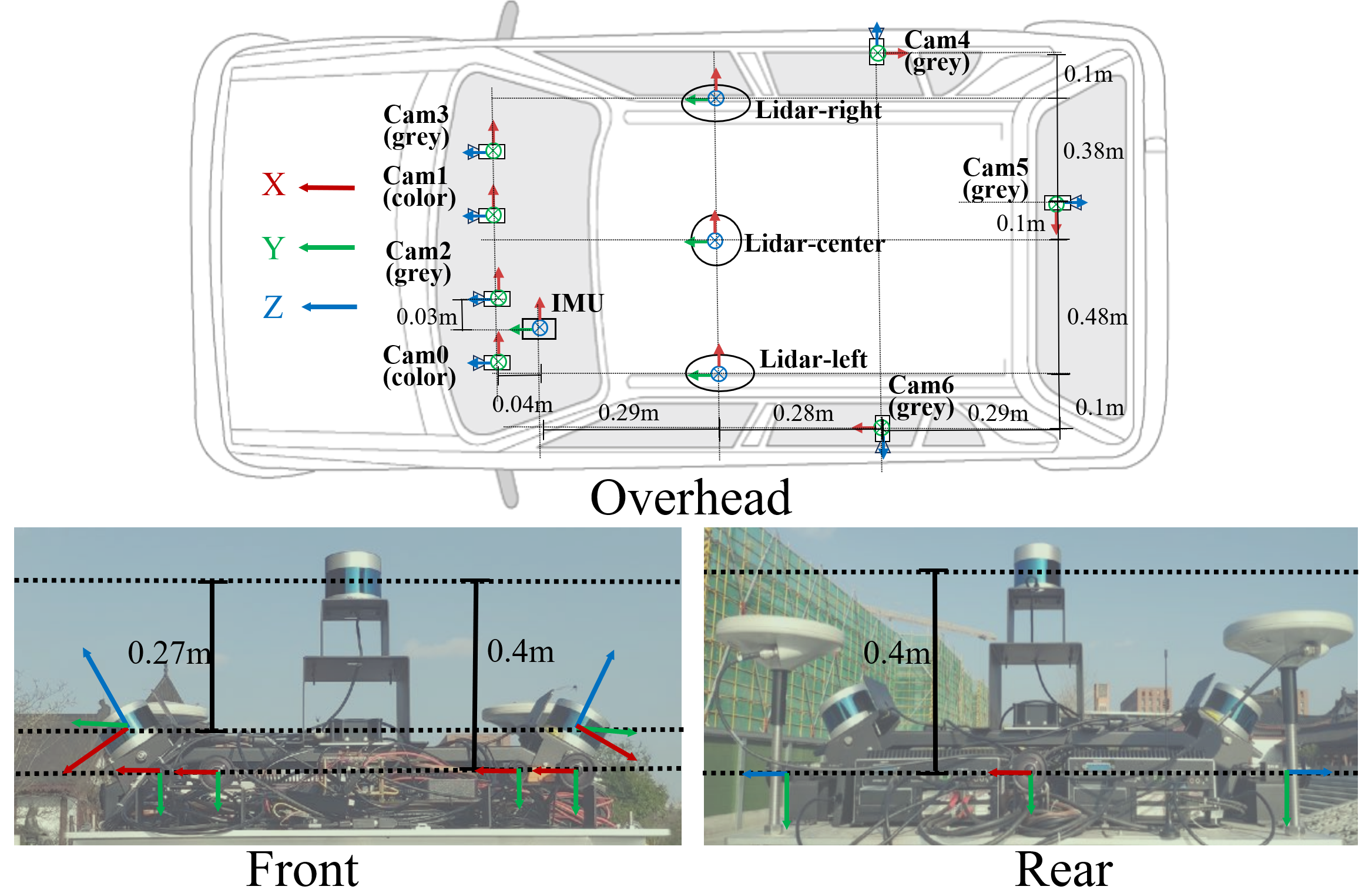
Figure 4: Multi-sensor data collection vehicle.

IV Multi-camera Long-term Dataset

To validate the effectiveness of the proposed VILO system, we require a dataset with surround multi-camera images, IMU, and external sensor data such as LiDAR and GPS, and it should include challenging long-term changes. However, current publicly available datasets are inadequate to meet these requirements as shown in Table III. Note that while the NCLT dataset has rich sensor data, its six cameras do not have overlapping views, thus lacking stereo images, which prevents the validation of stereo odometry algorithms. Consequently, we assemble a hardware setup to collect a multi-camera campus dataset in long-term operation. Specifically, a multi-sensor synchronization and data acquisition system is designed, and a dataset containing long-term variations is collected using this system. The core of this system is a synchronization module that can achieve hardware synchronization of sensors such as laser, camera, IMU, and INS, and has good scalability. Based on this, a multi-sensor data acquisition platform is built on a car. In a campus environment, road data under different conditions is collected by driving the vehicle.

TABLE IV: Configurations of data collection vehicles.

Sensor	Type	Hz	Specification
Front Color Camera	BFS-PGE-31S4C-C	16	$2048\times 1536$ 1
Front Grey Camera	BFLY-PGE-03S3M-CS	16	$648\times 488$ 1
Left&Right Fisheye	BFLY-PGE-03S3M-CS	16	$648\times 488$ 1
3D LiDAR(Top)	VLP-32C	10	$32$ 2
3D LiDAR(Side)	VLP-16	10	$16$ 2
IMU	Xsens MTi-700	400	-
INS	Applanix LVX	100	-

• ¹ resolution, ² number of channels.

IV-A Hardware platform configuration

As shown in Fig. 4, We design a multi-sensor hardware platform and install it on a vehicle for data collection. The detailed parameters of the sensors are provided in Table IV. Specifically, $4$ cameras are installed on the front of the platform, including $2$ color cameras forming a color stereo pair, and $2$ grey cameras forming a grey stereo pair, each with a baseline of approximately $50$cm. The color stereo cameras have higher resolution but lower frame rates, making them suitable for research in vehicle detection and pedestrian detection, among other perception-related studies. The grey stereo cameras have lower resolution and higher frame rates, and can be used for SLAM, visual localization and other research. Additionally, the platform is equipped with a fisheye camera on each of the left, right and rear sides, providing a wide field of view to ensure complete coverage around the vehicle. When combined with the grey stereo cameras, they can be used for research in visual localization. The top of the platform is equipped with a 32-channel laser, covering the surrounding environment and supporting research in laser-based positioning. Furthermore, a 16-channel laser scanner is installed on each side, covering the left and right sides of the vehicle, and suitable for research in environment perception.

IV-B Hardware synchronization design

The task of the synchronization module is to maintain a unified clock source and stamp the data from different sensors according to this clock source. The synchronization module must support commonly positioning perception sensors, such as camera, LiDAR, IMU, GPS, and INS. Furthermore, in order to ensure the quality of synchronization, it should be implemented through hardware rather than software as much as possible. Accordingly, we have designed a synchronization module with a MCU as the core, as shown in Fig. 5. The clock source of this module comes from the high-frequency IMU, and the pulse signal of the IMU is divided into different low-frequency sensors. In order to cope with both outdoor and indoor scenarios, two sets of implementations have been designed, with the outdoor solution utilizing GPS signals and supporting synchronized INS devices, while the indoor solution does not require GPS signals. The selection of sensors in the module is listed in Table V.

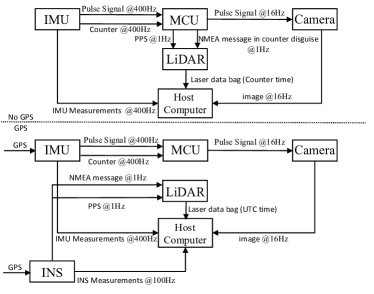
Figure 5: Two solutions for indoor (top) and outdoor (bottom) multi-sensor synchronization modules.

IV-B1 Outdoor implementation

The selected IMU can interface with GPS to update its internal Coordinated Universal Time (UTC) clock. Its output includes pulse signals and IMU messages, as shown in Fig. 5. The IMU outputs a rising edge pulse signal at the beginning of each sampling, which can be used to trigger other sensors. After the sampling is complete, the IMU outputs a message containing IMU measurements, a gradually increasing counter $k$, and the UTC time $u^{I}_{k}$. The counter $k$ represents the current serial number of IMU measurements, starting from 0 when the power is turned on, and incremented by $1$ after each output, i.e. $k=0,1,2,\cdots$. When IMU is connected to GPS, the UTC time is synchronized with the real world UTC time; without GPS, the UTC time starts from a fixed time when the power is turned on. In the outdoor solution, the host computer regards $u^{I}_{k}$ as the timestamp $t^{I}_{k}$ of the IMU upon receiving IMU information, i.e. $t^{I}_{k}=u^{I}_{k}$. It records the counter and IMU timestamp ($k$, $t^{I}_{k}$) and stores them in the buffer.

Synchronization between IMU and other sensors. The MCU simultaneously receives the pulse signals and IMU messages from the IMU. When the counter meets certain conditions, the MCU will output a pulse signal, which can be used to trigger other sensors. The synchronization between the IMU and the camera is achieved through the pulse signal of the IMU. The camera in this system is capable of external triggering. Whenever it receives a rising edge signal, the camera starts exposure, and after the exposure ends, it sends the image to the host computer. In order to achieve a camera running at 16Hz, with the known IMU output frequency of 400Hz, the condition for the counter is set to trigger when $k$ is divisible by 25. After receiving the image, the host computer will filter the IMU counter in the buffer and find the latest $k$ that satisfies being divisible by $25$. The corresponding timestamp $t^{I}_{k}$ is the timestamp of the current image.

In outdoor scenarios, INS is often included as a reference for localization and mapping. INS integrates GPS signals and internal IMU for pose fusion and estimation, ultimately providing relatively accurate pose information. Since both IMU and INS are connected to GPS, their UTC time is consistent with real-world UTC time, so INS only needs to use UTC time as its timestamp to achieve hardware synchronization with IMU. The synchronization between IMU and laser also relies on GPS. The laser system in this setup supports GPS synchronization, allowing it to receive National Marine Electronics Association (NMEA) messages from the NMEA to correct its internal clock and provide corresponding UTC time in the output laser data bags. NMEA messages for the outdoor solution come from INS, and IMU ultimately achieves hardware synchronization with the laser through INS as an intermediary. The entire process is shown in Fig. 5. Thus, the timestamps of the camera, laser, and INS are synchronized with the IMU, and all sensors are unified under a single time source.

TABLE V: Sensors synchronization requirements.

Sensor	Requirements
Camera	Capable of being triggered by external signals.
LiDAR	Capable of receiving GPS information to update
	the clock (NMEA protocol).
IMU	Capable of emitting pulse signals and  receiving
	GPS information to update the clock.
GPS	No specific requirements.
INS	Capable of outputting pulse signals and
	corresponding NMEA signals.

IV-B2 Indoor implementation

Compared with the outdoor implementation, the indoor implementation faces two issues: first, there is no GPS signal; second, there is no INS, therefore there is no NMEA message required for laser. The first issue will cause the UTC time of the IMU to be inconsistent with the real world UTC time. The adjustment made by the indoor solution is to record the first UTC time $u^{I}_{0}$ after receiving the IMU message and use the host computer time $t^{I}_{0}$ at that time as the timestamp for the IMU. For future messages, the IMU timestamp is set as $t^{I}_{k}=t^{I}_{0}+(u^{I}_{k}-u^{I}_{0})$.

Synchronization between IMU and other sensors. The synchronization between the IMU and the camera does not involve UTC time, so no changes are needed. As for the second issue, we propose a method to simulate NMEA messages through MCU and record the IMU’s counter in these messages. Specifically, the MCU sends an NMEA data bag to the laser at a fixed frequency (1 Hz). The UTC time $u^{p}$ of this bag is as follows:

$$u^{p}=u^{p}_{0}+\frac{k}{400}$$ (25)

where $u^{P}_{0}$ is a constant representing a fixed UTC time. When the upper computer receives the laser data, it decodes the UTC time $u^{l}$ of the laser. The counter corresponding to the laser is as follows:

$$k^{l}=400\Delta{u^{l}}$$ (26)

where $\Delta{u^{l}}=u^{l}-u^{p}_{0}$. It is worth noting that $k$ comes from IMU, which is an integer, whereas $k^{l}$ is a floating-point number. This is because the laser sampling process is independent of the IMU and its sampling time may be different from that of the IMU (strictly speaking, it is impossible for them to be the same). The timestamp of the laser is obtained by linear interpolation of adjacent IMU information: find two adjacent frames of IMU information, with their counters/timestamps being $k/t_{k}$ and $(k+1)/t_{k+1}$, satisfying $k<k^{l}<k+1$. The timestamp $t_{l}$ of the laser is as follows:

$$t_{l}=t_{k}+\dfrac{k^{l}-k}{k+1-k}(t_{k+1}-t_{k})=t_{k}+(k^{l}-k)(t_{k+1}-t_{k})$$ (27)

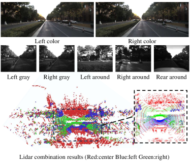
Figure 6: Examples of different sensor data from a data collection vehicle.

IV-C Data collection

For about nine months, data collection was carried out on Zhejiang University’s Zijingang Campus using the vehicle. An example of the collected data is illustrated in Fig. 6. As shown, the front color stereo cameras have a wide field of view, which is conducive to environment perception in front of the vehicle such as pedestrian and vehicle detection. The cameras effectively cover the entire surroundings of the collection vehicle, enhancing the robustness of SLAM to dynamic obstacles and improving the comprehensiveness of perception. The three lasers cover the entire periphery of the vehicle, with the top-mounted laser acquiring structural information from all directions, and the left and right lasers compensating for the blind spots on the sides of the vehicle. Additionally, the lateral lasers address the issue of sparse data near the vehicle caused by the top-mounted laser, thereby enhancing obstacle detection capabilities.

In order to assess the algorithm’s robustness during prolonged robot operation, the data collection vehicle repetitively traversed certain identical routes at different times, providing valuable material for long-term research in localization and perception. Some examples are presented in Fig. 7, where each row depicts the same location from nearly identical perspectives, yet exhibiting distinct visual appearances. The scenario is characterized by numerous unstructured objects, making it challenging to employ algorithms based on structured scenes, and representing a typical non-generic scenario. Short-term variations encompass moving vehicles, pedestrians, bicycles, and other interactive elements constantly engaging with the robot, as well as fluctuating lighting and weather conditions. Long-term changes include season changes and construction work. And there are also large viewpoint variations which is challenging for visual data association.

Meanwhile, in order to enhance the diversity of motion in the collected data for each time instance, diverse trajectories were employed for data collection as illustrated in Fig. 8, including multi-loop circular motions, rectangular motions, and linear motions, among others.

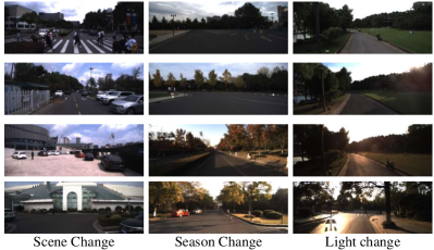
Figure 7: The images captured by the data collection vehicle at the same location but at different times.

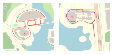
Figure 8: Partial demonstration of the data collection vehicle’s acquisition trajectories.

V System Evaluation Metric

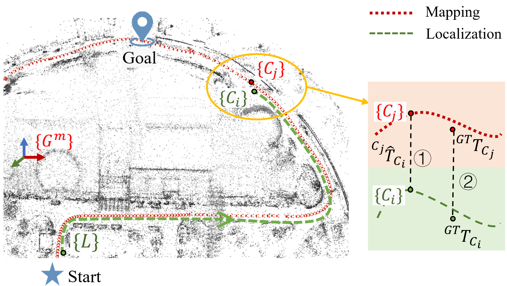
Figure 9: Illustration of the control error components in robot control example. The task is to navigate the robot from the start point to the goal in the $m$-th pre-built map frame. During the robot’s navigation process, take timestamp $i$ as an example, the error analysis between $C_{i}$ and the retrieved map frame $C_{j}$ is highlighted in the bottom right corner.

In this section we discuss how to evaluate the accuracy of trajectories obtained in the VILO. Let’s take an example of a real-world application scenario of VILO, which is a robot navigation scenario.

Real world robot navigation example. As shown in Fig. 9, for the task of navigating a robot from the start point to a goal, we first load a pre-built map covering the current area (in the example, this is the $m$-th map), and send the coordinate of the goal in the map’s frame $\{G^{m}\}$ to the robot. Subsequently, we execute the initialization module to align the robot’s starting point, i.e., the local frame $\{L\}$, with the map frame $\{G^{m}\}$, obtaining the estimated value of ${}^{G^{m}}\hat{\mathbf{T}}_{L}$. Then the map-based localization module is executed, which receives the data association between the robot and the map to obtain the current robot’s pose relative to the map frame in real time. Specifically, at time $i$, by matching the current camera image of $C_{i}$ with the corresponding map image of $C_{j}$ retrieved from the map, the filtered 2D-3D correspondences are sent to the localization module as map observations for state updating. Then the estimated pose of current robot ${}^{G^{m}}\hat{\mathbf{T}}_{C_{i}}$ can be used as position feedback to the robot’s control loop, guiding the robot towards the goal.

Localization error analysis. Analyzing the robot navigation process described above, it can be seen that the estimation accuracy of ${}^{G^{m}}\hat{\mathbf{T}}_{C_{i}}$ directly reflects the actual localization error of the robot. However, in practical applications, the success time of initialization varies with different methods. In some challenging scenarios with long-term changes, successful alignment with the map might not be achieved throughout the entire process. This results in different lengths of localization trajectories (i.e., sets of ${}^{G^{m}}\hat{\mathbf{T}}_{C_{i}}$) obtained by different methods, making it impossible to conduct a fair quantitative comparison.

To address this issue, we propose a new evaluation scheme that decouples the estimation of ${}^{G^{m}}\hat{\mathbf{T}}_{C_{i}}$ from the initialization time. Specifically, we introduce an alignment process that transforms the goal in the $\{G^{m}\}$ frame to the local frame $\{L\}$. This transformation can theoretically be completed automatically by initialization. However, to ensure that the initialization times are consistent across all methods, we manually complete this transformation in the first timestamp. Following this, the next step is to evaluate accuracy of the robot trajectory from the starting point to the goal in the $\{L\}$ frame. Thus, the entire evaluation process is divided into two stages: measuring the error of ${}^{G^{m}}\hat{\mathbf{T}}_{L}$ obtained during the initialization phase and, after manual alignment, the trajectory error of ${}^{L}\hat{\mathbf{T}}_{C_{i}}$. The first process is related to both the accuracy of the map construction and the matching between the robot and the map. In summary, the robot localization error consists of the following components:

• Mapping error. The pre-built map itself contains inherent errors, including the pose error of map keyframes and the error of map points triangulated from these keyframes.

• Matching error. In the process described above, matching error occurs in two stages: one during the initialization phase, and the other during the online matching between the robot and the map.

• Local-based trajectory error. This error refers to the accuracy of the robot trajectory in local frame after manual alignment at the first timestamp.

• Map-based trajectory error. This error refers to directly measuring the error of ${}^{G^{m}}\hat{\mathbf{T}}_{C_{i}}$, which is a comprehensive reflection of the three aforementioned errors. In simple scenarios where all methods can achieve successful localization quickly, this error can be directly used to compare localization accuracy.

Due to the distinct functionalities of the four error components, it is challenging to measure them using a single standard. Therefore, we conduct independent evaluations for each component. In the following section, we will elaborate on the measurement methods for different components.

V-A Mapping accuracy evaluation

V-A1 mapping accuracy of keyframes

Firstly, we consider the accuracy of the map keyframes. We use one of the most popular accuracy metrics for trajectory measuring, ATE, which assesses global consistency by comparing the absolute distances between the estimated trajectory and the ground truth trajectory. When comparing ATE, it is common to first align the trajectories of the two frames and then calculate the root mean square error of the differences at each time point. Thus, the mapping accuracy of keyframes is measured as:

$${E}_{mapping}^{k}=\;\sqrt{\frac{1}{N_{1}}\sum_{i=1}^{N_{1}}\|\mathbf{E}_{i}\|^{2}}$$ (28)

where $\|\cdot\|$ denotes the Euclidean distance, and $\mathbf{E}_{i}$ is the position error of two aligned points, which is defined as:

$$\mathbf{E}_{i}={{}^{GT}\mathbf{F}_{i}}-{{}^{GT}\mathbf{T}_{G^{m}}}\;^{G^{m}}\mathbf{F}_{i}$$ (29)

where ${}^{GT}\mathbf{p}_{i}$ and ${}^{G^{m}}\mathbf{p}_{i}$ is the position of ground truth and mapping trajectory at time $i$ ($i=1,\cdots,N_{1}$). ${{}^{GT}\mathbf{T}_{G^{m}}}$ is the rigid-body transformation matrix obtained by aligning the ground truth with the evaluated mapping trajectory using least squares method. Note that for simplification, we denote

$${{}^{A}\mathbf{T}_{B}}\mathbf{F}\triangleq\;^{A}\mathbf{R}_{B}\mathbf{F}+^{A}\mathbf{t}_{B}$$ (30)

V-A2 mapping accuracy of points

Due to the lack of a clear correspondence between map points and ground truth, we align the constructed map with the ground truth map using the Iterative Closest Point (ICP) method, and then use the ICP error as the indicator to measure the accuracy of map points. The ground truth and reconstructed map can be regarded as two set of points $\mathbf{M}$ and $\mathbf{Q}$, where each point in $\mathbf{M}$, the closest point in $\mathbf{Q}$ is identified as its corresponding point. $\mathbf{m}_{j}$ and $\mathbf{q}_{j}$ is the $j$-th corresponding point in $\mathbf{M}$ and $\mathbf{Q}$ ($j=1,\cdots,N_{2}$). Hence, the definition of mapping accuracy of map points is:

$${E}_{mapping}^{p}=\;\sqrt{\frac{1}{N_{2}}\sum_{j=1}^{N_{2}}\|\mathbf{m}_{j}-\mathbf{q}_{j}\|^{2}}$$ (31)

V-B Matching accuracy evaluation

The measurement method for both initial alignment and online matching is the same, involving the transformation between the robot’s current camera frame and the map camera frame in the map. We will use online matching as an example to illustrate this.

To measure the robot’s online matching error, specifically the error in the eatimated transformation ${}^{C_{j}}\hat{\mathbf{T}}_{C_{i}}$, we highlight this part for analysis in the bottom right corner of Fig. 9. The ground truth trajectory of mapping and localization is acquired from reliable external sensors. Based on timestamps, we can find the points with the closest timestamps on the ground truth map and the ground truth localization trajectory. ${}^{GT}\mathbf{T}_{C_{j}}$ represents the ground truth camera pose at time $j$ of the map, and ${}^{GT}\mathbf{T}_{C_{i}}$ represents the ground truth camera pose of the robot at the current time $i$. Then we can obtain the ground truth transformation between $\{C_{i}\}$ and $\{C_{j}\}$ as:

$${}^{{C_{j}}}\mathbf{T}_{{C}_{i}}=({{}^{GT}}\mathbf{T}_{C_{j}})^{-1}\;{{}^{GT}}\mathbf{T}_{C_{i}}$$ (32)

where $\mathbf{T}^{-1}$ means the inverse matrix of transformation matrix $\mathbf{T}$. And the estimated transformation ${}^{C_{j}}\hat{\mathbf{T}}_{C_{i}}$ (circle number 1 in Fig. 9) should be the same as ${}^{C_{j}}{\mathbf{T}}_{C_{i}}$ (circle number 2 in Fig. 9). Using the notation in (1), then we define the alignment accuracy as:

$${E}_{alignment}^{t}=\;\|^{{C_{j}}}\mathbf{t}_{{C}_{i}}-\;^{{C}_{j}}\hat{\mathbf{t}}_{{C}_{i}}\|$$ (33)

$${E}_{alignment}^{r}=\arccos(\frac{tr(^{{C}_{j}}\hat{\mathbf{R}}{{}^{\top}_{{C}_{i}}}^{{C_{j}}}\mathbf{R}_{{C}_{i}})-1}{2})$$ (34)

V-C Local-based trajectory accuracy

The third aspect to be evaluated is the accuracy of the robot’s trajectory after obtaining localization observations in the local frame. Some existing evaluation methods for trajectories, such as ATE and RPE, is non-causal which all utilize future information for evaluation. However, in practical applications, utilizing future information for feedback in control loop is impossible. The actual navigation planning at the current time is solely dependent on the localization error from the preceding time step, thus it can be regarded as a causal process.

V-C1 Non-causality of traditional methods

Firstly, both ATE and RPE require alignment of estimated trajectory and ground truth trajectory. However, their alignment actually depends on the entire trajectory, meaning that previous alignments require future trajectory information, which is non-causal. Secondly, when evaluating the current SLAM or VINS system, the output estimated trajectories undergo multiple loop corrections. Consequently, earlier trajectories are updated based on future loop closures. Therefore, a new evaluation metric is needed to evaluate the trajectory accuracy.

V-C2 Evaluation with causality

To solve the aforementioned second problem, we obtain an estimated trajectory that have not been post-processed denoted as $\{^{L}\mathbf{x}_{i}|^{L}\mathbf{x}_{i}\in SE_{3},i=1,\cdots,N_{3}\}$. $SE_{3}$ is the group of all rigid transformations in $\mathbb{R}^{3}$. And then we find the corresponding ground truth trajectory denoted as $\{^{GT}\mathbf{x}_{i}|^{GT}\mathbf{x}_{i}\in SE_{3},i=1,\cdots,N_{3}\}$. To solve the first problem, since we’ve already measured the alignment error, here, we manually align the first frame of the estimated trajectory with the first frame of the ground truth trajectory to ensure there are no alignment errors. Note that the alignment is performed in $SE_{3}$ and we only use the first frame to do alignment. Then we get ${{}^{GT}\mathbf{T}_{L}}$, which is the rigid-body transformation matrix obtained by aligning ${}^{L}\mathbf{x}_{1}$ with ${}^{GT}\mathbf{x}_{1}$.

After completing the steps above, we can then measure the trajectory errors $\{^{L}\mathbf{F}_{i}|i=2,\cdots,N_{3}\}$ for the remaining trajectory points in a manner similar to the ATE, as detailed below:

$${E}^{local}_{trajectory}=\sqrt{\frac{1}{N_{3}-1}\sum_{i=2}^{N_{3}}\|^{GT}\mathbf{F}_{i}-{{}^{GT}\mathbf{T}_{L}}^{L}\mathbf{F}_{i}\|^{2}}$$ (35)

V-D Map-based trajectory accuracy

When the localization scenario is relatively simple, i.e., there are no significant appearance or viewpoint changes, all methods can successfully complete initialization at the starting point. In this case, each method outputs localization estimation results in the map frame, denoted as $\{^{G_{m}}\mathbf{F}_{i}|i=1,\cdots,N_{3}\}$. We can directly compare the obtained trajectories with the ground truth trajectories. Note that alignment is not necessary because each method has already performed the alignment automatically. In fact, this evaluation metric is the ATE without alignment, as detailed below:

$${E}^{map}_{trajectory}=\sqrt{\frac{1}{N_{3}}\sum_{i=1}^{N_{3}}\|^{GT}\mathbf{F}_{i}-{{}^{G_{m}}\mathbf{F}_{i}}\|^{2}}$$ (36)

VI Experiments

To further evaluate the proposed algorithm, we conduct extensive experiments which can be divided into four parts. The first three parts evaluate the performance of the main modules in our system. The rest of the experiments test the accuracy and efficiency of the whole system.

We perform experiments maily on two datasets, including the newly collected ZJG dataset, and the publicly available Newer College dataset [41] (abbreviated as NC). The former has been described in detail above, and will not be repeated here for the sake of introduction. NC is a handheld multi-camera LiDAR inertial dataset covering a walking distance of 4.5 km and encompasses two distinct scenes: math and quad. The details of hardware design and dataset description is referred to [41].

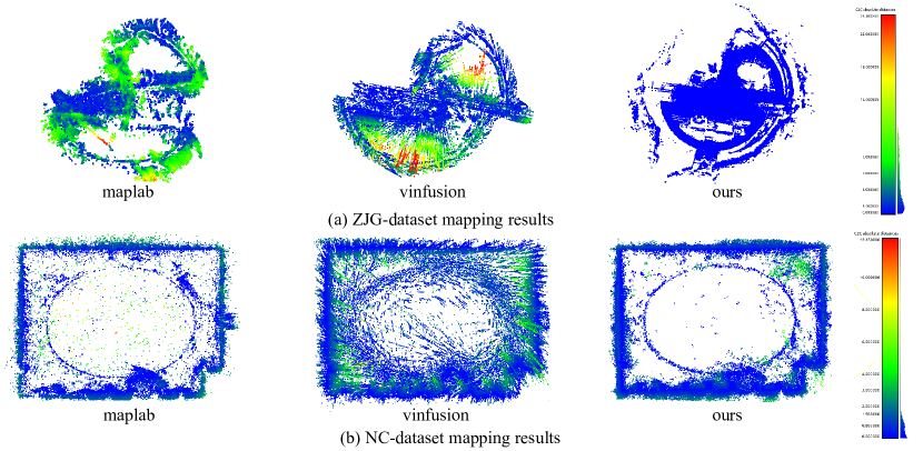
Figure 10: Map accuracy evaluation using ${E}_{mapping}^{p}$. The black point cloud is the ground truth, the colored point cloud corresponds to the result of different algorithms, and the color indicates the reconstruction error.

VI-A Mapping accuracy and robustness

To test the effectiveness of the proposed visual mapping module, we first evaluate the visual maps constructed by the visual mapping module described in Sec. III-C1-III-C2, using data from multi-camera and IMU sensors without relying on external sensor data. Then in Sec. VI-A2, we conduct experiment to demonstrate the impact of integrating external sensors on the accuracy of visual map construction. Also some ablation test results can be refer to the appendix.pdf in https://github.com/zoeylove/Multi-cam-Multi-map-VILO/tree/main.

TABLE VI: Mapping accuracy comparison results of each algorithm in ZJG and NC dataset.

Algorithm	ZJG-qsdjt-0924		NC-quad-easy
	mean	std	mean	std
OpenVINS	14.05	8.17	1.59	0.59
Maplab	20.64	6.69	1.25	0.43
Vins-fusion	1.98	0.37	0.45	0.14
Ours	1.55	0.61	0.31	0.12

VI-A1 Accuracy verification

In this section, we compare the reconstruction results using our method with other open source algorithms with mapping modules, to verify the advancedness of the algorithm. We test this on the NC dataset and ZJG dataset separately.

Quantitative comparison. The ground truth map for the NC and ZJG dataset are obtained by Leica BLK360, a survey-grade 3D imaging laser scanner, and results obtained from the LiDAR-inertial odometry algorithm [44]. After removing some outlier points by statistical outlier filter, we evaluate reconstruction results of each algorithm with the ground truth using ${E}_{mapping}^{p}$ metric in (31) and visualized the matching error for each point, as depicted in Fig. 10. The comparison highlights that our method achieves higher reconstruction accuracy than both Maplab and VINS-Fusion.

Qualitative comparison. To further evaluate the reconstruction accuracy visually, we perform a dense reconstruction based on the sparse results obtained from the earlier quantitative comparison. As illustrated in Fig. 12, the dense maps generated by our method closely match the actual camera-captured images, and the objects within these images have well-defined contours. This demonstrates the effectiveness of our dense reconstruction approach.

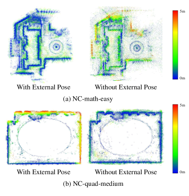
Figure 11: Mapping accuracy comparison results of whether or not to use external pose.

VI-A2 Comparison of different mapping method

In order to compare the impact of using an external pose on the accuracy of mapping building and subsequent localization applications, we conduct mapping building and localization comparison experiments using two scenarios, math-easy and quad-medium, on the NC dataset. We use the LiDAR in the dataset to run the open source LiDAR inertial odometry algorithm method FAST-LIO [45] to obtain external pose observations. The results of mapping accuracy comparison are shown in Fig.11, where math-easy has a much larger scene area than quad-medium. It can be seen that the introduction of an external pose can significantly improve the accuracy of the mapping in large-scale reconstruction task (NC-math-easy scene).

Next we perform our localization algorithm with maps constructed in different ways, the result is shown in Table VII. It can be seen that the introduction of external pose observation can greatly improve the localization accuracy in the case of a large map scene (NC-math), but the improvement is not obvious in the case of a small map scene (NC-quad).

TABLE VII: The translation part (m) of local-based trajectory error of different maps.

	With external pose		Without external pose
	mean	std	mean	std
NC-math-medium	1.01	0.44	1.69	0.86
NC-math-hard	3.76	1.75	4.12	2.01
NC-quad-easy	0.91	0.39	0.96	0.49
NC-quad-hard	1.14	0.44	1.15	0.45

VI-B Matching accuracy and robustness

VI-B1 Deterministic initialization evaluation

Robust, accurate, and reliable initialization is crucial for the actual execution of robots. Therefore, we will next focus on validating the reliability brought by the deterministic convergence of the proposed initialization method. The comparative method is the proposed probabilistic convergence method used in online matching module, 2P RANSAC, with the default iteration count set to 100. To highlight the probabilistic convergence characteristic of the RANSAC method, we also compare its variant by increasing the iteration count to 10,000 to enhance the probability of achieving optimal performance, denoted as 2P10K. For a quantitative measure of convergence, we compare the variance of the localization results. We conduct experiments on some selected typical cases in YQ dataset to evaluate the convergence of our proposed initialization method, following [46]. For each selected case, we execute each method 100 times to gather statistical results, which include the standard deviation, translation error, rotation error, and computation time. Note that the translation and rotation error are computed using the alignment evaluation metric in (33) and (34). The results, presented in Table VIII, indicate that the 2P10K method demonstrates better localization accuracy and lower variation, primarily due to its sampling variance. However, this method requires significantly more computation time to achieve better repeatability. In contrast, our proposed method not only achieves superior accuracy and perfect repeatability but also maintains reasonable time consumption. This performance advantage is attributed to the theoretical guarantee of deterministic global convergence provided by our method, making it more reliable and robust for practical applications.

TABLE VIII: Deterministic initialization performance.

ExpID	$N/\omega$	Method	$\triangle T$ (m)	$\sigma T$ (m)	$\triangle R$ (°)	$\sigma R$ (°)	Time (s)
01	26 / 0.82	2P	0.773	0.474	1.644	0.633	0.074
		2P10K	0.293	0.002	0.892	0.001	4.324
		Ours	0.154	0.000	0.498	0.000	0.100
02	68 / 0.78	2P	0.243	0.033	0.295	0.041	0.080
		2P10K	0.263	0.000	0.269	0.000	6.187
		Ours	0.049	0.000	0.267	0.000	0.320
03	15 / 0.47	2P	0.583	0.554	1.422	1.725	0.064
		2P10K	0.205	0.000	0.251	0.000	6.325
		Ours	0.187	0.000	0.130	0.000	0.080
04	49 / 0.65	2P	0.397	0.208	0.891	0.549	0.071
		2P10K	0.335	0.003	0.785	0.011	4.855
		Ours	0.283	0.000	0.596	0.000	0.150
05	82 / 0.72	2P	0.106	0.077	0.335	0.102	0.084
		2P10K	0.095	0.020	0.390	0.024	5.954
		Ours	0.045	0.000	0.320	0.000	0.420
06	138 / 0.38	2P	0.205	0.364	0.478	0.842	0.080
		2P10K	0.210	0.151	0.468	0.033	6.097
		Ours	0.125	0.000	0.390	0.000	0.680

• $N$ denotes the number of features, $\omega$ is the inlier rate and $\sigma$ is the standard deviation.

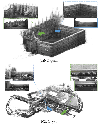
Figure 12: Dense reconstruction result using our method. Different colored arrows indicate different directions of observation. The dashed box shows the result of the dense reconstruction as viewed from the arrow of the corresponding color, and the solid box shows the corresponding real-world scene.

TABLE IX: Success rate comparison of mono-camera and multi-camera algorithms using matching error metric under different thresholds.

Task	session	YQ-2017-0827	YQ-2017-0828	YQ-2018-0129	NC-quad-hard	NC-math-hard
	m deg	0.25 / 0.5 / 1.0 / 5.0 2.0 / 5.0 / 8.0 / 10.0	0.25 / 0.5 / 1.0 / 5.0 2.0 / 5.0 / 8.0 / 10.0	0.25 / 0.5 / 1.0 / 5.0 2.0 / 5.0 / 8.0 / 10.0	0.25 / 0.5 / 1.0 / 5.0 2.0 / 5.0 / 8.0 / 10.0	0.25 / 0.5 / 1.0 / 5.0 2.0 / 5.0 / 8.0 / 10.0
Mono	P3P	15.6 / 28.6 / 38.2 / 49.4	16.2 / 32.1 / 39.1 / 47.1	09.2 / 18.3 / 27.8 / 45.2	2.75 / 10.56 / 26.68 / 55.13	2.05 / 10.36 / 30.64 / 74.83
	EPnP	15.9 / 29.2 / 38.6 / 50.7	17.8 / 33.0 / 39.6 / 47.6	09.8 / 20.7 / 28.8 / 45.6	2.66 / 10.96 / 28.50 / 54.86	2.43 / 10.74 / 32.35 / 74.21
	UPnP	19.2 / 33.1 / 39.2 / 51.8	19.6 / 34.3 / 38.2 / 47.4	10.4 / 21.3 / 28.2 / 46.8	2.62 / 10.52 / 27.08 / 54.86	1.95 / 10.50 / 30.71 / 74.66
	2P	21.9 / 33.8 / 41.0 / 54.6	20.9 / 31.9 / 37.1 / 44.3	13.9 / 24.4 / 33.5 / 53.5	8.17 / 21.66 / 39.37 / 57.08	5.51 / 19.66 / 44.63 / 80.03
Multi	GP3P	22.9 / 36.5 / 42.8 / 54.3	22.6 / 36.8 / 42.7 / 52.2	15.2 / 22.1 / 31.0 / 53.5	10.46 / 26.95 / 45.74 / 60.46	7.66 / 24.08 / 52.80 / 88.78
	GPnP	21.1 / 35.5 / 41.4 / 52.4	22.9 / 34.8 / 41.3 / 50.2	14.3 / 21.8 / 30.2 / 52.0	10.11 / 23.40 / 41.13 / 61.17	6.97 / 25.99 / 54.45 / 89.33
	MC2P	23.0 / 37.1 / 45.6 / 55.8	23.9 / 36.6 / 43.2 / 51.7	15.3 / 26.4 / 37.2 / 57.6	12.41 / 27.48 / 46.81 / 61.17	9.71 / 26.27 / 55.13 / 90.42

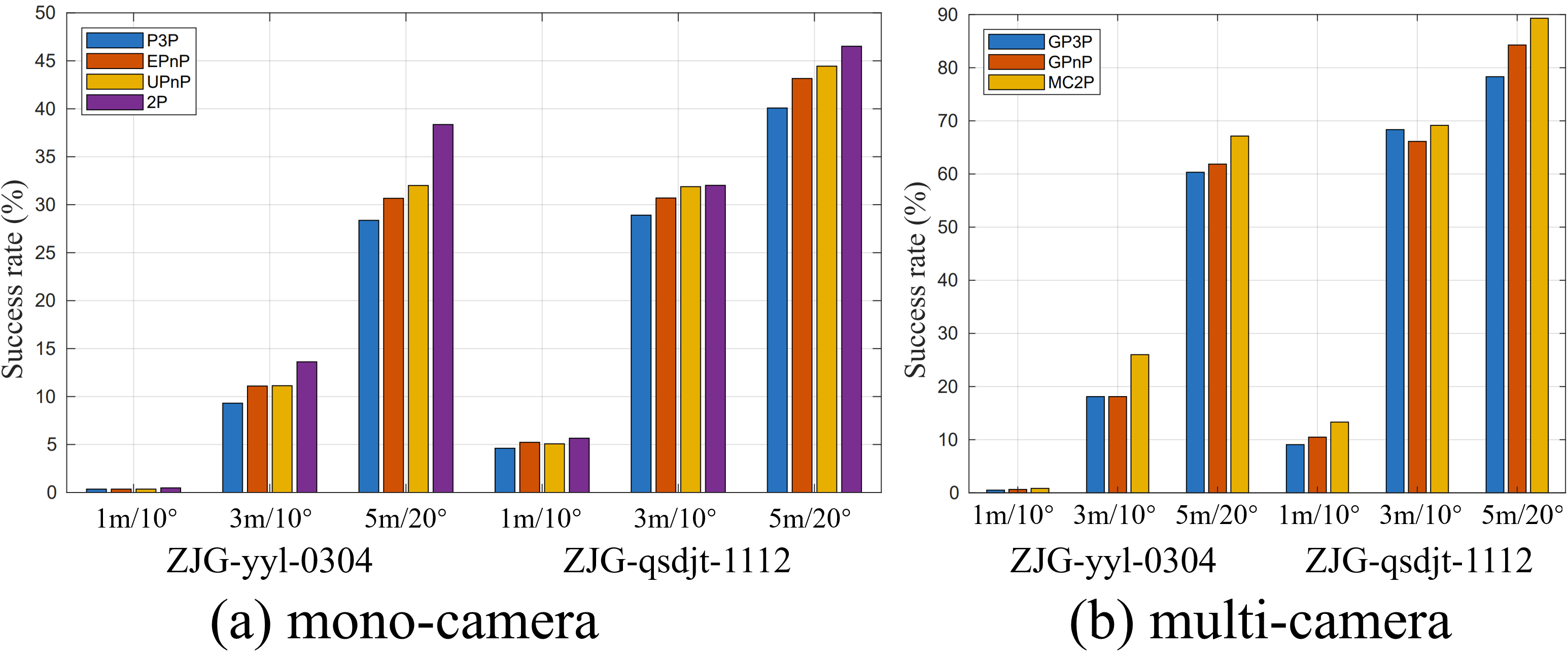
Figure 13: Success rate comparison on ZJG dataset using matching error metric under different thresholds.

VI-B2 Outlier rejection in online matching

After initialization, we perform online matching of keyframes and map images to obtain map-based observations. Specifically, for each retrieved image pairs matched by NetVLAD[47], we perform feature extraction and matching using SuperPoint [48]+LightGlue[49] and compare outlier rejection performance of different monocular and multi-camera pose estimation algorithms. For mono-camera pose estimation with a query image, we aggregate feature matches from the top5 retrieved map images to obtain the 2D-3D correspondence set. Then the RANSAC framework is employed for outlier rejection using different absolute pose estimation solutions for model estimation, including the proposed 2P minimal solution, the widely used classic P3P[50], EPnP[51] and UPnP[52] solutions. Then we compute the pose estimation error using the alignment evaluation metric in (33) and (34) to measure the feature matching accuracy and count the success rate within different error thresholds to evaluate the robustness. For multi-camera pose estimation, we also aggregate feature matches from the top5 retrieved map images for each query camera and perform RANSAC using different multi-camera solutions including the proposed MC2P, the genreal 6DoF solutions GP3P[53] and GPnP[53]. The success rate comparison result is shown in Table IX for YQ and NC datsets and Fig. 13 for ZJG dataset.

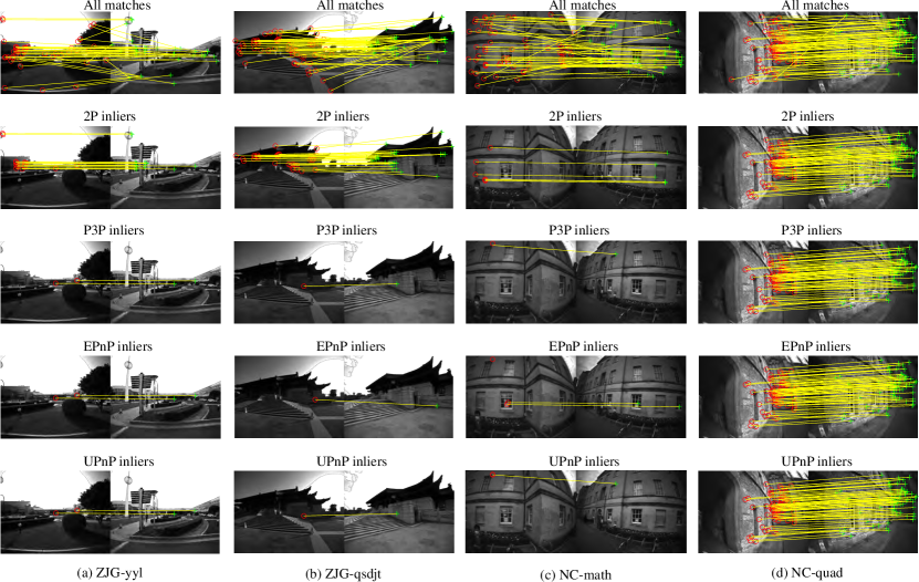
Figure 14: Illustration of matching inliers identified by different algorithms.

Minimal solutions. As expected, multi-camera algorithms show significant improvements over mono-camera algorithms. Particularly, when applying the proposed MC2P algorithm on the NC dataset with a high-precision localization threshold of 0.25m, the success rate is 4.5 times higher than the monocular P3P approach. The multi-camera algorithm exhibits more notable enhancements on the NC dataset than on the YQ dataset. This is because NC scenes are circular and small-scale, where each perspective in a multi-camera setup can capture many effective scenes. Additionally, the proposed 2P and MC2P minimal solutions, derived from 4DoF pose estimation modeling, achieved better performance than other comparative methods in most scenarios, especially in those with long-term appearance changes and significant viewpoint variations. For instance, the YQ scene from 2018-01-29, compared to the summer mapping scene, is in a post-snow winter with changes like fallen leaves and snow-covered roads and buildings. NC scenes, due to their circular motion pattern, exhibit large viewpoint changes, as shown in Fig. 14. Such long-term and viewpoint changes directly reduce feature extraction repeatability, leading to fewer feature matches and an increased proportion of mismatches. Applying the proposed minimal solution methods, which require fewer features for pose estimation, significantly increases the success rate of selecting inliers for estimation based on RANSAC’s probabilistic analysis, thereby notably enhancing localization robustness.

Similarly, in the ZJG dataset, the significant viewpoint changes lead to a high proportion of mismatches in feature matching. Additionally, since the features are distributed in scenes farther from the camera, the accuracy of depth estimation is limited, resulting in lower precision in pose estimation and consequently a lower success rate for high-precision localization. Nevertheless, the proposed method still achieves better robustness than the comparative methods that require more features, including both mono-camera and multi-camera algorithms, which validates the robustness of our method in changing environment.

Conversely, in scenarios without significant long-term changes, such as in YQ-2017-0828, where the data collection time is similar to the map collection time and both occur in the afternoon with similar lighting conditions, the performance of the proposed method is slightly inferior to the comparative methods. This is because, in such scenarios, feature matching tends to be more accurate due to the abundance of features and a high proportion of correct matches. Therefore, methods optimizing 6DoF, including both pitch and roll angles, achieve better accuracy than the proposed 4DoF method.

Case study. We select representative cases from the ZJG and NC datasets to explicitly illustrate feature matching performance, with results shown in Fig. 14. The principle of the minimal solution for multi-camera algorithms is similar to that for mono-camera. For ease of comparison, we demonstrate the matching situation with the mono-camera algorithms. From Fig. 14 (a), it is evident that ZJG-yyl is a typical large-scale unstructured scene, lacking significant and distinctive visual features. This results in a low number of feature matches. Additionally, the scene shown exhibits large viewpoint changes, further reducing the number of repeated observations. Consequently, the number of feature matches is extremely low, and the proportion of outliers is very high. Due to the nature of the proposed 2P algorithm, during RANSAC iterations, only two point correspondences are needed to compute the absolute pose of the camera, whereas comparative methods like P3P and EPnP require 3-4 pairs. From a statistical probability perspective, this significantly increases the likelihood of selecting inliers for pose estimation. This means that the success rate of pose estimation can be significantly improved. Based on the estimated pose, correct feature matches can be filtered out from the matches. In contrast, other methods fail in pose estimation.

Fig. 14 (b) to (c) show cases with a high proportion of feature matching outliers due to extreme changes in viewpoint. However, in environments without long-term appearance changes and with clear structural features, where feature matching is good, as shown in Fig. 14 (d), all methods can filter out a large number of correct feature matches.

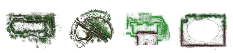
Figure 15: Multi-map experiment result, which shows the merged result of final estimated extrinsic by the proposed system. The scenes in order from left to right are ZJG-qsdjt, ZJG-yyl, NC-math and NC-quad.

TABLE X: The translation part (m) of local-based trajectory error under different number of maps.

Scene	map1		map2		2 maps
	mean	std	mean	std	mean	std
ZJG-yyl-0304	2.24	0.68	3.50	2.26	2.23	0.63
ZJG-qsdjt-1112	1.98	1.26	2.19	1.14	1.85	1.06
NC-math-hard	1.22	0.42	0.44	0.23	0.47	0.19
NC-quad-hard	0.22	0.18	0.17	0.09	0.16	0.07

VI-C Localization accuracy and robustness

In this section we verify the effectiveness of our proposed localization module and the effect of different configurations on the algorithm. Some ablation test results can be refer to the appendix.pdf in https://github.com/zoeylove/Multi-cam-Multi-map-VILO/tree/main.

VI-C1 Evaluation of muli-map configuration

Since our algorithm supports multi-map modes both with overlap and non-overlap , we set up the configuration with two separate multi-map configurations without overlap (NC dataset) and with overlap (ZJG-dataset). The specific distribution of map observations is shown in Fig. 15. For each scenario we have selected two sub-maps, and the individual localization results and fused localization results for each map are shown in Table X. The results show that under different map configurations, the localization accuracy of multiple maps is better than that of a single map, while the fluctuation amplitude of localization is reduced. It can be seen that our method can effectively resist the interference caused by bad map information when dealing with multi-map information.

In order to further illustrate the advantages of our algorithm when dealing with multi-map information, we also perform qualitative analyses. Since our algorithm estimates the extrinsic between the frame of each map and VIO simultaneously during the localization, we use the results of the final estimate of the extrinsic to transform the different maps to a uniform frame (i.e., the frame of the current VIO). The results are shown in Fig. 15. Brown and green represent Map 1 and Map 2, respectively. It is observed that the spliced trajectories exhibit minimal branching, and the edge contours of the sparse maps remain distinct post-splicing. This qualitative assessment suggests that the accuracy of the extrinsic parameters between multiple maps frames and the VIO frames, as estimated by the proposed system, is high.

TABLE XI: The translation part (m) of local-based trajectory accuracy of each method operating on various challenge environments.

	VILO(ours)		VINS-Fusion		ORB-SLAM3
	mean	std	mean	std	mean	std
quad-easy	1.24	0.59	1.81	0.47	2.97	1.22
quad-hard	1.58	0.79	1.06	0.85	fail	fail
math-hard	3.94	1.76	fail	fail	34.05	14.76
math-medium	1.18	0.60	1.58	0.66	13.59	6.11
yyl-1022	2.78	1.58	fail	fail	7.61	3.67
yyl-1112	4.23	2.08	4.84	2.19	4.29	1.80
qsdjt-1022	7.67	3.41	14.03	6.56	4.55	3.08
qsdjt-0224	15.17	3.71	24.74	25.06	fail	fail
Average	4.72	1.82	8.01	5.97	11.18	5.11

• fail indicates great drift in the odometer during the movement.

TABLE XII: The translation part (m) of map-based trajectory error of each method operating on Euroc dataset.

	VILO(ours)		ORB-SLAM3		VINS-Fusion		Maplab
	mean	std	mean	std	mean	std	mean	std
MH02	0.18	0.08	1.82	2.25	0.38	0.11	1.45	0.61
MH03	0.29	0.09	0.21	0.38	0.36	0.14	0.92	0.39
MH04	0.43	0.16	fail	fail	0.53	0.11	1.78	0.58
MH05	0.59	0.34	fail	fail	0.56	0.17	2.06	0.74
V102	0.18	0.05	0.49	0.89	0.19	0.04	0.06	0.04
V103	0.24	0.08	0.27	0.69	2.82	0.72	0.10	0.04
V202	0.12	0.05	0.32	0.79	0.73	0.40	0.08	0.07
V203	0.25	0.1	fail	fail	1.03	0.59	0.21	0.09
Average	0.29	0.12	0.62	1.0	0.83	0.29	0.83	0.32

• fail indicates that there is no successful localization during the movement.

VI-D Real-time system evaluation

After evaluating the mapping accuracy and relative localization accuracy, we assess the real-time trajectory accuracy of the entire system. We compare our algorithm with some current state-of-the-art visual slam algorithms that support reusing map for localization. In order to compare real-time performance, we recorded the real-time outputs with optimized back-end algorithms, i.e., ORB-SLAM3 and VINS-Fusion, with loop-closure optimization turned off.

We first test on the NC and ZJG dataset to evaluate the local-based trajectory error. We use the external pose obtained from the Fast-LIO to construct a localization map in our method. Other methods use their respective methods to build localization map. Since maplab’s front-end (ROVIO) fails in most outdoor scenarios, it is not considered in the comparison methodology. Besides, since ORB-SLAM3 will match the current frame with the merged map when the localization is successful, the odometry will generate a mutation, and in order to avoid the impact of this mutation on the comparison results, we only use its odometry result after the localization is successful. The results are shown in Table XI. The first four are scenarios from the NC dataset, and the naming convention is “location-difficulty”. The rest are scenarios in the ZJG dataset, and the naming convention is “location-time”.

Then we test the map-based trajectory accuracy on Euroc dataset [38] that focuses on indoor scenes. We use the least squares algorithm to align the trajectories of the maps constructed by the respective algorithms with the same session ground truth respectively, and after obtaining different transformation matrices, we transform the ground truth trajectories of the corresponding localization sessions into the constructed map coordinate system through the transformation matrix. The results are shown in Table XII. We use the data of MH01, V101 and V201 to build the localization maps with their respective algorithms to the sessions starting with MH, V1 and V2 to the corresponding algorithms. As for our algorithms, we use the mapping method withourt external pose data.

As can be seen from the table, our method has the highest average trajectory accuracy and smallest error fluctuation on both local-based trajectory and map-based trajectory accuracy comparison test. This shows that our method have the best localization results in real navigation applications. Since the euroc dataset is an indoor scene dataset, which is less challenging for different localization algorithms and is not equipped with a multi-camera sensor, the advantages of our approach are not as great as they are on the ZJG and NC datasets.

Besides, the other algorithms vary widely in their localization results in different scenes because of the different spatial sizes of the scenes beginning with V1 and V2 and the scenes beginning with MH. In comparison, our algorithm is better adapted to the scene, so the overall localization accuracy does not fluctuate much with the scene.

VII Conclusion

We present a multi-cam and multi-map visual inertial localization system, supporting long-term navigation tasks for robots. Besides, we thoroughly investigate the impact of robot localization on navigation task and propose A comprehensive method for evaluating the accuracy of localization systems for practical navigation applications. In addition, we provide a dataset collected in a campus scene used to validate the algorithm, containing the same location under different illumination and seasons. A variety of experiments have demonstrated that our method can achieve higher real-time localization accuracy in both indoor and outdoor scenarios. Our system is open source, which facilitates research on robot navigation applications in academia and industry.

References

- [1] G. Huang, “Visual-inertial navigation: A concise review,” in 2019 international conference on robotics and automation (ICRA). IEEE, 2019, pp. 9572–9582.
- [2] Z. Huai and G. Huang, “A consistent parallel estimation framework for visual-inertial slam,” IEEE Transactions on Robotics, 2024.
- [3] Y. Yang, P. Geneva, X. Zuo, and G. Huang, “Online self-calibration for visual-inertial navigation: Models, analysis, and degeneracy,” IEEE Transactions on Robotics, vol. 39, no. 5, pp. 3479–3498, 2023.
- [4] K. Eckenhoff, P. Geneva, and G. Huang, “Mimc-vins: A versatile and resilient multi-imu multi-camera visual-inertial navigation system,” IEEE Transactions on Robotics, vol. 37, no. 5, pp. 1360–1380, 2021.
- [5] T. Qin, P. Li, and S. Shen, “Vins-mono: A robust and versatile monocular visual-inertial state estimator,” IEEE Transactions on Robotics, vol. 34, no. 4, pp. 1004–1020, 2018.
- [6] C. Campos, R. Elvira, J. J. G. Rodríguez, J. M. Montiel, and J. D. Tardós, “Orb-slam3: An accurate open-source library for visual, visual–inertial, and multimap slam,” IEEE Transactions on Robotics, vol. 37, no. 6, pp. 1874–1890, 2021.
- [7] A. Cramariuc, L. Bernreiter, F. Tschopp, M. Fehr, V. Reijgwart, J. Nieto, R. Siegwart, and C. Cadena, “maplab 2.0–a modular and multi-modal mapping framework,” IEEE Robotics and Automation Letters, vol. 8, no. 2, pp. 520–527, 2022.
- [8] M. A. Fischler and R. C. Bolles, “Random sample consensus: a paradigm for model fitting with applications to image analysis and automated cartography,” Communications of the ACM, vol. 24, no. 6, pp. 381–395, 1981.
- [9] M. Labbé and F. Michaud, “Rtab-map as an open-source lidar and visual simultaneous localization and mapping library for large-scale and long-term online operation,” Journal of field robotics, vol. 36, no. 2, pp. 416–446, 2019.
- [10] T. Qin and S. Shen, “Online temporal calibration for monocular visual-inertial systems,” in 2018 IEEE/RSJ International Conference on Intelligent Robots and Systems (IROS). IEEE, 2018, pp. 3662–3669.
- [11] A. Rosinol, M. Abate, Y. Chang, and L. Carlone, “Kimera: an open-source library for real-time metric-semantic localization and mapping,” in 2020 IEEE International Conference on Robotics and Automation (ICRA). IEEE, 2020, pp. 1689–1696.
- [12] S. Urban and S. Hinz, “Multicol-slam-a modular real-time multi-camera slam system,” arXiv preprint arXiv:1610.07336, 2016.
- [13] L. Zhang, D. Wisth, M. Camurri, and M. Fallon, “Balancing the budget: Feature selection and tracking for multi-camera visual-inertial odometry,” IEEE Robotics and Automation Letters, vol. 7, no. 2, pp. 1182–1189, 2021.
- [14] W. Zhang, S. Wang, X. Dong, R. Guo, and N. Haala, “Bamf-slam: Bundle adjusted multi-fisheye visual-inertial slam using recurrent field transforms,” arXiv preprint arXiv:2306.01173, 2023.
- [15] Y. Wang, Y. Ng, I. Sa, A. Parra, C. Rodriguez, T. J. Lin, and H. Li, “Mavis: Multi-camera augmented visual-inertial slam using se2 (3) based exact imu pre-integration,” arXiv preprint arXiv:2309.08142, 2023.
- [16] P. Geneva, K. Eckenhoff, W. Lee, Y. Yang, and G. Huang, “Openvins: A research platform for visual-inertial estimation,” in 2020 IEEE International Conference on Robotics and Automation (ICRA). IEEE, 2020, pp. 4666–4672.
- [17] Y. Yang, P. Geneva, K. Eckenhoff, and G. Huang, “Degenerate motion analysis for aided ins with online spatial and temporal sensor calibration,” IEEE Robotics and Automation Letters, vol. 4, no. 2, pp. 2070–2077, 2019.
- [18] C. Forster, L. Carlone, F. Dellaert, and D. Scaramuzza, “On-manifold preintegration for real-time visual–inertial odometry,” IEEE Transactions on Robotics, vol. 33, no. 1, pp. 1–21, 2016.
- [19] D. Gálvez-López and J. D. Tardos, “Bags of binary words for fast place recognition in image sequences,” IEEE Transactions on Robotics, vol. 28, no. 5, pp. 1188–1197, 2012.
- [20] T. Qin, P. Li, and S. Shen, “Vins-mono: A robust and versatile monocular visual-inertial state estimator,” IEEE Transactions on Robotics, vol. 34, no. 4, pp. 1004–1020, 2018.
- [21] T. Qin, J. Pan, S. Cao, and S. Shen, “A general optimization-based framework for local odometry estimation with multiple sensors,” 2019.
- [22] T. Shan, B. Englot, C. Ratti, and D. Rus, “Lvi-sam: Tightly-coupled lidar-visual-inertial odometry via smoothing and mapping,” in 2021 IEEE international conference on robotics and automation (ICRA). IEEE, 2021, pp. 5692–5698.
- [23] F. Han, S. Jia, Y. Jiao, W. Huang, Y. Wang, and R. Xiong, “Two-stage multi-camera constrain mapping pipeline for large-scale 3d reconstruction,” in 2023 42nd Chinese Control Conference (CCC). IEEE, 2023, pp. 4351–4356.
- [24] G. Carrera, A. Angeli, and A. J. Davison, “Slam-based automatic extrinsic calibration of a multi-camera rig,” in 2011 IEEE International Conference on Robotics and Automation. IEEE, 2011, pp. 2652–2659.
- [25] J. L. Schönberger and J.-M. Frahm, “Structure-from-motion revisited,” in Conference on Computer Vision and Pattern Recognition (CVPR), 2016.
- [26] J. L. Schönberger, E. Zheng, M. Pollefeys, and J.-M. Frahm, “Pixelwise view selection for unstructured multi-view stereo,” in European Conference on Computer Vision (ECCV), 2016.
- [27] M. A. Fischler and R. C. Bolles, “Random sample consensus: a paradigm for model fitting with applications to image analysis and automated cartography,” Communications of the ACM, vol. 24, no. 6, pp. 381–395, 1981.
- [28] S. Choi, T. Kim, and W. Yu, “Performance evaluation of ransac family,” Journal of Computer Vision, vol. 24, no. 3, pp. 271–300, 1997.
- [29] M. Brown, D. Windridge, and J.-Y. Guillemaut, “Globally optimal 2d-3d registration from points or lines without correspondences,” in Proceedings of the IEEE International Conference on Computer Vision, 2015, pp. 2111–2119.
- [30] D. Campbell, L. Petersson, L. Kneip, and H. Li, “Globally-optimal inlier set maximisation for simultaneous camera pose and feature correspondence,” in Proceedings of the IEEE International Conference on Computer Vision, 2017, pp. 1–10.
- [31] T.-J. Chin, Y. Heng Kee, A. Eriksson, and F. Neumann, “Guaranteed outlier removal with mixed integer linear programs,” in Proceedings of the IEEE Conference on Computer Vision and Pattern Recognition, 2016, pp. 5858–5866.
- [32] M. Li and A. I. Mourikis, “High-precision, consistent ekf-based visual-inertial odometry,” The International Journal of Robotics Research, vol. 32, no. 6, pp. 690–711, 2013.
- [33] Y. Jiao, Y. Wang, X. Ding, M. Wang, and R. Xiong, “Deterministic optimality for robust vehicle localization using visual measurements,” IEEE Transactions on Intelligent Transportation Systems, vol. 23, no. 6, pp. 5397–5410, 2021.
- [34] Y. Jiao, Y. Wang, X. Ding, B. Fu, S. Huang, and R. Xiong, “2-entity random sample consensus for robust visual localization: framework, methods, and verifications,” IEEE Transactions on Industrial Electronics, vol. 68, no. 5, pp. 4519–4528, 2020.
- [35] A. I. Mourikis and S. I. Roumeliotis, “A multi-state constraint kalman filter for vision-aided inertial navigation,” in Proceedings 2007 IEEE international conference on robotics and automation. IEEE, 2007, pp. 3565–3572.
- [36] Z. Zhang, Y. Jiao, S. Huang, R. Xiong, and Y. Wang, “Map-based visual-inertial localization: Consistency and complexity,” IEEE Robotics and Automation Letters, vol. 8, no. 3, pp. 1407–1414, 2023.
- [37] Z. Zhang, Y. Jiao, R. Xiong, and Y. Wang, “Fusing multiple isolated maps to visual inertial odometry online: A consistent filter,” IEEE Transactions on Automation Science and Engineering, 2023.
- [38] M. Burri, J. Nikolic, P. Gohl, T. Schneider, J. Rehder, S. Omari, M. W. Achtelik, and R. Siegwart, “The euroc micro aerial vehicle datasets,” The International Journal of Robotics Research, vol. 35, no. 10, pp. 1157–1163, 2016.
- [39] A. Geiger, P. Lenz, C. Stiller, and R. Urtasun, “Vision meets robotics: The kitti dataset,” The International Journal of Robotics Research, vol. 32, no. 11, pp. 1231–1237, 2013.
- [40] Y. Liao, J. Xie, and A. Geiger, “KITTI-360: A novel dataset and benchmarks for urban scene understanding in 2d and 3d,” Pattern Analysis and Machine Intelligence (PAMI), 2022.
- [41] L. Zhang, M. Camurri, D. Wisth, and M. Fallon, “Multi-camera lidar inertial extension to the newer college dataset,” arXiv preprint arXiv:2112.08854, 2021.
- [42] J. Yin, A. Li, T. Li, W. Yu, and D. Zou, “M2dgr: A multi-sensor and multi-scenario slam dataset for ground robots,” IEEE Robotics and Automation Letters, vol. 7, no. 2, pp. 2266–2273, 2022.
- [43] N. Carlevaris-Bianco, A. K. Ushani, and R. M. Eustice, “University of michigan north campus long-term vision and lidar dataset,” The International Journal of Robotics Research, vol. 35, no. 9, pp. 1023–1035, 2016.
- [44] W. Xu, Y. Cai, D. He, J. Lin, and F. Zhang, “Fast-lio2: Fast direct lidar-inertial odometry,” IEEE Transactions on Robotics, vol. 38, no. 4, pp. 2053–2073, 2022.
- [45] W. Xu and F. Zhang, “Fast-lio: A fast, robust lidar-inertial odometry package by tightly-coupled iterated kalman filter,” IEEE Robotics and Automation Letters, vol. 6, no. 2, pp. 3317–3324, 2021.
- [46] P. Speciale, D. Pani Paudel, M. R. Oswald, T. Kroeger, L. Van Gool, and M. Pollefeys, “Consensus maximization with linear matrix inequality constraints,” in Proceedings of the IEEE Conference on Computer Vision and Pattern Recognition, 2017, pp. 4941–4949.
- [47] R. Arandjelovic, P. Gronat, A. Torii, T. Pajdla, and J. Sivic, “Netvlad: Cnn architecture for weakly supervised place recognition,” in Proceedings of the IEEE conference on computer vision and pattern recognition, 2016, pp. 5297–5307.
- [48] D. DeTone, T. Malisiewicz, and A. Rabinovich, “Superpoint: Self-supervised interest point detection and description,” in Proceedings of the IEEE conference on computer vision and pattern recognition workshops, 2018, pp. 224–236.
- [49] P. Lindenberger, P.-E. Sarlin, and M. Pollefeys, “Lightglue: Local feature matching at light speed,” in Proceedings of the IEEE/CVF International Conference on Computer Vision, 2023, pp. 17 627–17 638.
- [50] X.-S. Gao, X.-R. Hou, J. Tang, and H.-F. Cheng, “Complete solution classification for the perspective-three-point problem,” IEEE transactions on pattern analysis and machine intelligence, vol. 25, no. 8, pp. 930–943, 2003.
- [51] V. Lepetit, F. Moreno-Noguer, and P. Fua, “Epnp: An accurate o (n) solution to the pnp problem,” International journal of computer vision, vol. 81, no. 2, p. 155, 2009.
- [52] L. Kneip, H. Li, and Y. Seo, “Upnp: An optimal o (n) solution to the absolute pose problem with universal applicability,” in European Conference on Computer Vision. Springer, 2014, pp. 127–142.
- [53] L. Kneip, P. Furgale, and R. Siegwart, “Using multi-camera systems in robotics: Efficient solutions to the npnp problem,” in 2013 IEEE International Conference on Robotics and Automation. IEEE, 2013, pp. 3770–3776.