General relativity and the double-zero eigenvalue

Abstract

For a given nonlinear system of dynamical equations, the set of all stable perturbations of the system, the ‘versal unfolding’, is fully determined by bifurcation theory. This leads to a complete depiction of all possible qualitatively different solutions and their metamorphoses into new topological forms, the versal families being dependent on a suitable number - the codimension - of independent parameters. In this paper, we introduce and elaborate on the idea that gravitational phenomena are bifurcation problems of finite codimension. We deploy gravitational bifurcations for five standard problems in general relativity, namely, the Friedmann models, the Oppenheimer-Snyder black hole, the issue of a focussing state associated with the evolution of congruences of causal geodesics in the context of cosmology and black holes, the crease flow on black hole event horizons, and the Friedmann-Lemaître equations. We also comment on more general emerging aspects of the application of bifurcation theory to problems involving the gravitational interaction, and the possible relations between gravitational versal unfoldings and those of the Maxwell, Dirac, and Schrödinger equations.

1 Introduction

There is a somewhat concealed feature of gravitational field equations and their possible reductions in specialized situations describing phenomena of interest in cosmology, black holes, and other areas in gravity research. It is shared for example by the Einstein equations, or by analogous ones in modified gravity or string theories, and also by ‘optical’ type systems describing the evolution of congruences of causal curves or higher-dimensional gravitating objects in spacetime. This feature can be well described both physically and mathematically by the statement that:

Gravitation is a bifurcation problem.

The main message of this paper is that gravitation is a structurally unstable phenomenon and must be treated using an approach where this feature does not disappear altogether in the process but persists. In particular, the observed cosmic structures could have never been formed and persisted had gravity been structurally stable. How then does gravitational instability in its various forms manifest itself as structural instability of the governing gravitational equations? How can one describe the latter in a mathematically precise yet physically consistent and plausible way? What are the main physical implications predicted by gravitational structural instability alone that could never have arisen had we treated the equations of a particular gravitational setup as being structurally stable?

Physically speaking, bifurcation theory may be defined as the study of structurally unstable (also called ‘dispersive’) phenomena, and while its precise nature as a mathematical theory is probably unfamiliar to, or perhaps even might be considered as peripheral at best by, experts in the field of gravitation, the purpose of this paper is rather to suggest that there is a fundamental link between gravity and bifurcation theory and explore this relation using methods of the singularity theory of functions.

Structural stability is a mathematically well-known concept of stability that refers to the stability of the laws themselves, that is to the dynamical equations governing the phenomena, as opposed to the stability of their specific solutions. However, it imposes very strong restrictions to the solutions describing different manifestations of the physical phenomena associated with these laws. For a system described by such equations, the spectrum of possible behaviours is restricted by the condition that any nearby system, i.e., any small perturbation of the system, behaves exactly as the original one [23]-[25].

This demand of structural stability on a given system leads to only three possible behaviours for any solution: stable, unstable, or saddle-like. That is, either there is nothing new, i.e., a solution rapidly dies out and the system returns to its unperturbed state, or diverges, ripping the system apart, or - as perhaps the worst alternative - a mixture of the two that results in an unstable saddle-like state. Consequently, such a system is in some sense always ‘trapped in itself’ being unable to pass to another, qualitatively different, state like for example one of those we observe around us (this will be made precise below).

There is a great difference between structurally stable and dispersive systems of dynamical equations [26], [27]. For our present purposes, a very characteristic manifestation of that difference is provided by the phenomenon of gravitational instability, as in the problem of cosmological structure formation where, albeit usually treated in the linear approximation [28]-[38], the universe was very smooth but has become very inhomogeneous on small scales as cosmological observations clearly suggest. The universe ‘settles down’ to a novel state which albeit a changing one does not suddenly disappear but ‘persists’ for a time comparable to the observed lifetime of the system.

In addition to the above, gravitational systems share two further properties which are in fact very akin to those of typical structurally unstable systems:

1. They possess parameters whose values are not really known exactly.

2. They are described by differential equations which are very sensitive to even very small changes or modifications of their defining terms.

The fluid parameter $\gamma$, or a cosmological constant are examples of the first property, while any randomly picked system of equations describing a gravity problem may be indicative of the second. Although a demand of structural stability is understandable as it implies that a property possessed by such a system is then physically very plausible, such a restriction imposed on an unstable system satisfying the two above conditions may lead to non-characteristic results attributed to the original equations and leave out other behaviours which might lie closer to the nature of the system’s instabilities.

Another related issue is what one really means by ‘stability’ in the unstable context of a structurally unstable system? How may one classify the various unstable modes available in a given gravitational problem described and governed by a structurally unstable set of dynamical equations? Such issues point to a further consideration of related questions. For example, how can one perturb a structurally unstable system? What is the possible range of such perturbations, and how are the solutions of the original system are being affected by the latter? What is the meaning of the phrase ‘small perturbation’ for a structurally unstable situation where there may be almost ignorable perturbations that have the ability to completely corrupt all orbits?

We shall return to these questions in the coming sections of this paper, where we shall introduce the approach of bifurcation theory to this problem. Basically, very roughly speaking, this approach to the problem of general gravitational instabilities dictates that: one must first recognise the kinds of degeneracy of the original system by bringing it in a ‘normal form’; secondly, embed the system of dynamical equations in a suitable larger parametric family customized to the given problem; and thirdly, prove that this family contains generically all possible stable perturbations of the original system. This is a long path but eventually becomes very rewarding. One acquires control over all degeneracies of the original system, now in a structurally stable framework where each unstable aspect persists, and one is in this way led to a spectrum of all possible behaviours associated with the original system.

In Section 2, we discuss the main differences between hyperbolic and nonhyperbolic systems, and in Section 3 we formulate the main problem addressed in this work and write down the central objectives in the search of gravitational bifurcations. Section 4 gives a brief exposition of the main methods of bifurcation theory. In Section 5, we study the picture which emerges from an application of these methods to some of the most basic and well-studied gravity problems in general relativity, cosmology, and black holes. In the last Section, we discuss more general issues which emerge from gravitational bifurcations.

This work is based on the results of Refs. [19]-[22], however, we skip all details of the long arguments and calculations needed to prove many of the statements made in those references and referred to here. After reading the present paper, we hope that the reader will be sufficiently motivated to at least look at some of the proofs in those references.

2 Hyperbolic vs. dispersive systems

2.1 General comments

Besides in the theory of small fluctuations mentioned above, an essentially ‘hyperbolic’ approach based on the concept of structural stability is as a rule the one used in other dynamical treatments of gravity problems, cf. e.g., [39]-[41] and refs. therein, and has its roots in the standard theory of (hyperbolic) dynamical systems [23]-[25]. As is well-known this practice leads to systems with (usually complicated) hyperbolic equilibria, and so imposes two very important conditions on the gravity systems studied in this way: firstly, near such equilibria they become topologically equivalent to their linear parts, and secondly, ‘nearby’ nonlinear systems behave like their unperturbed counterparts.

We shall consider structurally unstable systems only and not follow the more or less common approach of restricting the parameters present in a gravity problem to suitable intervals, and then treat a possibly dispersive system as being structurally stable. Our approach has a very high applicability not only in cosmology but in other areas as well (for a description of possible cosmological areas of application of these ideas, cf. e.g., [42]).

To motivate our approach to gravitational bifurcation theory employed in following Sections, let us recall the difference between a hyperbolic and a non-hyperbolic system (a hyperbolic system is one whose all equilibria are hyperbolic). This difference arises in two ways: while equilibria in a hyperbolic system are always isolated and the behaviour of solutions near them is qualitatively the same as that of their linear parts, dispersive systems exhibit bifurcating behaviour and as a rule comprise multiple solutions intertwined with dramatic changes in the behaviour, while their global dynamics is restricted to only those dimensions which correspond to their non-hyperbolic eigenvalues.

2.2 Hyperbolic dynamics

Let us now explain this difference in a little more detail. Let $x(t)$ be a vector function of the time and consider a gravitating system described by an autonomous dynamical system in finite dimensions,

$$\dot{x}=f(x,\lambda),$$ (2.1)

which also depends on some parameters collectively denoted by $\lambda$, as will be the case with most of the gravity problems to be analysed below (see Section 4 for a more mathematically rigorous discussion). In a hyperbolic approach, the system is arranged so that, for some range of $\lambda$, it has a hyperbolic equilibrium at $x_{0}$, i.e., none of the eigenvalues of its linear part $D_{x}f(x_{0},\lambda)$ lie on the imaginary axis (including the origin). This equilibrium solution persists as does the nature of its stability for solutions $x$ near $x_{0}$ when moving to nearby systems, which as a result share one of the three possible behaviours in this case, namely,

• nodal,

• focus-like, and

• saddle-like.

The first two can be either stable or unstable, while (linear and nonlinear) saddles are unstable and contain a mixture of stable or unstable orbits. More succinctly, the possible behaviours in hyperbolic dynamics are: saddles, sinks, or sources.

This simplicity in the resulting behaviour of hyperbolic systems appears because in this case the Jacobian matrix $D_{x}f(x_{0},\lambda_{0})$ is invertible for any $\lambda_{0}$ in the said range. In this case, since $D_{x}f(x_{0},\lambda_{0})\neq 0,$ by the implicit function theorem there is a unique smooth solution in the small for $x(\lambda)$ of the equation $f(x,\lambda)=0$, for $\lambda$ sufficiently close to $\lambda_{0}$, for $x$ close to $x_{0}$. So by continuity of the eigenvalues of $D_{x}f(x,\lambda)$ with respect to $\lambda$ sufficiently close to $\lambda_{0}$, the matrix $D_{x}f(x,\lambda)$ also has no eigenvalues on the imaginary axis.

2.3 Dispersive dynamics

Now suppose one can show that the system (2.1) is structurally unstable (‘nonhyperbolic’, or ‘dispersive’) and has a nonhyperbolic equilibrium at $(x_{0},\lambda_{0})$. Then the non-invertibility of the Jacobian (i.e., $D_{x}f(x_{0},\lambda_{0})=0$) implies a necessary condition for the existence of multiple solutions $x(\lambda)$ of the equation $f(x,\lambda)=0$. Hence, the intriguing possibility arises that there are radically new, essentially nonlinear effects emerging for the system (2.1) near $(x_{0},\lambda_{0})$. This means that new solutions may be created or destroyed, and periodic or quasi-periodic behaviours may arise.

We shall call a point $(x_{0},\lambda_{0})$ with,

$$f(x_{0},\lambda_{0})=0,\quad D_{x}f(x_{0},\lambda_{0})=0,$$ (2.2)

a singularity. This definition implies that a singularity is just a nonhyperbolic point. We note that a singularity need not be a bifurcation point: If we let $n(\lambda)$ denote the number of solutions $x$ for which $(x,\lambda)$ is a solution of the equation $f(x,\lambda)=0$, we say that $(x_{0},\lambda_{0})$ is a bifurcation point of the system (2.1) if it is a singularity and also $n(\lambda)$ changes as $\lambda$ varies in a neighborhood of $\lambda_{0}$.

Most importantly, the phase portraits of the system upon parameter variation undergo continuous transformations, ‘metamorphoses’ to new forms accompanied with topologically inequivalent types of behaviour. An important lesson to be learnt from this is that for a structurally unstable system of dynamical equations, nearby vector fields can have very different orbit structure. This means that when at a certain parameter value $\lambda_{0}$ the vector field $f(x,\lambda_{0})$ has a nonhyperbolic equilibrium where new solutions are then created as the parameter $\lambda$ is varied, one should not only study the orbit structure of the system $f(x,\lambda_{0})$ near $(x_{0},\lambda_{0})$ as is usually done in gravity problems, but also the local orbit structure of nearby systems, that is the systems $f(x,\lambda)$ for $\lambda$ near $\lambda_{0}$ (this is a very important remark usually ignored, however, cf. [3], p. 224).

For example, consider the simplest case of a bifurcating system where one shows that $D_{x}f(x_{0},\lambda_{0})$ has a single zero eigenvalue and the remaining ones having nonzero real parts. What is then the nature of the equilibrium solution $(x_{0},\lambda_{0})$? In this connection, a notable feature of structurally unstable systems is that the laws governing them may be recast in a ‘pure’ form devoid of any hyperbolic behaviour, where the number of equations is drastically reduced and their dynamics is suitably restricted to be on a phase space of smaller dimensionality, the so-called ‘centre manifold’ (unlike the structurally stable ones where this reduction never occurs). In this simplest case, the centre manifold is 1-dimensional, and the problem for a $k$-dimensional family ($k$ being the components of the parameter $\lambda$) is drastically reduced to evolve on a 1-dimensional centre manifold.

All arguments below assume that a centre-manifold or ‘Lyapunov-Schmidt’ reduction (to which we shall return later for more details) on some centre manifold of small dimension has already been performed for the system in question. In other words, in the case of dispersive systems the reduced dynamics on the centre manifold is along the manifold tangent to the eigenspace corresponding to the dispersive eigenvalues, a vast simplification. In all gravitational examples studied so far the centre manifold has dimension up to two.

3 The main problem

3.1 General remarks

We re-iterate the fact that we consider only structurally unstable equations as original systems. For gravity problems this ‘restriction’ is probably entirely obvious since gravitational equations are usually characterized by the fact that the behaviour of their solutions may change qualitatively when one performs arbitrarily small changes in their right-hand sides.

There are two main cases to consider, very different qualitatively, for a gravitating system modelled by a dispersive (i.e., structurally unstable) set of dynamical equations:

1. Arbitrary small perturbations of the equations give rise to an infinite number of topologically inequivalent types of behaviour,

2. Such perturbations give rise to only a finite number of topological types.

This is in sharp contrast to the possible behaviours of structurally stable, hyperbolic systems as discussed above. We say that gravitational equations are of infinite codimension in Case 1, and of finite codimension in Case 2. Although one does not rule out the existence of gravity problems belonging to Case 1, in any encountered problem of infinite-codimension one would typically obtain overdetermined problems and following R. Thom [1], chap. 3, one expects to be able to show that there exists a finite order such that ‘almost all’ enumerations at some smaller order become determinate at that order. This means that in this case higher-order terms beyond that order may be neglected, and we may treat this case as one of finite codimension.

We can now state the central problem addressed in this paper:

(a) Physical formulation: Determine up to equivalence the number of different topological types of behaviour which arise due to gravitational structural instability.

(b) Mathematical formulation: Determine all possible topologically inequivalent types of forms that are imposed by the defining gravitational equations.

The case of finite codimension, say equal to $s\leq 4$, is the main case we shall consider below. In fact, we shall advance a point of view and various results that point to the finite codimension answer, and for various reasons explained below-while we keep an open mind-we also expect that in most cases of interest the codimension for gravity will be small (up to four).

Let us assume for concreteness that we are given a gravitating system governed by the Einstein equations (for example, a Friedmann-Robertson-Walker (FRW) universe with a perfect fluid source-the following argument remains applicable in any modified gravity and effective string theory situation, etc). There are two basic issues on which our approach to gravitational bifurcations focuses: firstly, the question about finite determinacy: to what extent the low-order terms in a Taylor expansion of the gravitational bifurcation problem completely determine its qualitative behaviour regardless of the higher-order terms that may be present? Secondly, the question of unfolding: how does a gravitational bifurcation depend on parameters? The natural area to formulate both questions and search for complete answers is provided by the elaborate mathematical framework of bifurcation theory.

3.2 Objectives

We may now describe the main objectives of the present approach in a somewhat more precise language. In any gravitational context for example, cosmology, black holes, modified gravity, or effective string theory, we aim to a complete realization of the program of bifurcation theory for a variety of gravitational problems. This program is one of accomplishing the following three objectives that offer a complete portrait of all possible qualitatively different behaviours for a given gravitational problem (the question of how to accomplish these objectives is analysed in Section 4, while examples of how these objectives have worked out so far may be found in Section 5).

3.2.1 First objective

Formulation: For typical gravitation problems, demonstrate that they are bifurcation theory problems.

This objective deals with the first main difficulty to realize the bifurcation theory program, namely, to identify the type of degenerate behaviour present in the given gravity problem and separate it from any remaining hyperbolic one.

We have to demonstrate that the given set of gravity equations indeed constitute a bifurcation problem. In this regard, we need to solve the following problems:

• Show that the gravitational equations given are non-generic and therefore the problem is structurally unstable.

• Determine the degree of degeneracy of the given gravity problem (Note: a ‘hyperbolic’ problem is non-degenerate, i.e., its degree of degeneracy is zero). The lowest nontrivial such degree is one.

• Remove any hyperbolic behaviour and reduce the dimensionality of the phase space of the problem.

It is accomplished in the following three technical steps:

• Write the given gravitational equations as a dynamical system in suitable variables.

• Write the dynamical system from Step-a in a way that its linear part is in Jordan normal form.

• Find the centre manifold reduction of the equations from step-b and determine the dimensionality of the centre manifold.

Once we have completed these steps, we have accomplished the said aims [O1-1, 2, 3].

3.2.2 Second objective

Formulation: Given the results of Objective-1 for a given gravity problem, provide complete answers to the finite determinacy and unfolding questions.

This objective deals with the second main difficulty to realize the program of bifurcation theory, namely, with the question of higher-order terms and the problem of parameters. Progress here can only be accomplished by dealing with each of the following issues:

• Simplify the nonlinear part of the problem as much as possible. This step solves the ‘recognition problem’, to determine all possible normal forms of the dynamical equations equivalent to the original ones that have the property of finite determinacy.

• Construct a certain distinguished family of perturbations, the so-called versal unfolding, that contains all qualitatively different ones. Classify all possible behaviour that can occur because of the presence of various kinds of parameters.

• Construct the bifurcation diagrams, that is the solution sets corresponding to the versal unfolding. For each connected region (‘stratum’) in each bifurcation diagram, describe the phase portrait of the corresponding system. Obtain thus a complete picture of the dynamics of the full set of perturbations as defined by the versal unfolding.

Once this objective is completed, one has a novel system of dynamical equations, the versal unfolding, instead of the original system that we started with before the processes of the first objective took place. We emphasize the dimension of the phase space of the emerging system of dynamical equations in the versal family is equal to the dimension of the centre manifold in Step-1c in the first objective. Steps O2-1, O1-2 are developed using methods of singularity theory, while in Step O2-3, one uses dynamical systems methods for parametrized systems (e.g., fixed ‘branches’ instead of ‘points’).

3.2.3 Third objective

Formulation: Develop the physics of versal unfoldings associated with the original gravity problem.

While the first two objectives are almost purely mathematical and lead to the constructions of the topological normal forms and the bifurcation diagrams, in this objective the main question is to discover the physical implications stemming from these constructions as regards the original physical problem.

The importance of this objective naturally leads to new physical effects totally absent in the original system. This clearly follows from the fact that the resulting constructions from the first two objectives are very closely interlocked with, and follow from, the degeneracies of the original system, all of which are by necessity ignored in a hyperbolic treatment.

To motivate this objective, let us start by emphasizing the fact that there are three kinds of parameters in the versal unfolding (and associated bifurcation diagrams):

1. The distinguished parameters, which are those that possibly appear in the original system of dynamical equations (for example, the cosmological constant, the fluid parameter, or the mass of a black hole, etc),

2. the unfolding (or auxiliary) parameters, which are extra ones that appear in the versal unfolding to monitor the perturbations, and,

3. the modal parameters, needed to distinguish between inequivalent bifurcation diagrams.

There are at least three main areas of development of the emerging ‘physics of versal unfoldings’:

• Physics with unfolding parameters: Since the unfolding parameters describe all possible perturbations of the original system, the first question is related to the physical importance of each one of them. Having in our disposal all possible phase portraits (Step O2-3), it becomes an interesting problem of immediate importance to discover the principle physical effects associated with them.

• Physics on the ‘catastrophe manifold’: There are certain problems where the states of the system are geometrically described as points in the product of the manifolds of distinguished and unfolding parameters (cf., e.g., the crease flow project below). This leads to new physical interpretations of the bifurcation diagrams and so of the solutions.

• Physics of the metamorphoses: What is the gravitational significance of each smooth change, or metamorphosis, of a phase portrait? Each bifurcation diagram has a number of phase portraits, one for each stratum, separated by bifurcation sets that is points, curves, or higher-dimensional surfaces where changes of the phase portraits due to changes in the parameters take place.

This completes a somewhat detailed description of the main problem of deployment of the bifurcation nature of gravitational problems.

3.3 Importance

3.3.1 Bifurcation approach compared

In general, we may say that a gravitational question can be approached in two general ways, the quantitative and the qualitative. In the former approach, one studies an exact or approximate solution of the gravitational equations at hand, or applies perturbation theory methods, with a purpose to obtaining physical conclusions about the asymptotic behaviour, stability or instability, singularities, or a consideration of the possible behaviours of other important physical quantities that are functions of the given solution and its perturbations. In the latter approach, interest is shifted to qualitative properties of the orbits in a phase portrait representation of the solutions with particular emphasis to the equilibria which play a very important role as the organizing centres of the overall dynamics of the system. The qualitative approach to gravity problems is commonly the hyperbolic one as described above.

However, there are three common properties of gravitational equations describing different physical situations which cannot be adequately taken into account by any of the traditional methods used for the study of such equations, and lead to the necessity of a bifurcation theory approach to gravity problems. These properties are:

1. The presence of parameters in the governing equations whose exact values are unknown,

2. The degenerate nature of the linear part of the governing equations for certain values of the unknowns and the parameters,

3. The qualitative change in the behaviour of solutions of the governing equations through arbitrarily small changes in their right-hand sides.

These properties imply that gravitational equations are of an essentially nonlinear and structurally unstable nature. They also point to further important issues that never arise in other standard approaches to gravity problems: how to best understand the types of bifurcations of phase portraits that may occur upon changes of the parameters. In this case, the bifurcation sets of the problem replace various distinctive effects associated with a hyperbolic approach, singularities, divergences, isolated equilibria, etc, and themselves become the organizing centres of the dynamics.

Hence, a bifurcation theory approach to gravity problems is totally different than other, more traditional, methods of study of gravitational equations and their physical effects The latter include increasing the dimensionality, adding other matter terms, or higher-order terms in the action.

In the present approach, the versal equations do not represent a more complex version of the original equations, but rather a certain completion of them as we discuss next.

3.3.2 Gravitational completion

It follows that a bifurcation theory approach to gravitation leads to a field-theoretic approach to gravitating systems that leads to the discovery of novel aspects of gravitation that cannot be found without it, and also provides the means for their further study. It implies possibly observable effects and signatures, definite predictions which would be difficult to capture otherwise but ready to be confirmed or falsified.

This aspect of the present work will also be important in physical cosmology starting from bifurcation results. This is so for the following three main reasons:

• Attention is shifted from the study of the original gravity equations to that of their versal unfoldings.

  These equations, one may say, provide a consistent, essentially nonlinear method to derive solutions free of singularities. Every result concerning a non-generic system must be accompanied by the determination of its ‘codimension’, i.e., the number of parameters to be introduced for which the degeneracy is unremovable, and some indication of the possible bifurcations in the so-constructed family.

• Novel mathematical problems appear by necessity. Bifurcation theory is in a sense a purely algebraic approach to gravitational problems in which the resulting equations fully determine the solutions. For example:

  1. Determine the bifurcation sets as solutions to the algebraic equations,
     $f(x,\lambda)=0$.

  2. Find the normal forms up to equivalence of a given set of gravity equations.

  3. Find the versal unfoldings and construct their bifurcation diagrams.

  4. Find the behaviour of nearby solutions to the perturbed equilibria of the versal family upon parameter variation.

  5. Perturb not only the solution but also the system of dynamical equations itself.

• Novel physical problems appear which require a deeper study.

  The resulting versal equations are consistent in the sense of being structurally stable, finite everywhere and depend on a finite number of parameters. The physical importance of the versal unfoldings is usually to be sought-for outside the original framework and into a new one. The versal solutions have various other novel properties that require a deeper study, for example:

  1. In a cosmological setting they describe neither a ‘big bang’ nor a ‘steady state’ situation but exist ‘in their present form’ only between two bifurcation sets in parameter space.

  2. What happens to one such state when it reorganizes itself after its last metamorphosis? Will the system ever return to it?

  3. What is the nature of ‘evolution in time’ vs. ‘evolution in parameter’? Which is more fundamental?

This is where the importance of a gravitational bifurcation approach lies. This approach represents the first few steps towards a more comprehensive theory of ‘gravitational completion’, and independently, an approach to a problem first posed in Ref. [43]. For it provides a reliable path from the large body of known and well-understood results related to a hyperbolic approach, to the description of a consistent (i.e., structurally stable) framework, a new but yet unknown structure sought-for in this approach, which contains all versal unfoldings of a given original theory. For example, what are the versal unfoldings, and the precise relations between them, of the Einstein-Maxwell, Einstein-Dirac, or Wheeler-DeWitt equations?

4 Dynamics and bifurcations

We shall now describe in some detail some of the main methods of bifurcation theory we shall use subsequently in Section 5. We have developed the introductory material in the few subsections, while later in this Section we discuss additional, somewhat more advanced methodology topics.

Consider a set of dynamical equations that govern the evolution of a gravitating system, we shall call this set the original problem. For example, any of the problems analyzed in Section 5 is well suited.

4.1 Dynamical systems formulation

We assume that there is a change of variables that brings the differential equations that define the original problem in the following dynamical system form,

$$\dot{w}=G(w,\lambda),$$ (4.1)

where $G$ is a suitably smooth vector field of class $C^{r}$ (in most cases $r\geq 4$ will do). Here $w\in U\subset\mathbb{R}^{n}$, and $\lambda\in B\subset\mathbb{R}^{k}$ is a $k$-vector of parameters, we shall call the domain $U$ phase space, $B$ the space of parameters, and $G$ a family of vector fields on $U$ with base $B$. (We shall avoid technical jargon as much as this is feasible without being led to ambiguities, bearing in mind that this subject very quickly gets very technical.)

The first step is then to find all (non-hyperbolic) equilibria of Eq. (4.1). This, regardless of often stated in a gravitational setting as an easy exercise in certain cases, is by its very nature a problem in algebraic geometry, defined as being the study of systems of algebraic equations of several variables like the right-hand-side of Eq. (4.1) equal to zero, $G(w,\lambda)=0$, and the structure one can give to their solutions.

Another reason we add this as a separate step belonging to the bifurcation sequence is to emphasize the fact that for our purposes it is important that the new variables $w$ that bring the original system of equations to the form (4.1) are functions of only the ‘phase space’ variables of the original problem, say, $y$, i.e., $w=w(y)$, and not of the distinguished parameters of the problem (when they exist). In other words, we need to ensure that any parameter present in the original problem survives in the form (4.1) and is not absorbed in the transformation.

For example, in a Friedmann cosmology context, a variable like $\Omega_{\Lambda}=\Lambda/3H^{2}$, while important in certain hyperbolic analyses (cf. e.g., the interesting analysis in Ref. [35], p. 146 and refs. therein), is not suitable for our present purposes, because while $\Lambda$ was a distinguished parameter in the original Friedmann equations and thus part of the base $B$ of this problem, is now absorbed in the new phase space $U$-variables.

4.2 Jordan form of the linear part

Let us suppose that (4.1) has a nonhyperbolic equilibrium at $(w,\lambda)=(w_{0},\lambda_{0})$ (in case of more than one nonhyperbolic equilibria, we repeat the procedure for each one of them). We shall assume for simplicity that there are no distinguished parameters (the other case is somewhat more complicated, but the main ideas are qualitatively similar).

Moving the equilibrium to the origin with a linear change to new variables $v=w-w_{0}$ and splitting off the linear part of the resulting vector field, we find

$$\dot{v}=DH(0)v+\bar{H}(v),$$ (4.2)

where we have set $\bar{H}(v)=H(v)-DH(0)v$, and $H(v)=G(v+w_{0})$, while $DH(0)$ represents the Jacobian matrix of $H$ evaluated at the origin.

Then passing to further variables $X$, with $v=TX$, where $T$ is the matrix that puts $DH(0)$ into real Jordan canonical form, we finally find the following system,

$$\dot{X}=JX+F(X),$$ (4.3)

where $J$ is the Jordan normal form of $DH(0)$, and $F(X)=T^{-1}\bar{H}(TX)$ is of order O(2), that is of second order in the field variable ($X$ in this case). We note that here $X\in\mathbb{R}^{n}$, and in the system (4.3) we have simplified the linear part of the vector field as much as possible.

Remark 4.1

In the case of the presence of a $k$-parameter $\lambda$ entering linearly in the equations, as is commonly the case for instance in some problems with a cosmological constant, there will be an extra linear term in Eq. (4.3) of the form $\bar{K}\lambda$, where $\bar{K}=T^{-1}K$, and $K=D_{\lambda}H(0,0)$.

Once we have completed the steps in the previous two subsections, we have already gained new and valuable information about the original problem.

Example 4.1

Consider two different gravity problems for which the application of the previous two subsections gives the following two results for the Jordan forms $J_{1},J_{2}$ of their linear parts respectively when we write them in the form of Eq. (4.3):

$$J_{1}=\left(\begin{array}[]{cc}0&0\\ 0&-1\\ \end{array}\right),\quad J_{2}=\left(\begin{array}[]{cc}0&1\\ 0&0\\ \end{array}\right).$$ (4.4)

Which of the two gravity problems with linear part as above is more degenerate? The degree of degeneracy is roughly given by the number of zero eigenvalues in the Jordan forms, the higher this number the greater the degeneracy, and in this case, it is one for the linear part $J_{1}$ and two for $J_{2}$.

Being degenerate also means that a system can be further simplified. For instance, one can lower the dimension of the phase space by ‘neglecting’ inessential i.e., hyperbolic variables present in the system (4.3). This is done in the next step.

4.3 Centre manifold reduction

We first note that for $X=(x,y,z)$, the Jordan matrix $J$ in Eq. (4.3) is a block matrix $J=(A,B,C)$, where $A$ is a $(c\times c)$-matrix having eigenvalues with zero real parts in the ‘centre’ $x$-dimensions, $B$ is a $(s\times s)$-matrix having eigenvalues with negative real parts in the ‘stable’ $y$-dimensions, and $C$ is a $(u\times u)$-matrix having eigenvalues with positive real parts in the ‘unstable’ $z$-dimensions, counting algebraic multiplicity (where $n=c+s+u$). (This is proved in great detail in Refs. [23, 24].) Let us suppose for simplicity that there are no unstable dimensions $z$.

Then the centre manifold reduction theorem (cf. e.g., [11], chaps. 1, 2) states that: (1) near the (nonhyperbolic) origin there exists an invariant graph (manifold) $y=h(x)$, the centre manifold, such that the dynamics given by Eq. (4.3) is equivalent to the dynamics of the reduced $c$-dimensional system,

$$\dot{x}=Ax+f(x,h(x)),$$ (4.5)

where $f$ is the $x$-component of the nonlinear part $F(X)$ in Eq. (4.3), that is depending only on the dispersive dimensions $x$; (2) the two solutions, namely, $x(t)$ on the centre manifold and $(x(t),y(t))$ of the system (4.3) are identical up to exponentially small terms, while their stabilities are the same; and (3) the centre manifold can be computed to any finite order of $x$ for small solutions by using the ‘tangency condition’: $\dot{y}-Dh(x)\dot{x}=0$.

When the unstable dimension $z$ is included the reduction result remains the same (except of the stability part of it which is now saddle-like). When a $k$-parameter $\lambda$ is present, the previous discussion persists around the nonhyperbolic origin $(0,0)$, but we obtain an augmented $(c+k)$-system in the form,

$$\dot{x}=Ax+f(x,h(x,\lambda),\lambda),\quad\dot{\lambda}=0.$$ (4.6)

The centre manifold reduction theorem implies a reduction of the dynamics of Eq. (4.3) down to acquiring the dimensionality of the centre manifold ($c<n$). (We note that the reduction theorem with $\lambda$ goes through similarly because the added $k$-dimensions are along the centre directions and have no dynamics.)

For example, suppose we have a gravitational system which is brought to the form (4.3) after the application of subsections 4.1, 4.2, with the $n$-dimensional Jordan matrix $J$ being of the form of the matrix (4.4a) having one zero and $(n-1)$ eigenvalues equal to $-1$. Then the reduction theorem implies that this problem can be reduced to a one-dimensional system of the form Eqns. (4.5) or (4.6) depending on the existence of distinguished parameters in the original system.

Bifurcation theory assumes that all systems are already reduced to a $c$-dimensional centre manifold by the method of this subsection, and deals with dynamical equations in the form (4.3), or, that in Eq. (4.6) (that is after centre manifold reduction).

4.4 Normal form

In subsection 4.2, we simplified the linear part of the vector field and now we proceed to simplify the nonlinear part $F(X)$ in Eq. (4.3) (in the case of distinguished parameters, we simplify Eq. (4.6) by an analogous but more involved process). Let us assume the matrix $J$ has $n$ distinct eigenvalues $\nu_{1},\dots,\nu_{n}$ (more general cases are treated in a more elaborate but essentially similar process).

We say that the eigenvalue vector $\nu=(\nu_{1},\dots,\nu_{n})$ is resonant if there is a relation of the form $\nu_{s}=m\cdot\nu$, where $m=(m_{1},\dots,m_{n})$, $m_{i}\geq 0,\sum m_{i}\geq 2$, with all $m_{i}$ integers. The number $\sum m_{i}$ is called the order of the resonance, otherwise $\nu=(\nu_{1},\dots,\nu_{n})$ are nonresonant (e.g., $\nu_{1}=2\nu_{2}$ is a resonance of order 2, but $2\nu_{1}=3\nu_{2}$ is not a resonance).

The normal form method of simplification of nonlinear vector fields after centre manifold reduction is essentially due to H. Poincaré who observed that if in Eq. (4.3) the eigenvalues of $J$ are nonresonant, then (4.3) is equivalent to its linear part after a smooth change of the unknown $X$ (this is what happens in the hyperbolic case where we have the best possible conclusion for topological equivalence, i.e., ‘Hartman-Grobman’), and was the fundamental result in Poincaré’s Thesis.

When, however, the eigenvalues of $J$ are resonant, one Taylor expands $F(x)$, and by a sequence of analytic transformations of the form $X=Y+h_{r}(Y),r=2,3,\dots,$ Eq. (4.3) becomes,

$$\dot{Y}=JY+F_{2}^{\textrm{res}}(Y)+F_{3}^{\textrm{res}}(Y)+\dots+F_{r-1}^{\textrm{res}}(Y)+O(r),$$ (4.7)

where one has succeeded in annihilating all nonresonant terms at each order up to order $r$, and this is the meaning of the word ‘simplification’. This is accomplished by solving a certain linear equation for the $h_{r}(Y)$ (the ‘homological equation’), and at each consecutive order starting with the second, the terms $F_{i}^{\textrm{res}}(Y),i=2,3,\dots$, referred to as resonance terms, represent the remaining unremovable terms after the smooth transformation to the $Y$-coordinates at the given order.

Ideally one wants to remove all inessential (i.e., nonresonant) terms at a given order, and proceed to the next, the final result in Eq. (4.7) contains only the essential terms. The structure of these remaining terms is entirely determined by the linear part of the vector field, while simplifying the terms at order $r$ does not modify any lower-order terms.

One thus obtains an equivalent bifurcation problem to the original, a ‘normal form’ of the field at some desirable order, by constructing at that order a basis of vector fields in the space of homogeneous polynomials which cannot be eliminated. Any term present in the vector field in Eq. (4.3) (or (4.5)) that is not among these unremovable terms of the normal form so constructed can be eliminated.

This ingenious process results in a new vector field which is in many ways much simpler than that given originally and has important applications (for instance in the Kolmogorov-Arnold-Moser theory of quasiperiodicity). For instance, any 2-dimensional vector field that has the matrix $J$ as in (4.4b) as its linear part has normal form $(0,x^{2}\pm xy)^{T}+O(3)$. (This normal form was first discovered by Takens 1974 and Bogdanov in 1975.)

Example 4.2

For the Oppenheimer-Snyder vector field, $J(x,y)^{T}+(0,-3/4y^{2})^{T}$, one can show that the second-order term is nonresonant and so by the above process can be eliminated. Therefore there are no second-order terms in the normal form, and one needs to proceed with a computation of the 3rd-order terms. Setting $X=(x,y))$, the OS vector field becomes,

$$\dot{X}=JX+O(3),$$ (4.8)

and the question arises by what process one can determine the nature of the higher-order terms which necessarily arise.

4.5 Versal unfoldings

Although as we showed a centre manifold reduced system can be further simplified, the normal form obtained this way will still be unstable with respect to different perturbations, that is with respect to nearby systems (i.e., vector fields), and so its flow (or, equivalently, that of the original system) will not be fully determined this way.

It is here that bifurcation theory makes its decisive entry, in that it uses the normal form to construct a new system, the (uni-)versal unfolding (or, deformation in other terminology), that is partly based on the normal form but also contains the right number of parameters needed to take into full account all possible perturbations and degeneracies of the normal form system (and so also of the original one).

Consider an equation of the form $g(x,\lambda)=0$, where we assume that $x\in\mathbb{R}^{n},\lambda\in\mathbb{R}^{l}$, for given integers $n,l$, and we may imagine it represents the equilibrium solutions of a system like that in Eq. (4.3) (or, perhaps better (4.6)), i.e., the right-hand sides of them equal to zero, after the system has been put into its normal form. A $k$-parameter unfolding of (the normal form) $g$ (of the original problem) is a family $G(x,\lambda,\mu)$, for the $k$-parameter $\mu$ such that $G(x,\lambda,0)=g(x,\lambda)$. This is a perturbation of $g(x,\lambda)$ since,

$$G(x,\lambda,\mu)=g(x,\lambda)+(G(x,\lambda,\mu)-G(x,\lambda,0)).$$ (4.9)

We say that $G(x,\lambda,\mu)$ is a versal unfolding of $g$ if the following crucial property holds: For any small perturbation $p(x,\lambda)$ of the equation $g(x,\lambda)=0$, that is equations of the form $g(x,\lambda)+p(x,\lambda)=0$, there is a value of the parameter $\mu_{*}$ such that,

$$G(x,\lambda,\mu_{*})=g(x,\lambda)+p(x,\lambda),$$ (4.10)

in the sense of qualitative equivalence. We arrive at the versal unfolding equation corresponding to the original problem, that is

$$\dot{x}=G(x,\lambda,\mu).$$ (4.11)

Setting $\mu=0$ in Eq. (4.11) we are back to Eq. (4.3) (or, (4.6)), that is to the original system written in the suitable dynamical system form that we motivated in subsection (4.1). The number $k$ of components of the auxiliary parameter $\mu$ is called the codimension of $g$.

Remark 4.2

We note the following important observation with respect to the versal unfolding construction. While the versal unfolding equation (4.11) deploys smooth relations (e.g., between the auxiliary parameters $\mu$ and the perturbations $p$), there is a great deal of non-smooth behaviour (in other terminology ‘rough’ behaviour) in the study of the versal unfolding dynamical system (4.11). This follows because it is not possible to express $x$ as a smooth solution of $\lambda,\mu$ in the equation $G(x,\lambda,\mu)=0$.

We shall work with versal unfoldings since they also have a number of other benefits, including the determination of global (or quasi-global) properties using only local methods, as well as a novel way of thinking about the original problem as they impose a structure on the physical parameter space.

But perhaps the most remarkable property that is shared by the versal unfolding construction is that in distinction to the original system which it replaces, it is structurally stable, that is contains all stable perturbations of the original equation. In this sense the versal unfolding system represents in a somewhat exaggerated language, a (or perhaps ‘the’) ‘theory of everything’ of the original equation.

4.6 Bifurcation diagrams

A subtler property of the versal unfolding is related to the problem of the likelihood of the equations $g(x,\lambda)=0$, that is how to classify the qualitatively different types of these problems. One would naively expect an infinite number of them, one for each value of the unfolding vectorial parameter $\mu$ in the versal family $G(x,\lambda,\mu)$ (compare with our discussion of the central problem in Section 3).

However, the singularity theory notion of codimension provides an ingenious approach to this problem in that the likelihood of one such equation of a given qualitative type is higher the smaller the codimension of it. The bifurcation diagram, graph of the solution sets of the versal unfolding equation $G(x,\lambda,\mu)=0$, provides complete qualitative information about the original physical problem in this respect.

This is so because it describes not only the dynamics of the normal form of the gravity problem, $g(x,\lambda)=0$, but also that of all its perturbations through qualitative analysis of the dynamics of the versal unfolding equation.

In a sense, the normal form equation $g(x,\lambda)=0$ is the organizing centre of the dynamics of the original physical problem, since all possible bifurcation diagrams are generated by its versal unfolding.

4.7 Moduli

These are further types of parameters other than the distinguished and auxiliary (i.e., unfolding) ones. Moduli appear in the normal form and the versal unfolding equations as integer coefficients in front of some terms. The reason for their appearance is related to the existence of certain perturbations of $g$ in the versal unfolding which are topologically- but not $C^{\infty}$-equivalent to $g$ itself.

In this sense, one associates a topological codimension to the equilibrium of $g$ defined as its codimension minus the number of moduli coefficients.

The way to calculate the moduli is through algebraic relations that define the notion of genericity for versal unfoldings, these being conditions on the derivatives of $g$ of two kinds: nondegeneracy conditions involving derivatives with respect to the phase variables, and transversality conditions on derivatives with respect to the auxiliary parameters; the former conditions are need to ensure that the equilibrium of the system is not too degenerate, whereas the latter are required to assure that the parameters unfold the field in a generic way.

Although there are moduli coefficients in the constructions of most of the problems developed in the next Section, we do not use the topological notion of equivalence.

4.8 Symmetries

To define the notion of a symmetric dynamical system, let $\Gamma$ be a compact Lie group and consider its action of the vector space $V$ of the dependent variables $x$ of the problem $\dot{x}=g(x)$. We say that $g$ is $\Gamma$-equivariant if for all $\gamma\in\Gamma$, we have $g(\gamma x)=\gamma g(x)$. In particular, if $x_{0}$ is an equilibrium of the system, then so is $\gamma x_{0}$.

In this case, either $\gamma x_{0}\neq x_{0}$, and we have found a new equilibrium, or $\gamma x_{0}=x_{0}$ and $\gamma$ is a symmetry of the solution $x_{0}$ (this is useful because we may then enumerate only those equilibria not related by the symmetries of the problem).

There is a $\mathbb{Z}_{2}$-symmetry in some of the problems employed below, and indeed many other gravitational problems are equivariant with respect to some symmetry group.

For example, the Wianwright-Hsu equations for homogeneous cosmologies are $D_{3}$-equivariant where $D_{3}$ is the dihedral group, and this symmetry has important implications for the early evolution and transient behaviour of Bianchi dynamics, cf. [44].

In addition, the presence of symmetry in the problem of singularities treated in Section 5.3 has a very important implication for its codimension of that problem: since the linear part of the normal form is the zero matrix, it means that one needs to unfold using four parameters. However, the $\mathbb{Z}_{2}$-symmetry in that problem reduces the codimension of two so that we only need to unfold the field with only two parameters.

The use of equivariant singularity theory in these problems (cf. also below in the problem of the crease flow and the Friedmann-Lwmaître equations) plays a very decisive role in the progress that can be made given the very high complexity involved in the original equations.

4.9 Global bifurcations

Up till now we have been deploying local bifurcation theory, that is looking for bifurcations in small neighbourhoods of nonhyperbolic equilibria or closed orbits (cf. the bifurcation diagrams). However, bifurcations of a non-local character are also possible for gravitational systems and in fact may be a decisive factor.

These are related to changes in the phase portraits in small neighbourhoods of so-called homoclinic and heteroclinic orbits, and global bifurcation theory provides the platform to study such effects in gravity. Homoclinic orbits in phase space connect asymptotically a hyperbolic equilibrium to itself whereas heteroclinic orbits connect in this way two such equilibria, both describe non-local phenomena.

Although such orbits have not been studied in gravity to any systematic degree, they indeed appear abundantly in some of the problems studied so far in gravitational bifurcation theory (for instance as saddle-connections).

Therefore global bifurcations constitute an inherent feature of gravitational phenomena that deserves to be further studied, in particular, the typical ways of how and when the breaking of such orbits occurs via homoclinic and heteroclinic bifurcations and new invariant sets are thereby created.

4.10 Physics of the versal unfoldings

The versal unfolding and its bifurcation diagrams have non-zero parameters everywhere, except at the origin of the parameter space $\mu=0$ which corresponds to the original system. All unfolding parameters are zero in the original system (and its normal form). Therefore the physics associated with versal families is expected to possess characteristics and properties foreign to those which one is accustomed with when working solely with the original system.

Below we assume that we have constructed a versal family corresponding to some original system (e.g., that found by some metric and matter source in relation to the Einstein equations) by starting from the latter and following the steps described in previous subsections.

Then new physics will emerge as a result of the cooperation of the following factors which are only linked to the versal unfolding.

1. All versal physical effects arise due to the unfolding parameters, and are described by smooth and gradual transitions between phase portraits upon parameter change in the bifurcation diagrams. These effects generally disappear when the unfolding parameters are all set to their zero values.

2. The versal unfolding system is structurally stable.

3. All features of the bifurcation diagrams persist under perturbations.

4. The structural stability of the versal unfolding implies that all solutions are free of spacetime singularities of other divergences of the physical fields.

5. At a bifurcation set defined in parameter space, the system transfigures to a new stage of its evolution and becomes something else described by the phase diagram of the next stratum.

6. Local bifurcations lead to an appearance of quasi-global results about the original physical problem.

We shall discuss various aspects of these effects and constructions in the next section. Also these results will put known properties of the original gravitation systems in a new context. We shall see that the physics of the versal unfolding is much more diverse than what one is accustomed with in the non-unfolded problem that one has started from.

The slightest deformation of the original system (now lying at the origin of the bifurcation diagram) will lead to a series of new and qualitatively inequivalent phase portraits and their continuous changes to other forms upon parameter variation.

As shown in great detail in the bifurcation diagrams of the next Section, that complexity is due to two factors: 1) the parameter space is higher-dimensional (rather than zero-dimensional that is a ‘point’ when the parameters are zero as in the original system), and 2) the centre manifold is also higher-dimensional (than zero).

More importantly, the Jordan form at the origin as is typical in gravitational problems is a degenerate matrix with two zero eigenvalues.

5 Gravitational bifurcations

5.1 Friedmann universes

In this subsection we follow closely [19] and write the standard Friedmann equations as a 2-dimensional system of evolution equations for the Hubble parameter $H$ and the normalized density $\Omega$. Then in the Figure 1 (left) below we sketch the solution set, i.e., the $(\Omega,\mu)$-plane, where $\mu=3\gamma-2$, $\gamma$ being the fluid parameter of a fluid with equation of state $p=(\gamma-1)\rho$.

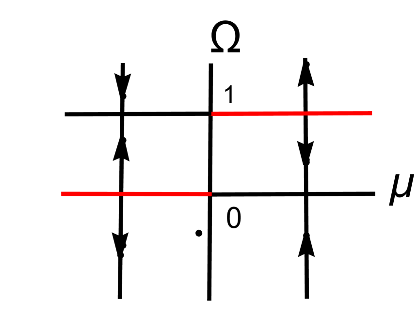
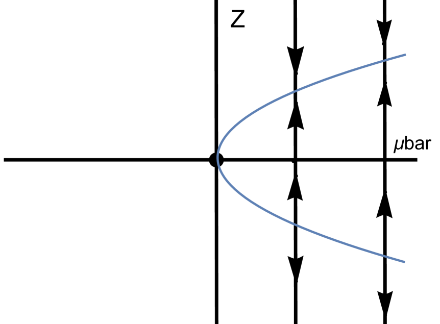
Figure 1: The standard (left) and bifurcation (right) density parameter evolution in Friedmann cosmology compared.

This is the picture one knows from the case of standard Friedmann cosmology.

We then apply the bifurcation sequence steps of Section 4 and arrive at the versal unfolding $Z^{\prime}=\bar{\mu}-Z^{2}$, and the bifurcation diagram in Figure 1 (right) for the versally unfolded density $Z=1/2-\Omega$, where $\bar{\mu}=1/4-\sigma/\mu$, with $\mu\neq 0$, and $\sigma$ is the unfolding parameter which describes physically the closeness of the models to the unperturbed Friedmann universe (this can be made precise).

We note that in this problem both the parameter space and the phase space are one-dimensional, and the bifurcation takes place at the origin of the $(Z,\mu)$-plane.

This leads to physical effects associated with the appearance of the new branch of fixed points, namely, the parabola shown in the Fig. 1 (right). Several features of the standard cosmological picture are now replaced by novel properties stemming from this Figure.

For example, the equilibrium solutions 0 and 1 of the evolution equation for the density parameter $\Omega$ in standard cosmology are now absent and are replaced by new perturbed equilibria, i.e., pairs of the form $\pm\sqrt{\bar{\mu}}$. This has various implications that will be considered elsewhere.

We also note in passing the following important application of the versally unfolded Friedmann evolution. Although the original Friedmann equations cannot lead to domain synchronization in the dynamical sense considered in [19], Sect. 8, the versal unfolding $Z^{\prime}=\bar{\mu}-Z^{2}$ indeed synchronizes the universe asymptotically, either to the future or the past. This in turn leads to a novel approach to the horizon problem, as explained in detail in [19].

Under parameter variation the novel solutions ((un)stable with the (minus) plus sign) appear on the parabola for positive values of the parameter (the vertical lines being the $Z$-phase spaces), coalesce at the origin and disappear for negative values of the parameter.

These novel forms of evolution are collectively described by what is known as a saddle-node bifurcation, the simplest kind of change of forms in bifurcation theory (the phase portraits for the saddle-node are very standard and not shown presently).

The perturbed equilibria possess further novel properties which we only briefly mention here (we direct the reader to [19] for more details and complete proofs):

1. unlike the situation in standard cosmology no singularities exist in this case,

2. the plus-sign equilibrium in each pair describes stable accelerating universes for a negative unfolding parameter (i.e., when $\bar{\mu}>1/4$ in Fig. 1, right), still all energy conditions are nevertheless satisfied (that is for $\gamma>2/3$).

5.2 The Oppenheimer-Snyder black hole

In this subsection we closely follow [20], Sect. 7 and parts of Sect. 8. The standard Oppenheimer-Snyder (‘OS’) result describing the optical disconnection of the exterior spacetime and the formation of a singularity at the centre of the black hole in a finite time follows from their solution $e^{x}=(F\tau+G)^{4/3}$, where $x$ stands here for the OS comoving function $\omega$, $F,G$ are arbitrary functions of the radial coordinate $R$, and one uses the Schwarzschild metric in comoving coordinates.

The Einstein equations for this problem are equivalent to the system $\ddot{x}+(3/4)\dot{x}^{2}=0$, for which the phase portrait orbits show the characteristic OS diverging behaviour (cf. [20]).

It is an instructive initial conclusion borne out of an application of the bifurcation/singularity theory steps described above, that:

• the OS-system is very degenerate and when written in normal form the Jordan form is the nilpotent matrix.

• the normal form in terms of the $x,y$ variables (as defined) includes 3rd -order terms: $\dot{x}=y,\dot{y}=sx^{3}-x^{2}y$, with $s=\pm 1$ is a modular coefficient. We shall call this the Bogdanov-Takens normal form of order-three.

• all second-order terms in the OS-equation can be eliminated.

The versal unfolding for the OS problem thus requires the inclusion of 3rd-order terms for determinacy, and the problem is of codimension two.

We note the planar parameter spaces here rather than the parameter lines we met in the Friedmann problem in Fig. 1, and the two parameters, namely, deviation from spherical symmetry and rotation, make up the bifurcation diagrams for the deformations. These are shown in the two figures 2, 3 below corresponding to positive and negative modular coefficients respectively.

In these diagrams, we imagine a point moving in parameter space on a small circle around the origin and consider the corresponding motion of a phase point moving on some orbit in one of the phase spaces shown. As the parameter point moves around in parameter space, the phase portraits smoothly transfigure and the phase point drags away from one phase diagram to the next and gradually passes through the various metamorphoses of the different topological states (i.e., phase portraits in this case) as shown.

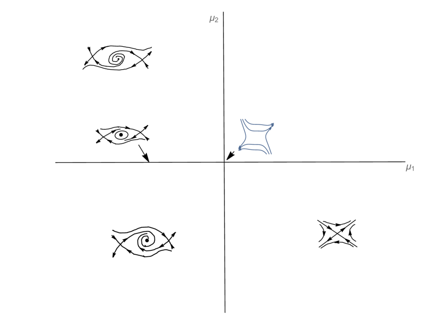
Figure 2: The bifurcation diagram for the Oppenheimer-Snyder-system, positive moduli case.

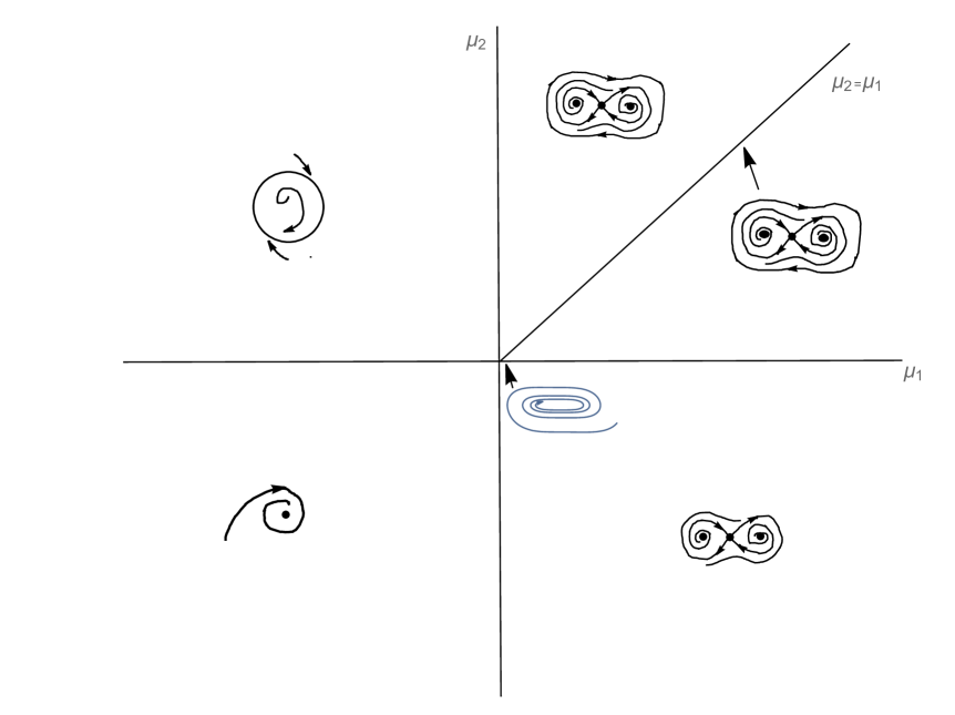
Figure 3: The bifurcation diagram for the Oppenheimer-Snyder-system, negative moduli case.

Three basic features of these diagrams are:

1. the initial formation of trapped surfaces corresponding to the phase point being on one of the escaping orbits in the diagram on the right half of Fig. 2.

2. the formation of stable closed orbits for various values of the parameters in the left part of the diagram.

3. upon parameter variation, the singularities that would have possibly resulted from trapped surface formation and the OS solution seem to be stably bypassed. The system instead smoothly transfigures its phase portraits as shown, and any phase point is able to follow other orbits thus easily avoiding staying too long on any runaway orbit.

This is a very rich situation with novel features unlike anything in the original OS analysis. In addition, we note that there are additional global bifurcations not shown in these figures.

This constitutes a clear prediction of the physics associated with the versal unfolding in this problem. Under parameter variation, a trapped surface may initially form but such a configuration is always unstable and transfigures into something else precisely defined depending on the position of the parameter point in the stratified space (we recall a stratum as a region in parameter space between two consequent bifurcation sets, e.g., between say a bifurcation axis and a bifurcation line, etc).

5.3 Spacetime metamorphoses

In this problem we revisit the evolutionary aspects of the analysis that leads to the singularities in gravitational collapse to a black hole and in a cosmological setting, cf. [20], Sections 5, 6. In terms of the Komar-Landau-Raychaudhuri and the Newman-Penrose-Sachs equations, this analysis constitutes another manifestation of the power of bifurcation theory.

Firstly, it allows for a complete analysis of the nonlinear feedback and coupling effects between the expansion, shear, and vorticity of a geodesic congruence in spacetime taking into full account all degeneracies of this problem. There are two cases, namely, the convergence-shear and the convergence-vorticity systems (subsystems of the Sachs optical equations), and we shall discuss presently the main ideas and results of the first case (this is in fact the only case considered in the classical references).

Secondly, one can now revisit the classical prediction about the existence of a focussing state. In the classical references this question is of course decided based on the analysis of the Raychaudhuri inequality $\rho^{\prime}\geq\rho^{2}$ for the convergence of the spacetime congruence leading to the prediction of spacetime singularities.

Applying the methodology of Sec. 4 to the convergence-shear and the convergence-vorticity dynamical equations leads to codimension-two problems and the final bifurcation diagrams are shown in Figs. 4, 5 respectively. Here the parameters $\mu_{1}$ and $\mu_{2}$ are related to the full projections of the Ricci curvature along a timelike vector and the Weyl curvature along a null tetrad (and rotation parameter respectively for the vorticity case), and the phase space variables are the convergence and the shear (resp. vorticity) of the geodesic congruence.

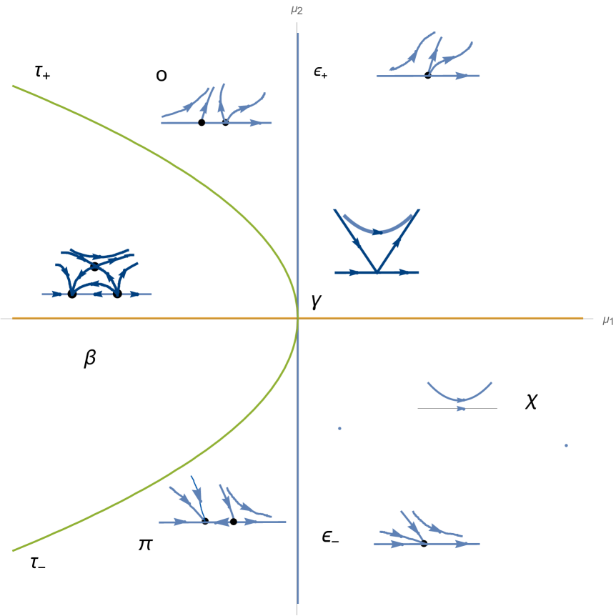
Figure 4: The complete bifurcation diagram for the NPR-system.

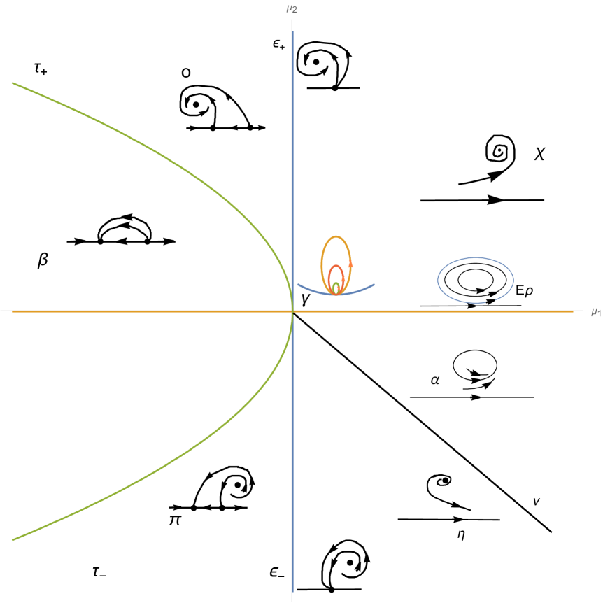
Figure 5: The complete bifurcation diagram for the convergence-vorticity system.

As the parameter point moves on a small circle around the origin in the plane, the phase portraits smoothly transfigure to one another, and a phase point rides around from one phase portrait to the next. For instance, the transition from $\chi$ to $\varepsilon_{-}$ to $\pi$ to $\tau_{-}$ to $\beta$ strata (or for the opposite direction) is accompanied by ‘metamorphoses’ of non-equivalent phase diagrams as shown containing 0 to 1 to 2 to 3 equilibria respectively (or in reverse).

In the emerging physics of the versal unfolding (instead of the standard physical conclusions based on the Raychaudhuri inequality) there are several novel physical effects, and we only note here two, namely, the possibility of spacetime metamorphoses and the ‘ghost effect’ associated with a square root scaling law. Both these effects make the existence of an all-encompassing singular state in general relativity less plausible.

Had the bifurcation diagram in Fig. 4 contained only the $\chi$-stratum (i.e., only the right half-space), there would be one phase portrait and nothing else as is the case with the Raychaudhuri inequality. In that case, there would be of course no possibility for a metamorphosis because the focussing state leading to a singularity would be an inevitable feature of the dynamics (corresponding to the diverging orbits in the $\chi$-phase portrait, the only kind of orbit there).

However, here the situation is rather different: the system exhibits two kinds of bifurcations, namely, a pair of saddle-nodes dominated by the convergence $\rho$, and a pair of pitchfork bifurcations dominated by the shear $\sigma$ (recall that while the saddle-node bifurcation is the basic mechanism by which equilibria are created and destroyed, a pitchfork comes in two types, the supercritical by which an unstable equilibrium slowly decays into two new stable ones, and the subcritical where the system destabilizes).

A saddle-node bifurcation takes the system from the region of attractive gravity $\mu_{1}>0$ where all the energy conditions hold, to the repulsive gravity $\mu_{1}<0$, and back, while a pitchfork occurs in the repulsive gravity region of the parameter space (supercritical for $o\to\tau_{+}\to\beta$, subcritical for $\pi\to\tau_{-}\to\beta$ and back). The evolution of the system is characterized by the combined effects of all these bifurcations.

A second notable feature of the bifurcation dynamics, the ghost or ‘bottleneck’ effect, is related to the saddle-node evolution from and to the $\chi$-stratum, the ‘singularity-forming region’, and implies that the system delays its evolution upon entering the $\chi$-stratum with the delay time scaling as $\mu_{1}^{-1/2}$, a parameter-dependence of the time to the ‘singularity’ as a square-root scaling law, also absent in standard treatments.

5.4 Evolution of event horizons

The problem of studying crease structures defined as endpoints of at least two horizon generators on the event horizon of a generic black hole as 2-dimensional spacelike submanifolds is here reformulated as an evolution problem of the crease submanifolds governed by a new dynamical system, the crease flow [21]. This replaces the usual Hamiltonian flow wherein the crease sets appear as its steady-state (i.e., fixed point) solutions, while their bifurcations describe the possible types and topological transformations of the singularities very accurately.

The crease flow introduced in [21] deals with the dynamics of event horizons at caustic points where the usual Taylor expansions used in the literature break down, and consequently it becomes unclear how to make physical sense and describe the evolution that develops such caustics. This has a number of benefits over previous approaches to the problem.

We may write down the defining equations of a wave front for this problem (obtained from the event horizon by extending the generators beyond their past end points as far as possible) as the union of two null hypersurfaces in spacetime intersecting transversally.

The intersections are given by the equations $u-b_{AB}x^{A}x^{B}=0,\,v-c_{AB}x^{A}x^{B}=0$, where $(u,v)$ are null coordinates, $A,B=1,2$, $x,y$, are normal coordinates (the ‘transverse’ phase space), and we expand in normal coordinates up to second order terms with the $b,c$ being quadratic polynomials in $x,y$.

We can use suitably defined 2-spheres of radius $\lambda=\sqrt{uv-T^{2}}$, $T$ being a time function (synchronous coordinate) in the place of the null coordinates so that to any given point $(u,v)$ there corresponds a value of $\lambda$, and the $\lambda$-lines screen the $(u,v)$-plane. We then introduce the crease flow for the evolution of the crease sets as that governed by the dynamical system,

$$\begin{split}\dot{x}&=\lambda+b_{AB}x^{A}x^{B}:\quad g_{1},\\ \dot{y}&=\lambda+c_{AB}x^{A}x^{B}:\quad g_{2},\end{split}$$ (5.1)

where the dot means differentiation with respect to the time function, and $x=x^{1},y=x^{2}$ as above. The significance of this system is that in the transverse phase space $(x,y)$, a point $(x_{0},y_{0})$ is an equilibrium solution of the crease system if and only if it lies on a crease submanifold.

The correct nondegeneracy and transversality conditions on the crease flow imply that the crease evolution is a bifurcation problem of codimension three. This result requires the deployment of several notions of singularity theory into this problem (for instance the nature of the Jacobian of the crease flow at the origin).

Further, the bifurcation sequence developed in Section 4 can be applied to the crease flow leading to three different normal forms and corresponding versal unfoldings (each of which having one distinguished parameter, the $\lambda$, and three unfolding parameters). These results depend on the nature of the zero set and the sign of the discriminant of the Jacobian, making the present problem perhaps the most complicated among all those analysed so far (with the possible exception of the Friedmann-Lemaître problem - see below).

We may depict the resulting situation in projections where two of the unfolding parameters are set to zero. In this representation, the problem is described by the bifurcation diagram shown in Fig. 5 we met earlier in shifted variables $X,Y$ and parameters $\mu_{1},\mu_{2}$ (one of them is the $\lambda$ and the other one of the unfolding parameters, cf. [21], Eq. (14)).

In the bifurcation diagram of Fig. 5, we see the resulting ‘liquid-like’ picture of evolving, in principle observable, bifurcating caustics on the event horizon corresponding to intersections of null hypersurfaces in spacetime. This is based on the joined effects of the three possible bifurcations in this problem, namely, saddle-node when crossing any of the two axes, pitchfork when crossing the parabola, and Hopf when crossing the positive $\mu_{1}$-axis, acting on the following caustics: swallowtail, folded Whitney, and a pair of ‘embedded in each other’ (i.e., combined) Whitney singularities, all three being steady states of the crease flow. Using $z$ as a third coordinate, the latter are given by the forms  $x^{2}=zy^{2}$ (standard Whitney), and $x^{2}=z^{3}y^{2}$ (folded).

As the parameter changes differently at different spacetime points, these effects occur simultaneously, thus offering a very rich picture for the evolution of the crease sets. We also note the formation of the stable isolated limit cycle in the $\alpha$-stratum attracting nearby orbits and disappearing upon crossing the $\nu$-line into the $\eta$-stratum.

5.5 The Friedmann-Lemaître equations

We shall write the standard Friedmann-Lemaître equations in the following equivalent form as a dynamical system for the Hubble parameter $H$ and the fluid density $\rho$,

$$\dot{H} = -\frac{3\gamma-2}{6}\rho+\frac{\Lambda}{3}-H^{2}$$ (5.2)

$$\dot{\rho} = -3\gamma H\rho,$$ (5.3)

with the algebraic constraint,

$$a^{2}=\frac{3k}{\rho+\Lambda-3H^{2}}$$ (5.4)

where the scale factor $a(t)$ is a function of the proper time $t$, we have a perfect fluid source with density $\rho$ and pressure $p$ with fluid parameter defined by the equation $p=(\gamma-1)\rho$, a cosmological constant $\Lambda$, and we have set $8\pi G=c=1$, while $k=0,\pm 1$ denotes the normalized constant curvature of the spatial 3-slices.

One may show that the roles of the two parameters of the problem $\gamma,\Lambda$ is different: although $\gamma=0$ is a singularity, $\Lambda$ is a true bifurcation parameter with bifurcation point at $\Lambda=0$. In particular, after moving the de Sitter space and Einstein static universe to the origin, split off the linear parts, and set $\Lambda=0$ the Friedmann-Lemaître equations take the form,

$$\left(\begin{array}[]{c}\dot{H}\\ \dot{\rho}\\ \end{array}\right)=-\frac{(3\gamma-2)}{6}\left(\begin{array}[]{cc}0&1\\ 0&0\\ \end{array}\right)\left(\begin{array}[]{c}H\\ \rho\\ \end{array}\right)+\left(\begin{array}[]{c}-H^{2}\\ -3\gamma H\rho\\ \end{array}\right).$$ (5.5)

This is the basic ‘degenerate core’ of the Friedmann-Lemaître equations. It is $(\mathbb{Z}_{2}+t)$-equivariant, meaning that the system is invariant under the symmetry,

$$H\to-H,\quad\rho\to\rho,\quad t\to-t.$$ (5.6)

We shall call the appearance of this symmetry in the final topological normal form a ‘time-symmetric case’, whereas the case without the $t\to-t$ part a ‘time-asymmetric case’.

The presence or absence of the time symmetry together with the set of $\gamma$-values shown in Fig. 6 fully determine the versal dynamics of the Eq. (5.5) and thus of the original Friedmann-Lemaître equations. Following the bifurcation sequence of steps explained in Section 4, we arrive and the normal forms, versal unfoldings and bifurcation diagrams corresponding to the Friedmann-Lemaître dynamical equations.

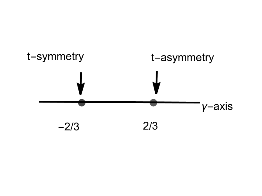
Figure 6: The axis of the parameter $\gamma$. Away from the two shown values of $\gamma$, the system can be either time-symmetric or time-asymmetric. In either case, a passage through the time-(a)symmetric value $-2/3$ (resp. $2/3$) dualizes the behaviour of a time-(a)symmetric that existed for the system when $\gamma\neq\pm 2/3$.

There are four inequivalent cases for the versally unfolded Friedmann-Lemaître system, in total nine bifurcation diagrams. We briefly review this problem in the next four subsections below (for more details the reader is directly to [22]).

5.5.1 The $\gamma=-2/3$ case

The bifurcation diagrams correspond to the so-called cubic Bogdanov-Takens bifurcation, namely,

$$\begin{split}\dot{X}&=Y,\\ \dot{Y}&=\mu_{1}X+\mu_{2}Y\pm X^{3}-X^{2}Y,\end{split}$$ (5.7)

and can be found in figs. 2, 3 for the $(+)$ and the $(-)$ case respectively. The most characteristic metamorphoses here are related to pitchfork and Hopf bifurcations.

5.5.2 The $\gamma=2/3$ case

The bifurcation diagrams correspond to those of the $\mathbb{Z}_{2}$-symmetric versal family [45], namely,

$$\begin{split}\dot{X}&=\mu_{1}+X^{2}+sY^{2},\\ \dot{Y}&=\mu_{2}Y+2XY+X^{2}Y,\end{split}$$ (5.8)

and can be found in Figs. 4, 5 for the $(+)$- and $(-)$-case respectively ($s=\pm 1$).

5.5.3 The FL cusp

Using similar methods as before, one is led to the construction of the bifurcation diagrams in this case too and the resulting versal dynamics. The bifurcation diagrams describe the FL cusp and correspond to the quadratic Bogdanov-Takens versal family [22],

$$\begin{split}\dot{X}&=Y,\\ \dot{Y}&=\mu_{1}+\mu_{2}Y+X^{2}\pm XY,\end{split}$$ (5.9)

and may also be found in, for instance, [6], pp. 444-5, for the $(+)$-case, and [9], p. 358 or [46], p. 1038, Fig. 15 for $(-)$-case.

5.5.4 Codimension-3

The bifurcation diagrams for the codimension-3 FL cubic (cf. [22]), namely,

$$\begin{split}\dot{X}&=Y,\\ \dot{Y}&=\mu_{1}+\mu_{2}X+\mu_{3}Y\pm X^{3}+BXY,\end{split}$$ (5.10)

can be found in [46], figs. 3, 4 for the saddle case, figs. 7, 8 for the focus case, and figs. 13, 14 for the elliptic case (see also [47]).

This is the dynamically richest case among all versally unfolded FL cosmologies (for more details, see [22]).

5.5.5 Some remarks

The relations of the $X,Y$ variables to the original ones for each of the four main case discussed in the previous four subsections is given in [22]. The most important conclusion is related to the global behaviour of the system as $\gamma$ varies, the time-symmetry appears and disappears as $\gamma$ passes through the two values $\mp 2/3$, and the unfolding parameters also change.

Suppose that the system is found itself in one of the five possible ‘ranges’ of $\gamma$-values as in Fig. 6 (the two point values are also regarded as two of these ranges). Then the consequent behaviour of the system is completely determined by the unfolding parameters $\mu_{i},i=1,2$ (and also $\mu_{3}$ for the codimension-3 unfolding (5.10)), in the sense that it moves from one bifurcation diagrams to the next as $\gamma$ varies, and from phase portrait to the next as the unfolding parameters $\mu$ vary, all these transfigurations being smooth.

We note however that the relations of the versal variables $X,Y$ to the parameters $\gamma,\mu$ are not generally smooth and contain a degree of roughness. This is due to the fact that such inversions are not smooth (or even continuous) because of the violation of the implicit function theorem. Thus although the global metamorphoses of the universes versally are all smooth, this is not true for the relations of the solutions to the parameters of the problem.

6 Discussion

This work describes the path from the large body of known and well-understood results related to hyperbolic-like approaches in general relativity to a consistent structurally stable framework, a new but yet largely unknown structure that emerges when unfolding general relativistic systems as the five ones described in this paper. This ‘theory’ eventually contains all versal unfoldings of general relativity.

Our approach to this problem is based on fundamental mathematical works in the subject of bifurcation theory, starting by H. Poincaré around the 1890, developed further by A. A. Andronov, R. Thom, V. I. Arnold, later by F. Takens, R. I. Bogdanov, and more recently by F. Dumortier, H. Zoladek, and many other mathematicians.

In this connection, we make the following remarks. Consider the Einstein equations with a cosmological constant $\Lambda$ considered as a parameter in the sense advanced in this paper. This is clearly an unfolding of the vacuum Einstein equations, but is it a versal unfolding of them? According to the work in this paper, the answer to this question appears to be negative. We have shown that the Einstein equation with $\Lambda$ contains symmetric subsystems, e.g., the FL equations (with $\gamma=0$ in this case), for which the versal unfoldings have codimension greater than one, and three at most. Therefore the Einstein-$\Lambda$ equations have to be versally unfolded and their codimension appears to be at least three. We conjecture that the codimension of the Einstein-$\Lambda$ equations (without matter) is exactly equal to three.

This theory cannot correspond to one with additional action terms, because of the following observation. Consider the FRW problem discussed earlier in Section 5. In that problem, we start from the well-known results about the behaviour of the simplest FRW models and end up with their versal unfolding, namely, the equation $\Omega^{\prime}=\Omega(\Omega-1)+\nu$, where $\nu$ is the unfolding parameter. This is a perturbation of the Friedmann equations via adding lower-order terms (lower with respect to the first nonzero term in the Taylor expansion), and it is versal i.e., all terms of $O(3)$ or higher have no effect on the nature of the bifurcations. As we discussed, the solutions coming from the versal unfolding equation have properties not met in the standard theory and emerge only as bifurcations. In this sense they represent not modifications of the standard theory but a certain completion of it at a deeper level (as we already discussed earlier), one that is very difficult to capture without bifurcation theory. This way gravitational bifurcation theory may considerably expand the present horizon of gravity research.

Obviously one may consider unfolding a theory that contains higher-order curvature terms or is of higher-dimensionality than four, for example in the framework of some modified gravity theory of effective string theory. Although this would lead to interesting projects in gravitational bifurcation theory, we note that there are already some answers to such a problem stemming from the results discussed in this paper. For example, suppose that one considers a Friedmann universe with a perfect fluid with or without a $\Lambda$ in a modified gravity or string theoretic context. If the linear part of the resulting equations turns out to be the same as the corresponding ones discussed here, then the answer will be identical to the ones we found here. This will be so due to the power of the versal unfolding construction. However, the inclusion of other matter fields, for instance a scalar field component, will drastically alter the conclusions and possibly increase the dimensionality of the dynamical systems and/or the codimension of the unfoldings (even in cases with identical symmetries as the ones here, for instance $\mathbb{Z}_{2}$).

Amongst the many fundamental issues emerging in the framework of gravitational bifurcation theory and deserve a comment, we shall briefly discuss only two. Firstly, since the two appear intertwined in any bifurcation diagram, what is the relation between the unfolding parameter (‘motion’ in parameter space) and the time (evolution in phase space)? In particular, which of the two $\mu$ or $t$ is prior? Unconstrained motion in parameter space appears to be a cause for the appearance of a ‘time succession’ in phase space. Consider evolution in a stratum without equilibria, e.g., the negative axis in Fig. 1 right, or the $\chi$-stratum in Fig. 4, and the motion of a parameter point around the origin in parameter space. Passing through a bifurcation set changes the number and nature of equilibria and forces the phase point to move on a new orbit in the ‘next’ phase portrait. Such a smooth transition of the phase point between different phase portraits introduces a time progression into the problem associated with a global change (i.e., the appearance of one or more new equilibria). This state of affairs begs the question as to what causes motion in parameter space? We believe that an answer to this question is related to the proven stability of the versal unfolding. In other words, the system collapses when the stability of the whole construction is disrupted, something which as we have shown cannot really happen in a versal unfolding.

A last problem we would like to briefly discuss is related to the question of the structure and nature of the theory that contains all versal unfoldings starting from a given one. We have begun to answering this question for general relativity, but one could perhaps apply similar ideas to other areas of fundamental theoretical physics. What is the nature of the versal families that describe the unfoldings of the Einstein, Maxwell, Schrödinger, or Dirac equations? A way to begin to answer this question may be by looking at systems that couple gravity to other fields in a specialized context, for instance, in a isotropic universe, or a spherically symmetric star, etc. In this sense, one arrives at a new ‘theory’ that ‘pierces’ through the standard ones at degenerate points (e.g., general relativity at the ‘point’ (5.5)) and contains all such versal final forms of the situation one started with. For example, the landscape construction of string theory may have something to do with the versal unfoldings that the original theory contains and these in turn may lead to a new classification of possible string solutions. Another example of this sort would be to start with say the Einstein-Maxwell equations in some simplified context (say for a simple Bianchi model) and unfold. What would be the nature of the resulting theory? We believe that there is a lot to learn by deploying this program for the versal unfoldings of a given theory and discovering their relations to those of a suitably chosen ‘neighbor’.

References

- [1] R. Thom, Structural Stability and Morphogenesis (CRC Press, 2018, translation of the original 1972 French edition)
- [2] V. I. Arnold, Lectures on bifurcations in versal families, Russ. Math. Surv. 27 (1972) 54
- [3] V. I. Arnold, Geometrical Methods in the Theory of Ordinary Differential Equations (Springer, 1983)
- [4] J. Guckenheimer and P. Holmes, Nonlinear oscillations, dynamical systems, and bifurcations of vector fields (Springer, 1983)
- [5] V. I. Arnold, Dynamical Systems V: Bifurcation Theory and Catastrophe Theory (Springer, 1994)
- [6] S. Wiggins, Introduction to applied nonlinear dynamical systems and chaos, 2nd. Ed. (Springer, 2003)
- [7] L. Perko, Differential equations and dynamical systems, 3rd Ed. (Springer, 2001)
- [8] J. Hal and H. Koçak, Dynamics and Bifurcations (Springer, 1991)
- [9] Yu. A. Kuznetsov, Elements of Applied Bifurcation Theory, Fourth Ed. (Springer, AMS 112, 2023)
- [10] D. K. Arrowsmith and C. M. Place, An Introduction to Dynamical Systems (Cambridge University Press, 1990)
- [11] J. Carr, Applications of Centre Manifold Theory (Springer, 1981).
- [12] J. D. Meiss, Differential Dynamical Systems (SIAM, 2007)
- [13] S. H. Strogatz, Nonlinear Dynamics and Chaos (Perseus Books Publishing, 1994)
- [14] M. Golubitsky, D. G. Schaeffer, Stable Mappings and their Singularities, (Springer, 1979)
- [15] M. Golubitsky, D. G. Schaeffer, Singularities and Groups in Bifurcation Theory, Volume I (Springer, 1984)
- [16] M. Golubitsky, I. Stewart, D. G. Schaeffer, Singularities and Groups in Bifurcation Theory, Volume II (Springer, 1988)
- [17] V. I. Arnold, V. V. Goryunov, O. V. Lyashko, V. A. Vasiliev, Singularity Theory II: Classification and Applications, In: Dynamical Systems VIII, V. I. Arnold (ed.) (Springer, 1993)
- [18] V. I. Arnold, Carastrophe Theory (Springer, 1986)
- [19] S. Cotsakis, Dispersive Friedmann universes and synchronization, Gen. Rel. Grav. 55 (2023) 61; arXiv:2208.07892
- [20] S. Cotsakis, Bifurcation diagrams for spacetime singularities and black holes, Eur. Phys. J. C 84:35 (2024) 1; arXiv:2311.16000
- [21] S. Cotsakis, The crease flow on null hypersufaces, Eur. Phys. J. C 84 (2024) 391; arXiv:2312.08023
- [22] S. Cotsakis, Friedmann-Lemaître universes and their metamorphoses (preprint); arXiv:2411.17286
- [23] M. W. Hirsch and S. Smale, Differential equations, dynamical systems and linear algebra (Academic Press, 1974)
- [24] V. I. Arnold, Ordinary differential equations (MIT Press, 1978)
- [25] D. K. Arrowsmith and C. M. Place, Dynamical Systems (Chapman and Hall, 1992)
- [26] A. A. Andronov, E. A. Leontovich, I. I. Gordon, and A. G. Maier, Qualitative Theory of Second-Order Dynamical Systems (John Wiley and Sons, New York, 1973)
- [27] F. Dumortier, J. Llibre, and J. C. Artés, Qualitative Theory of Planar Differential Systems (Springer, 2006)
- [28] S. W. Weinberg, Gravitation and cosmology (John Wiley, 1972)
- [29] E. W. Kolb and M. S. Turner, The Early Universe (Addison-Wesley, 1990)
- [30] A. Linde, Particle Physics and Inflationary Cosmology (Harwood Academic Publishers, 1990)
- [31] J. A. Peacock, Cosmological Physics (Cambridge University Press, 1999)
- [32] E. Harrison, Cosmology, the Science of the Universe, 2nd. ed. (CUP, 2000)
- [33] V. Mukhanov, Physical Foundationd of Cosmology (CUP, Cambridge, UK, 2012)
- [34] S. W. Weinberg, Cosmology (OUP, Oxford, 2007)
- [35] P. Peter and J-P. Uzan, Primordial Cosmology, (OUP, 2009)
- [36] G. F. R. Ellis, R. Maartens, M. A. H. MacCallum, Relativistic Cosmology (CUP, Cambridge, UK, 2012)
- [37] P.J.E., Peebles, Cosmology’s Century (Princeton University Press, 2020)
- [38] D. Baumann, Cosmology (Cambridge University Press, 2022)
- [39] O. I. Bogoyavlenski, Methods in the qualitative theory of dynamical systems in astrophysics and gas dynamics (Springer, 1985, New York, NY)
- [40] J. Wainwright and G. F. R. Ellis, Dynamical systems in cosmology (CUP, Cambridge, UK, 1997)
- [41] S. Bahamonde, C. G. Boehmer, S. Carloni, E. J. Copeland, W. Fang, N. Tamanini, Dynamical systems applied to cosmology: Dark energy and modified gravity, Physics Reports Vol. 775-777 (2018) 1-122; arXiv:1712.03107 [gr-qc]
- [42] S. Cotsakis and A. P. Yefremov, 100 years of mathematical cosmology: Models, theories, and problems, Phil. Trans. R. Soc. A380 (2022) 20210191 (Part A); ibid., 20210171, (Part B); arXiv:2203.16443
- [43] A. Einstein, The Meaning of Relativity, 5th Ed. (Princeton University Press, 1956), pp. 163-6
- [44] S. Cotsakis, Dynamical synchronization, the horizon problem, and initial conditions for inflation, Lett. HEP 322 (2023) 1; arXiv:2208.07104
- [45] K. Zholondek, On the versality of a family of symmetric vector fields in the plane, Math. USSR Sbornik 48 (1984) 463
- [46] F. Dumortier and C Rousseau, Cubic Liénard equations with linear damping, Nonlinearity 3 (1990) 1015-39.
- [47] F. Dumortier, R Roussarie, J. Sotomayor, and Henryk Zoladek, Bifurcations of planar vectorfields, Nilpotent singularities and abelian integrals, Lecture Notes in Mathematics (Springer-Verlag, 1991).