Two-detector reconstruction of multiphoton states in linear optical networks

Abstract

We propose a method for partial state reconstruction of multiphoton states in multimode ($N$-photon $M$-mode) linear optical networks (LONs) employing only two bucket photon-number-resolving (PNR) detectors. The reconstructed Heisenberg-Weyl-reduced (HW-reduced) density matrix captures quantum coherence and symmetry with respect to HW operators. Employing deterministic quantum computing with one qubit (DQC1) circuits, we reduce the detector requirement from $M$ to $2$, while the requirement on measurement configurations are retained $\mathcal{O}(M^{\max(3,N)})$. To ensure physicality, maximum likelihood estimation (MLE) is incorporated into the DQC1 reconstruction process, with numerical simulations demonstrating the robustness and efficiency of our approach. This method offers a resource-efficient solution for state characterization in large-scale LONs to advance photonic quantum technologies.

I Introduction

Photonic quantum computing (PQC) is a promising platform for universal quantum computation, offering advantages such as long decoherence times, room-temperature operation, and seamless integration with quantum networks. In particular, linear optical implementations of PQC [1, 2] provide a scalable platform for various computational paradigms, including measurement-based one-way quantum computation [3, 4, 5, 6, 7, 8], gate teleportation [9, 10], KLM protocol [11, 12], and boson sampling [13, 14, 15, 16, 17].

In linear optical quantum computing (LOQC), high-quality quantum state preparation, particularly the generation of entangled states, is crucial for enabling high-fidelity quantum processing in LOQC. Various approaches for specific entanglement generation and detection have been theoretically proposed and experimentally validated [18, 19, 20, 20, 21, 22, 23, 24, 25]. In qubit or qudit systems, the quality of quantum state preparation is typically evaluated through quantum state tomography [26, 27, 28]. For the evaluation of the multiphoton ($N$-photon) state preparation in an $M$-mode LON, one can employ the full state tomography with an $M^{\prime}$-mode reconfigurable LON interferometer followed by $M^{\prime}$ PNR detectors, as outlined by Banchi et al. [29]. The measurement setup is shown in Fig. 1 (a). It requires $\mathcal{O}((M+N)^{N})$ LON configurations with $M$ PNR detectors, or one LON configuration with at least approximately $\mathcal{O}(M^{2}/N)$ PNR detectors for $N\ll M$. The latter scheme reduces the number of configurations, which improve the efficiency in time, but demands additional $M^{2}$ modes and PNR detectors, significantly increasing the experimental cost. It shows a tradeoff between the efficiency in measurement time and cost, which establishes minimum experimental requirement for implementing full state tomography of multiphoton quantum states in multimode LON systems. In particular, as LON systems continuously scale up [31], full state tomography for multiphoton states in multimode LONs is often prohibitively expensive in terms of both time and resources, presenting a major challenge for experimental implementations.

To evaluate state preparation with limited experimental resources, we propose a method that avoids full state tomography of the $d_{M,N}\times d_{M,N}$ density matrix, where $d_{M,N}=\binom{N+M-1}{N}$ represents the dimension of an $N$-photon $M$-mode LON system. Instead, our approach reconstructs a reduced $M\times M$ density matrix, derived from the full density matrix, using only two PNR detectors. While this reduced matrix coarsens the full information of the multiphoton state, it retains the state’s symmetry with respect to Heisenberg-Weyl (HW) operators [32, 33, 34, 35]. We refer to this reduced representation as the HW-reduced density matrix of the multiphoton state.

For multiphoton systems, HW-reduced reconstruction with two PNR detectors extends the state tomography techniques developed for qudit systems [36, 37], leveraging the principles of deterministic quantum computing with one qubit (DQC1) [38]. Our method requires $\mathcal{O}(M^{\max(3,N)})$ measurement configurations, and solely two bucket PNR detectors. To ensure the physicality of the reconstructed HW-reduced density matrix, we incorporate maximum likelihood estimation (MLE) [39, 40, 41] into our approach. Numerical simulations shows that this method effectively extracts partial yet meaningful information about the multiphoton state, providing a resource-efficient alternative for state characterization.

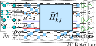
(a)

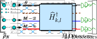
(b)

Figure 1: Evaluation of an $N$-photon $M$-mode quantum state $\widehat{\rho}_{N}$ in linear optical networks (LON). (a) A general schematic for full state tomography of an $N$-photon $M$-mode system in an $M^{\prime}$-mode ($M^{\prime}\geq M$) reconfigurable LON followed by $M^{\prime}$ PNR detectors. The LON interferometer is constructed with tunable Mach-Zehnder interferometers (blue squares). (b) Direct evaluation of a HW operator $\widehat{\Lambda}_{k,l}$ through generalized HW transformation $\widehat{H}_{k,l}$ followed by $M$ PNR detector.

II Reconstruction of HW-reduced density matrix

A single-photon $M$-mode LON system encodes a qudit system with a dimension of $M$, Its quantum state can be fully reconstructed by evaluating the Heisenberg-Weyl (HW) operators $\widehat{\Lambda}_{k,l}:=\widehat{X}^{k}\widehat{Z}^{l}$ [32, 33, 34, 35]. In some conventions, an additional phase factor $\exp(\operatorname{{\mathbbm{i}}}\theta_{k,l})$ is applied to $\widehat{\Lambda}_{k,l}$ to ensure the set of HW operators remains invariant under complex conjugation. However, in the multiphoton regime, such a phase introduces a dependence of $\exp(\operatorname{{\mathbbm{i}}}N\theta_{k,l})$ on the photon number $N$, complicating the state reconstruction. To simplify the process, we omit the phase in our approach.

Here the HW operator is constructed using the mode shift operator $\widehat{X}$ and phase shift operator $\widehat{Z}$. The mode shift operator cyclically shifts a photon to the next neighboring mode, while the phase shift operator applies a phase shift to each output mode. These operations are defined as $\widehat{X}\widehat{a}_{m}^{\dagger}\widehat{X}^{\dagger}=\widehat{a}_{(m+1)\pmod{M}}^{\dagger}$ and $\widehat{Z}\widehat{a}_{m}^{\dagger}\widehat{Z}^{\dagger}=\omega^{m}\widehat{a}_{m}^{\dagger}$, where $\omega:=\exp(\operatorname{{\mathbbm{i}}}2\pi/M)$ is the $M$-th root of the unity. As shown in [36, 37, 43], the expectation values of the HW operators $\widehat{\Lambda}_{k,l}$, can be used to reconstruct the full density matrix of a single-photon $M$-mode state via

$$\rho_{1,M}=\frac{1}{M}\sum_{k,l}\braket{\widehat{\Lambda}_{k,l}}L_{k,l}^{\dagger},$$ (1)

where $L_{k,l}$ is the matrix representation of $\widehat{\Lambda}_{k,l}$ in the single-photon $M$-mode system. Explicitly, the matrix element $L_{k,l}(m,m^{\prime}):=\braket{\cdots 01_{m}0\cdots|\widehat{\Lambda}_{k,l}|\cdots 01_{m^{\prime}}0\cdots}$ is the transition coefficient of mapping the single-photon state from the $m^{\prime}$-th mode to the $m$-th mode.

As shown in Fig. 1 (b), the expectation value of $\widehat{\Lambda}_{k,l}$ in single-photon system can be directly evaluated through the generalized Hadamard transforms, $\widehat{H}_{k,l}$[32, 33, 34, 35], followed by $M$ PNR detections on the output modes. A generalized Hadamard transform $\widehat{H}_{k,l}$, a member of the Clifford group for qudit systems, maps the phase shift operator $\widehat{Z}$ into the HW operator $\widehat{\Lambda}_{k,l}=\widehat{H}_{k,l}\widehat{Z}\widehat{H}_{k,l}^{\dagger}$. Therefore, the expectation value of an HW operator is obtained as $\braket{\widehat{\Lambda}_{k,l}}=\text{Tr}\left(\widehat{Z}(\widehat{H}_{k,l}^{\dagger}\widehat{\rho}\widehat{H}_{k,l})\right)$.

In an $N$-photon $M$-mode LON system, the representation of an HW operator in the full $d_{M,N}$-dimensional Hilbert space spanned by the Fock state basis $\{\ket{\bm{n}}:|\bm{n}|=N,\#\mathrm{mode}(\bm{n})=M\}$ is diagonal with respect to HW-irreducible subspaces [23]. It leads to the fact that the expectation value $\braket{\widehat{\Lambda}_{k,l}}$ of a multiphoton state $\widehat{\rho}$ is invariant under the decoherence with respect to HW subspaces

$$\braket{\widehat{\Lambda}_{k,l}}_{\rho}=\operatorname{{\mathrm{tr}}}\left((\sum_{\mathbb{E}}\widehat{\Pi}_{\mathbb{E}}\widehat{\rho}\widehat{\Pi}_{\mathbb{E}})\widehat{\Lambda}_{k,l}\right),$$ (2)

where $\widehat{\Pi}_{\mathbb{E}}$ is the projection onto the $\mathbb{E}$-spanned HW-irreducible subspaces, and $\mathbb{E}_{\bm{n}}:=\{\widehat{X}^{m}\ket{\bm{n}}\}_{m}$ is generated by the mode shift operator $\widehat{X}$ applied to the Fock state $\ket{\bm{n}}$.

The expectation value of an HW operator is therefore a coarsened information associated with an $M\times M$ density matrix $\rho_{HW}$ reduced from the full $d_{M,N}\times d_{M,N}$ density matrix $\rho$ via a mixture of the density matrix $\rho_{HW}^{(\mathbb{E})}$ within each HW subspace,

$$\rho_{HW}:=\sum_{\mathbb{E}}p_{\mathbb{E}}\,\rho_{HW}^{(\mathbb{E})},$$ (3)

where the entries of $\rho_{HW}^{(\mathbb{E})}$ are obtained from $\rho_{HW}^{(\mathbb{E})}[m,m^{\prime}]=\braket{\widehat{X}^{m}\bm{n}|\widehat{\rho}|\widehat{X}^{m^{\prime}}\bm{n}}d_{\mathbb{E}}/(M\,p_{\mathbb{E}})$, $d_{\mathbb{E}}=|\mathbb{E}|$ is the dimension of the HW-irreducible subspace and $p_{\mathbb{E}}=\operatorname{{\mathrm{tr}}}(\widehat{\Pi}_{\mathbb{E}}\widehat{\rho}\widehat{\Pi}_{\mathbb{E}})$ is the weight of the quantum state in the $\mathbb{E}$-spanned HW subspace (see Definition 4 in Appendix A for the detailed construction of an HW-reduced density matrix.) For a mode number $M$ and a photon number $N$ that fulfill $\gcd(N,M)=1$, the quantum system within each $\mathbb{E}$-spanned HW subspace is a well-defined $M$-dimensional qudit system. The density matrix $\rho_{HW}^{(\mathbb{E})}$ within an HW-irreducible subspace $\mathbb{H}_{\mathbb{E}}$ can be then decomposed as a sum of the HW density matrices $L_{k,l}^{\dagger}$ like the representation of a single-photon state in Eq. (1). As a result, the HW-reduced density matrix of a multiphoton state can be reconstructed via evaluating the HW operators according to the following theorem.

Theorem 1

For an $N$-photon $M$-mode state with $\gcd(N,M)=1$, its HW-reduced density matrix of an $N$-photon $M$-mode quantum state can be reconstructed via

$$\rho_{HW}=\frac{1}{M}\sum_{k,l}^{M-1}\braket{\widehat{\Lambda}_{k,l}}_{\rho}L_{k,Nl}^{\dagger}.$$ (4)

where $L_{k,l}(m,m^{\prime}):=\braket{\cdots 01_{m}0\cdots|\widehat{\Lambda}_{k,l}|\cdots 01_{m^{\prime}}0\cdots}$ is the matrix representation of the HW operator $\widehat{\Lambda}_{k,l}$ in the single-photon subspace.

Proof: This theorem follows as a special case of Theorem 7 in Appendix B.   

Although the HW-reduced density matrix erases the information of quantum coherence among HW subspaces, it retains the symmetry information with respect to HW operators, since the expectation value of each HW operator can be straightforwardly computed as $\braket{\widehat{\Lambda}_{k,l}}=\operatorname{{\mathrm{tr}}}(\rho_{HW}L_{k,l})$ using the HW-reduced density matrix. The measurement configuration of HW-reconstruction via direct HW-operator evaluation is illustrated in Fig. 1 (b). It requires $\mathcal{O}(M^{2})$ measurement configurations and $M$ PNR detectors.

III DQC1 reconstruction using two PNR detectors

The number of required PNR detectors can be significantly reduced employing the deterministic quantum computing with one qubit (DQC1) method. The DQC1 method [38] has been adapted for state reconstruction in qudit systems [36, 37]. In DQC1-based state reconstruction, an auxiliary qubit is introduced to control HW operators on the target qudit system, allowing all HW operators to be efficiently evaluated through qubit measurements of the auxiliary qubit. In a LON system, a qubit can be encoded using dual-rail encoding, which requires only two PNR detectors for qubit measurements. This enables the evaluation of all HW operators with solely two PNR detectors. Extending DQC1 to an $N$-photon $M$-mode LON system allows for the efficient evaluation of all HW operators $\braket{\widehat{\Lambda}_{k,l}}$, which are necessary for HW-reduced density matrix reconstruction as described in Eq. (4), while maintaining the minimal detector requirement.

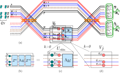
Figure 2: DQC1 measurement. (a) An $M$-mode LON system is extended to $2M$ modes by adding $M$ auxiliary modes via two $M$-mode beam splitters. The $N$-photon testing state $\rho_{N}$ is input to the upper $M$ modes, while the target mode transform $\widehat{U}$ is applied in the lower $M$ modes after the first beam spliter. Combining the two wings by a second beam splitter, at the output, two bucket PNR detectors measure the total photon number $N_{A}$ and $N_{B}$ of the two wings. (b,c) Unitary transformations for evaluating HW operators $\widehat{\Lambda}_{k,l}$ with $k\geq 1$. (d) Phase shifts employed for reconstructing the diagonal elements of $\rho_{N}$.

The DQC1 measurement setup for an $M$-mode LON system is illustrated in Fig. 2 (a). An $N$-photon $M$-mode state $\widehat{\rho}_{N}$ is input into the first $M$ modes of a $2M$-mode LON interferometer, divided into two wings $A$ and $B$. These wings interact through two large beam splitters embedded with a target unitary $\widehat{U}$ in the lower wing. At the output modes, two bucket PNR detectors measure the total photon numbers $N_{A}$ and $N_{B}$ for wings $A$ and $B$, respectively. The Pauli Z-observable $\widehat{\zeta}(U)$ of the qubit space in this $N$-photon $M$-mode DQC1 setup tailored for the unitary $\widehat{U}$ is defined by two projectors, $\widehat{\Pi}_{\pm}$, associated with the parity of the photon number $N_{B}$,

$$\widehat{\zeta}(U)=\widehat{\Pi}_{+}-\widehat{\Pi}_{-}\text{ with }\widehat{\Pi}_{\pm}:=\sum_{(-1)^{N_{B}}=\pm 1}^{N_{A}+N_{B}=N}\widehat{\Pi}_{N_{A}}\otimes\widehat{\Pi}_{N_{B}}$$ (5)

where $\widehat{\Pi}_{N_{A,B}}=\sum_{|\bm{n}_{A,B}|=N_{A,B}}\ket{\bm{n}_{A,B}}\bra{\bm{n}_{A,B}}$ is the projector onto the total photon numbers $N_{A,B}$ on the output wings $A$ and $B$, respectively. The DQC1 Z-observable $\widehat{\zeta}(U)$ is then evaluated from the experimental data by

$$\braket{\widehat{\zeta}(U)}_{\text{DQC1}}=\sum(-1)^{N_{B}}p(N_{B}|N_{A}+N_{B}=N).$$ (6)

One can show that the expectation value of the DQC1 Z-observable evaluates the observable $(\widehat{U}+\widehat{U}^{\dagger})/2$ (Lemma 8 in Appendix C),

$$\braket{\widehat{\zeta}(U)}_{DQC1}=\braket{\frac{1}{2}(\widehat{U}+\widehat{U}^{\dagger})}_{\rho_{N}}=\frac{1}{2^{N}}\braket{\widehat{U}+\widehat{U}^{\dagger}}_{\rho_{N}}.$$ (7)

For single-photon systems $N=1$, which is a well-defined qudit system, the expectation value is linear with respect to the sum of operators, $\braket{\widehat{U}+\widehat{U}^{\dagger}}=\braket{\widehat{U}}+\braket{\widehat{U}^{\dagger}}$. The expectation value of the DQC1 Z-observable is therefore equal to the real part of the expectation value of the target unitary operator $\braket{\widehat{U}}_{\rho}$, expressed as $\braket{\widehat{\zeta}(U)}_{\text{DQC1}}=\mathrm{Re}(\braket{\widehat{U}}_{\rho})$. By configuring the target unitary as $\widehat{U}_{rkl}=(-\operatorname{{\mathbbm{i}}})^{r}\widehat{\Lambda}_{k,l}$, one can extract both the real($r=0$) and imaginary ($r=1$) components of the expectation value of an HW operator $\braket{\widehat{\Lambda}_{k,l}}_{\rho}$ for the single-photon state $\widehat{\rho}_{N=1}$. This enables the full reconstruction of the state $\widehat{\rho}_{N=1}$ employing solely two PNR detectors via Eq. (4).

In multi-photon systems, photon bunching disrupts the linearity of the expectation value, such that $\braket{\widehat{U}+\widehat{U}^{\dagger}}\neq\braket{\widehat{U}}+\braket{\widehat{U}^{\dagger}}$. This nonlinearity prevents the direct evaluation of $\widehat{\Lambda}_{k,l}$ from the DCQ1 Z-observable $\widehat{\zeta}$, thereby complicating the reconstruction of the HW-reduced density matrix in these systems. The nonlinearity arises from photon bunching, which induces transitions between different HW subspaces for the operator $\widehat{\Lambda}_{k,l}+\widehat{\Lambda}_{k,l}^{\dagger}$, while these transitions are not expected for the individual operators $\widehat{\Lambda}_{k,l}$ and $\widehat{\Lambda}_{k,l}^{\dagger}$.

To restore the linearity, we introduce an erasing channel $\mathcal{E}_{k}(\cdot)$ to cancel out the unwanted transitions,

$$\mathcal{E}_{k}(\widehat{U}) =\frac{2^{(1-\delta^{N}_{M})}}{M}\sum_{m}\cos(\frac{2\pi}{M}kmN)\widehat{Z}^{-m}\widehat{U}\widehat{Z}^{m}.$$ (8)

This erasing channel works for $N\geq M/\gcd(2k,M)$ and $k\geq 1$, ensuring that $\braket{\mathcal{E}_{k}(\widehat{\Lambda}_{k,l}+\widehat{\Lambda}_{k,l})}_{\rho}=\braket{\widehat{\Lambda}_{k,l}}_{\rho}+\braket{\widehat{\Lambda}_{k,l}}_{\rho}$ (see Lemma 9 and 10 in Appendix D). The DQC1 evaluation of the erasing channel can be derived from Eq. (7), which leads to the following theorem for DQC1 evaluation of HW operators.

Theorem 2 (DQC1 evaluation of HW operators)

For an $N$-photon $M$-mode state $\widehat{\rho}$, where $N\leq M/\text{gcd}(2k,M)$, the expectation value of an HW operator $\widehat{\Lambda}_{k,l}$ with $k\geq 1$ can be evaluated by

$$\mathrm{Re}\left(e^{\operatorname{{\mathbbm{i}}}\theta N}\braket{\widehat{\Lambda}_{k,l}}_{\rho}\right)$$ (9)

$$= \frac{2^{N-\delta^{2kN}_{0}}}{M}\sum_{m=0}^{M-1}\cos\left(\frac{2\pi}{M}kmN\right)\Braket{\widehat{\zeta}\left(e^{\operatorname{{\mathbbm{i}}}(\theta+\varphi_{km})\widehat{N}}\widehat{\Lambda}_{k,l}\right)}_{\text{DQC1}},$$

where $\delta^{2kN}_{0}=1$ for $2kN\pmod{M}=0$, $\widehat{N}=\sum_{m}\widehat{a}_{m}^{\dagger}\widehat{a}_{m}$ counts the total photon number, and $\varphi_{km}=km(2\pi/M)$.

Proof: see Appendix D.   

Fig. 2 (c) illustrates the DQC1 evaluation of HW operators in a multiphoton LON system. For an HW operator $\widehat{\Lambda}_{k,l}$ with $k\geq 1$, we need to implement the DQC1 measurement with $\widehat{U}_{rklm}=\exp(\operatorname{{\mathbbm{i}}}(\theta_{r}+\varphi_{km})\widehat{N})\widehat{\Lambda}_{k,l}$, where $\varphi_{km}=2\pi km/M$ and $\theta_{r}=-r\pi/(2N)$. One can then obtain the real($r=0$) and imaginary($r=1$) components of $\widehat{\Lambda}_{k,l}$.

For $k=0$, which is associated with the diagonal elements $\rho_{\bm{n}\bm{n}}:=\braket{\bm{n}|\widehat{\rho}|\bm{n}}$ of the density matrix, Theorem 2 does not work. In this case, we choose random phase shifts $\widehat{V}_{j}=\exp(\operatorname{{\mathbbm{i}}}\sum_{m}\varphi_{j,m}\widehat{a}_{m}^{\dagger}\widehat{a}_{m})$ for the DQC1 implementation (see Fig. 2 (d)). The DQC1 evaluation of $\widehat{V}_{j}$ returns

$$v_{j}:=\braket{\widehat{\zeta}(V_{j})}_{DQC1}=\sum_{\bm{n}}\braket{\bm{n}|\frac{1}{2}(\widehat{V}_{j}+\widehat{V}_{j}^{\dagger})|\bm{n}}\rho_{\bm{n}\bm{n}}.$$ (10)

Choosing a set of particular DQC1 configurations $(\widehat{V}_{1},...,\widehat{V}_{d_{M,N}})$, one will obtain a vector of $\bm{v}=(v_{1},...,v_{d_{M,N}})$ from the $d_{M,N}$ DQC1 measurements and establish a linear equation $\bm{v}=C.(\rho_{\bm{n}\bm{n}})_{\bm{n}}$, where $C(j,\bm{n})=\braket{\bm{n}|\frac{1}{2}(\widehat{V}_{j}+\widehat{V}_{j}^{\dagger})|\bm{n}}$. With a proper choice of $\widehat{V}_{j}$ (see Appendix E), one can establish an invertible $C$ matrix and obtain the diagonal element $\rho_{\bm{n}\bm{n}}$ from the inversion of the $C$ matrix, $\rho_{\bm{n}\bm{n}}=\sum_{j}C^{-1}(j,\bm{n})v_{j}$. The diagonal elements of the HW-reduced density can be then obtained with

$$\mathrm{diag}(\rho_{HW})=\left[\sum_{\mu(\bm{n})=0,j}C^{-1}(j,\widehat{X}^{m}\bm{n})v_{j}\right]_{m},$$ (11)

where $m=0,...,M-1$ and $\mu(\bm{n})=\sum_{m}mn_{m}$ is the total mode index of the Fock vector $\bm{n}$ (see Appendix E for details).

For a prime $M$ and $N<M$, one can combine Theorem 1, 2 and Eq. (11) to reconstruct the HW-reduced density matrix from the DQC1 evaluation of $\widehat{\Lambda}_{k,l}$ and $\widehat{V}_{j}$.

Corollary 3

In an $N$-photon $M$-mode LON system with a prime $M$ and $N<M$, one can reconstruct the HW-reduced density matrix of a quantum state using two PNR detectors via

$$\rho_{HW}=\mathrm{diag}(\rho_{HW})+\frac{1}{M}\sum_{k\geq 1,l}^{M-1}\braket{\widehat{\Lambda}_{k,l}}_{\rho}L_{k,Nl}^{\dagger}.$$ (12)

where $\mathrm{diag}(\rho_{HW})$ and $\braket{\widehat{\Lambda}_{k,l}}_{\rho}$ are determined by Eq. (11) and (9), respectively,

The complexity of DQC1 state reconstruction for prime $M$ and $N<M$ requires $\mathcal{O}(M^{3})$ configurations for the off-diagonal elements of $\rho_{HW}$ and $\mathcal{O}((M+N-1)^{N})$ for the diagonal elements. In total, reconstructing the HW-reduced density matrix requires $\mathcal{O}(M^{\max(3,N)})$ configurations, and solely two PNR detectors. However, if only the quantum coherence in the off-diagonal elements is needed, $\mathcal{O}(M^{3})$ configurations suffice.

IV DQC1 reconstruction with maximum likelihood estimation

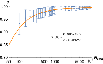
(a)

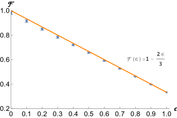
(b)

Figure 3: DQC1 reconstruction using MLE for $2$-photon $3$-mode states. (a) Random pure state samples. The fidelity of DQC1 reconstruction using MLE is plotted as a function of the number of shots $N_{\text{shot}}$ per measurement configuration. For each $N_{\text{shot}}$, $50$ simulation runs were conducted, with a random $2$-photon $3$-mode state selected as the testing state for each run. The blue dots indicate the average fidelity and standard deviation across the $50$ simulations, while the orange line represents a non-linear fit model. (b) Robustness against white noise. The measurement shot number $N=780$ is fixed. The uniform superposition state $\ket{\psi}=(\ket{011}+\ket{101}+\ket{110}+\ket{200}+\ket{020}+\ket{002})/\sqrt{6}$ is mixed with the white noise weighted by $\epsilon$. For each $\epsilon$, $50$ simulations were conducted. The blue dots represent the average fidelity and standard deviation, while the orange line shows the theoretical prediction.

In experiments, limited measurement shot numbers leads to deviations in the evaluation of the Pauli $Z$-operator in DQC1 measurements, resulting in an unphysical HW-reduced state. To address this, maximum likelihood estimation (MLE) [39, 40, 41] can be employed to restore the physicality of the reconstructed state.

Since all measurements in DQC1 reconstruction are qubit-based, the standard MLE method can be used to construct a likelihood function. This function is based on the theoretical expectation values of HW operators $\widehat{\Lambda}_{k,l}$ for $k\geq 1$ and the phase operators $\widehat{V}_{j}$ for $k=0$ derived from Eq. (12). Details for constructing the likelihood function are provided in Appendix F.

The quality of DQC1 reconstruction of an input state $\rho_{HW}^{(in)}$ is evaluated using the state fidelity $F_{N}(\rho_{HW}^{in},\rho_{HW}^{MLE})=\operatorname{{\mathrm{tr}}}(\sqrt{\sqrt{\rho_{HW}^{MLE}}\rho_{HW}^{in}\sqrt{\rho_{HW}^{MLE}}})^{2}$. Increasing the shot numbers per measurement configuration improve the estimation fidelity approaching $1$. A good choice of the set of $\widehat{V}_{j}$ phase shifts, such that the invertible matrix $C$ in Eq. (11) has a large determinant, allows a fast convergence with respect to the shot number (see Appendix F for details).

We simulated DQC1 reconstruction for $2$-photon $3$-mode states. The best choice of $\widehat{V}_{j}$ is numerically determined and given in Fig. 4. To test efficiency, we fix the shot number $N$, randomly select pure states $\ket{\psi_{i}}$, implement the DQC1 reconstruction to reconstruct $\rho_{HW,i}$, and calculate fidelities $F_{N,i}$. We then evaluate the average and deviation of $\{F_{N,i}\}_{i}$ for different shot number $N$. The results, shown in Fig. 3 (a), demonstrate rapid fidelity convergence to $1$, achieving an average fidelity of $0.9$ with just $N_{\text{shot}}=100$ shots. For a target fidelity of $0.99$, only $N_{\text{shot}}=780$ shots are needed, highlighting the robustness and efficiency of our DQC1 state reconstruction.

In another simulation, we test the robustness of our method against white noise using the state $\ket{\psi}=(\ket{011}+\ket{101}+\ket{110}+\ket{200}+\ket{020}+\ket{002})/\sqrt{6}$ and introducing white noise modeled as $\rho_{\epsilon}=(1-\epsilon)\ket{\psi}\bra{\psi}+\epsilon\widehat{\operatorname{\mathbbold{1}}}/d_{M,N}$. The result demonstrates the resilience of our method to the white noise, as the simulated fidelity, shown in Fig. 3 (b), aligns well with the theoretical prediction $F=1-(1-1/M)\epsilon$.

V Conclusion and discussion

We have developed a method for partial state reconstruction of multiphoton states in multimode ($N$-photon $M$-mode) linear optical network (LON) systems using only two bucket photon-number-resolving (PNR) detectors. The reconstructed density matrix, an $M\times M$ Heisenberg-Weyl-reduced (HW-reduced) density matrix defined in Eq. (3), encodes the symmetry properties with respect to HW operators $\widehat{\Lambda}_{k,l}$. The HW-reduced density matrix provides a coarse-grained mixture of $M\times M$ density matrices, which are projected from the multiphoton state onto HW subspaces.

The HW-reduced density matrix can be reconstructed by evaluating HW operators (Theorem 1), originally requiring $M$ PNR detectors and $\mathcal{O}(M^{2})$ measurement configurations. By employing deterministic quantum computing with one qubit (DQC1) circuits, we reduce the detector requirement to just two. Due to nonlinearity introduced by photon bunching, additional $M$ DQC1 measurement configurations are needed for each HW operator $\widehat{\Lambda}_{k,l}$ for $k\geq 1$ (Theorem 2). It allows us to reconstruct the off-diagonal elements of the HW-reduced density matrix and revealing quantum coherence within HW-irreducible subspaces with $\mathcal{O}(M^{3})$ measurement configurations. Meanwhile, for diagonal elements, $\mathcal{O}(M^{N})$ phase shift configurations are required. Ultimately, for a prime $M$ and $N<M$, the HW-reduced density matrix can be fully reconstructed with $\mathcal{O}(M^{\max(3,N)})$ measurement configurations, as shown in Eq. (12) (Corollary 3). Maximum likelihood estimation (MLE) is incorporated into the two-detector DQC1 reconstruction to ensure the physicality of the reconstructed HW-reduced density matrix. Numerical simulations of MLE reconstruction has demonstrated the robustness and efficiency of our method. The two-detector DQC1 reconstruction is applicable to systems with a prime-mode number $M$ and $\gcd(M,N)=1$. An expansion to more general systems is expected in the future.

As LON systems for photonic quantum computing continue to scale up [31], direct characterization becomes increasingly resource-intensive due to the growing number of required detectors. Our method addresses this challenge by providing a two-detector solution for state reconstruction in large-mode systems. Beyond state tomography, this approach is versatile and can be used for tasks such as evaluating multiphoton indistinguishability [44, 45], quantum state fidelity estimation (QSFE) [46, 43], and entanglement detection [22, 24, 23, 25], wherever HW operators need to be evaluated. This makes it a practical and resource-efficient tool for advancing photonic quantum technologies.

Appendix A HW-reduced density matrix and its reconstruction

A HW-reduced density matrix of a multiphoton state is the coarse-grained mixture of density matrices associated with HW-irreducible subspaces. To demonstrate the notion, we employ the $2$-photon $3$-mode LON system as an example. The HW-irreducible subspaces $\mathbb{H}_{110}=\operatorname{span}(\mathbb{E}_{110})$ and $\mathbb{H}_{200}=\operatorname{span}(\mathbb{E}_{200})$ in this LON system are spanned by two sets of Fock states $\mathbb{E}_{110}$ and $\mathbb{E}_{200}$ generated by the mode-shift operator $\widehat{X}$, respectively,

$$\mathbb{E}_{011}:=\{\widehat{X}^{m}\ket{011}\}_{m=0,1,2}\;\;\text{ and }\;\;\mathbb{E}_{200}:=\{\widehat{X}^{m}\ket{200}\}_{m=0,1,2}.$$ (13)

The density matrix of a $2$-photon $3$-mode state is a $6\times 6$ matrix ,

$$\rho=\bNiceMatrix[first-row,first-col,margin=3pt]&\bra{011}\bra{101}\bra{110}\bra{200}\bra{020}\bra{002}\\ \ket{011}\Block[draw=blue,fill=blue!10,rounded-corners]{3-3}{}\rho_{00}\rho_{01}\rho_{02}\rho_{03}\rho_{04}\rho_{05}\\ \ket{101}\rho_{10}\rho_{11}\rho_{12}\rho_{13}\rho_{14}\rho_{15}\\ \ket{011}\rho_{20}\rho_{21}\rho_{22}\rho_{23}\rho_{24}\rho_{25}\\ \ket{200}\rho_{30}\rho_{31}\rho_{32}\Block[draw=red,fill=red!10,rounded-corners]{3-3}{}\rho_{33}\rho_{34}\rho_{35}\\ \ket{020}\rho_{40}\rho_{41}\rho_{42}\rho_{43}\rho_{44}\rho_{45}\\ \ket{002}\rho_{50}\rho_{51}\rho_{52}\rho_{53}\rho_{54}\rho_{55}$$ (14)

The highlighted blue and red blocks represent the density matrices of $\rho$ within the $\mathbb{H}_{011}$ and $\mathbb{H}_{200}$ subspaces, respectively. The Hilbert space $\mathbb{H}_{2,3}$ of $2$-photon and $3$-mode states can be decomposed as a direct sum of $\mathbb{H}_{011}$ and $\mathbb{H}_{200}$, or a tensor product of the qubit space $\mathbb{H}_{\mathbb{E}}$ spanned by $\{\mathbb{E}_{011},\mathbb{E}_{200}\}$ and the qutrit system $\mathbb{H}_{M}$ spanned by $\{\ket{m}\}_{m=0,..,2}$,

$$\mathbb{H}_{2,3}=\mathbb{H}_{011}\oplus\mathbb{H}_{200}=\mathbb{H}_{\mathbb{E}}\otimes\mathbb{H}_{M}.$$ (15)

In the later representation, a Fock state is labeled by its HW subspace and its numbering within the subspace $\ket{\bm{n}}=\ket{n_{\mathbb{E}{,m}}}$. For example, $\ket{011}=\ket{n_{011,0}}$, $\ket{101}=\ket{n_{011,1}}$ and $\ket{101}=\ket{n_{011,2}}$. The HW-reduced density matrix is obtained through the partial trace $\operatorname{{\mathrm{tr}}}_{HW}$ with respect to the HW-subspaces $\mathbb{H}_{\mathbb{E}}$

$$\operatorname{{\mathrm{tr}}}_{HW}(\rho)[m,m^{\prime}]=\sum_{\mathbb{E}}\braket{n_{\mathbb{E},m}|\widehat{\rho}|n_{\mathbb{E},m^{\prime}}}.$$ (16)

Explicitly, the HW-reduced density matrix of the state in Eq. (20) is given by

$$\rho_{HW}=\begin{bmatrix}\rho_{00}+\rho_{33}&\rho_{01}+\rho_{34}&\rho_{02}+\rho_{35}\\[5.0pt] \rho_{10}+\rho_{43}&\rho_{11}+\rho_{44}&\rho_{12}+\rho_{45}\\[5.0pt] \rho_{20}+\rho_{53}&\rho_{12}+\rho_{54}&\rho_{22}+\rho_{55}\end{bmatrix}=p_{011}\rho_{HW}^{(011)}+p_{200}\rho_{HW}^{(200)},$$ (17)

where $p_{\mathbb{E}}=\sum_{m}\braket{n_{\mathbb{E},m}|\widehat{\rho}|n_{\mathbb{E},m}}$ is the weight of the state in $\mathbb{H}_{\mathbb{E}}$, and the density matrix $\rho_{HW}^{(\mathbb{E})}$ within the subspace $\mathbb{E}$ is given by

$$\rho_{HW}^{(\mathbb{E})}[m,m^{\prime}]=\frac{1}{p_{\mathbb{E}}}\braket{n_{\mathbb{E},m}|\widehat{\rho}|n_{\mathbb{E},m^{\prime}}}.$$ (18)

In the $2$-photon $3$-mode LON system, the mode number is prime and $\gcd(M,N)=1$, which ensures that each HW subspace is a well-defined qutrit system. In a general LON system, where the following condition is not fulfilled,

$$M\text{ is prime, and }\gcd(M,N)=1,$$ (19)

the $\mathbb{E}$-subspace density matrix defined in Eq. (18) is not physical any more for some particular HW subspaces $\mathbb{H}_{\mathbb{E}}$, whose dimension $d_{\mathbb{E}}=|\mathbb{E}|$ is a divisor of the mode number $M$. For instance, in a $2$-photon $4$-mode system, the $\mathbb{E}_{0101}$-density matrix will be double counted,

$$\rho_{HW}^{(0101)}=\frac{1}{\rho_{00}+\rho_{11}}\times\bNiceMatrix[first-row,first-col,margin=3pt]&\bra{0101}\bra{1010}\bra{0101}\bra{1010}\\ \ket{0101}\rho_{00}\rho_{01}\rho_{00}\rho_{01}\\ \ket{1010}\rho_{10}\rho_{11}\rho_{10}\rho_{11}\\ \ket{0101}\rho_{00}\rho_{01}\rho_{00}\rho_{01}\\ \ket{1010}\rho_{10}\rho_{11}\rho_{10}\rho_{11}\\ .$$ (20)

To accommodate these situations, we renormalize the $\mathbb{E}$-subspace density matrix with a factor of $d_{\mathbb{E}}/M$.

$$\rho_{HW}^{(\mathbb{E})}[m,m^{\prime}]=\frac{d_{\mathbb{E}}}{Mp_{\mathbb{E}}}\braket{n_{\mathbb{E},m}|\widehat{\rho}|n_{\mathbb{E},m^{\prime}}}.$$ (21)

With this construction, we end up with the definition of the HW-reduced density matrix given in Eq. (3).

Definition 4 (HW-reduced density matrix)

An HW-reduced density matrix $\rho_{HW}$ of a quantum state is a mixture of its $\mathbb{E}$-subspace density matrices,

$$\rho_{HW}=\sum_{\mathbb{E}}p_{\mathbb{E}}\rho_{HW}^{(\mathbb{E})},$$ (22)

where $\rho_{HW}^{(\mathbb{E})}$ is defined as

$$\rho_{HW}^{(\mathbb{E})}=\frac{d_{\mathbb{E}}}{M\,p_{\mathbb{E}}}\braket{\widehat{X}^{m}\widetilde{\bm{n}}|\widehat{\rho}|\widehat{X}^{m^{\prime}}\widetilde{\bm{n}}}\text{ with }\mu(\widetilde{\bm{n}})=0,$$ (23)

where $\mu(\bm{n})=\sum_{m}mn_{m}$ is the total mode index of the Fock vector. Here, $\widetilde{\bm{n}}$ is the representative Fock vector of the HW-irreducible subspace that has $\mu(\bm{n})=0$.

Appendix B Representation of HW-reduced density matrix

In this section, we establish a theorem representing HW-reduced density matrices in terms of HW-operator matrices. To achieve this, we first express HW operators within HW-irreducible subspaces. For this purpose, we adopt a generalized definition of HW operators with specific phases $\theta_{k,l}$,

$$\widehat{\Omega}_{k,l}=\omega^{\theta_{k,l}\widehat{N}}\widehat{\Lambda}_{k,l}=\omega^{\theta_{k,l}\widehat{N}}\widehat{X}^{k}\widehat{Z}^{l},$$ (24)

where $\widehat{N}=\sum_{m=0}^{M-1}\widehat{a}_{m}^{\dagger}\widehat{a}_{m}$. Under the condition of $\gcd(M,N)=1$, each HW subspace is a well-defined $M$-dimensional qudit system. In an HW subspace $\mathbb{E}$, one can always find a Fock vector $\bm{n}$, such that $\mu(\widetilde{\bm{n}})=0$, where $\mu(\bm{n})=\sum_{m}m\,n_{m}$ is the total mode index of the Fock vector. The matrix representation of $\widehat{\Omega}_{k,l}$ within an HW subspace $\mathbb{H}_{\mathbb{E}}$ is then defined as

$$\mathcal{M}_{k,l}^{(\mathbb{E})}[m,m^{\prime}]:=\braket{\widehat{X}^{m}\widetilde{\bm{n}}|\widehat{\Omega}_{k,l}|\widehat{X}^{m^{\prime}}\widetilde{\bm{n}}}\;\;\text{ with }\;\;\mu(\widetilde{\bm{n}})=0.$$ (25)

It turns out that the explicit expressions of $\mathcal{M}_{k,l}^{(\mathbb{E})}$ are identical for the HW-irreducible subspaces $\mathbb{H}_{\mathbb{E}}$ that have the same photon number $N$.

Lemma 5

In an $N$-photon $M$-mode system with $\gcd(N,M)=1$, the matrix representation of an HW operator $\widehat{\Omega}_{k,l}$ within an HW-irreducible subspaces $\mathbb{H}_{\mathbb{E}}$ is given by

$$\mathcal{M}^{(\mathbb{E})}_{k,l}=\omega^{N\theta_{k,l}-\theta_{k,Nl}}\mathcal{M}^{(10\cdots 0)}_{k,Nl}.$$ (26)

Proof: The matrix element of $\Omega_{k,l}$ is determined as

$$\mathcal{M}^{(\mathbb{E})}_{k,l}[m,m^{\prime}]=\omega^{N\theta_{k,l}}\braket{\widehat{X}^{m}\bm{n}|\widehat{\Lambda}_{k,l}|\widehat{X}^{m^{\prime}}\bm{n}}$$ (27)

Since the Fock vector has $\mu(\bm{n})=0$, it holds

$$\braket{\widehat{X}^{m}\bm{n}|\widehat{\Lambda}_{k,l}|\widehat{X}^{m^{\prime}}\bm{n}}=\omega^{Nlm^{\prime}}\braket{\widehat{X}^{m}\bm{n}|\widehat{\Lambda}_{k,0}|\widehat{X}^{m^{\prime}}\bm{n}}=\braket{\widehat{X}^{m}10\cdots 0|\widehat{\Lambda}_{k,Nl}|\widehat{X}^{m^{\prime}}10\cdots 0}.$$ (28)

This results in the following equality

$$\mathcal{M}^{(\mathbb{E})}_{k,l}[m,m^{\prime}]=\omega^{\theta_{k,Nl}-\theta_{k,Nl}}\mathcal{M}^{(10\cdots 0)}_{k,Nl}[m,m^{\prime}]$$ (29)

 

For conciseness, we denote $\mathcal{M}_{k,l}^{(10\cdots 0)}$ by $\mathcal{M}_{k,l}^{(1)}$. In the case $\theta_{k,l}=0$, the HW matrix $\mathcal{M}_{k,l}^{(1)}$ coincides with the HW matrix $L_{k,l}$ in Eq. (1).

As a result of Lemma 5, we arrive at the following lemma for the reconstruction of the density matrix $\rho^{(\mathbb{E})}_{HW}$ within an HW-irreducible subspace.

Lemma 6

For $\gcd(N,M)=1$, The density matrix $\rho^{(\mathbb{E})}_{HW}$ within an HW-irreducible subspace $\mathbb{H}_{\mathbb{E}}$ can be reconstructed by

$$\rho^{(\mathbb{E})}_{HW}=\frac{1}{Mp_{\mathbb{E}}}\sum_{k,l}\operatorname{{\mathrm{tr}}}\left(\widehat{\Omega}_{k,l}(\widehat{\Pi}_{\mathbb{E}}\widehat{\rho}\widehat{\Pi}_{\mathbb{E}})\right)\left(\omega^{N\theta_{k,l}-\theta_{k,Nl}}\mathcal{M}_{k,Nl}^{(1)}\right)^{\dagger}.$$ (30)

where $p_{\mathbb{E}}=\operatorname{{\mathrm{tr}}}(\widehat{\Pi}_{\mathbb{E}}\widehat{\rho}\widehat{\Pi}_{\mathbb{E}})$ is the probability of measuring Fock states in $\mathbb{H}_{\mathbb{E}}$.

Proof: According to Definition 4, the density matrix of $\widehat{\rho}$ in $\mathbb{E}$ is

$$\rho_{HW}^{(\mathbb{E})}[m,m^{\prime}]=\frac{1}{p_{\mathbb{E}}}\braket{\widehat{X}^{m}\widetilde{\bm{n}}|\widehat{\rho}|\widehat{X}^{m^{\prime}}\widetilde{\bm{n}}}\text{ with }\mu(\widetilde{\bm{n}})=0.$$ (31)

For $\gcd(M,N)=1$, the HW subspace $\mathbb{H}_{\mathbb{E}}$ is a well-defined $M$-dimensional qudit system. The density matrix can be therefore decomposed as a sum of the HW matrices $\mathcal{M}_{k,l}^{(\mathbb{E})}$,

$$\rho_{HW}^{(\mathbb{E})}=\frac{1}{M}\sum_{k,l}\operatorname{{\mathrm{tr}}}\left(\mathcal{M}_{k,l}^{(\mathbb{E})}\rho^{(\mathbb{E})}_{HW}\right)\mathcal{M}_{k,l}^{(\mathbb{E})\dagger}.$$ (32)

On the other hand, the expectation value of $\widehat{\Omega}_{k,l}$ in the HW subspace is

$$\frac{1}{p_{\mathbb{E}}}\operatorname{{\mathrm{tr}}}\left(\widehat{\Omega}_{k,l}(\widehat{\Pi}_{\mathbb{E}}\widehat{\rho}\widehat{\Pi}_{\mathbb{E}})\right)=\sum_{m,m^{\prime}}\braket{\widehat{X}^{m}\widetilde{\bm{n}}|\widehat{\Omega}_{k,l}|\widehat{X}^{m^{\prime}}\widetilde{\bm{n}}}\braket{\widehat{X}^{m^{\prime}}\widetilde{\bm{n}}|\widehat{\rho}|\widehat{X}^{m}\widetilde{\bm{n}}}/p_{\mathbb{E}}=\operatorname{{\mathrm{tr}}}(\mathcal{M}_{k,l}^{(\mathbb{E})}\rho_{HW}^{(\mathbb{E})})$$ (33)

Following Eq. (32) and (33), we arrive at

$$\rho_{HW}^{(\mathbb{E})}=\frac{1}{Mp_{\mathbb{E}}}\sum_{k,l}\operatorname{{\mathrm{tr}}}\left(\widehat{\Omega}_{k,l}(\widehat{\Pi}_{\mathbb{E}}\widehat{\rho}\widehat{\Pi}_{\mathbb{E}})\right)\mathcal{M}_{k,l}^{(\mathbb{E})\dagger}.$$ (34)

As a result of Lemma 5, we complete the proof

$$\rho^{(\mathbb{E})}_{HW}=\frac{1}{Mp_{\mathbb{E}}}\sum_{k,l}\operatorname{{\mathrm{tr}}}\left(\widehat{\Omega}_{k,l}(\widehat{\Pi}_{\mathbb{E}}\widehat{\rho}\widehat{\Pi}_{\mathbb{E}})\right)\left(\omega^{N\theta_{k,l}-\theta_{k,Nl}}\mathcal{M}_{k,Nl}^{(1)}\right)^{\dagger}.$$ (35)

 

With Lemma 5 and 6, we are now ready to derive the theorem for the reconstruction of HW-reduced density matrices.

Theorem 7 (Reconstruction of HW-reduced density matrices)

For $\gcd(M,N)=1$, the HW-reduced density matrix of an $N$-photon $M$-mode quantum state $\widehat{\rho}$ can be reconstructed with the expectation values of HW operators $\widehat{\Omega}_{i,j}$ and the HW operator matrix in the single-photon subspace $\mathcal{M}_{k,l}^{(1)}$ via

$$\rho_{HW}=\frac{1}{M}\sum_{k,l}\braket{\widehat{\Omega}_{k,l}}_{\rho}\left(\omega^{N\theta_{k,l}-\theta_{k,Nl}}\mathcal{M}_{k,Nl}^{(1)}\right)^{\dagger}.$$ (36)

Proof: According to Definition 4, the HW-reduced density matrix of $\widehat{\rho}$ in an $N$-photon subspace is given as a mixture of density matrices in different subspaces

$$\rho_{HW}=\sum_{\mathbb{E}_{\bm{n}}:\mu(\bm{n})=0,|\bm{n}|=N}p_{\mathbb{E}_{\bm{n}}}\rho^{(\mathbb{E}_{\bm{n}})}_{HW},\;\;\text{ where }\rho^{(\mathbb{E}_{\bm{n}})}_{HW}[m,m^{\prime}]=\braket{\widehat{X}^{m}\bm{n}|\widehat{\rho}|\widehat{X}^{m^{\prime}}\bm{n}}.$$ (37)

According to Lemma 6, we arrive at the result

$$\rho_{HW}=\frac{1}{M}\sum_{k,l}\operatorname{{\mathrm{tr}}}\left(\widehat{\Omega}_{k,l}(\sum_{\mathbb{E}}\widehat{\Pi}_{\mathbb{E}}\widehat{\rho}\widehat{\Pi}_{\mathbb{E}})\right)\left(\omega^{N\theta_{k,l}-\theta_{k,Nl}}\mathcal{M}_{k,Nl}^{(1)}\right)^{\dagger}=\frac{1}{M}\sum_{k,l}\braket{\widehat{\Omega}_{k,l}}_{\rho}\left(\omega^{N\theta_{k,l}-\theta_{k,Nl}}\mathcal{M}_{k,Nl}^{(1)}\right)^{\dagger}.$$ (38)

 

Appendix C The DQC1 Z observable

The DQC1 configuration, shown in Fig. 2, extends an $M$-mode LON system to $2M$-mode using two multimode beam splitters. This setup projects the $N$-photon system into the qubit space via two bucket PNR detectors, which measure the total photon numbers $N_{A}$ and $N_{B}$ on the upper and lower arms, respectively. The Z observable $\widehat{\zeta}$ in the qubit system, as defined in Eq. (5), is defined by two projectors on the output modes.

$$\widehat{\zeta}=\widehat{\Pi}_{+}-\widehat{\Pi}_{-},\;\;\text{ where }\widehat{\Pi}_{\pm}:=\sum_{(-1)^{|\bm{n}_{B}|}=\pm 1}^{|\bm{n}_{A}|+|\bm{n}_{B}|=N}\ket{\bm{n}_{A}}\bra{\bm{n}_{A}}\otimes\ket{\bm{n}_{B}}\bra{\bm{n}_{B}}.$$ (39)

It corresponds a phase shift operator that add a phase $-1$ on each output mode of lower arm $B$, while add no phase to the upper arm $A$,

$$\widehat{\zeta}\widehat{a}_{m}^{\dagger}\widehat{\zeta}^{\dagger}=\widehat{a}_{m}^{\dagger},\;\;\;\;\text{ and }\;\;\;\;\widehat{\zeta}\widehat{b}_{m}^{\dagger}\widehat{\zeta}^{\dagger}=-\widehat{b}_{m}^{\dagger}$$ (40)

where $\widehat{a}_{m}^{\dagger}$ and $\widehat{b}_{m}^{\dagger}$ are the creation operators of the $m$-th mode on the wing $A$ and $B$, respectively. We can employ the direct sum of the phase operator on $A$ and $B$ to denote $\widehat{\zeta}$,

$$\widehat{\zeta}=(\widehat{\operatorname{\mathbbold{1}}})_{A}\oplus(-\widehat{\operatorname{\mathbbold{1}}})_{B}=\begin{bmatrix}\widehat{\operatorname{\mathbbold{1}}}&0\\ 0&-\widehat{\operatorname{\mathbbold{1}}}\end{bmatrix}$$ (41)

The Z observable for an input state is given by

$$\widehat{\zeta}(U)=\widehat{T}_{\text{DQC1}}(U)^{\dagger}\;\widehat{\zeta}\;\widehat{T}_{\text{DQC1}}(U)$$ (42)

where $\widehat{T}_{\text{DQC1}}(U)=\widehat{H}^{\dagger}(\widehat{\operatorname{\mathbbold{1}}}\oplus\widehat{U})\widehat{H}$ is the mode transformation implemented by the LON interferometer shown in Fig. 2, and $\widehat{H}$ corresponds to the multimode beam splitters, which is a Hadamard gate on the qubit space

$$\widehat{T}_{\text{DQC1}}(U)=\widehat{H}^{\dagger}(\widehat{\operatorname{\mathbbold{1}}}\oplus\widehat{U})\widehat{H}=\frac{1}{2}\begin{bmatrix}\widehat{\operatorname{\mathbbold{1}}}&\widehat{\operatorname{\mathbbold{1}}}\\ \widehat{\operatorname{\mathbbold{1}}}&-\widehat{\operatorname{\mathbbold{1}}}\end{bmatrix}\begin{bmatrix}\widehat{\operatorname{\mathbbold{1}}}&0\\ 0&\widehat{U}\end{bmatrix}\begin{bmatrix}\widehat{\operatorname{\mathbbold{1}}}&\widehat{\operatorname{\mathbbold{1}}}\\ \widehat{\operatorname{\mathbbold{1}}}&-\widehat{\operatorname{\mathbbold{1}}}\end{bmatrix}.$$ (43)

Lemma 8

In an $\widehat{U}$-configured DQC1 transformation $T_{\mathrm{DQC1}}(U)$, the expectation value of the $\widehat{\zeta}$ observable in the $2M$ output modes is equal to the expectation value of $\frac{1}{2}(\widehat{U}+\widehat{U}^{\dagger})$ in the $N$-photon $M$-mode testing system:

$$\braket{\widehat{\zeta}(U)}_{\mathrm{DQC1}}=\Braket{\frac{1}{2}(\widehat{U}+\widehat{U}^{\dagger})}_{\rho}=\frac{1}{2^{N}}\Braket{\widehat{U}+\widehat{U}^{\dagger}}_{\rho}$$ (44)

Proof: An input state $\widehat{\rho}$ in the first $M$ modes is described as $\widehat{\rho}\oplus\ket{0}\bra{0}$ in the extended $2M$-mode system. The DQC1 Z observable for the state $\widehat{\rho}\oplus\ket{0}\bra{0}$ is

$$\widehat{\zeta}(U) =\widehat{B}^{\dagger}(\widehat{\operatorname{\mathbbold{1}}}\oplus\widehat{U}^{\dagger})\widehat{B}\widehat{\zeta}\widehat{B}^{\dagger}(\widehat{\operatorname{\mathbbold{1}}}\oplus\widehat{U})\widehat{B}=\widehat{B}^{\dagger}(\widehat{\operatorname{\mathbbold{1}}}\oplus\widehat{U}^{\dagger})\widehat{X}(\widehat{\operatorname{\mathbbold{1}}}\oplus\widehat{U})\widehat{B}$$

$$=\frac{1}{2}\begin{bmatrix}\widehat{\operatorname{\mathbbold{1}}}&\widehat{\operatorname{\mathbbold{1}}}\\ \widehat{\operatorname{\mathbbold{1}}}&-\widehat{\operatorname{\mathbbold{1}}}\end{bmatrix}\begin{bmatrix}\widehat{\operatorname{\mathbbold{1}}}&0\\ 0&\widehat{U}^{\dagger}\end{bmatrix}\begin{bmatrix}0&\widehat{\operatorname{\mathbbold{1}}}\\ \widehat{\operatorname{\mathbbold{1}}}&0\end{bmatrix}\begin{bmatrix}0&\widehat{U}\\ \widehat{\operatorname{\mathbbold{1}}}&0\end{bmatrix}\begin{bmatrix}\widehat{\operatorname{\mathbbold{1}}}&\widehat{\operatorname{\mathbbold{1}}}\\ \widehat{\operatorname{\mathbbold{1}}}&-\widehat{\operatorname{\mathbbold{1}}}\end{bmatrix}=\frac{1}{2}\begin{bmatrix}\widehat{U}+\widehat{U}^{\dagger}&-\widehat{U}+\widehat{U}^{\dagger}\\ \widehat{U}-\widehat{U}^{\dagger}&-\widehat{U}-\widehat{U}^{\dagger}\end{bmatrix}$$ (45)

The expectation value of $\widehat{\zeta}_{\mathrm{DQC1}}(U)$ for an $N$-photon state $\widehat{\rho}\oplus\ket{0}\bra{0}$ is

$$\braket{\widehat{\zeta}(U)}_{\mathrm{DQC1}}=\operatorname{{\mathrm{tr}}}\left((\rho\oplus\ket{0}\bra{0})\;\widehat{\zeta}(U)\right),$$ (46)

It holds then

$$\braket{\widehat{\zeta}(U)}_{\mathrm{DQC1}}=\operatorname{{\mathrm{tr}}}\left(\widehat{\rho}\frac{\widehat{U}+\widehat{U}^{\dagger}}{2}\right)=\Braket{\frac{1}{2}(\widehat{U}+\widehat{U}^{\dagger})}_{\rho}=\frac{1}{2^{N}}\braket{\widehat{U}+\widehat{U}^{\dagger}}_{\rho}$$ (47)

 

Appendix D DQC1 evaluation of HW operators in multiphoton systems (Proof of Theorem 2)

In multiphoton systems, the linearity of expectation values is not preserved, i.e. $\braket{U+U^{\dagger}}\neq\braket{U}+\braket{U^{\dagger}}$. An example is the 3-mode $\widehat{Z}$ operator, whose mode transformation matrix is $Z_{3}=\text{diag}(1,\omega,\omega^{2})$, with the $3$rd-root of unity $\omega=e^{2\pi i/3}$. For the $2$-photon state $\ket{020}$, we have $\braket{\widehat{Z}_{3}}+\braket{\widehat{Z}_{3}^{\dagger}}=-1$. On the other hand, the mode transformation matrix for $\widehat{Z}+\widehat{Z}^{\dagger}$ is $Z_{3}+Z_{3}^{\dagger}=\text{diag}(2,-1,-1)$, which leads to $\braket{020|\widehat{Z}_{3}+\widehat{Z}_{3}^{\dagger}|020}=1\neq\braket{\widehat{Z}_{3}}+\braket{\widehat{Z}_{3}^{\dagger}}$.

Such a nonlinearity prevents us from evaluating the real part of a unitary $\braket{\widehat{U}}$ through the DQC1 measurement. The nonlinearity of the observable $\widehat{\Lambda}_{k,l}+\widehat{\Lambda}_{k,l}^{\dagger}$ for $k\geq 1$ raises from the non-zero off-diagonal elements with respect to HW subspaces, as no transition between two HW subspaces is expected for a single HW operator $\widehat{\Lambda}_{k,l}$ which is diagonal with respect to HW subspaces. Once we can remove the off-diagonal elements of $\widehat{\Lambda}_{k,l}+\widehat{\Lambda}_{k,l}^{\dagger}$ with respect to HW subspaces, we can restore the linearity and evaluate the real part of $\braket{\widehat{\Lambda}_{k,l}}$ through $2\mathrm{Re}\braket{\widehat{\Lambda}_{k,l}}=\braket{\widehat{\Lambda}_{k,l}}+\braket{\widehat{\Lambda}_{k,l}^{\dagger}}=\braket{\widehat{\Lambda}_{k,l}+\widehat{\Lambda}_{k,l}^{\dagger}}$.

To this end, we introduce an erasing channel $\mathcal{E}_{k}(\cdot)$ in Eq. (8) that eliminates the unwanted nonlinear entries. Explicitly, the total erasing channel $\mathcal{E}$ is constructed from the following erasing channels

$$\mathcal{E}_{k}(U):=\mathcal{E}_{k}^{+}(U)+\mathcal{E}_{k}^{-}(U)\;\;\text{ with }\;\;\mathcal{E}_{k}^{\pm}(U):=\frac{1}{M}\sum_{m}\omega^{\pm mk\widehat{N}}\widehat{Z}^{-m}\widehat{U}\widehat{Z}^{m}$$ (48)

The channel $\mathcal{E}_{k}^{\pm}(U)$ eliminates the matrix entries $\braket{\bm{\nu}|\widehat{U}|\bm{n}}$ for $\mu(\bm{n})-\mu(\bm{\nu})\neq\mp kN$, where $\mu(\bm{n})$ is the total mode index of the Fock vector $\bm{n}$ defined as follows.

$$\mu(\bm{n}):=(\sum_{m}mn_{m})\pmod{M}.$$ (49)

Lemma 9 (Erasing channel in multiphoton LON)

In an $N$-photon $M$-mode LON system, the matrix entries of a linear operator $\widehat{U}$ after the erasing channel $\mathcal{E}_{k}^{\pm}(\cdot)$ are determined as follows,

$$\frac{1}{M}\sum_{m=0}^{M-1}\braket{\bm{\nu}|\mathcal{E}_{k}^{\pm}(U)|\bm{n}}=\delta_{\mu(\bm{n}-\bm{\nu})}^{\mp kN}\braket{\bm{\nu}|\widehat{U}|\bm{n}}.$$ (50)

Proof: For an equal photon number $|\bm{n}|=|\bm{\nu}|=N$, it is obvious that

$$LHS=\frac{1}{M}\sum_{m=0}^{M-1}\omega^{m(\pm kN+\mu(\bm{n}-\bm{\nu}))}\braket{\bm{\nu}|\widehat{U}|\bm{n}}=\delta^{\mp kN}_{\mu(\bm{n}-\bm{\nu})}\braket{\bm{\nu}|\widehat{U}|\bm{n}}.$$ (51)

 

These channels can help us to remove the nonlinear entries in $\braket{\bm{\nu}|\widehat{\Lambda}_{k,l}+\widehat{\Lambda}_{k,l}^{\dagger}|\bm{n}}$, which are identified in the following lemma.

Lemma 10 (Removal of nonlinear entries)

In an $N$-photon $M$-mode LON system, where $N\leq M/\gcd(2k,M)$, the nonlinear entries in $\braket{\bm{\nu}|\widehat{\Lambda}_{k,l}+\widehat{\Lambda}_{k,l}^{\dagger}|\bm{n}}$ are the entries that $\mu(\bm{n}-\bm{\nu})\neq\pm kN$. By removing these entries, one restores the linearity of expectation values,

$$2^{-\delta^{0}_{2kN}}\left(\delta^{-kN}_{\mu(\bm{n}-\bm{\nu})}+\delta^{kN}_{\mu(\bm{n}-\bm{\nu})}\right)\braket{\bm{\nu}|\widehat{\Lambda}_{k,l}+\widehat{\Lambda}_{k,l}^{\dagger}|\bm{n}}=\braket{\bm{\nu}|\widehat{\Lambda}_{k,l}|\bm{n}}+\braket{\bm{\nu}|\widehat{\Lambda}_{k,l}^{\dagger}|\bm{n}}$$ (52)

Here, the delta function is defined under $M$-modulus calculation.

Proof: We first prove the following equality

$$\delta^{-kN}_{\mu(\bm{n-\bm{\nu}})}\braket{\bm{\nu}|\widehat{\Lambda}_{k,l}+\widehat{\Lambda}_{k,l}^{\dagger}|\bm{n}}=\omega^{\mu(\bm{n})l}\delta^{\widehat{X}^{k}\bm{n}}_{\bm{\nu}}.$$ (53)

The LHS is equal to

$$\delta^{-kN}_{\mu(\bm{n-\bm{\nu}})}\braket{\bm{\nu}|\widehat{\Lambda}_{k,l}+\widehat{\Lambda}_{k,l}^{\dagger}|\bm{n}} =\delta^{-kN}_{\mu(\bm{n-\bm{\nu}})}\Braket{\bm{\nu}|(\widehat{\Lambda}_{k,l}+\widehat{\Lambda}_{k,l}^{\dagger})\widehat{X}^{-k}\widehat{X}^{k}|\bm{n}}$$

$$=\delta^{-kN}_{\mu(\bm{n-\bm{\nu}})}\omega^{\mu(\bm{n})l}\Braket{\bm{\nu}|(\widehat{\operatorname{\mathbbold{1}}}+\omega^{lk\widehat{N}}\widehat{\Lambda}_{2k,2l}^{\dagger})|\widehat{X}^{k}\bm{n}}.$$ (54)

Let $\widehat{L}_{k,l}:=\widehat{\operatorname{\mathbbold{1}}}+\omega^{lk\widehat{N}}\widehat{\Lambda}_{2k,2l}^{\dagger}$. The matrix element of $\widehat{L}$ is determined through the following expression

$$\braket{\bm{\nu}|\widehat{L}|\bm{n}}=\frac{1}{\sqrt{\bm{\nu}!\bm{n}!}}\mathrm{Perm}(L[\bm{\nu},\bm{n}]),$$ (55)

where $\mathrm{Perm}(L[\bm{\nu},\bm{n}])$ is the permanent of the $N\times N$ matrix $L[\bm{\nu},\bm{n}]$ induced from its mode transformation matrix $L_{m^{\prime},m}$

$$L[\bm{\nu},\bm{n}]=\{L_{m^{\prime},m}E_{\nu_{m^{\prime}},n_{m}}\}_{m^{\prime},m},\;\;\text{ with }\;\;L_{m^{\prime},m}=\delta_{m^{\prime}}^{m}+\omega^{lk-2lm^{\prime}}\delta_{m^{\prime}+2k}^{m}$$ (56)

where $E_{\nu_{m^{\prime}},n_{m}}$ is a $\nu_{m^{\prime}}\times n_{m}$ matrix with a constant entry $1$,

$$E_{\nu_{m^{\prime}},n_{m}}=\left(\begin{array}[]{ccc}1&\cdots&1\\ \vdots&\ddots&\vdots\\ 1&\cdots&1\\ \end{array}\right)_{\nu_{m^{\prime}}\times n_{m}}.$$ (57)

With two phase shifts $\widehat{Z}^{-j}$ and $\widehat{Z}^{j}$ acting before and after the operator $\widehat{L}$, we define the compound operator $\widehat{J}_{j}:=\widehat{Z}^{-j}\widehat{L}\widehat{Z}^{j}$. Then,

$$\delta^{-kN}_{\mu(\bm{n}-\bm{\nu})}\braket{\bm{\nu}|\widehat{J}_{j}|\widehat{X}^{k}\bm{n}}=\delta^{-kN}_{\mu(\bm{n}-\bm{\nu})}\braket{\bm{\nu}|\widehat{Z}^{-j}\widehat{L}\widehat{Z}^{j}|\widehat{X}^{k}\bm{n}}=\delta^{-kN}_{\mu(\bm{n}-\bm{\nu})}\braket{\bm{\nu}|\widehat{L}|\widehat{X}^{k}\bm{n}}$$ (58)

It holds

$$\frac{1}{M}\sum_{j=0}^{M-1}\delta^{-kN}_{\mu(\bm{n}-\bm{\nu})}\braket{\bm{\nu}|\widehat{J}_{j}|\widehat{X}^{k}\bm{n}}=\delta^{-kN}_{\mu(\bm{n}-\bm{\nu})}\braket{\bm{\nu}|\widehat{L}|\widehat{X}^{k}\bm{n}}$$ (59)

One the other hand,

$$\widehat{J}_{j}=\widehat{\operatorname{\mathbbold{1}}}+\omega^{(l+2j)k\widehat{N}}\widehat{\Lambda}_{2k,2l}^{\dagger}$$ (60)

The transition matrix of $\widehat{J}_{j}$ is

$$\braket{\bm{\nu}|\widehat{J}_{j}|\bm{n}}=\frac{1}{\sqrt{\bm{\nu}!\bm{n}!}}\mathrm{Perm}(J[\bm{\nu},\bm{n}]),$$ (61)

where

$$J_{j}[\bm{\nu},\bm{n}]=\{J_{m^{\prime},m}E[\nu_{m^{\prime}},n_{m}]\}_{m^{\prime},m},\;\;\text{ with }\;\;J_{j;m^{\prime},m}=\delta_{m^{\prime}}^{m}+\omega^{lk+2jk-2lm^{\prime}}\delta_{m^{\prime}+2k}^{m}$$ (62)

In general, the permanent $\mathrm{Perm}(J[\bm{\nu},\bm{n}])$ of the matrix $J[\bm{\nu},\bm{n}]$ is given by

$$\mathrm{Perm}(J_{j}[\bm{\nu},\bm{n}])=\sum_{\sigma}\prod_{\alpha=1}^{N}J_{j;m_{\nu}(\sigma_{\alpha}),m_{n}(\alpha)},$$ (63)

where $m_{\nu}(\alpha)$ and $m_{n}(\alpha)$ are the mode index of the $\alpha$-th photon in the Fock state $\bm{\bm{\nu}}$ and $\bm{\bm{n}}$, respectively. Here, we decompose the set of permutation $\sigma$ according to the cardinality $\kappa_{\bm{\nu},\bm{n}}(\sigma)$ of the mode indices that are changed,

$$\kappa_{\bm{\nu},\bm{n}}(\sigma):=\left|\{\alpha\in\{1,...,N\}:m_{\nu}(\sigma_{\alpha})\neq m_{n}(\alpha)\}\right|$$ (64)

Now, we can also decompose the $\mathrm{Perm}(J[\bm{\nu},\bm{n}])$ according to $\kappa$

$$\mathrm{Perm}(J_{j}[\bm{\nu},\bm{n}])=\sum_{\sigma:\kappa_{\bm{\nu},\bm{n}}(\sigma)=0,...,M-1}\omega^{2jk\kappa_{\bm{\nu},\bm{n}}(\sigma)}\prod_{\alpha=1}^{N}L_{m_{\nu}(\sigma_{\alpha}),m_{n}(\alpha)}.$$ (65)

Summing over the permanent $\mathrm{Perm}(J_{j}[\bm{\nu},\bm{n}])$ over all $j=0,...,M-1$, one will eliminate all the terms that fulfill $2k\kappa_{\bm{\nu},\bm{n}}(\sigma)\neq 0\pmod{M}$.

$$\frac{1}{M}\sum_{j=0}^{M-1}\braket{\bm{\nu}|\widehat{J}_{j}|\bm{n}} =\frac{1}{M\sqrt{\bm{\nu}!\bm{n}!}}\sum_{j=0}^{M-1}\mathrm{Perm}(J_{j}[\bm{\nu},\bm{n}])$$

$$=\frac{1}{\sqrt{\bm{\nu}!\bm{n}!}}\sum_{\sigma:2k\kappa_{\bm{\nu},\bm{n}}(\sigma)=0}\left(\prod_{\alpha=1}^{N}L_{m_{\nu}(\sigma_{\alpha}),m_{n}(\alpha)}\right)$$ (66)

For $\kappa_{\bm{\nu},\bm{n}}(\sigma)\leq N\leq M/\gcd(2k,M)$, the following equivalence holds,

$$2k\kappa_{\bm{\nu},\bm{n}}(\sigma)=0\pmod{M}\;\;\Leftrightarrow\;\;\kappa_{\bm{\nu},\bm{n}}(\sigma)=0$$ (67)

In this case,

$$\frac{1}{M}\sum_{j=0}^{M-1}\braket{\bm{\nu}|\widehat{J}_{j}|\bm{n}} =\frac{1}{\sqrt{\bm{\nu}!\bm{n}!}}\sum_{\sigma:\kappa_{\bm{\nu},\bm{n}}(\sigma)=0}\prod_{\alpha=1}^{N}L_{m_{\nu}(\sigma_{\alpha}),m_{n}(\alpha)}=\frac{1}{\sqrt{\bm{\nu}!\bm{n}!}}\sum_{\sigma:\kappa_{\bm{\nu},\bm{n}}(\sigma)=0}\prod_{\alpha=1}^{N}\delta_{m_{\nu}(\sigma_{\alpha})}^{m_{n}(\alpha)}=\delta^{\bm{n}}_{\bm{\nu}}$$ (68)

As a result of Eq. (59) and (68), the following equality holds

$$\delta^{-kN}_{\mu(\bm{n}-\bm{\nu})}\braket{\bm{\nu}|\widehat{L}|\widehat{X}^{k}\bm{n}}=\delta^{-kN}_{\mu(\bm{n}-\bm{\nu})}\delta^{\widehat{X}^{k}\bm{n}}_{\bm{\nu}}=\delta^{\widehat{X}^{k}\bm{n}}_{\bm{\nu}}$$ (69)

Together with Eq. (10), one has the following equality

$$\delta^{-kN}_{\mu(\bm{n-\bm{\nu}})}\braket{\bm{\nu}|\widehat{\Lambda}_{k,l}+\widehat{\Lambda}_{k,l}^{\dagger}|\bm{n}}=\omega^{\mu(\bm{n})l}\delta^{\widehat{X}^{k}\bm{n}}_{\bm{\nu}}$$ (70)

Analogously, one can also show that

$$\delta^{kN}_{\mu(\bm{n-\bm{\nu}})}\braket{\bm{\nu}|\widehat{\Lambda}_{k,l}+\widehat{\Lambda}_{k,l}^{\dagger}|\bm{n}}=\omega^{-\mu(\bm{\nu})l}\delta^{\bm{n}}_{\widehat{X}^{k}\bm{\nu}}$$ (71)

As a result of Eq. (70) and (71), we arrive at our lemma

$$2^{-\delta_{2kN}^{0}}\left(\delta^{-kN}_{\mu(\bm{n-\bm{\nu}})}+\delta^{kN}_{\mu(\bm{n-\bm{\nu}})}\right)\braket{\bm{\nu}|\widehat{\Lambda}_{k,l}+\widehat{\Lambda}_{k,l}^{\dagger}|\bm{n}}=\omega^{\mu(\bm{n})l}\,\delta_{\bm{\nu}}^{\widehat{X}^{k}\bm{n}}+\omega^{-\mu(\bm{\nu})l}\,\delta_{\widehat{X}^{k}\bm{\nu}}^{\bm{n}}=\braket{\bm{\nu}|\widehat{\Lambda}_{k,l}|\bm{n}}+\braket{\bm{\nu}|\widehat{\Lambda}_{k,l}^{\dagger}|\bm{n}}.$$ (72)

The factor $2^{-\delta_{2kN}^{0}}$ is introduced to compensate the double count when $2kN\pmod{M}=0$.   

Now, we can utilize the erasing channels to remove the nonlinear entries and prove of Theorem 2 as follows.

Theorem 2

For an $N$-photon $M$-mode state $\widehat{\rho}$, where $N\leq M/\text{gcd}(2k,M)$, the expectation value of an HW operator $\widehat{\Lambda}_{k,l}$ with $k\geq 1$ can be evaluated by

$$\mathrm{Re}\left(e^{\operatorname{{\mathbbm{i}}}\theta N}\braket{\widehat{\Lambda}_{k,l}}_{\rho}\right) =\frac{2^{N-\delta^{2kN}_{0}}}{M}\sum_{m=0}^{M-1}\cos\left(\frac{2\pi}{M}kmN\right)\Braket{\widehat{\zeta}\left(e^{\operatorname{{\mathbbm{i}}}(\theta+\varphi_{km})\widehat{N}}\widehat{\Lambda}_{k,l}\right)}_{\text{DQC1}},$$ (73)

where $\delta^{2kN}_{0}=1$ for $2kN\pmod{M}=0$, $\widehat{N}=\sum_{m}\widehat{a}_{m}^{\dagger}\widehat{a}_{m}$ counts the total photon number, and $\varphi_{km}=km(2\pi/M)$.

Proof: The real part of the expectation value $\braket{\widehat{\Lambda}_{k,l}}$ for an $N$-photon state $\widehat{\rho}_{N}$ is

$$\mathrm{Re}\braket{\widehat{\Lambda}_{k,l}}=\frac{1}{2}\left(\braket{\widehat{\Lambda}_{k,l}}+\braket{\widehat{\Lambda}_{k,l}^{\dagger}}\right)=\frac{1}{2}\sum_{|\bm{n}|=|\bm{\nu}|=N}\left(\braket{\bm{\nu}|\widehat{\Lambda}_{k,l}|\bm{n}}+\braket{\bm{\nu}|\widehat{\Lambda}_{k,l}^{\dagger}|\bm{n}}\right)\braket{\bm{n}|\widehat{\rho}_{N}|\bm{\nu}}.$$ (74)

One the other hand, according to Lemma 9, the matrix entries of the operator $\frac{1}{2}(\widehat{\Lambda}_{k,l}+\widehat{\Lambda}_{i,j}^{\dagger})$ after the erasing operation are

$$\Braket{\bm{\nu}|\mathcal{E}_{k}^{+}(\widehat{\Lambda}_{k,l}+\widehat{\Lambda}_{k,l}^{\dagger})|\bm{n}}=\delta^{-kN}_{\mu(\bm{n-\bm{\nu}})}\Braket{\bm{\nu}|\widehat{\Lambda}_{k,l}+\widehat{\Lambda}_{k,l}^{\dagger}|\bm{n}}.$$ (75)

In an $N$-photon system, it holds then

$$\frac{1}{M}\sum_{m=0}^{M-1}\omega^{mkN}\Braket{\bm{\nu}|\widehat{Z}^{-m}(\widehat{\Lambda}_{k,l}+\widehat{\Lambda}_{k,l}^{\dagger})\widehat{Z}^{m}|\bm{n}}=\delta^{-kN}_{\mu(\bm{n-\bm{\nu}})}\Braket{\bm{\nu}|\widehat{\Lambda}_{k,l}+\widehat{\Lambda}_{k,l}^{\dagger}|\bm{n}}.$$ (76)

As a result of Lemma 10, it holds then

$$\frac{2^{1-\delta_{2kN}^{0}}}{M}\sum_{m=0}^{M-1}\cos\left(\frac{2\pi}{M}mkN\right)\Braket{\bm{\nu}|\widehat{Z}^{-m}(\widehat{\Lambda}_{k,l}+\widehat{\Lambda}_{k,l}^{\dagger})\widehat{Z}^{m}|\bm{n}}=\Braket{\bm{\nu}|\mathcal{E}_{k}(\widehat{\Lambda}_{k,l}+\widehat{\Lambda}_{k,l}^{\dagger})|\bm{n}}$$ (77)

$$= 2^{-\delta_{2kN}^{0}}(\delta^{-kN}_{\mu(\bm{n-\bm{\nu}})}+\delta^{kN}_{\mu(\bm{n-\bm{\nu}})})\Braket{\bm{\nu}|\widehat{\Lambda}_{k,l}+\widehat{\Lambda}_{k,l}^{\dagger}|\bm{n}}$$ (78)

For $N\leq M/\gcd(2k,M)$, it holds

$$\frac{2^{1-\delta_{2kN}^{0}}}{M}\sum_{m=0}^{M-1}\cos\left(\frac{2\pi}{M}mkN\right)\Braket{\bm{\nu}|\widehat{Z}^{-m}(\widehat{\Lambda}_{k,l}+\widehat{\Lambda}_{k,l}^{\dagger})\widehat{Z}^{m}|\bm{n}}=\braket{\bm{\nu}|\widehat{\Lambda}_{k,l}|\bm{n}}+\braket{\bm{\nu}|\widehat{\Lambda}_{k,l}^{\dagger}|\bm{n}}$$ (79)

The real part of $\braket{\widehat{\Lambda}_{k,l}}$ is then

$$\mathrm{Re}\braket{\widehat{\Lambda}_{k,l}}=\frac{1}{2}\left(\braket{\widehat{\Lambda}_{k,l}}+\braket{\widehat{\Lambda}_{k,l}^{\dagger}}\right)=\frac{2^{-\delta_{2kN}^{0}}}{M}\sum_{m=0}^{M-1}\cos\left(\frac{2\pi}{M}mkN\right)\Braket{\widehat{Z}^{-m}(\widehat{\Lambda}_{k,l}+\widehat{\Lambda}_{k,l}^{\dagger})\widehat{Z}^{m}}.$$ (80)

As a result of Lemma 8, we arrive at the theorem for real part of $\braket{\widehat{\Lambda}_{k,l}}$

$$\mathrm{Re}\braket{\widehat{\Lambda}_{k,l}} =\frac{2^{N-\delta_{2kN}^{0}}}{M}\sum_{m=0}^{M-1}\cos\left(\frac{2\pi}{M}mkN\right)\Braket{\widehat{\zeta}\left(\widehat{\Lambda}_{0,-m}\widehat{\Lambda}_{k,l}\widehat{\Lambda}_{0,m}\right)}_{2M}$$

$$=\frac{2^{N-\delta_{2kN}^{0}}}{M}\sum_{m=0}^{M-1}\cos\left(\frac{2\pi}{M}mkN\right)\Braket{\widehat{\zeta}\left(e^{-\operatorname{{\mathbbm{i}}}\frac{2\pi}{M}km\widehat{N}}\widehat{\Lambda}_{k,l}\right)}_{2M}.$$ (81)

Adding a phase $e^{\operatorname{{\mathbbm{i}}}\theta}$ to $\widehat{\Lambda}_{k,l}$, one completes the proof,

$$\mathrm{Re}\left(e^{\operatorname{{\mathbbm{i}}}\theta N}\braket{\widehat{\Lambda}_{k,l}}_{\rho}\right) =\frac{2^{N-\delta^{0}_{2kN}}}{M}\sum_{m=0}^{M-1}\cos\left(\frac{2\pi}{M}kmN\right)\Braket{\widehat{\zeta}\left(e^{\operatorname{{\mathbbm{i}}}(\theta+\varphi_{km})\widehat{N}}\widehat{\Lambda}_{k,l}\right)}_{\text{DQC1}}.$$ (82)

 

Appendix E DQC1 evaluation of $\widehat{\Lambda}_{0,l}$

The erasing channel constructed in Appendix D only works for $k\geq 1$. For $k=0$, the nonlinearity of the $\widehat{\Lambda}_{0,l}+\widehat{\Lambda}_{0,l}^{\dagger}$ operator, i.e. the $\widehat{Z}^{l}+\widehat{Z}^{-l}$ operators, intrinsically adhere to the diagonal elements within an HW-irreducible subspace. This constraint implies that the DQC1 evaluation described in Theorem 2 cannot be directly applied to reconstruct the diagonal elements of an HW-reduced density matrix. Instead, one needs to evaluate $d_{M,N}$ measurement configurations for $\{\widehat{\zeta}(V_{j}):j=1,...,d_{M,N}\}$ to establish the linear equation in Eq. (10), where $\widehat{V}_{j}$ represents an $M$-mode phase shift operator. The matrix representation of $\widehat{V}_{j}$ in the single-photon subspace is

$$\widehat{V}_{j}:\mathrm{diag}\left(e^{\operatorname{{\mathbbm{i}}}\varphi_{j,0}},...,e^{\operatorname{{\mathbbm{i}}}\varphi_{j,M-1}}\right)=\begin{bmatrix}e^{i\varphi_{j,0}}&0&0\\[5.0pt] 0&\ddots&0\\[5.0pt] 0&0&e^{\varphi_{j,M-1}}.\end{bmatrix}$$ (83)

The $C$ matrix for determining $\rho_{\bm{n},\bm{n}}$ is constructed by the expectation values of $\frac{1}{2}(\widehat{V}_{j}+\widehat{V}_{j}^{\dagger})$ for Fock states $\ket{\bm{n}}$, which are the diagonal elements of the observable $\frac{1}{2}(\widehat{V}_{j}+\widehat{V}_{j}^{\dagger})$,

$$C[j,\bm{n}]=\Braket{\bm{n}|\frac{1}{2}(\widehat{V}_{j}+\widehat{V}_{j}^{\dagger})|\bm{n}}=\prod_{m}\cos(\varphi_{j,m})^{n_{m}}.$$ (84)

Let $v_{j}=\braket{\widehat{\zeta}(V_{j})}$ be the expectation value of the DQC1 measurement of $\widehat{V}_{j}$. It is determined by the $C$ matrix

$$v_{j}=\sum_{\bm{n}}C[j,\bm{n}]\;\rho_{\bm{n}\bm{n}}.$$ (85)

For the example of $N=2$ and $M=3$, the dimension of the LON system is $d_{M,N}=6$ with the basis $\{\ket{110},\ \ket{011},\ \ket{101},\ket{200},\ \ket{020},\ket{002}\}$. We need to choose six $\widehat{V}_{j}$ phase shift operators to derive the following linear equation,

$$\begin{bmatrix}v_{1}\\[5.0pt] v_{2}\\[5.0pt] v_{3}\\[5.0pt] v_{4}\\[5.0pt] v_{5}\\[5.0pt] v_{6}\end{bmatrix}=\begin{bmatrix}C_{1,011}&C_{1,101}&C_{1,110}&C_{1,200}&C_{1,020}&C_{1,002}\\[5.0pt] C_{2,011}&C_{2,101}&C_{2,110}&C_{2,200}&C_{2,020}&C_{2,002}\\[5.0pt] C_{3,011}&C_{3,101}&C_{3,110}&C_{3,200}&C_{3,020}&C_{3,002}\\[5.0pt] C_{4,011}&C_{4,101}&C_{4,110}&C_{4,200}&C_{4,020}&C_{4,002}\\[5.0pt] C_{5,011}&C_{5,101}&C_{5,110}&C_{5,200}&C_{5,020}&C_{5,002}\\[5.0pt] C_{6,011}&C_{6,101}&C_{6,110}&C_{6,200}&C_{6,020}&C_{6,002}\\ \end{bmatrix}\begin{bmatrix}\rho_{011,011}\\[5.0pt] \rho_{101,101}\\[5.0pt] \rho_{110,110}\\[5.0pt] \rho_{200,200}\\[5.0pt] \rho_{020,020}\\[5.0pt] \rho_{002,002}\end{bmatrix}$$ (86)

One has to choose a proper set $\{\widehat{V}_{j}:j=1,...,d_{M,N}\}$, such that $C$ is invertible and allows us to reconstruct the diagonal elements via $diag(\rho)=C^{-1}\bm{v}$. The invertibility of $C$ requires a nonzero determinant, namely $\mathrm{det}(C)\neq 0$

$$C^{-1}=\frac{1}{\mathrm{det}(C)}Adj(C).$$ (87)

Appendix F Maximum likelihood estimation of a HW-reduced density matrix

To estimate a physical HW-reduced density matrix with MLE, we construct a physical HW-reduced density matrix from a lower triangular matrix $T$ with real-number variables $\bm{t}=\left(t_{1},t_{2},\ldots,t_{M^{2}}\right)$,

$$\rho_{HW}(\bm{t})=\frac{T^{\dagger}T}{\operatorname{{\mathrm{tr}}}\left(T^{\dagger}T\right)}\;\;\text{ with }\;\;T=\begin{bmatrix}t_{1}&0&\cdots&\cdots\\[5.0pt] t_{2}+\operatorname{{\mathbbm{i}}}t_{3}&t_{4}&0&\cdots\\[5.0pt] \vdots&\vdots&\ddots&0\\[5.0pt] \cdots&\cdots&t_{M^{2}-2}&t_{M^{2}-1}\end{bmatrix}$$ (88)

For the reconstruction of the off-diagonal elements of an HW-reduced density matrix, we employ the DQC1 measurement of the HW operator $e^{-\operatorname{{\mathbbm{i}}}r\pi/(2N)}\widehat{\Lambda}_{k,l}$ described in Theorem 2. The real and imaginary parts of $\braket{\widehat{\Lambda}_{k,l}}$ can be evaluated for $r=0$ and $r=1$, respectively. For an experimentally evaluated observable $\lambda_{r,k,l}:=\mathrm{Re}((-\operatorname{{\mathbbm{i}}})^{r}\braket{\widehat{\Lambda}_{k,l}})$, there is a theoretical expectation value calculated from $\widetilde{\lambda}_{r,k,Nl}=\operatorname{{\mathrm{tr}}}(L_{k,Nl}\;\rho_{HW}(\bm{t}))$ according to Theorem 1. Since the measurements are all qubit measurements, we can then construct a loglikelihood function for a Gaussian distribution with an expectation value of $\widetilde{\lambda}_{r,k,Nl}$ and a deviation of $1-\widetilde{\lambda}_{r,k,Nl}^{2}$ as follows,

$$L_{k\geq 1}(\bm{t})=\sum_{r,k\geq 1,l}\frac{(\lambda_{r,k,l}-\widetilde{\lambda}_{r,k,Nl}(\bm{t}))^{2}}{1-\widetilde{\lambda}_{r,k,Nl}(\bm{t})^{2}}.$$ (89)

For the diagonal elements of $\rho_{HW}$, we obtain the diagonal elements $r_{m}:=\rho_{HW}[m,m]$ from the DQC1 evaluation of $\widehat{V}_{j}$ according to Eq. (11),

$$r_{m}:=\rho_{HW}[m,m]=\sum_{\bm{n}:\mu(\bm{n})=0}\sum_{j=1}^{d_{M,N}}C^{-1}(j,\widehat{X}^{m}\bm{n})v_{j},$$ (90)

while the expected theoretical value is obtained by $\widetilde{r}_{m}(\bm{t})=\braket{m|\widetilde{\rho}_{HW}(\bm{t})|m}$. We can then construct the loglikelihood function for the diagonal elements as

$$L_{k=0}(\bm{t})=\sum_{j}\frac{(r_{m}-\widetilde{r}_{m}(\bm{t}))^{2}}{1-\widetilde{r}_{m}(\bm{t})^{2}}.$$ (91)

Minimizing the total likelihood function, we obtain the estimated variables $\widetilde{\bm{t}}$,

$$\widetilde{\bm{t}}=\operatorname*{arg\,min}_{\bm{t}}\left(L_{k\geq 1}(\bm{t})+L_{k=0}(\bm{t})\right),$$ (92)

which determines the estimated HW-reduced density matrix

$$\rho_{HW}^{MLE}=\rho_{HW}(\bm{t}).$$ (93)

Ideally, the fidelity of the MLE reconstruction of an HW-reduced density matrix, which is assessed by the state fidelity $F(\rho_{HW}^{MLE},\rho_{HW})$, should approach $1$ as the number of measurement shots $N_{\text{shot}}$ approaches infinity. However, this ideal scenario is unattainable in practical experimental implementations. Therefore, in practice, an efficient MLE reconstruction of $\rho_{HW}^{(MLE)}$ should enable fast convergence of the fidelity $F_{N_{\text{shot}}}(\rho_{HW}^{MLE},\rho_{HW})$ with respect to $N_{\text{shot}}$. To achieve high-fidelity state reconstruction with a limited number of shots, it is crucial to carefully select the phase shift operators $\widehat{V}_{j}$ to satisfy the following empirical conditions

1. the elements of $C$ are close to each other, and

2. it has a large determinant $det(C)$.

An effective MLE strategy for general quantum states should exhibit uniform sensitivity to deviations in all matrix elements. Otherwise, the strategy may converge quickly for certain states but slowly for others. This consideration leads to the first condition. The determinant of $C$ implies the amplification of the deviation in sampled expectation values $\{v_{j}\}_{j}$. A large $\text{det}(C)$ indicates greater sensitivity to these deviations, resulting in faster convergence of the reconstruction fidelity.

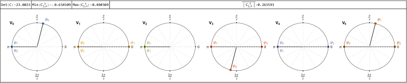
Figure 4: A good set of phases $\widetilde{\varphi}_{j,m}$ for each phase shift $V_{j}$. The important parameters of the $C$-matrix, such as average value of each element of the inverse $C^{-1}$, determinant, and minimum/maximum value are detailed in the figure above the visual phase representation. For the phase gate $V_{2}$ all phases $\varphi_{2,m}=\pi$.

We have numerically simulated the MLE reconstruction of an HW-reduce density matrix in a $2$-photon $3$-mode LON system. The phase shifts $\widehat{V}_{j}=\text{diag}(\exp(\operatorname{{\mathbbm{i}}}\widetilde{\varphi}_{j,0}),...\exp(\operatorname{{\mathbbm{i}}}\widetilde{\varphi}_{j,M-1}))$ are determined under the two condition above through

$$\{\widetilde{\varphi}_{j,m}\}_{j,m}=\operatorname*{arg\,max}_{\varphi_{j,m}}|\text{det}(C)|,\;\;\text{ subject to }\;\;|C[j,\bm{\bm{n}}]|\leq\delta$$ (94)

where $\delta$ is a small number. The phase shifts found by this procedure are illustrated in Fig. 4, we can observe a high degree of symmetry in the resulting phases, most of them being either $\varphi_{j,l}=0$ or $\varphi_{j,l}=\pi$.

References

• [1] P.ย Kok, W.ย J. Munro, K.ย Nemoto, T.ย C. Ralph, J.ย P. Dowling, and G.ย J. Milburn. Linear optical quantum computing with photonic qubits. Reviews of Modern Physics, 79:135โ€“174, 2007.
• [2] J.ย L. Oโ€™Brien. Optical quantum computing. Science, 318(5856):1567โ€“1570.
• [3] R.ย Raussendorf and H.ย J. Briegel. A one-way quantum computer. Physical Review Letters, 86:5188โ€“5191, 2001.
• [4] R.ย Raussendorf and H.ย J. Briegel. Computational model underlying the one-way quantum computer. Quant. Inf. Comp., 6:443, 2002.
• [5] R.ย Raussendorf, D.ย E. Browne, and H.ย J. Briegel. Measurement-based quantum computation on cluster states. Physical Review A, 68:022312, 2003.
• [6] P.ย Walther, K.ย J. Resch, T.ย Rudolph, E.ย Schenck, H.ย Weinfurter, V.ย Vedral, M.ย Aspelmeyer, and A.ย Zeilinger. Experimental one-way quantum computing. Nature, 434(7030):169โ€“176, 2005.
• [7] A.ย Fowler and K.ย Goyal. Topological cluster state quantum computing. 9(9&10):721โ€“738.
• [8] D.ย E. Browne and T.ย Rudolph. Resource-efficient linear optical quantum computation. Physical Review Letters, 95:010501, 2005.
• [9] D.ย Gottesman and I.ย L. Chuang. Demonstrating the viability of universal quantum computation using teleportation and single-qubit operations. Nature, 402:390โ€“393, 1999.
• [10] X.ย Liu, X.-M. Hu, T.-X. Zhu, C.ย Zhang, Y.-X. Xiao, J.-L. Miao, Z.-W. Ou, P.-Y. Li, B.-H. Liu, Z.-Q. Zhou, C.-F. Li, and G.-C. Guo. Nonlocal photonic quantum gates over 7.0 km. Nature Communications, 15(1).
• [11] E.ย Knill, R.ย Laflamme, and G.ย J. Milburn. A scheme for efficient quantum computation with linear optics. Nature, 409(6816):46โ€“52, 2001.
• [12] R.ย Okamoto, J.ย L. OBrien, H.ย F. Hofmann, and S.ย Takeuchi. Realization of a knill-laflamme-milburn controlled-not photonic quantum circuit combining effective optical nonlinearities. Proceedings of the National Academy of Sciences, 108(25):10067โ€“10071, 2011.
• [13] S.ย Aaronson. A linear-optical proof that the permanent isย #\#p-hard. Proceedings of the Royal Society of London A: Mathematical, Physical and Engineering Sciences, 467(2136):3393โ€“3405, 2011.
• [14] S.ย Aaronson and A.ย Arkhipov. The computational complexity of linear optics. In Proc. of the Forty-third Annual ACM Symposium on Theory of Computing, pages 333โ€“342. Association for Computing Machinery, 2011.
• [15] C.ย S. Hamilton, R.ย Kruse, L.ย Sansoni, S.ย Barkhofen, C.ย Silberhorn, and I.ย Jex. Gaussian boson sampling. Physical Review Letters, 119(17):170501, 2017.
• [16] H.-S. Zhong, H.ย Wang, Y.-H. Deng, M.-C. Chen, L.-C. Peng, Y.-H. Luo, J.ย Qin, D.ย Wu, X.ย Ding, Y.ย Hu, P.ย Hu, X.-Y. Yang, W.-J. Zhang, H.ย Li, Y.ย Li, X.ย Jiang, L.ย Gan, G.ย Yang, L.ย You, Z.ย Wang, L.ย Li, N.-L. Liu, C.-Y. Lu, and J.-W. Pan. Quantum computational advantage using photons. Science, 370(6523):1460โ€“1463, 2020.
• [17] H.-S. Zhong, Y.-H. Deng, J.ย Qin, H.ย Wang, M.-C. Chen, L.-C. Peng, Y.-H. Luo, D.ย Wu, S.-Q. Gong, H.ย Su, Y.ย Hu, P.ย Hu, X.-Y. Yang, W.-J. Zhang, H.ย Li, Y.ย Li, X.ย Jiang, L.ย Gan, G.ย Yang, L.ย You, Z.ย Wang, L.ย Li, N.-L. Liu, J.ย J. Renema, C.-Y. Lu, and J.-W. Pan. Phase-programmable gaussian boson sampling using stimulated squeezed light. Physical Review Letters, 127:180502, 2021.
• [18] J.ย C.ย F. Matthews, A.ย Politi, StefanovAndre, and J.ย L. Oโ€™Brien. Manipulation of multiphoton entanglement in waveguide quantum circuits. Nat Photon, 3(6):346โ€“350, 2009.
• [19] J.ย C.ย F. Matthews, A.ย Politi, D.ย Bonneau, and J.ย L. Oโ€™Brien. Heralding two-photon and four-photon path entanglement on a chip. Physical Review Letters, 107:163602, 2011.
• [20] J.ย Wang, S.ย Paesani, Y.ย Ding, R.ย Santagati, P.ย Skrzypczyk, A.ย Salavrakos, J.ย Tura, R.ย Augusiak, L.ย Manฤinska, D.ย Bacco, D.ย Bonneau, J.ย W. Silverstone, Q.ย Gong, A.ย Acรญn, K.ย Rottwitt, L.ย K. Oxenlรธwe, J.ย L. Oโ€™Brien, A.ย Laing, and M.ย G. Thompson. Multidimensional quantum entanglement with large-scale integrated optics. Science, 360(6386):285โ€“291, 2018.
• [21] X.-M. Hu, W.-B. Xing, B.-H. Liu, Y.-F. Huang, C.-F. Li, G.-C. Guo, P.ย Erker, and M.ย Huber. Efficient generation of high-dimensional entanglement through multipath down-conversion. Physical Review Letters, 125(9), 2020.
• [22] J.-Y. Wu and H.ย F. Hofmann. Evaluation of bipartite entanglement between two optical multi-mode systems using mode translation symmetry. New Journal of Physics, 19(10):103032, 2017.
• [23] J.-Y. Wu and M.ย Murao. Complementary properties of multiphoton quantum states in linear optics networks. New Journal of Physics, 22(10):103054, 2020.
• [24] T.ย Kiyohara, N.ย Yamashiro, R.ย Okamoto, H.ย Araki, J.-Y. Wu, H.ย F. Hofmann, and S.ย Takeuchi. Direct and efficient verification of entanglement between two multimodeโ€“multiphoton systems. Optica, 7(11):1517, 2020.
• [25] J.-Y. Wu. Generation and detection of discrete-variable multipartite entanglement with multirail encoding in linear-optics networks. Physical Review A, 106:032437, 2022.
• [26] D.ย F.ย V. James, P.ย G. Kwiat, W.ย J. Munro, and A.ย G. White. Measurement of qubits. Physical Review A, 64:052312, 2001.
• [27] R.ย T. Thew, K.ย Nemoto, A.ย G. White, and W.ย J. Munro. Qudit quantum-state tomography. Physical Review A, 66(1), 2002.
• [28] M.ย Paris and J.ย Rehacek. Quantum State Estimation. Springer Science & Business Media.
• [29] L.ย Banchi, W.ย S. Kolthammer, and M.ย S. Kim. Multiphoton tomography with linear optics and photon counting. Physical Review Letters, 121:250402, 2018.
• [30] Normally, the state prepared for LOQC should not have a too large photon number relative to the mode number, otherwise, the success probability will decrease dramatically.
• [31] C.ย Taballione, M.ย C. Anguita, M.ย deย Goede, P.ย Venderbosch, B.ย Kassenberg, H.ย Snijders, N.ย Kannan, W.ย L. Vleeshouwers, D.ย Smith, J.ย P. Epping, R.ย vanย der Meer, P.ย W.ย H. Pinkse, H.ย vanย den Vlekkert, and J.ย J. Renema. 20-mode universal quantum photonic processor. Quantum, 7:1071.
• [32] H.ย Weyl. Quantenmechanik und gruppentheorie. Zeitschrift fรผr Physik, 46(1โ€“2):1โ€“46.
• [33] H.ย Weyl. The theory of groups and quantum mechanics. Courier Corporation, 1950.
• [34] J.ย Schwinger. Unitary operator bases. Proceedings of the National academy of Sciences of the United States of America, 46:570, 1960.
• [35] T.ย Durt, B.-G. Englert, I.ย Bengtsson, and K.ย ลปyczkowski. On mutually unbiased bases. International Journal of Quantum Information, 08(04):535โ€“640, 2010.
• [36] A.ย Asadian, P.ย Erker, M.ย Huber, and C.ย Klรถckl. Heisenberg-weyl observables: Bloch vectors in phase space. Phys. Rev. A, 94:010301, 2016.
• [37] A.ย M. Palici, T.-A. Isdraila, S.ย Ataman, and R.ย Ionicioiu. OAM tomography with heisenbergโ€“weyl observables. Quantum Science and Technology, 5(4):045004.
• [38] E.ย Knill and R.ย Laflamme. Power of one bit of quantum information. Physical Review Letters, 81:5672โ€“5675, 1998.
• [39] Z.ย Hradil. Quantum-state estimation. Phys. Rev. A, 55:R1561โ€“R1564, 1997.
• [40] Z.ย Hradil, J.ย ล˜ehรกฤek, J.ย Fiurรกลกek, and M.ย Jeลพek. Maximum-Likelihood Methodsin Quantum Mechanics, pages 59โ€“112. Springer Berlin Heidelberg, Berlin, Heidelberg, 2004.
• [41] J.ย B. Altepeter, D.ย F. James, and P.ย G. Kwiat. Qubit Quantum State Tomography, pages 113โ€“145. Springer Berlin Heidelberg, Berlin, Heidelberg, 2004.
• [42] Also referred to as the shift operator and clock operator, respectively, by some authors.
• [43] J.-Y. Wu. Adaptive state fidelity estimation for higher dimensional bipartite entanglement. Entropy, 22(8):886, 2020.
• [44] M.ย Karczewski, R.ย Pisarczyk, and P.ย Kurzyล„ski. Genuine multipartite indistinguishability and its detection via the generalized hong-ou-mandel effect. Physical Review A, 99(4):042102, 2019.
• [45] A.ย M. Minke, A.ย Buchleitner, and C.ย Dittel. Characterizing four-body indistinguishability via symmetries. New Journal of Physics, 23(7):073028.
• [46] J.ย Bavaresco, N.ย H. Valencia, C.ย Klรถckl, M.ย Pivoluska, P.ย Erker, N.ย Friis, M.ย Malik, and M.ย Huber. Measurements in two bases are sufficient for certifying high-dimensional entanglement. Nature Physics, 14(10):1032โ€“1037, 2018.