Integrated Minimum Mean Squared Error Algorithms for Combined Acoustic Echo Cancellation and Noise Reduction

Abstract

In many speech recording applications, noise and acoustic echo corrupt the desired speech. Consequently, combined noise reduction (NR) and acoustic echo cancellation (AEC) is required. Generally, a cascade approach is followed, i.e., the AEC and NR are designed in isolation by selecting a separate signal model, formulating a separate cost function, and using a separate solution strategy. The AEC and NR are then cascaded one after the other, not accounting for their interaction. In this paper, however, an integrated approach is proposed to consider this interaction in a general multi-microphone/multi-loudspeaker setup. Therefore, a single signal model of either the microphone signal vector or the extended signal vector, obtained by stacking microphone and loudspeaker signals, is selected, a single mean squared error cost function is formulated, and a common solution strategy is used. Using this microphone signal model, a multi-channel Wiener filter (MWF) is derived. Using the extended signal model, an extended MWF (MWF_ext) is derived, and several equivalent expressions are found, which nevertheless are interpretable as cascade algorithms. Specifically, the MWF_ext is shown to be equivalent to algorithms where the AEC precedes the NR (AEC-NR), the NR precedes the AEC (NR-AEC), and the extended NR (NR_ext) precedes the AEC and post-filter (PF) (NR_ext-AEC-PF). Under rank-deficiency conditions the MWF_ext is non-unique, such that this equivalence amounts to the expressions being specific, not necessarily minimum-norm solutions for this MWF_ext. The practical performances nonetheless differ due to non-stationarities and imperfect correlation matrix estimation, resulting in the AEC-NR and NR_ext-AEC-PF attaining best overall performance.

I Introduction

In many speech recording applications, e.g., hands-free telephony in a car or telecommunication using hearing instruments, noise and acoustic echo corrupt the desired speech [1] as illustrated in Fig. 1. The noise originates from within the room (the so-called near-end room), while the echo originates from loudspeakers playing signals recorded in another room (the so-called far-end room). To suppress the near-end room noise and echo, noise reduction (NR) and acoustic echo cancellation (AEC) algorithms are required.

Figure 1: Algorithms for combined acoustic echo cancellation (AEC) and noise reduction (NR) aim at providing an estimate of the desired speech $\hat{s}_{r}$ in reference microphone $r$ by suppressing the near-end room noise signal vector $\mathbf{n}$ and echo signal vector $\mathbf{e}$, originating from the loudspeaker signals $l_{j}$, $j\in\{1,\cdots,L\}$, by means of the echo path map $F(.)$. To this end, the microphone signal vector $\mathbf{m}$ and possibly the loudspeaker signals $l_{j}$ are utilised. The figurines have been generated using [2].

AEC aims at estimating the desired speech by suppressing the echo [1]. AEC algorithms traditionally exploit the availability of loudspeaker signals to compute an estimate of this echo, which can then be subtracted from the microphone signals [1]. Other approaches exist as well, such as single-channel gains [3], end-to-end neural networks [4], and combinations of traditional signal processing and neural networks [5].

NR aims at estimating the desired speech by suppressing the near-end room noise [6, 7]. NR algorithms traditionally exploit the availability of microphone signals. Examples of NR algorithms include beamformers, such as the multi-channel Wiener filter (MWF) and generalised sidelobe canceller (GSC) [6, 7], Kalman filters [8], single-channel gains [9], end-to-end neural networks [10] and combinations of traditional signal processing and neural networks [11].

Algorithms for combined AEC and NR consequently aim at estimating the desired speech by jointly suppressing the echo and near-end room noise [1]. Combined AEC and NR algorithms exploit the availability of microphone and loudspeaker signals as illustrated in Fig. 1. To achieve this combined AEC and NR, generally, a cascade approach is adhered to, i.e., the AEC and NR are designed in isolation by selecting a separate signal model, formulating a separate cost function, and using a separate solution strategy. The AEC and NR are then cascaded one after the other. This cascade approach leads to algorithms where the AEC precedes the NR (AEC-NR) [12, 13, 14], the NR precedes the AEC (NR-AEC) [15, 16, 17, 18], or variations thereof [19, 20, 21].

Despite the AEC being less perturbed by near-end room noise in the NR-AEC, the AEC-NR tends to outperform the NR-AEC in terms of echo suppression. Indeed, the AEC in the NR-AEC needs to track (the adaptivity of) the NR, which is not the case for the AEC in the AEC-NR [22, 16, 14]. Further, although the AEC needs to process the noisy microphone signal vectors, the AEC-NR can use the NR to suppress residual echo [23]. The NR-AEC, on the other hand, is advantageous computational-complexity-wise as only one echo path estimation per loudspeaker is required, opposed to one echo path estimation for each loudspeaker-microphone pair for the AEC-NR [22, 16, 14].

In this paper, the cascade approach is contrasted to an integrated approach where a single algorithm for joint AEC and NR is designed by selecting a single signal model, formulating a single cost function, and using a common solution strategy. Whereas the cascade approach, thus, designs two separate algorithms with distinct parameters, the integrated approach designs a single algorithm with shared parameters.

In [24, 25], this integrated approach has been applied using an extended signal model of stacked microphone and loudspeaker signal vectors, together with a linearly constrained minimum variance (LCMV) cost function. In [26], a combined state-space model for the echo path and the autoregressive desired speech has been considered, using a cost function and solution strategy based on Kalman filtering and expectation maximisation (EM). Integrated single-channel gain design has been studied in [27, 28, 29]. Neural networks, either combined with traditional signal processing algorithms [30] or end-to-end [31], have been investigated as well.

For specific choices of the signal model and cost function, the algorithms resulting from the cascade and integrated approaches can nevertheless be shown to be equivalent. In [12, 19, 32, 33, 34], a mean squared error (MSE) cost function has been used together with an extended signal model. While it is stressed that this integrated approach leads to a single algorithm with shared parameters for the AEC and NR, it has been shown that the resulting algorithm can be interpreted as the AEC-NR cascade algorithm in the $1$-microphone/$1$-loudspeaker setup [12, 19], in the $2$-microphone/$1$-loudspeaker setup with uncorrelated near-end room noise in both microphones [19], and in the multi-microphone/multi-loudspeaker setup when using a specific generalised eigenvalue decomposition (GEVD) implementation and (multiframe) linear signal model for the echo paths [34]. Similarly, in the multi-microphone/$1$-loudspeaker setup it has been shown that the resulting algorithm can be interpreted as an NR-AEC cascade algorithm [32], and in the multi-microphone/multi-loudspeaker as an extended MWF (MWF_ext), i.e., an MWF on an extended signal model when using the specific GEVD implementation and (multiframe) linear signal model [34]. Nevertheless, while both the AEC-NR, NR-AEC and MWF_ext are theoretically equivalent under these specific conditions, their practical performances differ due to parameter estimation differences, e.g., as described supra for the AEC-NR and NR-AEC.

The MSE cost has thus only been partially explored: only for specific choices of the signal model and cost function, and only showing equivalence for the AEC-NR, NR-AEC and MWF_ext. In this paper, the aim is to apply the integrated approach to the most general multi-microphone/multi-loudspeaker setup, where the loudspeaker and microphone signals are possibly linearly related, allowing to generalise previous work, to propose new algorithms, and to study practical performance differences across algorithms. Therefore, the main research questions, tackled in this paper are as follows:

1. What algorithms are retrieved by applying the integrated approach to a combined AEC and NR problem in the general multi-microphone/multi-loudspeaker setup, possibly with linear dependencies between the loudspeaker and microphone signals, and using an MSE cost function?

2. How do non-stationarities and imperfect correlation matrix estimation influence the practical performance of the algorithms?

As for the first research question, a single signal model of either the microphone signal vector, or the extended signal vector obtained by stacking microphone and loudspeaker signals will be selected, a single MSE cost function will be formulated, and a common solution strategy will be used. Selecting the microphone signal model, an MWF will be derived, whereas selecting the extended signal model, an extended MWF (MWF_ext) will be derived. This MWF_ext will be shown to be theoretically equivalent to several expressions, which turn out to be interpretable as specific cascade algorithms. Specifically, the MWF_ext will be shown to be equivalent to the AEC-NR and NR-AEC, thus generalising [12, 19, 32, 33, 34]. Further, the MWF_ext will be shown to be equivalent to an algorithm where an extended NR (NR_ext) precedes the AEC and a post-filter (PF) (NR_ext-AEC-PF) under the assumption of the echo paths being additive maps, i.e., preserving the addition operation. This algorithm without PF, NR_ext-AEC, has originally been proposed as a cascade algorithm for combined acoustic feedback cancellation (AFC) and NR [35], and as a cascade algorithm for combined AEC and NR [18]. In this paper, the algorithm will be adapted to the general AEC and NR problem, and the PF will be shown to be necessary for MSE optimality. Additionally, under rank-deficiency conditions the MWF_ext is non-unique, such that it will be shown that under these rank-deficiency conditions the theoretical equivalence of the AEC-NR, NR-AEC and NR_ext-AEC-PF expressions to the MWF_ext amounts to the expressions being specific, not necessarily minimum-norm solutions for this MWF_ext.

As for the second research question, non-stationarities and imperfect correlation matrix estimation effects will be analysed theoretically, and validated experimentally. The AEC-NR and NR_ext-AEC-PF will be shown to attain best overall performance.

In Section II the cascade approach is reviewed first, discussing the AEC and NR design in isolation. This is contrasted to the integrated approach in Section III. The practical performance differences due to non-stationarities and imperfect correlation matrix estimation are analysed theoretically in Section IV, and after introducing the simulation setup in Section V, also experimentally in Section VI. MATLAB code is available in [36]. Finally, Section VII draws the conclusions.

II Cascade approach

Section II-A and Section II-B describe the design of the isolated AEC and NR algorithms, optimal in the MSE sense for their isolated cost functions. The near-end room noise presence is thus neglected in the design of the AEC and the echo presence in the design of the NR. Section II-C considers the cascade approach for combined AEC and NR.

The signal model is presented in the $z$-domain to accommodate the duality between frequency domain and time domain. The conversion from $z$- to frequency domain is realised by replacing index $z$ with frequency-bin index $f$, and possibly frame index $k$. The conversion from $z$- to time domain is realised by replacing the $z$-domain variables with time-lagged vectors, possibly multiplied with Toeplitz matrices, and replacing index $z$ with time index $t$.

II-A Acoustic echo cancellation (AEC)

AEC aims at estimating the desired speech by suppressing the echo originating from the loudspeakers. To this end, the echo signals are estimated from the loudspeaker signals and subtracted from the microphone signals [1][37, Chapter 5].  

II-A1 Signal model

Considering an $M$-microphone/$L$-loudspeaker setup, the microphone signals $m_{i}(z)$, $i\in\{1,\cdots,M\}$, can be stacked into the microphone signal vector $\mathbf{m}(z)\in\mathbb{C}^{M\times 1}$ as

$$\mathbf{m}(z)=\begin{bmatrix}m_{1}(z)&m_{2}(z)&\cdots&m_{M}(z)\end{bmatrix}^{\top}_{\textstyle\raisebox{2.0pt}{.}}$$ (1)

This microphone signal vector can be decomposed into a desired speech signal vector $\mathbf{s}(z)\in\mathbb{C}^{M\times 1}$ and an echo signal vector $\mathbf{e}(z)\in\mathbb{C}^{M\times 1}$ as

$$\mathbf{m}(z)=\mathbf{s}(z)+\mathbf{e}(z)_{\textstyle\raisebox{2.0pt}{,}}$$ (2)

where $\mathbf{e}(z)$ originates from the loudspeaker signal vector $\mathbf{l}(z)$

$$\mathbf{l}(z)=\begin{bmatrix}l_{1}(z)&l_{2}(z)&\cdots&l_{L}(z)\end{bmatrix}^{\top}_{\textstyle\raisebox{2.0pt}{}}$$ (3)

by means of a map $F(.):\mathbb{C}^{L\times 1}\rightarrow\mathbb{C}^{M\times 1}$, i.e., $\mathbf{e}(z)=F(\mathbf{l}(z))$. While $F(.)$ can be a general map, it can also be restricted by, e.g., assuming $F(.)$ to be an additive or linear map. If the loudspeaker signal vector $\mathbf{l}(z)$ consists of a far-end room speech component $\mathbf{l}^{s}(z)$ and a far-end room noise component $\mathbf{l}^{n}(z)$, an additive map preserves this speech-noise relation as [18]

$$\mathbf{e}(z) =F(\mathbf{l}^{s}(z)+\mathbf{l}^{n}(z))=F(\mathbf{l}^{s}(z))+F(\mathbf{l}^{n}(z))$$ (4a)

$$=\mathbf{e}^{s}(z)+\mathbf{e}^{n}(z)_{\textstyle\raisebox{2.0pt}{,}}$$ (4b)

with $\mathbf{e}^{s}(z)$ and $\mathbf{e}^{n}(z)$ the far-end room speech and noise components in the echo respectively. In a linear map,

$$\mathbf{e}(z) =F\left(\mathbf{l}(z)\right)$$ (5a)

$$=F_{\text{lin}}(z)\mathbf{l}(z)_{\textstyle\raisebox{2.0pt}{,}}$$ (5b)

with

$$F_{\text{lin}}(z)=\begin{bmatrix}f_{1}^{1}(z)&\cdots&f_{1}^{L}(z)\\ \vdots&\ddots&\vdots\\ f_{M}^{1}(z)&\cdots&f_{M}^{L}(z)\end{bmatrix}_{\textstyle\raisebox{0.0pt}{,}}$$ (6)

and $f_{i}^{j}(z)$ the transfer function of the echo path between the $j$th loudspeaker and the $i$th microphone. A continuous-time linear echo path combined with multi-rate digital signal processing (with aliasing), e.g., corresponds to an additive map rather than a linear map.  

II-A2 Cost function

The goal of the AEC is to minimise the MSE between the echo signal for a chosen reference microphone $r\in\{1,\cdots,M\}$ and the filtered loudspeaker signal vector $\mathbf{w}_{\text{AEC}}(z)^{H}\mathbf{l}(z)$, with $\mathbf{w}_{\text{AEC}}(z)\in\mathbb{C}^{L\times 1}$ [37, Chapter 5]:

$$\mathbf{w}_{\text{AEC}}(z)=\operatorname*{argmin}_{\mathbf{w}(z)}\mathbb{E}\left\{\left\lVert e_{r}(z)-\mathbf{w}(z)^{H}\mathbf{l}(z)\right\rVert^{2}_{2}\right\}_{\textstyle\raisebox{2.0pt}{.}}$$ (7)

II-A3 Solution strategy

Defining $R_{ll}(z)=\mathbb{E}\left\{\mathbf{l}(z)\mathbf{l}(z)^{H}\right\}\in\mathbb{C}^{L\times L}$ and $R_{le}(z)$
$=\mathbb{E}\left\{\mathbf{l}(z)\mathbf{e}(z)^{H}\right\}\in\mathbb{C}^{L\times M}$ as the loudspeaker correlation matrix and the loudspeaker-echo cross-correlation matrix respectively, the solution to (7) is given as the solution to the Wiener-Hopf equations [37, Chapter 5]

$$R_{ll}(z)\mathbf{w}_{\text{AEC}}(z)=R_{{le}}(z)\mathbf{t}_{r_{\textstyle\raisebox{2.0pt}{,}}}$$ (8)

with $\mathbf{t}_{r}\in\mathbb{C}^{M\times 1}$ a unit vector with $1$ at position $r$ and $0$ elsewhere. The solution to (8) is given as

$$\mathbf{w}_{\text{AEC}}(z)=R_{ll}(z)^{g}R_{{le}}(z)\mathbf{t}_{r_{\textstyle\raisebox{2.0pt}{,}}}$$ (9)

with $.^{g}$ denoting the generalised inverse^, [38]. This generalised inverse is non-unique if $R_{ll}(z)$ is rank-deficient, although specific choices can be made such as the pseudo-inverse $.^{\dagger}$ which is uniquely defined, and with which (9) corresponds to the minimum-norm solution [39]. If $R_{ll}(z)$ is full-rank, i.e., the loudspeaker signals are linearly independent, then $.^{g}$ can be replaced with the inverse $.^{-1}$.

The desired speech estimate $\hat{s}_{r,\text{AEC}}\in\mathbb{C}$ in microphone $r$ is given as [37, Chapter 5]

$$\hat{s}_{r,\text{AEC}}(z)=\mathbf{t}_{r}^{H}\mathbf{m}(z)-\mathbf{w}_{{AEC}}(z)^{H}\mathbf{l}(z)_{\textstyle\raisebox{2.0pt}{.}}$$ (10)

Depending on possible post-processing of the signals after applying the AEC, this procedure can be repeated for multiple choices of reference microphone.

II-B Noise reduction (NR)

NR aims at estimating the desired speech by suppressing the near-end room noise through filtering the microphone signals [6].  

II-B1 Signal model

Considering an $M$-microphone setup, the microphone signal vector $\mathbf{m}(z)\in\mathbb{C}^{M\times 1}$ consists of a desired speech signal vector $\mathbf{s}(z)\in\mathbb{C}^{M\times 1}$ and a near-end room noise signal vector $\mathbf{n}(z)\in\mathbb{C}^{M\times 1}$

$$\mathbf{m}(z)=\mathbf{s}(z)+\mathbf{n}(z)_{\textstyle\raisebox{2.0pt}{.}}$$ (11)

II-B2 Cost function

The goal of the NR is to minimise the MSE between the desired speech signal for a chosen reference microphone $r\in\{1,\cdots,M\}$ and the filtered microphone signal vector $\mathbf{w}_{\text{NR}}(z)^{H}\mathbf{m}(z)$, with $\mathbf{w}_{\text{NR}}(z)\in\mathbb{C}^{M\times 1}$ [6, 40]:

$$\mathbf{w}_{\text{NR}}(z)=\operatorname*{argmin}_{\mathbf{w}(z)}\mathbb{E}\left\{\left\lVert s_{r}(z)-\mathbf{w}(z)^{H}\mathbf{m}(z)\right\rVert_{2}^{2}\right\}_{\textstyle\raisebox{2.0pt}{.}}$$ (12)

II-B3 Solution strategy

Defining $R_{mm}(z)=\mathbb{E}\left\{\mathbf{m}(z)\mathbf{m}(z)^{H}\right\}\in\mathbb{C}^{M\times M}$ and $R_{ss}(z)=\mathbb{E}\left\{\mathbf{s}(z)\mathbf{s}(z)^{H}\right\}\in\mathbb{C}^{M\times M}$ as the microphone correlation matrix and the desired speech correlation matrix respectively, and assuming $\mathbf{s}(z)$ and $\mathbf{n}(z)$ to be uncorrelated, the solution to (12) is given as [6]

$$\mathbf{w}_{\text{NR}}(z)=R_{mm}(z)^{g}R_{ss}(z)\mathbf{t}_{r_{\textstyle\raisebox{2.0pt}{.}}}$$ (13)

If $R_{mm}(z)$ is rank-deficient, then $.^{g}$ can again be chosen as $.^{\dagger}$, such that (13) corresponds to the minimum-norm solution. Indeed, $R_{mm}(z)$ can be rank-deficient, e.g., modelling $<M$ localised noise sources. If $R_{mm}(z)$ is full-rank, then $.^{g}$ can be replaced with $.^{-1}$. The desired speech estimate $\hat{s}_{r,\text{NR}}(z)\in\mathbb{C}$ in microphone $r$ is given as [6]

$$\hat{s}_{r,\text{NR}}(z)=\mathbf{w}_{\text{NR}}(z)^{H}\mathbf{m}(z)_{\textstyle\raisebox{2.0pt}{.}}$$ (14)

Depending on possible post-processing of the signals after applying the NR, this procedure can be repeated for multiple choices of reference microphone.

II-C Combined AEC and NR

To resolve the combined AEC and NR problem, both algorithms are cascaded one after the other, where the AEC precedes the NR (AEC-NR) [12, 13, 14], the NR precedes the AEC (NR-AEC) [15, 16, 17, 18] or variations thereof are considered [19, 20, 21]. As such, the cascade approach may suffer from algorithmic conflicts as the interaction between the isolated algorithms is not taken into account. Indeed, (residual) echo and near-end room noise may leak between the different stages of the cascade algorithms, thereby reducing performance.

III Integrated approach

In this section, the integrated approach is applied by selecting a signal model, including both the near-end room noise and echo, of either the microphone signal vector only or of an extended signal vector obtained by stacking microphone and loudspeaker signals (Section III-A), formulating an MSE cost function (Section III-B), and using a common solution strategy (Section III-C). Using the microphone signal model, an MWF will be obtained, whereas using the extended signal model an MWF_ext will be obtained. Subsequently, several theoretically equivalent expressions to the MWF_ext are derived, which turn out to be nevertheless interpretable as specific cascade algorithms, as illustrated in Fig. 2. Specifically, the MWF_ext is shown to be theoretically equivalent to algorithms where the AEC precedes the NR (AEC-NR), the NR precedes the AEC (NR-AEC), and the extended NR (NR_ext) precedes the AEC and a post-filter (PF) (NR_ext-AEC-PF). Under rank-deficiency conditions the MWF_ext is non-unique, such that this theoretical equivalence amounts to the expressions being specific, not necessarily minimum-norm solutions for this MWF_ext.

For conciseness, the $z$-indices will be omitted from now on.

(a) MWF

(b) MWF_ext

(c) AEC-NR

(d) NR-AEC

(e) NR_ext-AEC-PF

Figure 2: Cascade interpretation of the integrated algorithms. (a) The MWF is obtained using the microphone signal model. (b) The MWF_ext is obtained using the extended signal model, which can be shown to be theoretically equivalent to (c) the AEC-NR, (d) the NR-AEC, and (e) the NR_ext-AEC-PF.

III-A Signal model

The microphone signal vector $\mathbf{m}\in\mathbb{C}^{M\times 1}$ is defined as a mixture of a desired speech signal vector $\mathbf{s}\in\mathbb{C}^{M\times 1}$, an echo signal vector $\mathbf{e}\in\mathbb{C}^{M\times 1}$ and a near-end room noise signal vector $\mathbf{n}\in\mathbb{C}^{M\times 1}$:

$$\begin{IEEEeqnarraybox}[]{rll}\mathbf{m}&=\mathbf{s}+\mathbf{e}+\mathbf{n}_{\textstyle\raisebox{2.0pt}{.}}\end{IEEEeqnarraybox}$$ (15)

This signal model (15) will be used to derive the MWF in Section III-C1.

An extended signal model can be constructed as well, stacking the microphone signal vector $\mathbf{m}$ and loudspeaker signal vector $\mathbf{l}$ into $\tilde{\mathbf{m}}\in\mathbb{C}^{(M+L)\times 1}$ as

$$\tilde{\mathbf{m}} =\begin{bmatrix}\mathbf{m}^{\top}&\mathbf{l}^{\top}\end{bmatrix}^{\top}$$ (16a)

$$=\tilde{\mathbf{s}}+\tilde{\mathbf{e}}+\tilde{\mathbf{n}}$$ (16b)

$$=\begin{bmatrix}\mathbf{s}\\ \mathbf{0}_{L\times 1}\end{bmatrix}+\begin{bmatrix}\mathbf{e}\\ \mathbf{l}\end{bmatrix}+\begin{bmatrix}\mathbf{n}\\ \mathbf{0}_{L\times 1}\end{bmatrix}_{\textstyle\raisebox{2.0pt}{,}}$$ (16c)

Herein, $\mathbf{0}_{L\times 1}\in\mathbb{C}^{L\times 1}$ corresponds to a vector containing only zero elements. This signal model (16) will be used to derive the AEC-NR and NR-AEC in Section III-C3 and Section III-C4 respectively.

If the echo path is an additive map as well, $\mathbf{e}$ can be decomposed into the sum of far-end room speech and noise components, i.e., $\mathbf{e}^{s}$ and $\mathbf{e}^{n}$, originating from $\mathbf{l}^{s}$ and $\mathbf{l}^{n}$ respectively, such that (15) and (16) can be decomposed into

$$\mathbf{m}=\mathbf{s}+\mathbf{e}^{s}+\mathbf{e}^{n}+\mathbf{n}_{\textstyle\raisebox{2.0pt}{,}}$$ (17)

and

$$\tilde{\mathbf{m}} =\tilde{\mathbf{s}}+\tilde{\mathbf{e}}^{s}+\tilde{\mathbf{e}}^{n}+\tilde{\mathbf{n}}$$ (18a)

$$=\begin{bmatrix}\mathbf{s}\\ \mathbf{0}_{L\times 1}\end{bmatrix}+\begin{bmatrix}\mathbf{e}^{s}\\ \mathbf{l}^{s}\end{bmatrix}+\begin{bmatrix}\mathbf{e}^{n}\\ \mathbf{l}^{n}\end{bmatrix}+\begin{bmatrix}\mathbf{n}\\ \mathbf{0}_{L\times 1}\end{bmatrix}_{\textstyle\raisebox{2.0pt}{.}}$$ (18b)

The signal model (16) will be used to derive the NR_ext-AEC-PF in Section III-C5.

As $\mathbf{s}$ and $\mathbf{e}^{s}$ represent speech signal vectors, they can be assumed to attain an on-off behaviour. To detect these on-off periods, voice activity detectors (VADs) are assumed to be available, i.e., $\text{VAD}_{s}$ and $\text{VAD}_{e^{s}}$ differentiate between on-off periods in $\mathbf{s}$ and $\mathbf{e}^{s}$ respectively. As $\mathbf{n}$ and $\mathbf{e}^{n}$, on the other hand, represent noise signal vectors, they can be assumed to be always-on. Thus, the following regimes can be defined:

• $\text{VAD}_{s}=1$, $\text{VAD}_{e^{s}}=1$: $\mathbf{m}=\mathbf{s}+\mathbf{e}+\mathbf{n}$ recorded,

• $\text{VAD}_{s}=1$, $\text{VAD}_{e^{s}}=0$: $\mathbf{s}+\mathbf{e}^{n}+\mathbf{n}$ recorded,

• $\text{VAD}_{s}=0$, $\text{VAD}_{e^{s}}=1$: $\mathbf{e}+\mathbf{n}$ recorded,

• $\text{VAD}_{s}=0$, $\text{VAD}_{e^{s}}=0$: $\mathbf{e}^{n}+\mathbf{n}$ recorded.

For general non-additive echo path maps, $\text{VAD}_{e^{s}}$ then does not detect on-off periods of $\mathbf{e}^{s}$ itself as possibly only non-linear combinations of the loudspeaker signals can be observed, but $\text{VAD}_{e^{s}}$ then still discriminates between activity of all components in the echo signal and activity of only partial components. In the literature (e.g., [33, 25]), the echo is often assumed to only contain a stationary always-on signal, which corresponds to only keeping $\mathbf{e}^{n}$ and discarding $\text{VAD}_{e^{s}}$.

Further, the following assumptions are made:

• $\mathbf{s}$, $\mathbf{n}$, $\mathbf{e}^{s}$ and $\mathbf{e}^{n}$ are uncorrelated, $\mathbf{l}^{s}$ and $\mathbf{l}^{n}$ are uncorrelated, and $\mathbf{l}^{s}$ and $\mathbf{l}^{n}$ are uncorrelated with $\mathbf{s}$ and $\mathbf{n}$.

• For the theoretical derivation all (speech) signals will be assumed stationary during their on periods. However, in Section IV, this assumption will be relaxed by considering the influence of non-stationary signal vectors. Indeed, in practice, $\mathbf{s}$ (and $\mathbf{e}^{s}$) are non-stationary, whereas $\mathbf{n}$ (and $\mathbf{e}^{n}$) are nevertheless considered to be stationary.

The general $M$-microphone/$L$-loudspeaker setup is considered, and no assumptions are made regarding the rank of $R_{ss}$, $R_{nn}$, $R_{mm}$ or $R_{ll}$, thus possibly modelling localised desired speech and near-end room noise sources and linearly related loudspeaker and microphone signals.

III-B Cost function

The goal of the integrated AEC and NR algorithm is to minimise the MSE between the desired speech signal ${s}_{r}\in\mathbb{C}$ and a filtered signal vector, simultaneously suppressing the echo signal vector $\mathbf{e}$ and near-end room noise signal vector $\mathbf{n}$, by either considering the microphone signal model (15), i.e.,

$$\mathbf{w}_{\text{int}}=\operatorname*{argmin}_{\mathbf{w}}\mathbb{E}\left\{\left\lVert s_{r}-\mathbf{w}^{H}\mathbf{m}\right\rVert_{2}^{2}\right\}_{\textstyle\raisebox{2.0pt}{,}}$$ (19)

to design $\mathbf{w}_{\text{int}}\in\mathbb{C}^{M\times 1}$, or the extended signal model (16), i.e.,

$$\begin{IEEEeqnarraybox}[]{rll}\tilde{\mathbf{w}}_{\text{int}}&=\operatorname*{argmin}_{\tilde{\mathbf{w}}}\mathbb{E}\left\{\left\lVert s_{r}-\tilde{\mathbf{w}}^{H}\tilde{\mathbf{m}}\right\rVert_{2}^{2}\right\}_{\textstyle\raisebox{2.0pt}{,}}\end{IEEEeqnarraybox}$$ (20)

to design $\tilde{\mathbf{w}}_{\text{int}}\in\mathbb{C}^{\left(M+L\right)\times 1}$. As illustrated in Fig. 1, the loudspeaker signals are only filtered by $\tilde{\mathbf{w}}_{\text{int}}$ when estimating $s_{r}$, thus without affecting the playback in the near-end room.

III-C Solution strategy

III-C1 Multi-channel Wiener filter (MWF)

Using the microphone signal model (15), the solution to (19) is obtained as

$$\boxed{\begin{IEEEeqnarraybox}[]{rll}\mathbf{w}_{\text{int}}&=R_{{m}{m}}^{g}R_{s{s}}{{\mathbf{t}}_{r}}_{\textstyle\raisebox{2.0pt}{,}}\end{IEEEeqnarraybox}}$$ (21)

hence corresponding to the multi-channel Wiener filter (MWF) (Fig. 2(a)). $R_{mm}=R_{ss}+R_{ee}+R_{nn}$ can be computed during periods of desired speech and echo activity ($\text{VAD}_{s}=1\land\text{VAD}_{e^{s}}=1$). $R_{ss}$ can be computed by constructing $R_{nn}+R_{ee}$ during periods of simultaneous desired speech inactivity and echo activity ($\text{VAD}_{s}=0\land\text{VAD}_{e^{s}}=1$), and subtracting the result from $R_{mm}$.  

III-C2 Extended multi-channel Wiener filter (MWF_ext)

Similar to the MWF, using the extended signal model (16), the solution to (20) is obtained as an MWF with extended correlation matrices $R_{\tilde{m}\tilde{m}}=\mathbb{E}\left\{\tilde{\mathbf{m}}\tilde{\mathbf{m}}^{H}\right\}\in\mathbb{C}^{\left(M+L\right)\times\left(M+L\right)}$ and $R_{\tilde{s}\tilde{s}}=\mathbb{E}\left\{\tilde{\mathbf{s}}\tilde{\mathbf{s}}^{H}\right\}\in\mathbb{C}^{\left(M+L\right)\times\left(M+L\right)}$

$$\boxed{\begin{IEEEeqnarraybox}[]{rll}\tilde{\mathbf{w}}_{\text{int}}&=R_{\tilde{m}\tilde{m}}^{g}R_{\tilde{s}\tilde{s}}\tilde{\mathbf{t}}_{r_{\textstyle\raisebox{2.0pt}{,}}}\end{IEEEeqnarraybox}}$$ (22)

hence, named the extended MWF (MWF_ext) (Fig. 2(b)). $R_{\tilde{m}\tilde{m}}$ can be computed when $\text{VAD}_{s}=1\land\text{VAD}_{e^{s}}=1$, while $R_{\tilde{s}\tilde{s}}$ can be computed by constructing $R_{\tilde{e}\tilde{e}}+R_{\tilde{n}\tilde{n}}$ when $\text{VAD}_{s}=0\land\text{VAD}_{e^{s}}=1$ and subtracting the result from $R_{\tilde{m}\tilde{m}}$.  

III-C3 AEC precedes NR (AEC-NR)

A closed-form expression for a valid generalised matrix inverse in (22) is as follows (cfr. Supplementary material Section 8)

$$\begin{IEEEeqnarraybox}[]{rll}&R_{\tilde{m}\tilde{m}}^{g,g}=\begin{bmatrix}\Sigma_{mm}^{\dagger}&-\Sigma_{mm}^{\dagger}R_{el}R_{ll}^{\dagger}\\ -R_{ll}^{\dagger}R_{le}\Sigma_{mm}^{\dagger}&R_{ll}^{\dagger}+R_{ll}^{\dagger}R_{le}\Sigma_{mm}^{\dagger}R_{el}R_{ll}^{\dagger}\end{bmatrix}_{\textstyle\raisebox{2.0pt}{,}}\end{IEEEeqnarraybox}$$ (23)

with $\Sigma_{mm}=R_{mm}-R_{el}R_{ll}^{\dagger}R_{le}$. Herein, $R_{\tilde{m}\tilde{m}}^{g,g}\in\mathbb{C}^{(M+L)\times(M+L)}$ is thus one possible valid expression for all of the generally non-unique generalised inverses $R_{\tilde{m}\tilde{m}}^{g}$ (cfr. Supplementary material Section 8). If $\Sigma_{mm}$ is full-rank, i.e., $\text{rank}\!\left(\Sigma_{mm}\right)=M$, then (23) corresponds to the pseudo-inverse. If additionally $\text{rank}\!\left(R_{ll}\right)=L$, then (23) corresponds to the inverse.

Plugging (23) into (22), the following expression is obtained, with $\mathbb{I}_{M\times M}\in\mathbb{C}^{M\times M}$ the identity matrix:

$$\boxed{\begin{IEEEeqnarraybox}[]{rll}&\tilde{\mathbf{w}}_{\text{int}}=\underbrace{\begin{bmatrix}\mathbb{I}_{M\times M}&0_{M\times L}\\ -R_{ll}^{\dagger}R_{le}&0_{L\times L}\end{bmatrix}}_{\text{AEC}}\underbrace{\begin{bmatrix}\Sigma_{mm}^{\dagger}R_{ss}\\ {0}_{L\times M}\end{bmatrix}}_{\text{NR}}{{\mathbf{t}}_{r_{\textstyle\raisebox{15.0pt}{,}}}}\end{IEEEeqnarraybox}}$$ (24)

which can be interpreted as an AEC preceding an NR (Fig. 2(c)). Indeed, $R_{ll}^{\dagger}R_{le}$ corresponds to the minimum-norm estimate of the echo paths as described in Section II-A. Furthermore, $\Sigma_{mm}$ can be interpreted as the microphone correlation matrix after applying the AEC, such that $\Sigma_{mm}^{\dagger}R_{ss}$ corresponds to an MWF aimed at suppressing near-end room noise and residual echo after the AEC. To show this equivalence, the microphone correlation matrix after applying the AEC is defined as

$$\begin{IEEEeqnarraybox}[]{rll}&\mathbb{E}\left\{\left(\mathbf{m}-R_{el}R_{ll}^{\dagger}\mathbf{l}\right)\left(\mathbf{m}-R_{el}R_{ll}^{\dagger}\mathbf{l}\right)^{H}\right\}\\ &=R_{mm}-2R_{el}R_{ll}^{\dagger}R_{le}+R_{el}R_{ll}^{\dagger}R_{ll}R_{ll}^{\dagger}R_{le_{\textstyle\raisebox{2.0pt}{,}}}\end{IEEEeqnarraybox}$$ (25)

wherein, $R_{ll}^{\dagger}R_{ll}R_{ll}^{\dagger}=R_{ll}^{\dagger}$ as per definition of the pseudo-inverse [39], such that (25) is indeed equal to $\Sigma_{mm}$. Consequently, if $\text{rank}\!\left(\Sigma_{mm}\right)=M$, then the MWF_ext (22) is uniquely defined and equivalent to the AEC-NR (24) as (23) then corresponds to the uniquely-defined pseudo-inverse. If $\text{rank}\!\left(\Sigma_{mm}\right)<M$, (22) is not uniquely defined as $R_{\tilde{m}\tilde{m}}^{g}$ is not unique. Nevertheless, (24) then still corresponds to one of the solutions of the Wiener-Hopf equations $R_{\tilde{m}\tilde{m}}\tilde{\mathbf{w}}=R_{\tilde{s}\tilde{s}}\tilde{\mathbf{t}}_{r}$, be it not necessarily to the minimum-norm solution.

To compute the correlation matrices in (24), $R_{ll}$ and $R_{le}$ can be readily constructed when $\text{VAD}_{e^{s}}=1$ as $\mathbf{s}$, $\mathbf{n}$ and $\mathbf{e}$ are uncorrelated, although in practice $R_{le}$ is computed when $\text{VAD}_{s}=0\land\text{VAD}_{e^{s}}=1$ to reduce excess error from $\mathbf{s}$ [37, Chapter 8]. $\Sigma_{mm}$ can then be constructed by computing the microphone correlation matrix after applying the AEC when $\text{VAD}_{s}=1\land\text{VAD}_{e^{s}}=1$, whereas $R_{ss}$ can be computed by subtracting the microphone correlation matrix after applying the AEC when $\text{VAD}_{s}=0\land\text{VAD}_{e^{s}}=1$, i.e., subtracting $R_{ee}+R_{nn}-R_{el}R_{ll}^{\dagger}R_{le}$, from $\Sigma_{mm}$.

If the echo path is linear and the AEC filters are chosen sufficiently long to model this echo path, i.e., $\mathbf{e}=F_{\text{lin}}\mathbf{l}$ and $R_{le}=R_{ll}F_{\text{lin}}^{H}$, $\tilde{\mathbf{w}}_{\text{int}}$ (24) is equivalent to $\tilde{\mathbf{w}}_{\text{int,lin}}\in\mathbb{C}^{\left(M+L\right)\times 1}$:

$$\boxed{\tilde{\mathbf{w}}_{\text{int,lin}}=\underbrace{\begin{bmatrix}\mathbb{I}_{M\times M}&0_{M\times L}\\ -R_{ll}^{\dagger}R_{ll}F_{\text{lin}}^{H}&0_{L\times L}\end{bmatrix}}_{\text{AEC}}\underbrace{\begin{bmatrix}\left(R_{ss}+R_{nn}\right)^{-1}R_{ss}\\ {0}_{L\times M}\end{bmatrix}}_{\text{NR}}{{\mathbf{t}}_{r_{\textstyle\raisebox{15.0pt}{,}}}}}$$ (26)

where the NR does not need to suppress residual echo as the AEC already fully cancels the echo. If $R_{ll}$ is full-rank, then $R_{ll}^{\dagger}R_{ll}F_{\text{lin}}=F_{\text{lin}}$, corresponding to straightforward AEC. If $R_{ll}$ is rank-deficient, i.e., if the loudspeaker signals are linearly dependent, the AEC $R_{ll}^{\dagger}R_{ll}F^{H}$ does not correspond to the true echo path matrix $F_{\text{lin}}$, but to a weighted version thereof. This linear weighting results in a far-end room dependence of the AEC, as $R_{ll}$ depends on the far-end room scenario. The AEC, therefore, also needs to adapt to changes in the far-end room, such that (26) provides a generalised expression for the multi-channel AEC problem, e.g., extending [41].  

III-C4 NR precedes AEC (NR-AEC)

By reordering the block matrices in (24), the following expression is obtained

$${\begin{IEEEeqnarraybox}[]{rll}&\tilde{\mathbf{w}}_{\text{int}}=\underbrace{\begin{bmatrix}\Sigma_{mm}^{\dagger}R_{ss}&0_{M\times L}\\ 0_{L\times M}&\mathbb{I}_{L\times L}\end{bmatrix}}_{\text{NR}}\underbrace{\begin{bmatrix}\mathbb{I}_{M\times M}\\ -R_{ll}^{\dagger}R_{le}\left(\Sigma_{mm}^{\dagger}R_{ss}\right)\end{bmatrix}}_{\text{AEC}}{\mathbf{t}}_{r_{\textstyle\raisebox{2.0pt}{.}}}\end{IEEEeqnarraybox}}$$ (27)

Here, the NR aimed to suppress the noise and residual echo now precedes the AEC (Fig. 2(d)), as opposed to the AEC-NR (24). As the echo signal vector after applying the NR is affected by the NR, the AEC not only has to model the echo paths but rather the combination of the echo paths and the NR, which leads to the additional factor $\Sigma_{mm}^{\dagger}R_{ss}$ in the AEC.

The advantage performance-wise of the NR-AEC over the AEC-NR is that the AEC operates under reduced near-end room noise influence, thereby using a cascade implementation where the NR precedes the AEC. However, to do so, the loudspeaker correlation matrix and the loudspeaker-echo cross-correlation matrix are only computed after applying an NR, such that $\Sigma_{mm}$ is generally replaced by $R_{mm}$, resulting in an expression $\tilde{\mathbf{w}}_{\text{mod}}\in\mathbb{C}^{\left(M+L\right)\times 1}$ with a modified NR and AEC, NR_mod and AEC_mod respectively [15, 16, 17, 18],

$$\boxed{\begin{IEEEeqnarraybox}[]{rll}&\tilde{\mathbf{w}}_{\text{mod}}=\underbrace{\begin{bmatrix}R_{mm}^{\dagger}R_{ss}&0_{M\times L}\\ 0_{L\times M}&\mathbb{I}_{L\times L}\end{bmatrix}}_{\text{NR\textsubscript{mod}}}\underbrace{\begin{bmatrix}\mathbb{I}_{M\times M}\\ -R_{ll}^{\dagger}R_{le}\left(R_{mm}^{\dagger}R_{ss}\right)\end{bmatrix}}_{\text{AEC\textsubscript{mod}}}{\mathbf{t}}_{r_{\textstyle\raisebox{2.0pt}{,}}}\end{IEEEeqnarraybox}}$$ (28)

which then loses its MSE optimality. $R_{mm}$ is computed when $\text{VAD}_{s}=1\land\text{VAD}_{e^{s}}=1$, and $R_{ss}$ is computed by subtracting $R_{ee}+R_{nn}$, collected when $\text{VAD}_{s}=0\land\text{VAD}_{e^{s}}=1$, from $R_{mm}$. $R_{ll}$ and $R_{le}\left(R_{mm}^{\dagger}R_{ss}\right)$ are then computed as the loudspeaker correlation matrix and the loudspeaker-echo cross-correlation matrix after applying the NR_mod.  

III-C5 Extended NR precedes AEC and PF (NR_ext-AEC-PF)

The additional assumption is now made that the echo path is an additive map, hence using the signal model (18). Furthermore, assume that $R_{ll}^{\dagger}R_{le}$ is a solution of the Wiener-Hopf equations $R_{l^{s}l^{s}}W=R_{l^{s}e^{s}}$, i.e., $R_{l^{s}l^{s}}R_{ll}^{\dagger}R_{le}=R_{l^{s}e^{s}}$. The latter assumption corresponds to the minimum-norm echo path estimate using the loudspeaker signals also being a solution of the Wiener-Hopf equations for the echo path estimate using only the far-end room speech component in the loudspeaker signals, thereby extending the assumption in [18] to the case where $R_{ll}$ and $R_{l^{s}l^{s}}$ can be rank-deficient.

Under these assumptions, an NR_ext filter $W_{\text{NR\textsubscript{ext}}}\in\mathbb{C}^{\left(M+L\right)\times\left(M+L\right)}$ can be defined as the MSE-optimal filter to suppress both $\tilde{\mathbf{n}}$ and $\tilde{\mathbf{e}}^{n}$ while preserving both $\tilde{\mathbf{s}}$ and $\tilde{\mathbf{e}}^{s}$:

$$W_{\text{NR\textsubscript{ext}}}=R_{\tilde{m}\tilde{m}}^{g,g}\left(R_{\tilde{s}\tilde{s}}+R_{\tilde{e}^{s}\tilde{e}^{s}}\right)_{\textstyle\raisebox{2.0pt}{.}}$$ (29)

Applying $W_{\text{NR\textsubscript{ext}}}$ to $\tilde{\mathbf{m}}$ leads to an extended signal vector,

$$\tilde{\mathbf{m}}^{`}=\begin{bmatrix}\mathbf{m}^{`}\\ \mathbf{l}^{`}\end{bmatrix}=W_{\text{NR\textsubscript{ext}}}^{H}\tilde{\mathbf{m}}_{\textstyle\raisebox{2.0pt}{.}}$$ (30)

Using (29) and the assumption that $R_{l^{s}l^{s}}R_{ll}^{\dagger}R_{le}=R_{l^{s}e^{s}}$, the following filter can be shown to be equivalent to (22) if $R_{\tilde{m}\tilde{m}}^{g,g}$ is chosen as defined in (23) for $R_{\tilde{m}\tilde{m}}^{g}$ both in (22) and (31) (cfr. Supplementary material Section 9)

$$\boxed{\begin{IEEEeqnarraybox}[]{rll}\tilde{\mathbf{w}}_{\text{int}}{=}&\underbrace{R_{\tilde{m}\tilde{m}}^{g,g}\left(R_{\tilde{s}\tilde{s}}+R_{\tilde{e}^{s}\tilde{e}^{s}}\right)}_{\text{NR\textsubscript{ext}}}\underbrace{\begin{bmatrix}\mathbb{I}_{M\times M}&0_{M\times L}\\ -R_{l^{`}l^{`}}^{\dagger}R_{l^{`}m^{`}}&0_{L\times L}\end{bmatrix}}_{\text{AEC}}\cdot\\ &\underbrace{\begin{bmatrix}\Sigma_{m^{`}m^{`}}^{\dagger}R_{s^{`}s}\\ {0}_{L\times M}\end{bmatrix}}_{\text{PF}}{\mathbf{t}}_{r_{\textstyle\raisebox{2.0pt}{,}}}\end{IEEEeqnarraybox}}$$ (31)

In the post-filter (PF), $\Sigma_{m^{`}m^{`}}=R_{m^{`}m^{`}}-R_{m^{`}l^{`}}R_{l^{`}l^{`}}^{\dagger}R_{l^{`}m^{`}}$ corresponds to the microphone correlation matrix after applying the NR_ext and the AEC. Consequently, (31) can be interpreted as an NR_ext preceding an AEC and a PF (Fig. 2(e)), where the NR_ext is aimed at suppressing the near-end room noise and the far-end room noise component in the echo, and the AEC is aimed at removing the far-end room speech and residual noise components in the echo. The PF is aimed at suppressing residual noise and echo, while preserving the desired speech. $R_{\tilde{m}\tilde{m}}$ can be collected when both the desired speech and the far-end room speech component in the echo are active, i.e., when $\text{VAD}_{s}=1\land\text{VAD}_{e^{s}}=1$. $R_{\tilde{s}\tilde{s}}+R_{\tilde{e}^{s}\tilde{e}^{s}}$ can be computed by collecting $R_{\tilde{e}^{n}\tilde{e}^{n}}+R_{\tilde{n}\tilde{n}}$ when $\text{VAD}_{s}=0\land\text{VAD}_{e^{s}}=0$, and subtracting the result from $R_{\tilde{m}\tilde{m}}$. $R_{l`l`}$ and $R_{l^{`}m^{`}}$ can be readily collected after applying the NR_ext when $\text{VAD}_{e^{s}}=1$ as $\mathbf{s}^{`}$, $\mathbf{e}^{`}$ and $\mathbf{n}^{`}$ are uncorrelated. In practice, excess error due to $\mathbf{s}^{`}$ can nevertheless be avoided by computing $R_{l`m`}$ when $\text{VAD}_{s}=0\land\text{VAD}_{e^{s}}=1$. For the PF, $\Sigma_{m^{`}m^{`}}$ can be collected when $\text{VAD}_{s}=1\land\text{VAD}_{e^{s}}=1$ after applying the NR_ext and AEC. $R_{s^{`}s}$ can be computed by subtracting $R_{e^{`}e}-R_{m^{`}l^{`}}R_{l^{`}l^{`}}^{\dagger}R_{l^{`}e}+R_{n^{`}n}$, collected when $\text{VAD}_{s}=0\land\text{VAD}_{e^{s}}=1$, from $\Sigma_{m^{`}m}$, collected when $\text{VAD}_{s}=1\land\text{VAD}_{e^{s}}=1$. Alternatively, when $\begin{bmatrix}\mathbb{I}_{M\times M}&0_{M\times L}\end{bmatrix}W_{\text{NR\textsubscript{ext}}}\begin{bmatrix}\mathbb{I}_{M\times M}\\ 0_{L\times M}\end{bmatrix}$ is of full-rank, $R_{s^{`}s}$ can be computed by subtracting $R_{e^{`}e^{`}}-R_{m^{`}l^{`}}R_{l^{`}l^{`}}^{\dagger}R_{l^{`}m^{`}}+R_{n^{`}n^{`}}$ from $\Sigma_{m^{`}m^{`}}$ and post-multiplying with $\left(\begin{bmatrix}\mathbb{I}_{M\times M}&0_{M\times L}\end{bmatrix}W_{\text{NR\textsubscript{ext}}}\begin{bmatrix}\mathbb{I}_{M\times M}\\ 0_{L\times M}\end{bmatrix}\right)^{-1}$.

If $\text{rank}\!\left(\Sigma_{mm}\right)=M$, then the MWF_ext is uniquely defined and equivalent to the NR_ext-AEC-PF (31) as (23) then corresponds to the uniquely-defined pseudo-inverse. If $\text{rank}\!\left(\Sigma_{mm}\right)<M$, then (23) is not uniquely defined as $R_{\tilde{m}\tilde{m}}^{g}$ is not unique. Nevertheless, (31) then still corresponds to one of the solutions of the Wiener-Hopf equations $R_{\tilde{m}\tilde{m}}\tilde{\mathbf{w}}=R_{\tilde{s}{s}}{\mathbf{t}}_{r}$, be it not necessarily the minimum-norm solution.

The difference between the NR-AEC (27) and the first two filters (NR_ext and AEC) in the NR_ext-AEC-PF (31) can be seen as follows [18]: Whereas the NR in (27) operates solely on the microphones, aimed at suppressing the near-end room noise, the NR_ext in (31) operates on both the microphones and the loudspeakers (without affecting the playback), aimed at suppressing both the near-end room noise and the far-end room noise component in the echo. Consequently, the AEC in (27) aims at removing the entire echo signal vector, while the AEC in (31) mostly aims at suppressing the far-end room speech component in the echo (and the residual far-end room noise component in the echo). Further, whereas the AEC in (27) needs to adapt to the preceding NR, the AEC in (31) actually does not need to adapt to the preceding NR_ext, because (cfr. Supplementary material Section 9),

$$R_{l^{`}l^{`}}^{\dagger}R_{l^{`}m^{`}}=R_{l^{s}l^{s}}^{\dagger}R_{{l^{s}e^{s}}_{\textstyle\raisebox{2.0pt}{,}}}$$ (32)

which corresponds to the MSE-optimal AEC based on the far-end room speech component in the echo, which is thus independent of the NR_ext. Supplementary material Section 9 thus generalises [18], where this independence of NR_ext and AEC was shown when considering a full-rank $R_{mm}$ and $R_{ll}$.

If the echo path is linear and the AEC filters are chosen sufficiently long to model this echo path, i.e., $\mathbf{e}=F_{\text{lin}}\mathbf{l}$ and $R_{le}=R_{ll}F_{\text{lin}}^{H}$, (31) simplifies to $\tilde{\mathbf{w}}_{\text{int,lin}}$ (cfr. Supplementary material Section 10)

$$\boxed{\begin{IEEEeqnarraybox}[]{rll}\tilde{\mathbf{w}}_{\text{int,lin}}&{=}{\underbrace{R_{\tilde{m}\tilde{m}}^{g,g}\left(R_{\tilde{s}\tilde{s}}+R_{\tilde{e}^{s}\tilde{e}^{s}}\right)}_{\text{NR\textsubscript{ext}}}\underbrace{\begin{bmatrix}\mathbb{I}_{M\times M}\\ -R_{l^{s}l^{s}}^{\dagger}R_{l^{s}l^{s}}F_{\text{lin}}^{H}\end{bmatrix}}_{\text{AEC}}{\mathbf{t}}_{r_{\textstyle\raisebox{2.0pt}{,}}}}\end{IEEEeqnarraybox}}$$ (33)

where the PF is reduced to $\begin{bmatrix}\mathbb{I}_{M\times M}\\ 0_{L\times M}\end{bmatrix}$ and hence omitted.

IV Practical considerations

Although theoretical equivalence exists between the expressions in Section III, the practical performances of their cascade algorithm implementations differ due to non-stationarities and imperfect correlation matrix estimation. In practice the expressions of Section III are either implemented in the frequency domain, replacing index $z$ with frequency-bin index $f$ and possibly frame index $k$, or in the time domain, replacing the $z$-domain variables with time-lagged vectors and replacing index $z$ with time index $t$. To illustrate the implications of the practical considerations, the frequency-domain expressions will be given next, although a similar reasoning can be made for the time-domain expressions.

Regarding the non-stationarities, (short-term) stationarity of the spatial position of the desired speech, near-end room noise and loudspeakers can be assumed [33]. Spectral (short-term) stationarity of the near-end room noise and the far-end room noise component in the loudspeakers and echo can also be assumed as they model, e.g., sensor and diffuse noise sources. Correspondingly, the effect of spectral non-stationarities within the desired speech and (the far-end room speech component in) the loudspeakers and echo is focused upon. These non-stationarities, e.g., lead to a different contribution of the loudspeaker correlation matrix depending on the regime, such that $R_{ll}^{\{s\!=\!1,e^{s}\!=\!1\}}(f)$ recorded when $\text{VAD}_{s}=1\land\text{VAD}_{e^{s}}=1$ and $R_{ll}^{\{s\!=\!0,e^{s}\!=\!1\}}(f)$ recorded when $\text{VAD}_{s}=0\land\text{VAD}_{e^{s}}=1$ differ, i.e., $R_{ll}^{\{s\!=\!1,e^{s}\!=\!1\}}(f)\neq R_{ll}^{\{s\!=\!1,e^{s}\!=\!0\}}(f)$. However, due to the assumed (short-term) stationarity of the near-end room noise, $R_{nn}^{\{\text{s}\!=\!1,\text{e\textsuperscript{s}}\!=\!1\}}(f)=R_{nn}^{\{\text{s}\!=\!1,\text{e\textsuperscript{s}}\!=\!0\}}(f)=R_{nn}^{\{\text{s}\!=\!0,\text{e\textsuperscript{s}}\!=\!1\}}(f)=R_{nn}^{\{\text{s}\!=\!0,\text{e\textsuperscript{s}}\!=\!0\}}(f)=R_{nn}(f)$, and a similar property holds for the far-end room noise component in the echo.

Regarding the correlation matrix estimation, as there is only access to a finite number of samples and only during the regimes as specified by $\text{VAD}_{s}(k,f)$ and $\text{VAD}_{e^{s}}(k,f)$ (Section III-A), the correlation matrices are estimated using time averaging during these regimes. To illustrate this procedure, the microphone correlation matrix $\hat{R}_{mm}^{\{\text{s}\!=\!1,\text{e\textsuperscript{s}}\!=\!1\}}(f)\in\mathbb{C}^{M\times M}$ in the MWF (21) can be estimated across the $K$ frames where $\text{VAD}_{s}(k,f)=1\land\text{VAD}_{e^{s}}(k,f)=1$ as

$$\hat{R}_{mm}^{\{\text{s}\!=\!1,\text{e\textsuperscript{s}}\!=\!1\}}(f)=\frac{1}{K}\sum_{k=1}^{K}\mathbf{m}(k,f)\mathbf{m}(k,f)^{H}_{\textstyle\raisebox{2.0pt}{.}}$$ (34)

Herein, $\hat{.}$ is used to denote estimated variables. As during the regimes specified by $\text{VAD}_{s}(k,f)$ and $\text{VAD}_{e^{s}}(k,f)$ there is, e.g., no access to desired speech only, $\hat{R}_{ss}^{\{\text{s}\!=\!1,\text{e\textsuperscript{s}}\!=\!1\}}$ cannot be readily estimated by time averaging. Nevertheless, $\hat{R}_{ss}^{\{\text{s}\!=\!1,\text{e\textsuperscript{s}}\!=\!1\}}(f)$ can be estimated by subtracting the correlation matrices $\hat{R}_{ee}^{\{\text{s}\!=\!0,\text{e\textsuperscript{s}}\!=\!1\}}(f)+\hat{R}_{nn}^{\{\text{s}\!=\!0,\text{e\textsuperscript{s}}\!=\!1\}}(f)$ estimated when $\text{VAD}_{s}=0\land\text{VAD}_{e^{s}}=1$ from $\hat{R}_{mm}^{\{\text{s}\!=\!1,\text{e\textsuperscript{s}}\!=\!1\}}(f)$.

This subtraction can also be performed using a generalised eigenvalue decomposition (GEVD) on this matrix pencil $\{\hat{R}_{mm}^{\{\text{s}\!=\!1,\text{e\textsuperscript{s}}\!=\!1\}}(f),\hat{R}_{ee}^{\{\text{s}\!=\!0,\text{e\textsuperscript{s}}\!=\!1\}}(f)+\hat{R}_{nn}^{\{\text{s}\!=\!0,\text{e\textsuperscript{s}}\!=\!1\}}(f)\}$ to enforce a rank constraint on $\hat{R}_{ss}^{\{\text{s}\!=\!1,\text{e\textsuperscript{s}}\!=\!1\}}$ [40, 42]. This rank constraint can be imposed as the ground truth $R_{ss}$ generally models a limited number of desired speech sources and consequently generally has rank $R_{s}<M$. To this end, $\hat{R}_{mm}^{\{\text{s}\!=\!1,\text{e\textsuperscript{s}}\!=\!1\}}(f)$ and $\hat{R}_{ee}^{\{\text{s}\!=\!0,\text{e\textsuperscript{s}}\!=\!1\}}(f)+\hat{R}_{nn}^{\{\text{s}\!=\!0,\text{e\textsuperscript{s}}\!=\!1\}}(f)$ are jointly diagonalised, and only the $R_{s}$ modes with highest signal-to-noise ratio (SNR) are retained when subtracting both. Collecting the generalised eigenvectors in the columns of $\hat{Q}(f)\in\mathbb{C}^{M\times M}$, denoting the generalised eigenvalues of $\hat{R}_{mm}^{\{\text{s}\!=\!1,\text{e\textsuperscript{s}}\!=\!1\}}(f)$ by $\hat{\lambda}_{m_{i}}(f)$, and denoting the generalised eigenvalues of $\hat{R}_{e}^{\{\text{s}\!=\!0,\text{e\textsuperscript{s}}\!=\!1\}}(f)+\hat{R}_{nn}^{\{\text{s}\!=\!0,\text{e\textsuperscript{s}}\!=\!1\}}(f)$ by $\hat{\lambda}_{(e+n)_{i}}(f)$, the GEVD adheres to the following equations [40]

$$\hat{R}_{mm}^{\{\text{s}\!=\!1,\text{e\textsuperscript{s}}\!=\!1\}}(f)=\hat{Q}(f)\hat{\Lambda}_{m}(f)\hat{Q}(f)^{H}$$ (35a)

$$\ \ =\hat{Q}(f)\text{diag}\!\left(\hat{\lambda}_{m_{1}}(f),\cdots,\hat{\lambda}_{m_{M}}(f)\right)\hat{Q}(f)^{H}$$ (35b)

$$\hat{R}_{ee}^{\{\text{s}\!=\!0,\text{e\textsuperscript{s}}\!=\!1\}}\!(f)\!+\!\hat{R}_{nn}^{\{\text{s}\!=\!0,\text{e\textsuperscript{s}}\!=\!1\}}\!(f)\!=\!\hat{Q}(f)\hat{\Lambda}_{(e+n)}(f)\hat{Q}(f)^{H}$$ (35c)

$$\ \ =\hat{Q}(f)\text{diag}\!\left(\hat{\lambda}_{(e+n)_{1}}(f),\cdots,\hat{\lambda}_{(e+n)_{M}}(f)\right)\hat{Q}(f)^{H}_{\textstyle\raisebox{2.0pt}{.}}$$ (35d)

Using this GEVD, the rank-$R_{s}$ GEVD approximation $\hat{R}_{ss}^{\{\text{s}\!=\!1,\text{e\textsuperscript{s}}\!=\!1\}}(f)$ can then be computed as [40]

$$\begin{IEEEeqnarraybox}[]{rll}&\hat{R}_{ss}^{\{\text{s}\!=\!1,\text{e\textsuperscript{s}}\!=\!1\}}=\hat{Q}(f)\cdot\\ &\text{diag}\bigl{(}\smash[b]{\overbrace{\hat{\lambda}_{m_{1}}(f)-\hat{\lambda}_{(e+n)_{1}(f)},\cdots,\hat{\lambda}_{m_{R_{s}}}(f)-\hat{\lambda}_{(e+n)_{R_{s}}(f)}}^{R_{s}}},\\ &\smash[b]{\underbrace{0,\cdots,0}_{M-R_{s}}}\bigr{)}\hat{Q}(f)^{H}_{\textstyle\raisebox{2.0pt}{.}}\end{IEEEeqnarraybox}$$ (36)

In what follows, the influence of non-stationarities and imperfect correlation matrix estimation is discussed in more detail for each of the algorithms.  

IV-1 Multi-channel Wiener filter (MWF)

Regarding the (far-end speech component in the) loudspeakers and echo, non-stationary echo (together with imperfect correlation matrix estimation) leads to same contribution of the noise correlation matrix but a different contribution of the echo correlation matrix in $\hat{R}_{mm}^{\{\text{s}\!=\!1,\text{e\textsuperscript{s}}\!=\!1\}}(f)$ and $\hat{R}_{ee}^{\{\text{s}\!=\!0,\text{e\textsuperscript{s}}\!=\!1\}}(f)+\hat{R}_{nn}^{\{\text{s}\!=\!0,\text{e\textsuperscript{s}}\!=\!1\}}(f)$, such that by subtracting both, next to the desired speech correlation matrix, the echo correlation matrix is partially retained. The MWF then aims at estimating the desired speech and partially the echo. A GEVD approximation does not resolve this issue.

Regarding the desired speech, the non-stationarity effect is more contained than for the loudspeakers and echo. Indeed, while the echo correlation matrix is present on both sides of the matrix pencil $\{\hat{R}_{{m}{m}}^{\{\text{s}\!=\!1,\text{e\textsuperscript{s}}\!=\!1\}}(f),\hat{R}_{{e}{e}}^{\{\text{s}\!=\!0,\text{e\textsuperscript{s}}\!=\!1\}}(f)+\hat{R}_{{n}{n}}^{\{\text{s}\!=\!0,\text{e\textsuperscript{s}}\!=\!1\}}(f)\}$, the desired speech correlation matrix is only present on the left-hand side. Consequently, the effect of desired speech non-stationarities is effectively limited to the MWF only being optimal with respect to the desired speech’s average temporal characteristics.  

IV-2 Extended multi-channel Wiener filter (MWF_ext)

Regarding the (far-end speech component in the) loudspeakers and echo, in [34], it is argued that plain subtraction of ${R}_{\tilde{m}\tilde{m}}^{\{\text{s}\!=\!1,\text{e\textsuperscript{s}}\!=\!1\}}(f)$ by ${R}_{\tilde{e}\tilde{e}}^{\{\text{s}\!=\!0,\text{e\textsuperscript{s}}\!=\!1\}}(f)+{R}_{\tilde{n}\tilde{n}}^{\{\text{s}\!=\!0,\text{e\textsuperscript{s}}\!=\!1\}}(f)$ leads to partial reconstruction of the echo due to non-stationary loudspeaker and echo signal vectors having a different contribution in the extended echo correlation matrix on both sides. Nevertheless, it is argued that the GEVD-implementation of the MWF_ext using a linear signal model with sufficiently long filters to model the echo path is not affected by these non-stationarities [34]. Indeed, referring to the extended signal model (16), a vector $\mathbf{0}_{L\times 1}$ is stacked under $\mathbf{s}(k,f)$ and $\mathbf{n}(k,f)$, while $\mathbf{l}(k,f)$ is stacked under $\mathbf{e}(k,f)$. This difference in structure is reflected in the generalised eigenvectors, as the GEVD of $\{{R}_{\tilde{m}\tilde{m}}^{\{\text{s}\!=\!1,\text{e\textsuperscript{s}}\!=\!1\}}(f),{R}_{\tilde{e}\tilde{e}}^{\{\text{s}\!=\!0,\text{e\textsuperscript{s}}\!=\!1\}}(f)+{R}_{\tilde{n}\tilde{n}}^{\{\text{s}\!=\!0,\text{e\textsuperscript{s}}\!=\!1\}}(f)\}$ is defined as

$${R}_{\tilde{m}\tilde{m}}^{\{\text{s}\!=\!1,\text{e\textsuperscript{s}}\!=\!1\}}(f)={\tilde{Q}}(f){\tilde{\Lambda}}_{\tilde{m}}(f){\tilde{Q}}(f)^{H}$$ (37a)

$${R}_{\tilde{e}\tilde{e}}^{\{\text{s}\!=\!0,\text{e\textsuperscript{s}}\!=\!1\}}\!(f)\!+\!{R}_{\tilde{n}\tilde{n}}^{\{\text{s}\!=\!0,\text{e\textsuperscript{s}}\!=\!1\}}\!(f)\!=\!{\tilde{Q}}(f){\tilde{\Lambda}}_{(\tilde{e}+\tilde{n})}(f){\tilde{Q}}(f)^{H}_{\textstyle\raisebox{2.0pt}{.}}$$ (37b)

with $\tilde{Q}(f),{\tilde{\Lambda}}_{\tilde{m}}(f),{\tilde{\Lambda}}_{(\tilde{e}+\tilde{n})}(f)\in\mathbb{C}^{(M+L)\times(M+L)}$ containing the generalised eigenvectors and eigenvalues respectively. As for a linear echo path with sufficiently long filters to model this echo path $\text{rank}(R_{\tilde{e}\tilde{e}})\leq L$, $\tilde{Q}(f)$ reflects the zero-structure as [34]

$$\tilde{Q}(f)=\left[\begin{array}[]{c|c@{}}Q_{1}(f)&\hbox{\multirowsetup$\tilde{Q}_{2}(f)$}\\ \cline{1-1}\cr 0_{M\times M}&\\ \end{array}\right]_{\textstyle\raisebox{2.0pt}{.}}$$ (38)

Herein, $\begin{bmatrix}Q_{1}(f)^{\top}&0_{M\times M}\end{bmatrix}^{\top}\in\mathbb{C}^{(M+L)\times M}$ is related to the desired speech and near-end room noise, and $\tilde{Q}_{2}(f)\in\mathbb{C}^{(M+L)\times L}$ to the echo, such that only retaining $\tilde{Q}_{2}(f)$ allows for suppressing the echo even given its non-stationarity [34].

While this property is true for a linear signal model with sufficiently long filters to model the echo paths, in practice correlation matrix estimation using time averaging likely leads to the extended echo correlation matrices being of full-rank, i.e., being of rank $M+L$, due to imperfect correlation matrix estimation or due to the application of a general echo path (on linearly independent loudspeaker signals). The contribution of this extended echo correlation matrix on each side of the matrix pencil $\{\hat{\tilde{R}}_{\tilde{m}\tilde{m}}^{\{\text{s}\!=\!1,\text{e\textsuperscript{s}}\!=\!1\}}(f),\hat{\tilde{R}}_{\tilde{e}\tilde{e}}^{\{\text{s}\!=\!0,\text{e\textsuperscript{s}}\!=\!1\}}(f)+\hat{\tilde{R}}_{\tilde{n}\tilde{n}}^{\{\text{s}\!=\!0,\text{e\textsuperscript{s}}\!=\!1\}}(f)\}$ will then differ, such that all generalised eigenvectors will be influenced by the loudspeaker and echo signal vectors, and the echo will be partially retained by the MWF_ext.

As for the MWF (Section IV-1), the effect of desired speech non-stationarities is limited, leading to an MWF_ext optimal to the desired speech’s average temporal characteristics.  

IV-3 AEC precedes NR (AEC-NR)

As both $\hat{R}_{ll}^{\{\text{s}\!=\!0,\text{e\textsuperscript{s}}\!=\!1\}}(f)$ and $\hat{R}_{le}^{\{\text{s}\!=\!0,\text{e\textsuperscript{s}}\!=\!1\}}(f)$ are updated under the same conditions, i.e., $\text{VAD}_{s}=0\land\text{VAD}_{e^{s}}=1$, both matrices are similarly affected by loudspeaker and echo non-stationarities. Consequently, while it is true that in general the estimated echo path may differ based on the loudspeaker and echo non-stationarities, i.e., $\hat{R}_{ll}^{\{\text{s}\!=\!1,\text{e\textsuperscript{s}}\!=\!1\}}(f)^{\dagger}\hat{R}_{le}^{\{\text{s}\!=\!1,\text{e\textsuperscript{s}}\!=\!1\}}(f)$ not necessarily equalling
$\hat{R}_{ll}^{\{\text{s}\!=\!0,\text{e\textsuperscript{s}}\!=\!1\}}(f)^{\dagger}\hat{R}_{le}^{\{\text{s}\!=\!0,\text{e\textsuperscript{s}}\!=\!1\}}(f)$, the estimated echo path is nevertheless optimal with respect to the loudspeaker’s and echo’s average temporal characteristics during that regime. Additionally, under additional assumptions of the echo path, stronger statements can be made. For example, modelling a volume increase $\alpha$ jointly for all loudspeakers when $\text{VAD}_{s}=1$ (i.e., $\alpha\mathbf{l}(k,f)$) with respect to $\text{VAD}_{s}=0$, leads to $\alpha^{2}\hat{R}_{ll}^{\{\text{s}\!=\!1,\text{e\textsuperscript{s}}\!=\!1\}}=\hat{R}_{ll}^{\{\text{s}\!=\!0,\text{e\textsuperscript{s}}\!=\!1\}}$. Under this condition, when the echo path is linear with possible undermodelling, it nevertheless holds that $\hat{R}_{ll}^{\{\text{s}\!=\!1,\text{e\textsuperscript{s}}\!=\!1\}}(f)^{\dagger}\hat{R}_{le}^{\{\text{s}\!=\!1,\text{e\textsuperscript{s}}\!=\!1\}}(f)=\hat{R}_{ll}^{\{\text{s}\!=\!0,\text{e\textsuperscript{s}}\!=\!1\}}(f)^{\dagger}\hat{R}_{le}^{\{\text{s}\!=\!0,\text{e\textsuperscript{s}}\!=\!1\}}(f)$. As the AEC is not updated when $\text{VAD}_{s}=1$, non-stationarities of the desired speech do not affect the AEC.

The non-stationarities of the loudspeaker and echo affect the NR similarly to the MWF as described in Section IV-1, although to a reduced extent as the AEC already partially reduces the echo. In the limit case where the echo path is linear, the filters are sufficiently long to model echo paths, and there is no noise presence, the AEC can already remove the entire echo, such that the NR is not affected by loudspeaker and echo non-stationarities. The effect of desired speech non-stationarities is the same as for the MWF (Section IV-1).  

IV-4 NR precedes AEC (NR-AEC)

In its modified form (28), the NR corresponds to the MWF (21), such that the effect of non-stationary echo, loudspeaker and desired speech for the NR is the same as described in Section IV-1.

While the NR thus partially reconstructs the echo due to loudspeaker and echo non-stationarities, the AEC further reduces the echo using an estimated echo path optimal with respect to the loudspeaker’s and echo’s average temporal characteristics, such that the NR-AEC in its modified form can be interpreted as an MWF adjusted with an AEC to suppress residual echo. As described in Section IV-3, the AEC is not affected by desired speech non-stationarities due to the AEC only being updated when $\text{VAD}_{s}(k,f)=0$.  

IV-5 NR_ext precedes AEC and PF (NR_ext-AEC-PF)

The NR_ext is less affected by non-stationarities in the far-end room speech component in the loudspeakers and echo than the MWF_ext as these components only appear in $\hat{R}_{\tilde{m}\tilde{m}}^{\{\text{s}\!=\!1,\text{e\textsuperscript{s}}\!=\!1\}}(f)$ when computing $\hat{R}_{\tilde{s}\tilde{s}}^{\{\text{s}\!=\!1,\text{e\textsuperscript{s}}\!=\!1\}}(f)+\hat{R}_{\tilde{e}^{s}\tilde{e}^{s}}^{\{\text{s}\!=\!1,\text{e\textsuperscript{s}}\!=\!1\}}(f)$ by subtracting $\hat{R}_{\tilde{e}^{n}\tilde{e}^{n}}^{\{\text{s}\!=\!0,\text{e\textsuperscript{s}}\!=\!0\}}(f)+\hat{R}_{\tilde{n}\tilde{n}}^{\{\text{s}\!=\!0,\text{e\textsuperscript{s}}\!=\!0\}}(f)$ from $\hat{R}_{\tilde{m}\tilde{m}}^{\{\text{s}\!=\!1,\text{e\textsuperscript{s}}\!=\!1\}}(f)$, possibly using a GEVD. The effect of desired speech non-stationarities is correspondingly limited as $\hat{R}_{\tilde{s}\tilde{s}}^{\{\text{s}\!=\!1,\text{e\textsuperscript{s}}\!=\!1\}}(f)$ only appears in $\hat{R}_{\tilde{m}\tilde{m}}^{\{\text{s}\!=\!1,\text{e\textsuperscript{s}}\!=\!1\}}(f)$.

The AEC is similarly affected by non-stationarities as in the AEC-NR (Section IV-3) and the NR-AEC (Section IV-4).

The PF takes the form of an MWF (after applying the NR_ext and the AEC), such that the PF is affected by echo, loudspeaker and desired speech non-stationarities similar to the MWF (Section IV-1). Nevertheless, as the NR_ext-AEC already partially removes the near-end room noise and echo, the PF is less affected by the loudspeaker and echo non-stationarities than the MWF.

V Experiment design

Although the MWF_ext, AEC-NR, NR-AEC and NR_ext-AEC-PF are theoretically equivalent, they differ in their practical estimation as described in Section IV, such that their practical performances will differ. To experimentally validate these performance differences, the algorithms are compared to one another in the acoustic scenarios described in Section V-A, using the algorithm settings described in Section V-B, and the performance measures described in Section V-C.

V-A Acoustic scenarios

Five scenarios with varying desired speech source, near-end room noise source and loudspeaker positions are considered in a $$5\text{\,}\mathrm{m}$\times$5\text{\,}\mathrm{m}$\times$3\text{\,}\mathrm{m}$$ room with a wall reflection coefficient of $0.15$ ($T_{60}=$0.11\text{\,}\mathrm{s}$$), corresponding to the scenarios examined in [18]. To this end, the source-to-microphone and loudspeaker-to-microphone impulse responses of length $128$ samples are created using the randomised image method (RIM) [43] with a $16\cdot 10^{3}$ $\text{\,}\mathrm{Hz}$ sampling rate and randomised distances of $0.13\text{\,}\mathrm{m}$. $M=2$ microphones are positioned at $\begin{bmatrix}2&1.9&1\end{bmatrix}$$\text{\,}\mathrm{m}$ and $\begin{bmatrix}2&1.8&1\end{bmatrix}$$\text{\,}\mathrm{m}$, while the position of the one desired speech source, one near-end room noise source and $L=2$ loudspeakers are varied by placing these sources at congruent angles in a circle with a $0.2\text{\,}\mathrm{m}$ radius around the mean microphone position. The desired speech source in the loudspeakers consists of sentences of the hearing in noise test (HINT) database, concatenated with $5\text{\,}\mathrm{s}$ of silence [44], and the near-end room noise source consists of babble noise to model competing speakers [45]. Additionally, the far-end room speech component in the loudspeakers consists of HINT sentences, and the far-end room noise component in the loudspeakers consists of white noise, e.g., to model sensor and far-end room noise, of which the power ratio is set to $0\text{\,}\mathrm{dB}$. The relative power ratio between the echo signals in the microphones is set to $0\text{\,}\mathrm{dB}$. All signals are $30\text{\,}\mathrm{s}$ long. The power ratio between the far-end room speech and noise components in the loudspeakers, and the power ratio between the echo signals both equal $0\text{\,}\mathrm{dB}$. The input signal-to-noise ratio (SNRⁱⁿ) and signal-to-echo (SERⁱⁿ) ratio in the reference microphone are varied between $-15\text{\,}\mathrm{dB}$ and $15\text{\,}\mathrm{dB}$.

V-B Algorithm settings

In order to avoid the correlation matrix initialisation influencing the performance of the algorithms, the correlation matrices are estimated across the entire $30\text{\,}\mathrm{s}$ of data.

Furthermore, the filters are calculated in the short-time Fourier transform (STFT) domain, thereby replacing the index $z$ with frequency-bin index $f$ and frame index $k$. A squared root Hann window, window size of $512$ samples, window shift of $256$ samples and a sampling rate of $16\cdot 10^{3}$ $\text{\,}\mathrm{Hz}$ are used.

As one desired speech source is assumed, the rank of $\hat{R}_{ss}^{\{\text{s}\!=\!1,\text{e\textsuperscript{s}}\!=\!1\}}(f)$ in the MWF_ext, in the NR of the AEC-NR and the NR-AEC, and in the PF of the NR_ext-AEC-PF is enforced to equal one by using a GEVD [40]. Similarly, as one desired speech source and two independent loudspeaker sources are considered, the rank of $\hat{R}_{\tilde{s}\tilde{s}}^{\{\text{s}\!=\!1,\text{e\textsuperscript{s}}\!=\!1\}}(f)+\hat{R}_{\tilde{e}^{s}\tilde{e}^{s}}^{\{\text{s}\!=\!1,\text{e\textsuperscript{s}}\!=\!1\}}(f)$ in the NR_ext of the NR_ext-AEC-PF is enforced to equal three by using a GEVD. As by the assumption $\hat{R}_{l^{s}l^{s}}(f)\hat{R}_{ll}(f)^{\dagger}\hat{R}_{le}(f)=\hat{R}_{l^{s}e^{s}}(f)$, $\begin{bmatrix}\mathbb{I}_{M\times M}&0_{M\times L}\end{bmatrix}\hat{W}_{\text{NR\textsubscript{ext}}}(f)\begin{bmatrix}{0}_{M\times L}\\ \mathbb{I}_{L\times L}\end{bmatrix}=0_{M\times M}$ (Section III-C5), this zero-structure is enforced. Corresponding to the literature, e.g., [12, 16, 34], the algorithms are implemented in their cascade configuration, feeding the processed signals from one stage in the cascade to the next. The NR-AEC is thus implemented in its modified form (28).

Ideal VADs for the desired speech and the far-end room speech component in the echo are assumed to restrain the influence of VAD errors.

V-C Performance measures

Noise reduction performance is calculated using the intelligibility-weighted SNR improvement $\left(\Delta\text{SNR\textsuperscript{I}}\right)$, echo reduction performance using the intelligibility-weighted SER improvement $\left(\Delta\text{SER\textsuperscript{I}}\right)$ and speech distortion (SD) performance using the intelligibility-weighted speech distortion $\left(\text{SD\textsuperscript{I}}\right)$ [46, 47], which are calculated as

$$\Delta\text{SNR\textsuperscript{I}} =\sum_{n_{o}=1}^{N_{o}}I_{n_{o}}\left(\text{SNR\textsubscript{$n_{o}$}\textsuperscript{\hskip-13.00005ptout}}-\text{SNR\textsubscript{$n_{o}$}\textsuperscript{\hskip-13.00005ptin}}\;\right)$$ (39a)

$$\Delta\text{SER\textsuperscript{I}} =\sum_{n_{o}=1}^{N_{o}}I_{n_{o}}\left(\text{SER\textsubscript{$n_{o}$}\textsuperscript{\hskip-13.00005ptout}}-\text{SER\textsubscript{$n_{o}$}\textsuperscript{\hskip-13.00005ptin}}\;\right)$$ (39b)

SD^I $$=\sum_{n_{o}=1}^{N_{o}}I_{n_{o}}\text{SD\textsubscript{$n_{o}$}}_{\textstyle\raisebox{2.0pt}{,}}$$ (39c)

with,

$$\begin{IEEEeqnarraybox}[]{rll}\text{SNR\textsubscript{$n_{o}$}}&=10\text{log}_{10}\left(\frac{P_{n_{o}}^{s}}{P_{n_{o}}^{n}}\right)\text{, }\text{SER\textsubscript{$n_{o}$}}=10\text{log}_{10}\left(\frac{P_{n_{o}}^{s}}{P_{n_{o}}^{e}}\right)\\ &\text{and }\text{SD\textsubscript{$n_{o}$}}=10\text{log}_{10}\left(\frac{P_{n_{o}}^{s,\text{out}}}{P_{n_{o}}^{s,\text{in}}}\right)_{\textstyle\raisebox{2.0pt}{.}}\end{IEEEeqnarraybox}$$ (40)

Herein, $P^{s}_{n_{0}}$, $P^{n}_{n_{0}}$ and $P^{e}_{n_{0}}\in\mathbb{R}$ refer to the desired speech, near-end room noise and echo signal powers in the $n_{0}$th one-third octave band $n_{0}\in\{1,\cdots,N_{0}\}$. The SNR, SER and SD measures are intelligibility-weighted using the band importance $I_{n_{o}}\in\mathbb{R}$ of [48, Table 3]. A higher $\Delta\text{SER\textsuperscript{I}}$, $\Delta\text{SNR\textsuperscript{I}}$, and an SD^I closer to zero indicates higher performance.

The extended short-time objective intelligibility (ESTOI) improvement
$\left(\Delta\text{ESTOI}=\text{ESTOI\textsuperscript{out}-ESTOI\textsuperscript{in}}\right)$ is also applied as it predicts intelligibility when desired speech is corrupted with modulated interferers, such as echo and noise [49]. To further support these results using a different model, speech intellegibility and speech quality are also evaluated using the hearing-aid speech perception index (HASPI) version 2 improvement $\left(\Delta\text{HASPI}=\text{HASPI\textsuperscript{out}-HASPI\textsuperscript{in}}\right)$ and hearing-aid speech quality index (HASQI) version 2 improvement $\left(\Delta\text{HASQI}=\text{HASQI\textsuperscript{out}-HASQI\textsuperscript{in}}\right)$ [50, 51]. For the HASPI and HASQI measures no hearing loss is assumed. A higher $\Delta$ESTOI, $\Delta$HASPI, and $\Delta$HASQI indicates higher performance.

VI Results and discussion

As the NR_ext-AEC-PF constitutes a new algorithm, Section VI-A first separately studies the performance of this algorithm, detailing the performance implications of each filter in the cascade. Thereafter, the performance of the integrated algorithms is compared to one another in Section VI-B.

VI-A NR_ext precedes AEC and PF (NR_ext-AEC-PF)

Fig. 3 shows the performance attained by each filter in the NR_ext-AEC-PF cascade algorithm implementation to investigate the improvement offered by each filter.

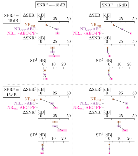
Figure 3: Performance attained by each filter in the NR_ext-AEC-PF by means of the intelligibility-weighted signal-to-echo ratio improvement $\left(\Delta\text{SER\textsuperscript{I}}\right)$, intelligibility-weighted signal-to-noise ratio improvement $\left(\Delta\text{SNR\textsuperscript{I}}\right)$, and intelligibility weighted speech distortion $\left(\text{SD\textsuperscript{I}}\right)$, where a higher $\Delta\text{SER\textsuperscript{I}}$, $\Delta\text{SNR\textsuperscript{I}}$, and an SD^I closer to zero indicates higher performance. The mean performance is represented by the solid dots and the standard deviation by the shading. The performance generally increases with each filter in the cascade.

The NR_ext already improves the SER^I and SNR^I as the NR_ext aims at jointly suppressing the far-end room noise component in the echo and the near-end room noise. This SER^I improvement is larger for echo-dominant than for noise-dominant settings, and vice versa for the SNR^I improvement, since the NR_ext attributes more degrees of freedom towards suppressing the power-dominant interferer.

The AEC further improves the SER^I as the AEC aims at suppressing the echo, and as the excess error in the AEC due to noise perturbations is diminished by prior application of the NR_ext filter. The SNR^I and SD^I remain unaffected by the AEC, as the AEC does not filter the microphone signals, and so does not alter the near-end room noise or the desired speech.

The PF aims at further suppressing the near-end room noise and the echo, such that the PF improves both the SNR^I and SER^I with respect to the NR_ext-AEC. This SNR^I and SER^I improvement comes at the expense of a slightly increased SD^I as both the NR_ext and the PF distort the desired speech.

VI-B Comparison

Fig. 4 compares the performance of the integrated algorithms, as according to Section IV the theoretically equivalent algorithms of Section III differ practically due to non-stationarities and imperfect correlation matrix estimation. To this end, Fig. 4(a) shows the echo cancellation, noise reduction and speech distortion performance separately, which are amalgamated into the instrumental measures of Fig. 4(b). The AEC-NR and NR_ext-AEC-PF generally attain top performance.

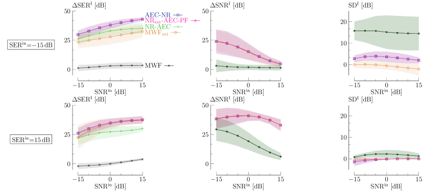
(a) Intelligibility-weighted signal-to-echo ratio improvement $\left(\Delta\text{SER\textsuperscript{I}}\right)$, intelligibility-weighted signal-to-noise ratio improvement $\left(\Delta\text{SNR\textsuperscript{I}}\right)$, and intelligibility weighted speech distortion $\left(\text{SD\textsuperscript{I}}\right)$

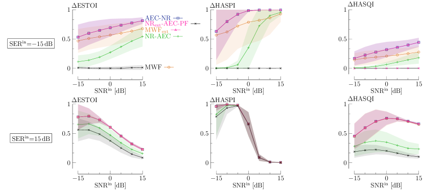
(b) Extended short-time objective intelligibility improvement $\left(\Delta\text{ESTOI}\right)$, hearing-aid speech perception index version 2 improvement $\left(\Delta\text{HASPI}\right)$, and hearing-aid speech quality index version 2 improvement $\left(\Delta\text{HASQI}\right)$

Figure 4: Performance comparison between the integrated algorithms. The mean performance is represented by the solid line and the standard deviation by the shading. Due to non-stationarities and imperfect correlation matrix estimation the theoretically equivalent integrated algorithms differ in their practical performances. To this end, the AEC-NR and NR_ext-AEC-PF generally attain the best performance, characterised by (a) the highest $\Delta$SER^I and $\Delta$SNR^I, and SD^I closest to zero; and (b) the highest $\Delta$ESTOI, $\Delta$HASPI, $\Delta$HASQI.

The MWF attains lower performance than the AEC-NR, as the MWF does not take the loudspeaker information into account. Indeed there are only two microphones, such that the MWF can only completely cancel one interfering source. However, as there are two loudspeakers and one near-end room noise source, there are three interfering sources, such that the MWF lacks the degrees of freedom to cancel these interfering sources. This effect is mostly apparent at $\text{SER\textsuperscript{in}}=$-15\text{\,}\mathrm{dB}$$, as the two echo sources then dominate the one near-end room noise source, leading to low SNR^I, SER^I and instrumental measure improvements, and high SD^I. While the NR in the AEC-NR can also be interpreted as an MWF after preprocessing by an AEC, this NR suffers less from a lack of degrees of freedom as the AEC already partially suppresses the echo, such that the AEC-NR scales with the number of loudspeakers.

The MWF_ext also scales with the number of loudspeakers, in this way increasing the SNR^I, SER^I and instrumental measures and decreasing the SD^I with respect to the MWF. Nevertheless, the MWF_ext SER^I improvement is lower than for the AEC-NR. As described in Section IV, the MWF_ext suffers from loudspeaker and echo non-stationarities, while the AEC in the AEC-NR is less affected, thereby attaining a lower SER^I improvement than the AEC-NR. This effect is primarily visible at $\text{SER\textsuperscript{in}}=$-15\text{\,}\mathrm{dB}$$ as the echo then dominates the noise.

The NR-AEC realises the same decreased SNR^I improvement and high SD^I with respect to the AEC-NR as the MWF. Indeed, the NR of the NR-AEC in its modified form (28) is identical to the MWF. The addition of an AEC after the NR increases the SER^I with respect to the MWF, but as the AEC neither alters the near-end room noise nor the desired speech, the AEC does not alter the SNR^I or the SD^I. Despite the addition of the AEC, the SER^I improvement of the NR-AEC is also inferior to the AEC-NR, as the NR in the NR-AEC already distorts the desired speech, and as the AEC needs to track the NR next to the echo paths. Due to the limited SNR^I improvement and high SD^I, the instrumental measure improvement of the NR-AEC is also limited, as mostly apparent at $\text{SER\textsuperscript{in}}=$-15\text{\,}\mathrm{dB}$$ as the decreased performance of the NR is then mostly apparent.

The NR_ext-AEC-PF also incorporates a filter to suppress the near-end room noise preceding the AEC as for the NR-AEC, namely the NR_ext. However, as opposed to the MWF, the NR_ext next to suppressing the near-end room noise also suppresses the far-end room noise component in the echo, and therefore scales with the number of loudspeakers, resulting in less SD^I and an increased SNR^I with respect to the MWF. The SNR^I improvement of the NR_ext-AEC-PF additionally decreases less quickly with an increasing SNRⁱⁿ than the MWF. In fact, the NR_ext-AEC-PF attains similar performance to the AEC-NR. While, the AEC operates under reduced noise due to the addition of the NR_ext, the AEC, although theoretically independent of the NR^ext, is in practice affected by the NR^ext due to the GEVD and imperfect correlation matrix estimation. This effect is, nevertheless, much more limited than for the NR-AEC due to this theoretical independence between the NR_ext and the AEC as also argued in [18]. Both effects of reduced noise and NR_ext dependence, however, seem to balance each other out, such that the NR_ext-AEC-PF and the AEC-NR achieve a similar performance gain. Alternatively, the NR_ext-AEC-PF can also be interpreted as an AEC-NR preceded by an NR_ext, such that preceding an AEC-NR by an NR_ext does not seem to further increase performance.

In conclusion, the AEC-NR and NR_ext-AEC-PF generally attain top performance as the AEC (theoretically) only needs to model the echo paths, and as the NR operates with reduced echo due to the prior application of the AEC (and NR_ext).

VII Conclusion

In this paper, an integrated approach is proposed for the combined acoustic echo cancellation (AEC) and noise reduction (NR) problem in the general multi-microphone/multi-loudspeaker setup with possible linear dependencies between the loudspeaker and microphone signals. This integrated approach is achieved by selecting a single signal model of either the microphone signal vector or the extended signal vector by stacking microphone and loudspeaker signals, formulating a single mean squared error cost function, and using a common solution strategy. Employing the microphone signal model, an MWF is derived. Similarly, employing the extended signal, an extended MWF (MWF_ext) is derived, for which several theoretically equivalent expressions are found that turn out to be interpretable as specific cascade algorithms. More specifically, the MWF_ext is shown to be theoretically equivalent to the AEC preceding the NR (AEC-NR), the NR preceding the AEC (NR-AEC), and the extended NR (NR_ext) preceding the AEC and a post-filter (PF) (NR_ext-AEC-PF). Under rank-deficiency conditions the MWF_ext is non-unique, such that this theoretical equivalence amounts to the expressions being specific, not necessarily minimum-norm solutions for this MWF_ext.

Nevertheless, although the MWF_ext, AEC-NR, NR-AEC and NR_ext-AEC-PF are theoretically equivalent, their practical performances differ due to non-stationarities and imperfect correlation matrix estimation, leading to the AEC-NR and NR_ext-AEC-PF generally attaining best overall performance.

Integrated Minimum Mean Squared Error Algorithms for Combined Acoustic Echo Cancellation and Noise Reduction: Supplementary Material

This supplementary material relates to the paper Integrated minimum mean squared error algorithms for combined acoustic echo cancellation and noise reduction. For consistency with the main text, all equation, citation, section and page numbers in this supplementary material are compatible with the corresponding numbers in the main text.

In Section VIII, it will be shown that (23) corresponds to a valid generalised inverse in general, and to a pseudo-inverse when $\text{rank}\!\left(\Sigma_{mm}\right)=M$. In Section IX, it will subsequently be shown that (31) is equivalent to (22) if $\text{rank}\!\left(\Sigma_{mm}\right)=M$ as the MWF_ext is then uniquely defined and $R_{\tilde{m}\tilde{m}}^{g,g}$ corresponds to the uniquely-defined pseudoinverse. If $\text{rank}\!\left(\Sigma_{mm}\right)<M$, the MWF_ext (22) is not unique, (31) then still corresponds to one of the solutions of MWF_ext, be it not necessarily the minimum-norm solution. Finally, in Section X, it will be shown that (31) simplifies to (33) when the echo path is linear and the AEC filters are chosen sufficiently long to model this echo path, i.e., $\mathbf{e}=F_{\text{lin}}\mathbf{l}$ and $R_{ee}=R_{ll}F_{\text{lin}}^{H}$.

VIII Proof of (23)

In this section, it is shown that $R_{\tilde{m}\tilde{m}}^{g,g}$ (23) corresponds to a valid generalised inverse of $R_{\tilde{m}\tilde{m}}$ [38] in general, and to a pseudo-inverse of $R_{\tilde{m}\tilde{m}}$ [39] if $\text{rank}\!\left(\Sigma_{mm}\right)=M$.

$R_{\tilde{m}\tilde{m}}$ can be expanded as

$$\begin{IEEEeqnarraybox}[]{rll}R_{\tilde{m}\tilde{m}}=&\begin{bmatrix}\mathbb{I}_{M\times M}&R_{el}R_{ll}^{\dagger}\\ 0_{L\times M}&\mathbb{I}_{L\times L}\end{bmatrix}\cdot\\ &\begin{bmatrix}\Sigma_{mm}&0_{M\times L}\\ 0_{L\times M}&R_{ll}\end{bmatrix}\cdot\\ &\begin{bmatrix}\mathbb{I}_{M\times M}&0_{M\times L}\\ R_{ll}^{\dagger}R_{le}&\mathbb{I}_{L\times L}\end{bmatrix}_{\textstyle\raisebox{2.0pt}{.}}\end{IEEEeqnarraybox}$$ (41)

Similarly, $R_{\tilde{m}\tilde{m}}^{g,g}$ can be expanded as

$$\begin{IEEEeqnarraybox}[]{rll}R_{\tilde{m}\tilde{m}}^{g,g}=&\begin{bmatrix}\mathbb{I}_{M\times M}&0_{M\times L}\\ -R_{ll}^{\dagger}R_{le}&\mathbb{I}_{L\times L}\end{bmatrix}\cdot\\ &\begin{bmatrix}\Sigma_{mm}^{\dagger}&0_{M\times L}\\ 0_{L\times M}&R_{ll}^{\dagger}\end{bmatrix}\cdot\\ &\begin{bmatrix}\mathbb{I}_{M\times M}&-R_{el}R_{ll}^{\dagger}\\ 0_{L\times M}&\mathbb{I}_{L\times L}\end{bmatrix}_{\textstyle\raisebox{2.0pt}{.}}\end{IEEEeqnarraybox}$$ (42)

The condition 1 has to be satisfied for $R_{\tilde{m}\tilde{m}}^{g,g}$ to be a generalised inverse and the conditions 1-4 have to be satisfied for $R_{\tilde{m}\tilde{m}}^{g,g}$ to be a pseudo-inverse.

Condition 1.

$R_{\tilde{m}\tilde{m}}R_{\tilde{m}\tilde{m}}^{g,g}R_{\tilde{m}\tilde{m}}=R_{\tilde{m}\tilde{m}}$

This condition, which is necessary and sufficient for generalised inverses [38], and necessary for pseudo-inverses [39], is satisfied for (23).

Proof.

Using (41) and (42), $R_{\tilde{m}\tilde{m}}R_{\tilde{m}\tilde{m}}^{g,g}R_{\tilde{m}\tilde{m}}$ can be expanded as

$$\begin{IEEEeqnarraybox}[]{rll}R_{\tilde{m}\tilde{m}}R_{\tilde{m}\tilde{m}}^{g,g}R_{\tilde{m}\tilde{m}}=&\begin{bmatrix}\mathbb{I}_{M\times M}&R_{el}R_{ll}^{\dagger}\\ 0_{L\times M}&\mathbb{I}_{L\times L}\end{bmatrix}\begin{bmatrix}\Sigma_{mm}&0_{M\times L}\\ 0_{L\times M}&R_{ll}\end{bmatrix}\cdot\\ &\begin{bmatrix}\mathbb{I}_{M\times M}&0_{M\times L}\\ R_{ll}^{\dagger}R_{le}&\mathbb{I}_{L\times L}\end{bmatrix}\begin{bmatrix}\mathbb{I}_{M\times M}&0_{M\times L}\\ -R_{ll}^{\dagger}R_{le}&\mathbb{I}_{L\times L}\end{bmatrix}\cdot\\ &\begin{bmatrix}\Sigma_{mm}^{\dagger}&0_{M\times L}\\ 0_{L\times M}&R_{ll}^{\dagger}\end{bmatrix}\begin{bmatrix}\mathbb{I}_{M\times M}&-R_{el}R_{ll}^{\dagger}\\ 0_{L\times M}&\mathbb{I}_{L\times L}\end{bmatrix}\cdot\\ &\begin{bmatrix}\mathbb{I}_{M\times M}&R_{el}R_{ll}^{\dagger}\\ 0_{L\times M}&\mathbb{I}_{L\times L}\end{bmatrix}\begin{bmatrix}\Sigma_{mm}&0_{M\times L}\\ 0_{L\times M}&R_{ll}\end{bmatrix}\cdot\\ &\begin{bmatrix}\mathbb{I}_{M\times M}&0_{M\times L}\\ R_{ll}^{\dagger}R_{le}&\mathbb{I}_{L\times L}\end{bmatrix}_{\textstyle\raisebox{2.0pt}{,}}\end{IEEEeqnarraybox}$$ (43)

which can be simplified using $\begin{bmatrix}\mathbb{I}_{M\times M}&0_{M\times L}\\ R_{ll}^{\dagger}R_{le}&\mathbb{I}_{L\times L}\end{bmatrix}\begin{bmatrix}\mathbb{I}_{M\times M}&0_{M\times L}\\ -R_{ll}^{\dagger}R_{le}&\mathbb{I}_{L\times L}\end{bmatrix}=\mathbb{I}_{\left(M+L\right)\times\left(M+L\right)}$ and $\begin{bmatrix}\mathbb{I}_{M\times M}&-R_{el}R_{ll}^{\dagger}\\ 0_{L\times M}&\mathbb{I}_{L\times L}\end{bmatrix}\begin{bmatrix}\mathbb{I}_{M\times M}&R_{el}R_{ll}^{\dagger}\\ 0_{L\times M}&\mathbb{I}_{L\times L}\end{bmatrix}=\mathbb{I}_{\left(M+L\right)\times\left(M+L\right)}$. (43) can then indeed be simplified to

$$\begin{IEEEeqnarraybox}[]{rll}R_{\tilde{m}\tilde{m}}R_{\tilde{m}\tilde{m}}^{g,g}R_{\tilde{m}\tilde{m}}=&\begin{bmatrix}\mathbb{I}_{M\times M}&R_{el}R_{ll}^{\dagger}\\ 0_{L\times M}&\mathbb{I}_{L\times L}\end{bmatrix}\cdot\\ &\begin{bmatrix}\Sigma_{mm}\Sigma_{mm}^{\dagger}\Sigma_{mm}&0_{M\times L}\\ 0_{L\times M}&R_{ll}R_{ll}^{\dagger}R_{ll}\end{bmatrix}\cdot\\ &\begin{bmatrix}\mathbb{I}_{M\times M}&0_{M\times L}\\ R_{ll}^{\dagger}R_{le}&\mathbb{I}_{L\times L}\end{bmatrix}_{\textstyle\raisebox{2.0pt}{.}}\end{IEEEeqnarraybox}$$ (44)

Finally, $\Sigma_{mm}\Sigma_{mm}^{\dagger}\Sigma_{mm}=\Sigma_{mm}$ and $R_{ll}R_{ll}^{\dagger}R_{ll}=R_{ll}$ as per definition of the pseudo-inverse, such that (44) corresponds to

$$R_{\tilde{m}\tilde{m}}R_{\tilde{m}\tilde{m}}^{g,g}R_{\tilde{m}\tilde{m}}=R_{{\tilde{m}\tilde{m}}_{\textstyle\raisebox{2.0pt}{.}}}$$ (45)

∎

Condition 2.

$R_{\tilde{m}\tilde{m}}^{g,g}R_{\tilde{m}\tilde{m}}R_{\tilde{m}\tilde{m}}^{g,g}=R_{\tilde{m}\tilde{m}}^{g,g}$

This condition, which is necessary for pseudo-inverses [39], is satisfied for (23).

Proof.

Using (41) and (42), $R_{\tilde{m}\tilde{m}}^{g,g}R_{\tilde{m}\tilde{m}}R_{\tilde{m}\tilde{m}}^{g,g}$ can be expanded as

$$\begin{IEEEeqnarraybox}[]{rll}R_{\tilde{m}\tilde{m}}^{g,g}R_{\tilde{m}\tilde{m}}R_{\tilde{m}\tilde{m}}^{g,g}=&\begin{bmatrix}\mathbb{I}_{M\times M}&0_{M\times L}\\ -R_{ll}^{\dagger}R_{le}&\mathbb{I}_{L\times L}\end{bmatrix}\begin{bmatrix}\Sigma_{mm}^{\dagger}&0_{M\times L}\\ 0_{L\times M}&R_{ll}^{\dagger}\end{bmatrix}\cdot\\ &\begin{bmatrix}\mathbb{I}_{M\times M}&-R_{el}R_{ll}^{\dagger}\\ 0_{L\times M}&\mathbb{I}_{L\times L}\end{bmatrix}\begin{bmatrix}\mathbb{I}_{M\times M}&R_{el}R_{ll}^{\dagger}\\ 0_{L\times M}&\mathbb{I}_{L\times L}\end{bmatrix}\cdot\\ &\begin{bmatrix}\Sigma_{mm}&0_{M\times L}\\ 0_{L\times M}&R_{ll}\end{bmatrix}\begin{bmatrix}\mathbb{I}_{M\times M}&0_{M\times L}\\ R_{ll}^{\dagger}R_{le}&\mathbb{I}_{L\times L}\end{bmatrix}\cdot\\ &\begin{bmatrix}\mathbb{I}_{M\times M}&0_{M\times L}\\ -R_{ll}^{\dagger}R_{le}&\mathbb{I}_{L\times L}\end{bmatrix}\begin{bmatrix}\Sigma_{mm}^{\dagger}&0_{M\times L}\\ 0_{L\times M}&R_{ll}^{\dagger}\end{bmatrix}\cdot\\ &\begin{bmatrix}\mathbb{I}_{M\times M}&-R_{el}R_{ll}^{\dagger}\\ 0_{L\times M}&\mathbb{I}_{L\times L}\end{bmatrix}_{\textstyle\raisebox{2.0pt}{,}}\end{IEEEeqnarraybox}$$ (46)

which can be simplified using $\begin{bmatrix}\mathbb{I}_{M\times M}&-R_{el}R_{ll}^{\dagger}\\ 0_{L\times M}&\mathbb{I}_{L\times L}\end{bmatrix}\begin{bmatrix}\mathbb{I}_{M\times M}&R_{el}R_{ll}^{\dagger}\\ 0_{L\times M}&\mathbb{I}_{L\times L}\end{bmatrix}=\mathbb{I}_{\left(M+L\right)\times\left(M+L\right)}$ and $\begin{bmatrix}\mathbb{I}_{M\times M}&0_{M\times L}\\ R_{ll}^{\dagger}R_{le}&\mathbb{I}_{L\times L}\end{bmatrix}\begin{bmatrix}\mathbb{I}_{M\times M}&0_{M\times L}\\ -R_{ll}^{\dagger}R_{le}&\mathbb{I}_{L\times L}\end{bmatrix}=\mathbb{I}_{\left(M+L\right)\times\left(M+L\right)}$. (46) can then indeed be simplified to

$$\begin{IEEEeqnarraybox}[]{rll}R_{\tilde{m}\tilde{m}}^{g,g}R_{\tilde{m}\tilde{m}}R_{\tilde{m}\tilde{m}}^{g,g}=&\begin{bmatrix}\mathbb{I}_{M\times M}&0_{M\times L}\\ -R_{ll}^{\dagger}R_{le}&\mathbb{I}_{L\times L}\end{bmatrix}\cdot\\ &\begin{bmatrix}\Sigma_{mm}^{\dagger}\Sigma_{mm}\Sigma_{mm}^{\dagger}&0_{M\times L}\\ 0_{L\times M}&R_{ll}^{\dagger}R_{ll}R_{ll}^{\dagger}\end{bmatrix}\cdot\\ &\begin{bmatrix}\mathbb{I}_{M\times M}&-R_{el}R_{ll}^{\dagger}\\ 0_{L\times M}&\mathbb{I}_{L\times L}\end{bmatrix}_{\textstyle\raisebox{2.0pt}{.}}\end{IEEEeqnarraybox}$$ (47)

Finally, $\Sigma_{mm}^{\dagger}\Sigma_{mm}\Sigma_{mm}^{\dagger}=\Sigma_{mm}^{\dagger}$ and $R_{ll}^{\dagger}R_{ll}R_{ll}^{\dagger}=R_{ll}^{\dagger}$ as per definition of the pseudo-inverse, such that (47) corresponds to

$$R_{\tilde{m}\tilde{m}}^{g,g}R_{\tilde{m}\tilde{m}}R_{\tilde{m}\tilde{m}}^{g,g}=R_{{\tilde{m}\tilde{m}}_{\textstyle\raisebox{2.0pt}{.}}}^{g,g}$$ (48)

∎

Condition 3.

$\left(R_{\tilde{m}\tilde{m}}R_{\tilde{m}\tilde{m}}^{g,g}\right)^{H}=R_{\tilde{m}\tilde{m}}R_{\tilde{m}\tilde{m}}^{g,g}$

This condition, which is necessary for pseudo-inverses [39], is only satisfied for (23) if $\text{rank}\!\left(\Sigma_{mm}\right)=M$.

Proof.

Using (41) and (42), $R_{\tilde{m}\tilde{m}}R_{\tilde{m}\tilde{m}}^{g,g}$ can be expanded as

$$\begin{IEEEeqnarraybox}[]{rll}R_{\tilde{m}\tilde{m}}R_{\tilde{m}\tilde{m}}^{g,g}=&\begin{bmatrix}\mathbb{I}_{M\times M}&R_{el}R_{ll}^{\dagger}\\ 0_{L\times M}&\mathbb{I}_{L\times L}\end{bmatrix}\begin{bmatrix}\Sigma_{mm}&0_{M\times L}\\ 0_{L\times M}&R_{ll}\end{bmatrix}\cdot\\ &\begin{bmatrix}\mathbb{I}_{M\times M}&0_{M\times L}\\ R_{ll}^{\dagger}R_{le}&\mathbb{I}_{L\times L}\end{bmatrix}\begin{bmatrix}\mathbb{I}_{M\times M}&0_{M\times L}\\ -R_{ll}^{\dagger}R_{le}&\mathbb{I}_{L\times L}\end{bmatrix}\cdot\\ &\begin{bmatrix}\Sigma_{mm}^{\dagger}&0_{M\times L}\\ 0_{L\times M}&R_{ll}^{\dagger}\end{bmatrix}\begin{bmatrix}\mathbb{I}_{M\times M}&-R_{el}R_{ll}^{\dagger}\\ 0_{L\times M}&\mathbb{I}_{L\times L}\end{bmatrix}_{\textstyle\raisebox{2.0pt}{,}}\end{IEEEeqnarraybox}$$ (49)

which can be simplified using $\begin{bmatrix}\mathbb{I}_{M\times M}&0_{M\times L}\\ R_{ll}^{\dagger}R_{le}&\mathbb{I}_{L\times L}\end{bmatrix}\begin{bmatrix}\mathbb{I}_{M\times M}&0_{M\times L}\\ -R_{ll}^{\dagger}R_{le}&\mathbb{I}_{L\times L}\end{bmatrix}=\mathbb{I}_{\left(M+L\right)\times\left(M+L\right)}$. (49) can then be simplified to

$$R_{\tilde{m}\tilde{m}}R_{\tilde{m}\tilde{m}}^{g,g}=\begin{bmatrix}\Sigma_{mm}\Sigma_{mm}^{\dagger}&-\Sigma_{mm}\Sigma_{mm}^{\dagger}R_{el}R_{ll}^{\dagger}+R_{el}R_{ll}^{\dagger}\\ 0_{L\times M}&R_{ll}R_{ll}^{\dagger}\end{bmatrix}_{\textstyle\raisebox{2.0pt}{.}}$$ (50)

It is seen that $R_{\tilde{m}\tilde{m}}R_{\tilde{m}\tilde{m}}^{g,g}$ is not Hermitian unless $\text{rank}\!\left(\Sigma_{mm}\right)=M$. Indeed, if $\text{rank}\!\left(\Sigma_{mm}\right)=M$, the pseudo-inverse corresponds to a regular inverse, such that $\Sigma_{mm}\Sigma_{mm}^{\dagger}=\Sigma_{mm}\Sigma_{mm}^{-1}=\mathbb{I}_{M\times M}$ and

$$R_{\tilde{m}\tilde{m}}R_{\tilde{m}\tilde{m}}^{g,g}=\begin{bmatrix}\mathbb{I}_{M\times M}&0_{M\times L}\\ 0_{L\times M}&R_{ll}R_{ll}^{\dagger}\end{bmatrix}_{\textstyle\raisebox{2.0pt}{,}}$$ (51)

which is Hermitian. ∎

Condition 4.

$\left(R_{\tilde{m}\tilde{m}}^{g,g}R_{\tilde{m}\tilde{m}}\right)^{H}=R_{\tilde{m}\tilde{m}}^{g,g}R_{\tilde{m}\tilde{m}}$

This condition, which is necessary for pseudo-inverses [39], is only satisfied for (23) if $\text{rank}\!\left(\Sigma_{mm}\right)=M$.

Proof.

Using (41) and (42), $R_{\tilde{m}\tilde{m}}^{g,g}R_{\tilde{m}\tilde{m}}$ can be expanded as

$$\begin{IEEEeqnarraybox}[]{rll}R_{\tilde{m}\tilde{m}}^{g,g}R_{\tilde{m}\tilde{m}}=&\begin{bmatrix}\mathbb{I}_{M\times M}&0_{M\times L}\\ -R_{ll}^{\dagger}R_{le}&\mathbb{I}_{L\times L}\end{bmatrix}\begin{bmatrix}\Sigma_{mm}^{\dagger}&0_{M\times L}\\ 0_{L\times M}&R_{ll}^{\dagger}\end{bmatrix}\cdot\\ &\begin{bmatrix}\mathbb{I}_{M\times M}&-R_{el}R_{ll}^{\dagger}\\ 0_{L\times M}&\mathbb{I}_{L\times L}\end{bmatrix}\begin{bmatrix}\mathbb{I}_{M\times M}&R_{el}R_{ll}^{\dagger}\\ 0_{L\times M}&\mathbb{I}_{L\times L}\end{bmatrix}\cdot\\ &\begin{bmatrix}\Sigma_{mm}&0_{M\times L}\\ 0_{L\times M}&R_{ll}\end{bmatrix}\begin{bmatrix}\mathbb{I}_{M\times M}&0_{M\times L}\\ R_{ll}^{\dagger}R_{le}&\mathbb{I}_{L\times L}\end{bmatrix}_{\textstyle\raisebox{2.0pt}{,}}\end{IEEEeqnarraybox}$$ (52)

which can be simplified using $\begin{bmatrix}\mathbb{I}_{M\times M}&-R_{el}R_{ll}^{\dagger}\\ 0_{L\times M}&\mathbb{I}_{L\times L}\end{bmatrix}\begin{bmatrix}\mathbb{I}_{M\times M}&R_{el}R_{ll}^{\dagger}\\ 0_{L\times M}&\mathbb{I}_{L\times L}\end{bmatrix}=\mathbb{I}_{\left(M+L\right)\times\left(M+L\right)}$. (52) can then indeed be simplified to

$$R_{\tilde{m}\tilde{m}}^{g,g}R_{\tilde{m}\tilde{m}}=\begin{bmatrix}\Sigma_{mm}^{\dagger}\Sigma_{mm}&0_{M\times L}\\ -R_{ll}^{\dagger}R_{le}\Sigma_{mm}^{\dagger}\Sigma_{mm}+R_{ll}^{\dagger}R_{le}&R_{ll}^{\dagger}R_{ll}\end{bmatrix}_{\textstyle\raisebox{2.0pt}{.}}$$ (53)

It is seen that $R_{\tilde{m}\tilde{m}}^{g,g}R_{\tilde{m}\tilde{m}}$ is not Hermitian unless $\text{rank}\!\left(\Sigma_{mm}\right)=M$. Indeed, if $\text{rank}\!\left(\Sigma_{mm}\right)=M$, the pseudo-inverse corresponds to a regular inverse, such that $\Sigma_{mm}^{\dagger}\Sigma_{mm}=\Sigma_{mm}^{-1}\Sigma_{mm}=\mathbb{I}_{M\times M}$ and

$$R_{\tilde{m}\tilde{m}}^{g,g}R_{\tilde{m}\tilde{m}}=\begin{bmatrix}\mathbb{I}_{M\times M}&0_{M\times L}\\ 0_{L\times M}&R_{ll}^{\dagger}R_{ll}\end{bmatrix}_{\textstyle\raisebox{2.0pt}{,}}$$ (54)

which is Hermitian. ∎

IX Proof of (31)

This section proves that the NR_ext-AEC-PF (31) and MWF_ext (22) are equivalent when choosing $R^{g,g}_{\tilde{m}\tilde{m}}$ as $R^{g}_{\tilde{m}\tilde{m}}$.

The following theorem is used:

Theorem IX.1.

Define the Hermitian positive-semidefinite matrices $A\in\mathbb{C}^{M\times M}$ and $B\in\mathbb{C}^{M\times M}$, where the column space of $A$ is contained within the column space of $B$. Further define $C\in\mathbb{C}^{M\times L}$, whose column space is contained within the column space of $A$. Then,

$$(ABA)^{\dagger}ABC=A^{\dagger}C_{\textstyle\raisebox{2.0pt}{.}}$$ (55)

Proof.

Since the column space of $C$ is contained within $A$, $C$ can be rewritten as $C=AP$ with $P=A^{\dagger}C$, such that $(ABA)^{\dagger}ABC=(ABA)^{\dagger}(ABA)P$. Herein, $(ABA)^{\dagger}(ABA)$ is a projection matrix on the row space of $ABA$. As $A$ and $B$ are Hermitian positive-semidefinite matrices, where the column space of $A$ is contained within the column space of $B$, the row space of $A$ equals the row space of $ABA$. Indeed, joint diagonalisation of $A$ and $B$ using a generalised eigenvalue decomposition (GEVD) with $Q\in\mathbb{C}^{M\times M}$ the generalised eigenvectors, $\Sigma_{A}\in\mathbb{C}^{R_{A}\times R_{A}}$ containing the $R_{A}$ non-zero generalised eigenvalues corresponding to $A$, and $\Sigma_{B}=\begin{bmatrix}\Sigma_{B_{1}}&0_{R_{A}\times(R_{B}-R_{A})}\\ 0_{(R_{B}-R_{A})\times R_{A}}&\Sigma_{B_{2}}\end{bmatrix}\in\mathbb{C}^{R_{B}\times R_{B}}$ containing the $R_{B}$ non-zero generalised eigenvalues corresponding to $B$, yields

$$A =Q\begin{bmatrix}\Sigma_{A}&0_{R_{A}\times(M-R_{A})}\\ 0_{(M-R_{A})\times R_{A}}&0_{(M-R_{A})\times(M-R_{A})}\end{bmatrix}Q^{H}$$ (56a)

$$B =Q\begin{bmatrix}\Sigma_{B}&0_{R_{B}\times(M-R_{B})}\\ 0_{(M-R_{B})\times R_{B}}&0_{(M-R_{B})\times(M-R_{B})}\end{bmatrix}Q^{H}_{\textstyle\raisebox{2.0pt}{.}}$$ (56b)

With $Q=\begin{bmatrix}\smash[b]{\underbrace{Q_{1}}_{R_{A}}}&\smash[b]{\underbrace{Q_{2}}_{(R_{B}-R_{A})}}&\smash[b]{\underbrace{Q_{3}}_{(M-R_{B})}}\end{bmatrix}$, $ABA$ can

subsequently be written as

$$ABA=$$ (57)

$$Q_{1}\left(\begin{bmatrix}\Sigma_{A}&0_{R_{A}\times(R_{B}-R_{A})}\end{bmatrix}\begin{bmatrix}Q_{1}&Q_{2}\end{bmatrix}^{H}\begin{bmatrix}Q_{1}&Q_{2}\end{bmatrix}\Sigma_{B}^{1/2}\right)\cdot$$

$$\left(\Sigma_{B}^{1/2}\begin{bmatrix}Q_{1}&Q_{2}\end{bmatrix}^{H}\begin{bmatrix}Q_{1}&Q_{2}\end{bmatrix}\begin{bmatrix}\Sigma_{A}\\ 0_{(R_{B}-R_{A})\times R_{A}}\end{bmatrix}\right)Q^{H}_{1_{\textstyle\raisebox{2.0pt}{,}}}$$

where both $Q_{1}$ and
$\left(\begin{bmatrix}\Sigma_{A}&0_{R_{A}\times(R_{B}-R_{A})}\end{bmatrix}\begin{bmatrix}Q_{1}&Q_{2}\end{bmatrix}^{H}\begin{bmatrix}Q_{1}&Q_{2}\end{bmatrix}\Sigma_{B}^{1/2}\right)\cdot\\ \left(\Sigma_{B}^{1/2}\begin{bmatrix}Q_{1}&Q_{2}\end{bmatrix}^{H}\begin{bmatrix}Q_{1}&Q_{2}\end{bmatrix}\begin{bmatrix}\Sigma_{A}\\ 0_{(R_{B}-R_{A})\times R_{A}}\end{bmatrix}\right)$ are of rank $R_{A}$, such that the row space of $A$ equals the row space of $ABA$. Consequently, the projection matrix on the row space of $ABA$ corresponds to the projection matrix on the row space of $A$, such that, finally, $(ABA)^{\dagger}(ABA)=A^{\dagger}A$ and $(ABA)^{\dagger}(ABA)P=A^{\dagger}AP=A^{\dagger}C$. ∎

Using the assumption described in Section 3-C5 of the main text that $R_{ll}^{\dagger}R_{le}$ is a solution to the Wiener-Hopf equations $R_{l^{s}l^{s}}W=R_{l^{s}e^{s}}$, i.e., $R_{l^{s}l^{s}}R_{ll}^{\dagger}R_{le}=R_{l^{s}e^{s}}$, $W_{\text{NR\textsubscript{ext}}}=R_{\tilde{m}\tilde{m}}^{g,g}\left(R_{\tilde{s}\tilde{s}}+R_{\tilde{e}^{s}\tilde{e}^{s}}\right)$ corresponds to

$$W_{\text{NR\textsubscript{ext}}}=\begin{bmatrix}W_{\text{NR\textsubscript{ext}}}^{11}&W_{\text{NR\textsubscript{ext}}}^{12}\\ W_{\text{NR\textsubscript{ext}}}^{21}&W_{\text{NR\textsubscript{ext}}}^{22}\end{bmatrix}_{\textstyle\raisebox{2.0pt}{,}}$$ (58)

with

$$W_{\text{NR\textsubscript{ext}}}^{11} =\Sigma_{mm}^{\dagger}\left(R_{ss}+R_{e^{s}e^{s}}-R_{el}R_{ll}^{\dagger}R_{l^{s}e^{s}}\right)$$ (59a)

$$W_{\text{NR\textsubscript{ext}}}^{12} =0_{M\times L}$$ (59b)

$$W_{\text{NR\textsubscript{ext}}}^{21} =-R_{ll}^{\dagger}R_{le}W_{\text{NR\textsubscript{ext}}}^{11}+R_{ll}^{\dagger}R_{l^{s}e^{s}}$$ (59c)

$$W_{\text{NR\textsubscript{ext}}}^{22} =R_{ll}^{\dagger}R_{{l^{s}l^{s}}_{\textstyle\raisebox{2.0pt}{.}}}$$ (59d)

Using (58) and $R_{ll}^{\dagger}R_{ll}R_{ll}^{\dagger}=R_{ll}^{\dagger}$ as per definition of the pseudo-inverse, the correlation matrices $R_{m^{`}m^{`}}$, $R_{l^{`}l^{`}}$, $R_{m^{`}l^{`}}$, $R_{m^{`}l^{`}}R_{l^{`}l^{`}}^{\dagger}R_{l^{`}m^{`}}$, and $R_{l^{`}l^{`}}^{\dagger}R_{l^{`}m^{`}}$ in the NR_ext-AEC-PF (31) can be rewritten in terms of the correlation matrices before applying the NR_ext. Indeed, $R_{m^{`}m^{`}}$ can be rewritten as

$$R_{m^{`}m^{`}} =W_{\text{NR\textsubscript{ext}}}^{11^{H}}R_{mm}W_{\text{NR\textsubscript{ext}}}^{11}+W_{\text{NR\textsubscript{ext}}}^{11^{H}}R_{el}W_{\text{NR\textsubscript{ext}}}^{21}$$

$$+W_{\text{NR\textsubscript{ext}}}^{21^{H}}R_{le}W_{\text{NR\textsubscript{ext}}}^{11}+W_{\text{NR\textsubscript{ext}}}^{21^{H}}R_{ll}W_{\text{NR\textsubscript{ext}}}^{21}$$ (60a)

$$=W_{\text{NR\textsubscript{ext}}}^{11^{H}}\Sigma_{mm}W_{\text{NR\textsubscript{ext}}}^{11}+R_{e^{s}l^{s}}R_{ll}^{\dagger}R_{{l^{s}e^{s}}_{\textstyle\raisebox{2.0pt}{.}}}$$ (60b)

Similarly, $R_{l^{`}l^{`}}$ can be rewritten as

$$R_{l^{`}l^{`}} =W_{\text{NR\textsubscript{ext}}}^{22^{H}}R_{ll}W_{\text{NR\textsubscript{ext}}}^{22}$$ (61a)

$$=R_{l^{s}l^{s}}R_{ll}^{\dagger}R_{{l^{s}l^{s}}_{\textstyle\raisebox{2.0pt}{,}}}$$ (61b)

and $R_{l^{`}m^{`}}$ can be rewritten as

$$R_{l^{`}m^{`}} =W_{\text{NR\textsubscript{ext}}}^{22^{H}}R_{le}W_{\text{NR\textsubscript{ext}}}^{11}+W_{\text{NR\textsubscript{ext}}}^{22^{H}}R_{ll}W_{\text{NR\textsubscript{ext}}}^{21}$$ (62a)

$$=R_{l^{s}l^{s}}R_{ll}^{\dagger}R_{{l^{s}e^{s}}_{\textstyle\raisebox{2.0pt}{.}}}$$ (62b)

Combining (61b) and (62b), $R_{m^{`}l^{`}}R_{l^{`}l^{`}}^{\dagger}R_{l^{`}m^{`}}$ then corresponds to

$$\begin{IEEEeqnarraybox}[]{rll}R_{m^{`}l^{`}}R_{l^{`}l^{`}}^{\dagger}R_{l^{`}m^{`}}=&R_{e^{s}l^{s}}R_{ll}^{\dagger}R_{l^{s}l^{s}}\left(R_{l^{s}l^{s}}R_{ll}^{\dagger}R_{l^{s}l^{s}}\right)^{\dagger}\cdot\\ &R_{l^{s}l^{s}}R_{ll}^{\dagger}R_{{l^{s}e^{s}}_{\textstyle\raisebox{2.0pt}{.}}}\end{IEEEeqnarraybox}$$ (63)

Using the assumption $R_{l^{s}l^{s}}R_{ll}^{\dagger}R_{le}=R_{l^{s}e^{s}}$, (63) can further be expanded as

$$\begin{IEEEeqnarraybox}[]{rll}&R_{m^{`}l^{`}}R_{l^{`}l^{`}}^{\dagger}R_{l^{`}m^{`}}=R_{el}R_{ll}^{\dagger}\left(R_{l^{s}l^{s}}R_{ll}^{\dagger}R_{l^{s}l^{s}}\right)\cdot\\ &\qquad\left(R_{l^{s}l^{s}}R_{ll}^{\dagger}R_{l^{s}l^{s}}\right)^{\dagger}\left(R_{l^{s}l^{s}}R_{ll}^{\dagger}R_{l^{s}l^{s}}\right)R_{ll}^{\dagger}R_{{le}_{\textstyle\raisebox{2.0pt}{,}}}\end{IEEEeqnarraybox}$$ (64)

where $\left(R_{l^{s}l^{s}}R_{ll}^{\dagger}R_{l^{s}l^{s}}\right)\left(R_{l^{s}l^{s}}R_{ll}^{\dagger}R_{l^{s}l^{s}}\right)^{\dagger}\left(R_{l^{s}l^{s}}R_{ll}^{\dagger}R_{l^{s}l^{s}}\right)=\left(R_{l^{s}l^{s}}R_{ll}^{\dagger}R_{l^{s}l^{s}}\right)$ as per definition of the pseudo-inverse. Again using the assumption $R_{l^{s}l^{s}}R_{ll}^{\dagger}R_{le}=R_{l^{s}e^{s}}$, (64) can subsequently be rewritten as

$$R_{m^{`}l^{`}}R_{l^{`}l^{`}}^{\dagger}R_{l^{`}m^{`}}=R_{e^{s}l^{s}}R_{ll}^{\dagger}R_{{l^{s}e^{s}}_{\textstyle\raisebox{2.0pt}{.}}}$$ (65)

$R_{l^{`}l^{`}}^{\dagger}R_{l^{`}m^{`}}$ similarly corresponds to

$$R_{l^{`}l^{`}}^{\dagger}R_{l^{`}m^{`}}=\left(R_{l^{s}l^{s}}R_{ll}^{\dagger}R_{l^{s}l^{s}}\right)^{\dagger}R_{l^{s}l^{s}}R_{ll}^{\dagger}R_{{l^{s}e^{s}}_{\textstyle\raisebox{2.0pt}{.}}}$$ (66)

As $R_{l^{s}l^{s}}$ and $R_{ll}$ are Hermitian positive-semidefinite matrices, the column space of $R_{l^{s}l^{s}}$ is contained within the column space of $R_{ll}$, and the column space of $R_{l^{s}e^{s}}$ is contained within the column space of $R_{l^{s}l^{s}}$, Theorem IX.1 can thus be applied to (66), resulting in

$$R_{l^{`}l^{`}}^{\dagger}R_{l^{`}m^{`}}=R_{l^{s}l^{s}}^{\dagger}R_{{l^{s}e^{s}}_{\textstyle\raisebox{2.0pt}{.}}}$$ (67)

Using these rewritten correlation matrices, it can be shown that
$\left(R_{\tilde{s}\tilde{s}}+R_{\tilde{e}^{s}\tilde{e}^{s}}\right)\begin{bmatrix}\Sigma_{m^{`}m^{`}}^{\dagger}R_{s^{`}s}&0_{M\times L}\\ -R_{l^{`}l^{`}}^{\dagger}R_{l^{`}m^{`}}\Sigma_{m^{`}m^{`}}^{\dagger}R_{s^{`}s}&0_{L\times L}\end{bmatrix}=R_{\tilde{s}\tilde{s}}$, as this expression can be expanded using (67) as

$$\begin{IEEEeqnarraybox}[]{rll}&\left(R_{\tilde{s}\tilde{s}}+R_{\tilde{e}^{s}\tilde{e}^{s}}\right)\begin{bmatrix}\Sigma_{m^{`}m^{`}}^{\dagger}R_{s^{`}s}&0_{M\times L}\\ -R_{l^{`}l^{`}}^{\dagger}R_{l^{`}m^{`}}\Sigma_{m^{`}m^{`}}^{\dagger}R_{s^{`}s}&0_{L\times L}\end{bmatrix}=\\ &\begin{bmatrix}\left(R_{ss}+R_{e^{s}e^{s}}-R_{e^{s}l^{s}}R_{l^{s}l^{s}}^{\dagger}R_{l^{s}e^{s}}\right)\Sigma_{m^{`}m^{`}}^{\dagger}R_{s^{`}s}&0_{M\times L}\\ \left(R_{l^{s}e^{s}}-R_{l^{s}l^{s}}R_{l^{s}l^{s}}^{\dagger}R_{l^{s}e^{s}}\right)\Sigma_{m^{`}m^{`}}^{\dagger}R_{s^{`}s}&0_{L\times L}\end{bmatrix}_{\textstyle\raisebox{2.0pt}{.}}\end{IEEEeqnarraybox}$$ (68)

Here, $R_{l^{s}e^{s}}-R_{l^{s}l^{s}}R_{l^{s}l^{s}}^{\dagger}R_{l^{s}e^{s}}=0_{L\times M}$ as $R_{l^{s}l^{s}}R_{l^{s}l^{s}}^{\dagger}$ is a projection on the column space of $R_{l^{s}l^{s}}$ and the column space of $R_{l^{s}e^{s}}$ is contained within the column space of $R_{l^{s}l^{s}}$. Furthermore, using (60b) and (65) $\left(R_{ss}+R_{e^{s}e^{s}}-R_{e^{s}l^{s}}R_{l^{s}l^{s}}^{\dagger}R_{l^{s}e^{s}}\right)\Sigma_{m^{`}m^{`}}^{\dagger}R_{s^{`}s}$ corresponds to

$$\begin{IEEEeqnarraybox}[]{rll}&\left(R_{ss}+R_{e^{s}e^{s}}-R_{e^{s}l^{s}}R_{l^{s}l^{s}}^{\dagger}R_{l^{s}e^{s}}\right)\Sigma_{m^{`}m^{`}}^{\dagger}R_{s^{`}s}=\\ &\left(R_{ss}+R_{e^{s}e^{s}}-R_{e^{s}l^{s}}R_{l^{s}l^{s}}^{\dagger}R_{l^{s}e^{s}}\right)\left(W^{11^{H}}_{\text{NR\textsubscript{ext}}}\Sigma_{mm}W^{11}_{\text{NR\textsubscript{ext}}}\right)^{\dagger}\cdot\\ &W^{11^{H}}_{\text{NR\textsubscript{ext}}}R_{{ss}_{\textstyle\raisebox{2.0pt}{,}}}\end{IEEEeqnarraybox}$$ (69)

which can be further expanded using (58) and $\Sigma_{mm}^{\dagger}\Sigma_{mm}\Sigma_{mm}^{\dagger}=\Sigma_{mm}^{\dagger}$ as per definition of the pseudo-inverse as

$$\begin{IEEEeqnarraybox}[]{rll}&\left(R_{ss}+R_{e^{s}e^{s}}-R_{e^{s}l^{s}}R_{l^{s}l^{s}}^{\dagger}R_{l^{s}e^{s}}\right)\Sigma_{m^{`}m^{`}}^{\dagger}R_{s^{`}s}=\\ &\left(R_{ss}+R_{e^{s}e^{s}}-R_{e^{s}l^{s}}R_{l^{s}l^{s}}^{\dagger}R_{l^{s}e^{s}}\right)\cdot\\ &\biggl{[}\left(R_{ss}+R_{e^{s}e^{s}}-R_{el}R_{ll}^{\dagger}R_{l^{s}e^{s}}\right)\Sigma_{mm}^{\dagger}\cdot\\ &\left(R_{ss}+R_{e^{s}e^{s}}-R_{el}R_{ll}^{\dagger}R_{l^{s}e^{s}}\right)\biggr{]}^{\dagger}\cdot\\ &\left(R_{ss}+R_{e^{s}e^{s}}-R_{el}R_{ll}^{\dagger}R_{l^{s}e^{s}}\right)\Sigma_{mm}^{\dagger}R_{ss_{\textstyle\raisebox{2.0pt}{.}}}\end{IEEEeqnarraybox}$$ (70)

Further, $R_{el}R_{ll}^{\dagger}R_{l^{s}e^{s}}=R_{e^{s}l^{s}}R_{l^{s}l^{s}}^{\dagger}R_{l^{s}e^{s}}$ due to the assumption $R_{l^{s}l^{s}}R_{ll}^{\dagger}R_{le}=R_{l^{s}e^{s}}$ and due to $R_{l^{s}l^{s}}R_{l^{s}l^{s}}^{\dagger}R_{l^{s}e^{s}}=R_{l^{s}e^{s}}$, such that $R_{ss}$ + $R_{e^{s}e^{s}}-R_{el}R_{ll}^{\dagger}R_{l^{s}e^{s}}=R_{ss}$ + $R_{e^{s}e^{s}}-R_{e^{s}l^{s}}R_{l^{s}l^{s}}^{\dagger}R_{l^{s}e^{s}}$ can be seen to be a Hermitian matrix. Thus, since $R_{ss}+R_{e^{s}e^{s}}-R_{e^{s}l^{s}}R_{l^{s}l^{s}}^{\dagger}R_{l^{s}e^{s}}$ and $\Sigma_{mm}$ are Hermitian positive-semidefinite matrices, and since the column space of $R_{ss}$ + $R_{e^{s}e^{s}}-R_{e^{s}l^{s}}R_{l^{s}l^{s}}^{\dagger}R_{l^{s}e^{s}}$ is contained within the column space of $\Sigma_{mm}$, as per Theorem IX.1, (70) corresponds to

$$\begin{IEEEeqnarraybox}[]{rll}&\left(R_{ss}+R_{e^{s}e^{s}}-R_{e^{s}l^{s}}R_{l^{s}l^{s}}^{\dagger}R_{l^{s}e^{s}}\right)\Sigma_{m^{`}m^{`}}^{\dagger}R_{s^{`}s}=\\ &\left(R_{ss}+R_{e^{s}e^{s}}-R_{e^{s}l^{s}}R_{l^{s}l^{s}}^{\dagger}R_{l^{s}e^{s}}\right)\cdot\\ &\left(R_{ss}+R_{e^{s}e^{s}}-R_{e^{s}l^{s}}R_{l^{s}l^{s}}^{\dagger}R_{l^{s}e^{s}}\right)^{\dagger}R_{ss_{\textstyle\raisebox{2.0pt}{.}}}\end{IEEEeqnarraybox}$$ (71)

Additionally, since the column space of $R_{ss}$ is contained within the column space of $R_{ss}+R_{e^{s}e^{s}}-R_{e^{s}l^{s}}R_{l^{s}l^{s}}^{\dagger}R_{l^{s}e^{s}}$, (71) corresponds to

$$\begin{IEEEeqnarraybox}[]{rll}&\left(R_{ss}+R_{e^{s}e^{s}}-R_{e^{s}l^{s}}R_{l^{s}l^{s}}^{\dagger}R_{l^{s}e^{s}}\right)\Sigma_{m^{`}m^{`}}^{\dagger}R_{s^{`}s}=R_{ss_{\textstyle\raisebox{2.0pt}{.}}}\end{IEEEeqnarraybox}$$ (72)

Finally, using (72), the MWF_ext (22) is obtained, such that the NR_ext-AEC-PF (31) is shown to correspond to the MWF_ext (22) when $R_{\tilde{m}\tilde{m}}^{g,g}$ is selected for $R_{\tilde{m}\tilde{m}}^{g}$, i.e.,

$$\begin{IEEEeqnarraybox}[]{rll}&R_{\tilde{m}\tilde{m}}^{g,g}\left(R_{\tilde{s}\tilde{s}}+R_{\tilde{e}^{s}\tilde{e}^{s}}\right)\begin{bmatrix}\mathbb{I}_{M\times M}&0_{M\times L}\\ -R_{l^{`}l^{`}}^{\dagger}R_{l^{`}m^{`}}&0_{L\times L}\end{bmatrix}\begin{bmatrix}\Sigma_{m^{`}m^{`}}^{\dagger}R_{s^{`}s}\\ {0}_{L\times M}\end{bmatrix}{\mathbf{t}}_{r}\\ &=R_{\tilde{m}\tilde{m}}^{g,g}R_{\tilde{s}\tilde{s}}\tilde{\mathbf{t}}_{r_{\textstyle\raisebox{2.0pt}{.}}}\end{IEEEeqnarraybox}$$ (73)

$$\IEEEQEDhereeqn$$

X Proof of (33)

This section proves that (33) is obtained from the general NR_ext-AEC-PF (31) expression if the echo path is linear and the filters are sufficiently long to model this echo path, i.e., $\mathbf{e}=F_{\text{lin}}\mathbf{l}$ and $R_{le}=R_{ll}F_{\text{lin}}^{H}$.

With $\mathbf{e}=F_{\text{lin}}\mathbf{l}$, $R_{le}=R_{ll}F_{\text{lin}}^{H}$ and $R_{l^{s}e^{s}}=R_{l^{s}l^{s}}F_{\text{lin}}^{H}$, the $W_{\text{NR\textsubscript{ext}}}$ filter (58) simplifies to

$$\begin{IEEEeqnarraybox}[]{rll}&W_{\text{NR\textsubscript{ext}}}=\\ &\qquad\begin{bmatrix}\left(R_{ss}+R_{nn}\right)^{\dagger}R_{ss}&0_{M\times L}\\ -R_{ll}^{\dagger}R_{le}\left(R_{ss}+R_{nn}\right)^{\dagger}R_{ss}+R_{ll}^{\dagger}R_{l^{s}e^{s}}&R_{ll}^{\dagger}R_{l^{s}l^{s}}\end{bmatrix}_{\textstyle\raisebox{2.0pt}{.}}\end{IEEEeqnarraybox}$$ (74)

In the AEC, $R_{l^{`}l^{`}}^{\dagger}R_{l^{`}m^{`}}$ corresponds to $R_{l^{s}l^{s}}^{\dagger}R_{l^{s}e^{s}}$ (cfr. Supplementary material Section IX). Finally, in the PF, $\Sigma_{m^{`}m^{`}}^{\dagger}R_{s^{`}s}$ corresponds to

$$\begin{IEEEeqnarraybox}[]{rll}&\Sigma_{m^{`}m^{`}}^{\dagger}R_{s^{`}s}=\\ &\qquad\left(R_{ss}\left(R_{ss}+R_{nn}\right)^{\dagger}R_{ss}\right)^{\dagger}R_{ss}\left(R_{ss}+R_{nn}\right)^{\dagger}R_{{ss}_{\textstyle\raisebox{2.0pt}{,}}}\end{IEEEeqnarraybox}$$ (75)

which can be further simplified using Theorem IX.1 as $R_{ss}+R_{nn}$ and $R_{ss}$ are Hermitian positive-semidefinite matrices, and the column space of $R_{ss}$ is contained within the column space of $R_{ss}+R_{nn}$. Thus, $\Sigma_{m^{`}m^{`}}^{\dagger}R_{s^{`}s}$ corresponds to

$$\Sigma_{m^{`}m^{`}}^{\dagger}R_{s^{`}s}=R_{ss}^{\dagger}R_{{ss}_{\textstyle\raisebox{2.0pt}{.}}}$$ (76)

Consequently, the general NR_ext-AEC-PF (31) expression can be simplified to $\tilde{\mathbf{w}}_{\text{int,lin}}$ with

$$\begin{IEEEeqnarraybox}[]{rll}\tilde{\mathbf{w}}_{\text{int,lin}}&{=}\underbrace{\begin{bmatrix}\left(R_{ss}+R_{nn}\right)^{\dagger}R_{ss}&0_{M\times L}\\ -R_{ll}^{\dagger}R_{le}\left(R_{ss}+R_{nn}\right)^{\dagger}R_{ss}+R_{ll}^{\dagger}R_{l^{s}e^{s}}&R_{ll}^{\dagger}R_{l^{s}l^{s}}\end{bmatrix}}_{\text{NR\textsubscript{ext}}}\cdot\\ &\underbrace{\begin{bmatrix}\mathbb{I}_{M\times M}&0_{M\times L}\\ -R_{l^{s}l^{s}}^{\dagger}R_{l^{s}e^{s}}&0_{L\times L}\end{bmatrix}}_{\text{AEC}}\underbrace{\begin{bmatrix}R_{ss}^{\dagger}R_{ss}\\ {0}_{L\times M}\end{bmatrix}}_{\text{PF}}{\mathbf{t}_{r_{\textstyle\raisebox{2.0pt}{.}}}}\end{IEEEeqnarraybox}$$ (77)

Finally, as $R_{l^{s}e^{s}}=R_{l^{s}l^{s}}R_{l^{s}l^{s}}^{\dagger}R_{l^{s}e^{s}}$ (cfr. Supplementary material Section IX) and $R_{ss}R_{ss}^{\dagger}R_{ss}=R_{ss}$ as per definition of the pseudo-inverse, (33) is obtained

$$\tilde{\mathbf{w}}_{\text{int}}{=}{\underbrace{R_{\tilde{m}\tilde{m}}^{g,g}\left(R_{\tilde{s}\tilde{s}}+R_{\tilde{e}^{s}\tilde{e}^{s}}\right)}_{\text{NR\textsubscript{ext}}}\underbrace{\begin{bmatrix}\mathbb{I}_{M\times M}\\ -R_{l^{s}l^{s}}^{\dagger}R_{l^{s}l^{s}}F_{\text{lin}}^{H}\end{bmatrix}}_{\text{AEC}}}{\mathbf{t}}_{r_{\textstyle\raisebox{2.0pt}{.}}}$$ (78)

$$\IEEEQEDhereeqn$$

References

- [1] E. Hänsler and G. Schmidt, Topics in acoustic echo and noise control. Berlin, Heidelberg: Springer-Verlag, 2006.
- [2] N. Fleischhacker, “The tikzpeople package,” 2017. [Online]. Available: https://ctan.org/pkg/tikzpeople
- [3] F. Yang, M. Wu, and J. Yang, “Stereophonic acoustic echo suppression based on Wiener filter in the short-time Fourier transform domain,” IEEE Signal Process. Lett., vol. 19, no. 4, pp. 227–230, Apr. 2012.
- [4] C. Zhang, J. Liu, H. Li, and X. Zhang, “Neural multi-channel and multi-microphone acoustic echo cancellation,” IEEE/ACM Trans. Audio, Speech, Language Process., vol. 31, pp. 1–12, 2023.
- [5] A. Fazel, M. El-Khamy, and J. Lee, “CAD-AEC: Context-aware deep acoustic echo cancellation,” in Proc. 2020 IEEE Int. Conf. Acoust., Speech, Signal Process. (ICASSP), Barcelona, Spain, May 2020, pp. 6919–6923.
- [6] J. Benesty, J. Chen, Y. A. Huang, and S. Doclo, “Study of the Wiener filter for noise reduction,” in Speech enhancement, ser. Signals and Commun. Technol., J. Benesty, S. Makino, and J. Chen, Eds. Berlin, Heidelberg: Springer, 2005, pp. 9–41.
- [7] S. Doclo, W. Kellermann, S. Makino, and S. E. Nordholm, “Multichannel signal enhancement algorithms for assisted listening devices: Exploiting spatial diversity using multiple microphones,” IEEE Signal Process. Mag., vol. 32, no. 2, pp. 18–30, Mar. 2015.
- [8] S. Gannot, “Speech processing utilizing the Kalman filter,” IEEE Instrum. Meas. Mag., vol. 15, no. 3, pp. 10–14, Jun. 2012.
- [9] R. C. Hendriks, T. Gerkmann, and J. Jensen, DFT-domain based single-microphone noise reduction for speech enhancement: A survey of the state-of-the-art. Switzerland: Springer, 2013.
- [10] W. Jiang, C. Sun, F. Chen, Y. Leng, and Q. Guo, “A novel skip connection mechanism based on channel-wise cross transformer for speech enhancement,” Multimedia Tools and Appl., vol. 83, no. 12, Sep. 2023.
- [11] Z. Zhang, Y. Xu, M. Yu, S.-X. Zhang, L. Chen, and D. Yu, “ADL-MVDR: All deep learning MVDR beamformer for target speech separation,” in Proc. 2021 IEEE Int. Conf. Acoust., Speech, Signal Proces. (ICASSP), Toronto, ON, Canada, Jun. 2021, pp. 6089–6093.
- [12] S. Gustafsson, R. Martin, and P. Vary, “Combined acoustic echo control and noise reduction for hands-free telephony,” Signal Process., vol. 64, no. 1, pp. 21–32, Jan. 1998.
- [13] A. Cohen, A. Barnov, S. Markovich-Golan, and P. Kroon, “Joint beamforming and echo cancellation combining QRD based multichannel AEC and MVDR for reducing noise and non-linear echo,” in Proc. 26th European Signal Process. Conf. (EUSIPCO), Rome, Italy, Sep. 2018, pp. 6–10.
- [14] M. Luis Valero and E. A. P. Habets, “Low-complexity multi-microphone acoustic echo control in the short-time Fourier transform domain,” IEEE/ACM Trans. Audio, Speech, Language Process., vol. 27, no. 3, pp. 595–609, Mar. 2019.
- [15] R. Martin, S. Gustafsson, and M. Moser, “Acoustic echo cancellation for microphone arrays using switched coefficient vectors,” in Proc. 1997 Int. Workshop Acoustic Echo Noise Control (IWAENC), London, United Kingdom, 1997, pp. I–85.
- [16] S. Doclo, M. Moonen, and E. de Clippel, “Combined acoustic echo and noise reduction using GSVD-based optimal filtering,” in Proc. 2000 IEEE Int. Conf. Acoust., Speech, Signal Process. (ICASSP), Istanbul, Turkey, Jun. 2000, pp. II1061–II1064 vol.2.
- [17] M. Schrammen, A. Bohlender, S. Kühl, and P. Jax, “Change prediction for low complexity combined beamforming and acoustic echo cancellation,” in Proc. 27th European Signal Process. Conf. (EUSIPCO), A Coruna, Spain, Sep. 2019, pp. 1–5.
- [18] A. Roebben, T. van Waterschoot, and M. Moonen, “Cascaded noise reduction and acoustic echo cancellation based on an extended noise reduction,” in Proc. 32th European Signal Process. Conf. (EUSIPCO), Lyon, France, 2024.
- [19] W. Jeannes, P. Scalart, G. Faucon, and C. Beaugeant, “Combined noise and echo reduction in hands-free systems: A survey,” IEEE Trans. Speech Audio Process., vol. 9, no. 8, pp. 808–820, Nov. 2001.
- [20] W. Herbordt, H. Buchner, and W. Kellermann, “An acoustic human-machine front-end for multimedia applications,” EURASIP J. Advances Signal Process., vol. 2003, no. 1, pp. 1–11, Dec. 2003.
- [21] T. Burton and R. Goubran, “A new structure for combining echo cancellation and beamforming in changing acoustical environments,” in Proc. 2007 IEEE Int. Conf. Acoust., Speech, Signal Process. (ICASSP), Honolulu, HI, USA, Apr. 2007, pp. I–77–I–80.
- [22] G. Reuven, S. Gannot, and I. Cohen, “Joint acoustic echo cancellation and transfer function GSC in the frequency domain,” in Proc. 23rd IEEE Conv. Elect. Electronics Engineers Israel, Tel-Aviv, Israel, Sep. 2004, pp. 412–415.
- [23] S. Gustafsson, P. Jax, A. Kamphausen, and P. Vary, “A postfilter for echo and noise reduction avoiding the problem of musical tones,” in Proc. 1999 IEEE Int. Conf. Acoust., Speech, Signal Process. (ICASSP), Phoenix, AZ, USA, Mar. 1999, pp. 873–876 vol.2.
- [24] W. Herbordt, W. Kellermann, and S. Nakamura, “Joint optimization of LCMV beamforming and acoustic echo cancellation,” in Proc. 12th European Signal Process. Conf. (EUSIPCO), Vienna, Austria, Sep. 2004, pp. 2003–2006.
- [25] M. H. Maruo, J. C. M. Bermudez, and L. S. Resende, “On the optimal solutions of beamformer assisted acoustic echo cancellers,” in Proc. 2011 IEEE Statistical Signal Process. Workshop (SSP), Nice, Jun. 2011, pp. 641–644.
- [26] K. Nathwani, “Joint acoustic echo and noise cancellation using spectral domain Kalman filtering in double-talk scenario,” in Proc. 2018 Int. Workshop Acoustic Echo Noise Control (IWAENC), Tokyo, Japan, Sep. 2018, pp. 1–330.
- [27] E. A. P. Habets, I. Cohen, and S. Gannot, “MMSE log-spectral amplitude estimator for multiple interferences,” in Proc. 2006 Int. Workshop Acoustic Echo Noise Control (IWAENC), Paris, France, 2006.
- [28] Y.-S. Park and J.-H. Chang, “Integrated acoustic echo and background noise suppression technique based on soft decision,” EURASIP J. Advances in Signal Process., vol. 2012, no. 1, p. 11, Jan. 2012.
- [29] E. P. Jayakumar, P. V. M. Shifas, and P. S. Sathidevi, “Integrated acoustic echo and noise suppression in modulation domain,” Int. J. Speech Technol., vol. 19, no. 3, pp. 611–621, Sep. 2016.
- [30] E. Shachar, I. Cohen, and B. Berdugo, “Acoustic echo cancellation with the normalized sign-error least mean squares algorithm and deep residual echo suppression,” Algorithms, vol. 16, no. 3, p. 137, Mar. 2023.
- [31] H. Zhang, K. Tan, and D. Wang, “Deep learning for joint acoustic echo and noise cancellation with nonlinear distortions,” in Proc. Interspeech 2019, Graz, Austria, Jun. 2019, pp. 15–19.
- [32] S. Doclo, “Multi-microphone noise reduction and dereverberation techniques for speech applications,” Ph.D. dissertation, KU Leuven, Leuven, Belgium, 2003.
- [33] G. Rombouts and M. Moonen, “An integrated approach to acoustic noise and echo cancellation,” Signal Process., vol. 85, no. 4, pp. 849–871, Apr. 2005.
- [34] S. Ruiz, T. van Waterschoot, and M. Moonen, “Distributed combined acoustic echo cancellation and noise reduction in wireless acoustic sensor and actuator networks,” IEEE/ACM Trans. Audio, Speech, Language Proc., vol. 30, pp. 534–547, 2022.
- [35] ——, “Cascade Multi-Channel Noise Reduction and Acoustic Feedback Cancellation,” in Proc. 2022 IEEE Int. Conf. Acoust., Speech and Signal Process. (ICASSP), Singapore, Singapore, May 2022, pp. 676–680.
- [36] A. Roebben, “Github repository: Integrated minimum mean square error algorithms for combined acoustic echo cancellation and noise reduction,” https://github.com/Arnout-Roebben/Integrated_AEC_NR, 2024.
- [37] J. Benesty, T. Gänsler, D. R. Morgan, M. M. Sondhi, and S. L. Gay, Advances in network and acoustic echo cancellation, ser. Digital Signal Processing, A. Lacroix and A. Venetsanopoulos, Eds. Berlin, Heidelberg: Springer Berlin Heidelberg, 2001.
- [38] M. James, “The generalised inverse,” The Math. Gazette, vol. 62, no. 420, pp. 109–114, 1978.
- [39] R. Penrose, “A generalized inverse for matrices,” Math. Proc. Cambridge Philos. Soc., vol. 51, no. 3, pp. 406–413, Jul. 1955.
- [40] R. Serizel, M. Moonen, B. Van Dijk, and J. Wouters, “Low-rank approximation based multichannel Wiener filter algorithms for noise reduction with application in cochlear implants,” IEEE/ACM Trans. Audio, Speech, Language Process., vol. 22, no. 4, pp. 785–799, Apr. 2014.
- [41] S. Shimauchi and S. Makino, “Stereo projection echo canceller with true echo path estimation,” in Proc. 1995 IEEE Int. Conf. Acoust., Speech, Signal Process. (ICASSP), vol. 5, May 1995, pp. 3059–3062 vol.5.
- [42] Z. Bai, J. Demmel, J. Dongarra, A. Ruhe, and H. van der Vorst, Eds., Templates for the solution of algebraic eigenvalue problems. Philadelphia: SIAM, 2000.
- [43] E. De Sena, N. Antonello, M. Moonen, and T. van Waterschoot, “On the modeling of rectangular geometries in room acoustic simulations,” IEEE/ACM Trans. Audio, Speech, Language Process., vol. 23, no. 4, pp. 774–786, Apr. 2015.
- [44] M. Nilsson, S. D. Ewert, and J. A. Sullivan, “Development of the Hearing In Noise Test for the measurement of speech reception thresholds in quiet and in noise,” Acoust. Soc. Amer., vol. 95, no. 2, pp. 1085–1099, Feb. 1994.
- [45] Auditec, “Auditory Tests (Revised), Compact Disc, Auditec,” St. Louis, MO, 1997.
- [46] J. E. Greenberg, P. M. Peterson, and P. M. Zurek, “Intelligibility-weighted measures of speech-to-interference ratio and speech system performance,” Acoust. Soc. Amer., vol. 94, no. 5, pp. 3009–3010, Nov. 1993.
- [47] A. Spriet, “Adaptive filtering techniques for noise reduction and acoustic feedback cancellation in hearing aids,” Ph.D. dissertation, KU Leuven, Leuven, Belgium, 2004.
- [48] Acoustical Society of America, “ANSI S3.5-1997 American National Standard Methods for calculation of the speech intelligibility index,” 1997.
- [49] J. Jensen and C. H. Taal, “An algorithm for predicting the intelligibility of speech masked by modulated noise maskers,” IEEE/ACM Trans. Audio, Speech, Language Process., vol. 24, no. 11, pp. 2009–2022, Nov. 2016.
- [50] J. M. Kates and K. H. Arehart, “The hearing-aid speech perception index (HASPI) Version 2,” Speech Communication, vol. 131, pp. 35–46, Jul. 2021.
- [51] J. Kates and K. Arehart, “The hearing-aid speech quality index (HASQI) Version 2,” J. Audio Eng. Soc., vol. 62, no. 3, pp. 99–117, Mar. 2014.