On Extrapolation of Treatment Effects in Multiple-Cutoff Regression Discontinuity Designs

Abstract

Regression discontinuity (RD) designs typically identify the treatment effect at a single cutoff point. But when and how can we learn about treatment effects away from the cutoff? This paper addresses this question within a multiple-cutoff RD framework. We begin by examining the plausibility of the constant bias assumption proposed by Cattaneo, Keele, Titiunik, and Vazquez-Bare (2021) through the lens of rational decision-making behavior, which suggests that a kind of similarity between groups and whether individuals can influence the running variable are important factors. We then introduce an alternative set of assumptions and propose a broadly applicable partial identification strategy. The potential applicability and usefulness of the proposed bounds are illustrated through two empirical examples.

1 Introduction

Regression discontinuity (RD) designs are among the most credible quasi-experimental approaches for identifying causal effects (Brodeur et al.,, 2020). In the RD framework, treatment status changes discontinuously at a known threshold, allowing for the identification of the treatment effect at the cutoff, provided a mild smoothness assumption holds (Hahn et al.,, 2001). This exogenous jump provides RD designs with strong internal validity; however, their external validity often remains uncertain (Abadie and Cattaneo,, 2018). This is a primary limitation of RD designs, as the treatment effect estimated at the single cutoff is not necessarily the only parameter of interest, and a researcher is often also interested in the treatment effect away from the cutoff to guarantee a certain external validity of the local estimate (Dong and Lewbel,, 2015; Cerulli et al.,, 2017). Furthermore, in some cases, a policymaker is interested in the treatment effect at specific points other than the current cutoff point. Standard RD designs, however, provide limited information to answer these questions.

An additional source of information is required to address the issue of weaker external validity in RD designs and learn about the effect beyond the cutoff point. A promising approach is to leverage the existence of multiple cutoffs, a scenario commonly encountered in empirical research. For instance, it is often the case that the eligibility threshold for a scholarship varies based on a student’s background, race, or cohort. Although such multiple cutoffs have often been normalized, Cattaneo et al., (2021) recently proposed a novel alternative strategy to identify the treatment effect away from the cutoff point by effectively utilizing these multiple cutoffs. Their identification strategy is as follows: Let $\mu_{0,l}(x)$ and $\mu_{1,l}(x)$ represent the conditional expectation functions under control and treatment status and let $l$ be the cutoff point (Figure 1). We typically identify and estimate $\mu_{1,l}(l)-\mu_{0,l}(l)$. A fundamental challenge in extrapolation is that an economist can observe $\mu_{1,l}(x)$ but cannot observe $\mu_{0,l}(x)$ for $x>l$. However, when another group with a different cutoff $h(>l)$ is present, their regression function under control status, $\mu_{0,h}(x)$, can be observed for $x\in(l,h)$. Cattaneo et al., (2021) identifies the treatment effects for group $l$ over $\bar{x}\in(l,h)$ as $\mu_{1,l}(\bar{x})-\mu_{0,h}(\bar{x})+\{\mu_{0,h}(l)-\mu_{0,l}(l)\}$, by introducing a “parallel trend”-like assumption, where $\mu_{0,h}(x)-\mu_{0,l}(x)$ is assumed to be constant over $(l,h)$.

Figure 1: Extrapolation under Constant Bias

This “parallel trend” type assumption, termed the constant bias assumption, is undoubtedly useful for drawing more policy insights from RD studies. However, it seems somewhat ad-hoc, and its empirical motivation and validity have not been fully explored. The first objective of this paper is to investigate when this constant bias assumption may be plausible and when it may not, enhancing its applicability and understanding its limitations. We do this by linking the multiple RD settings to the decision-making behavior of rational agents. Important implications from our analysis are that the constant bias assumption is indeed reasonable when unobserved characteristics are similar between groups and the running variable is entirely non-manipulable by decision-makers; however, when the running variable can be (partially) influenced by agents’ behavior, the constant bias can fail even when homogeneity in unobservables is satisfied.

To provide a practical solution for extrapolation when the constant bias assumption fails, we introduce an alternative set of assumptions and propose a partial identification strategy often well-suited to multi-cutoff RD settings and broadly applicable. Our identification approach leverages a commonly employed monotonicity assumption for $\mu_{0,l}$ (e.g., Babii and Kumar,, 2023), along with a dominance assumption, $\mu_{0,h}(x)\geq\mu_{0,l}(x)$. As discussed in detail later, both assumptions are reasonable in many multi-cutoff RD settings. Hence, the proposed bounds can be a useful complementary to Cattaneo et al.,’s (2021) identification result.

The proposed identification results under these assumptions produce a simple estimation/inference procedure readily applicable in practice. The potential usefulness of the obtained bounds is illustrated through two empirical examples.

This article proceeds as follows. The rest of this section reviews the related literature. In Section 2, we investigate the applicability and limitation of the constant bias assumption of Cattaneo et al., (2021) by relating it to the rational agent’s behavior. Section 3 proposes an alternative identification under sharp RD designs. Empirical illustrations are provided in Sections 4. Section 5 briefly discussed the extension to the fuzzy case. Section 6 concludes this article. All the proofs are collected in Appendix A.

Related Literature

The methodological RD literature has expanded over the last few decades. In the standard single-cutoff RD setting, the theoretical foundations for nonparametric identification (Hahn et al.,, 2001), point estimation (Imbens and Kalyanaraman,, 2011), robust bias-corrected inference procedure (Calonico et al.,, 2014, 2018, 2020), simultaneous bandwidths selection (Arai and Ichimura,, 2018, 2016), discrete running variable (Cattaneo et al.,, 2015; Dong,, 2015; Kolesár and Rothe,, 2018), polynomial order selection (Gelman and Imbens,, 2019; Pei et al.,, 2022), and falsification tests (McCrary,, 2008; Cattaneo et al.,, 2020; Bugni and Canay,, 2021) have been developed. These works focus on the internal validity of RD designs, while several studies have addressed external validity. Angrist and Rokkanen, (2015) proposed an extrapolation strategy applicable when the potential outcomes and the running variable are mean-independent conditional on some covariates. Bertanha and Imbens, (2020) considered the case where the potential outcomes and compliance types are independent conditional on the running variable. These strategies are applicable in the single-cutoff RD case, though they require stronger assumptions. Dong and Lewbel, (2015) examined local extrapolation under mild smoothness conditions, which remains applicable in single-cutoff RD designs, but extrapolation away from the cutoff is not possible. Cattaneo et al., (2021) explicitly employs multiple cutoffs for extrapolation along with the constant bias assumption, which forms the foundation of our discussion below. For a comprehensive review of related topics, we refer to Cattaneo and Titiunik, (2022).

This paper is related to the literature on microeconomic analysis of econometric methods. Fudenberg and Levine, (2022) investigated the consequences of the agent’s learning effects on the interpretation of causal estimands and found that these effects have no impact in a sharp RD setting. Marx et al., (2024) examined the applicability of the parallel trend assumption in difference-in-differences methods by linking it to the rational agent’s dynamic choice problem. The present paper relates the constant bias assumption of Cattaneo et al., (2021) to the rational agent’s decision problems to understand the empirical plausibility of this assumption.

Our work is also related to the partial identification literature (e.g., Manski,, 1997). In the context of program evaluation, numerous bounding strategies have been proposed. For example, Lee, (2009) derived bounds on the treatment effect in a randomized controlled trial setting where endogenous sample selection may happen, while Manski and Pepper, (2018) and Rambachan and Roth, (2023) considered bounds on difference-in-differences effects that are still valid when the parallel trend assumption is not satisfied. In the context of RD designs, Gerard et al., (2020) derived bounds that are valid even in the presence of score manipulation; see also McCrary, (2008) and Cattaneo et al., (2020). In this article, we assume that the running variable could be partially, but not completely, manipulated by the agents’ behavior, and therefore consider the RD design to be valid in that score manipulation (in the sense of McCrary,, 2008) is absent, focusing on deriving bounds on the treatment effects away from the threshold.

2 Constant Bias and Rational Decision Making

2.1 Econometric Setup

We first introduce an econometric setup for the multi-cutoff RD designs. We consider the two-cutoff sharp RD design. Extension to a multi-cutoff case is straightforward, and extension to fuzzy RD design is discussed in Section 5. Let $(Y_{i},X_{i},C_{i},D_{i}),i=1,\ldots,n$ be a random sample, where $Y_{i}$ is the outcome variable, $X_{i}$ is the running variable, $C_{i}\in\{l,h\}\,(l<h)$ indicates the cutoff, and $D_{i}\in\{0,1\}$ is the indicator of treatment status, which takes one if $i$ treated. Under sharp design, the treatment status is determined by $D_{i}=\mathbf{1}\{X_{i}\geq C_{i}\}$. We write $Y_{i}(d)$ to indicate the potential outcome under the treatment status of $D_{i}=d$. Let $\mu_{d,c}(x)$ and $\tau_{c}(x)$ respectively denote

$$\mu_{d,c}(x) =\mathbb{E}\left[Y_{i}(d)|X_{i}=x,C_{i}=c\right],$$

$$\tau_{c}(x) =\mathbb{E}\left[Y_{i}(1)-Y_{i}(0)|X_{i}=x,C_{i}=c\right].$$

In typical RD settings, we identify $\tau_{l}(l)$ under a mild continuity assumption at $l$ (Hahn et al.,, 2001). We are often also interested in the effect at different points, for instance, to assess the external validity of the RD estimate or to estimate a treatment effect for other subgroups whose running variable is far from the cutoff value. Unfortunately, these parameters are not identified under the standard continuity assumption.

To overcome this difficulty, Cattaneo et al., (2021) assumes the following conditions:

Assumption 2.1 (Continuity).

$\mu_{d,c}(x)$ is continuous in $x\in[l,h]$ for all $d\in\{0,1\}$ and $c\in\{l,h\}$.

Assumption 2.2 (Constant Bias).

Let $B(x)=\mu_{0,h}(x)-\mu_{0,l}(x)$. It holds that $B(l)=B(x)$ for all $x\in(l,h)$.

Under these assumptions, we can obtain the following identification result (Cattaneo et al.,, 2021, Theorem 1):

$$\tau_{l,\text{CB}}(\bar{x})=\mu_{1,l}(\bar{x})-\mu_{0,h}(\bar{x})+B(l),\,\,\bar{x}\in(l,h),$$ (2.1)

where the CB stands for “Constant Bias.” The continuity assumption is a weak requirement. Hence, the usefulness of Cattaneo et al.,’s (2021) identification result hinges on Assumption 2.2, the constant bias assumption. When, then, will this constant bias assumption be empirically plausible? Clarifying this question is essential for enhancing the applicability of Cattaneo et al.,’s (2021) result. When the assumption is plausible, their identification is a powerful tool to derive richer policy implications. However, their strategy can lead to a biased estimate if the regression functions of the two groups exhibit a different pattern, as in Figure 2, wherein the gray line is the true $\mu_{0,l}$ on $(l,h)$ and the dashed line is extrapolated under Assumption 2.2. To investigate that question, we consider the behavior of the rational economic agents in the multi-cutoff RD environment and its implication to Assumption 2.2 in the following subsection.

Figure 2: Potential Bias of $\tau_{l,\text{CB}}(\bar{x})$

2.2 Decision Making in Multi-Cutoff RD Environment

We consider the two-cutoff case again, where $C_{i}\in\{l,h\}$. In our model, agents decide how much costly effort $e_{i}$ to invest, influencing their immediate outcome $S_{i}$ and future outcome $Y_{i}$. For example, in a typical educational setting, student $i$ inputs her effort $e_{i}$ to achieve a higher test score $S_{i}$ and understands that her effort will positively impact her future earnings $Y_{i}$. In reality, the realized outcome of $S_{i}$ and $Y_{i}$ are not fully determined by the effort and are also affected by random shocks, leading to the formulation:

$$Y_{i}(0) =y(e_{i})+\gamma\mathbf{1}\left\{C_{i}=h\right\}+\eta_{i}^{y},$$

$$S_{i} =s(e_{i})+\eta_{i}^{s},$$

where $y(\cdot)$ and $s(\cdot)$ are structural functions, $\eta_{i}^{y}$ and $\eta_{i}^{s}$ are zero mean stochastic errors that are independent of other factors, and $\gamma$ represents a group-level difference in $Y_{i}$. The effort input incurs a cost $K(e_{i},\epsilon_{i})$, which also depends on the innate ability $\epsilon_{i}$, known to the agent $i$. As a result, the cost for the same amount of effort varies across agents. Agents also believe that they can enjoy additional benefit $\tilde{\tau}$ in the future if their running variable $X_{i}$ exceeds a predetermined threshold $C_{i}$, known to the individual. Here, we assumed the homogeneity in $\tilde{\tau}$ to focus on the effect of the cutoff position. Under this setup, we assume the agents decide the amount of effort by solving

$$\max_{e_{i}}\mathbb{E}\left[v\left(s(e_{i})+\eta_{i}^{s}\right)-K(e_{i},\epsilon_{i})+\beta\left\{y(e_{i})+\gamma\mathbf{1}\left\{C_{i}=h\right\}+\eta_{i}^{y}+\tilde{\tau}\mathbf{1}\left\{i\text{ is treated}\right\}\right\}\right],$$

where $v(\cdot)$ represents a utility from $S_{i}$, and $\beta$ is the discount factor. This is simplified as

$$\max_{e_{i}}\bigg{[}u\left(s(e_{i})\right)-K(e_{i},\epsilon_{i})+\beta\big{\{}y(e_{i})+\tilde{\tau}\mathbb{P}\left[X_{i}\geq C_{i}\right]\big{\}}\bigg{]},$$ (2.2)

where we can take an affine transform $u$ of $v$ such that $u\left(s(e_{i})\right)=\mathbb{E}\left[v\left(s(e_{i})+\eta_{i}^{s}\right)\right]$, since $\mathbb{E}\left[v(\cdot)\right]$, $v(\cdot)$, and its affine transform $u(\cdot)$ all represent the same preference on $e_{i}$.

The last component in (2.2), $\mathbb{P}\left[X_{i}\geq C_{i}\right]$, differs depending on the types of the running variable, that is, whether the running variable is influenced by the agent’s effort. For example, suppose the financial aid offer setting; when the aid offer is determined by the test score, $X_{i}=S_{i}$, this probability also depends on the student’s effort through $s(e_{i})$. In contrast, when, for instance, the offer is based on the student’s family wealth level $W_{i}$, the running variable is irrelevant to the student’s effort. In this case, both $W_{i}$ and $C_{i}$ are fixed at the time of decision-making, so the probability equals either zero or one—that is, deterministic. We distinguish these two types of running variables, by defining the running variable as effort-contingent when $X_{i}=S_{i}$, and as effort-invariant when it is independent of $e_{i}$, $X_{i}=W_{i}$.

Summing up, agents face one of the following problems depending on whether the running variable is effort-invariant ($X_{i}=W_{i}$) or effort-contingent ($X_{i}=S_{i}$):

$$\max_{e_{i}}\bigg{[}u\left(s(e_{i})\right)-K(e_{i},\epsilon_{i})+\beta y(e_{i})\bigg{]}\text{ if }X_{i}=W_{i},$$ (2.3a)

$$\max_{e_{i}}\bigg{[}u\left(s(e_{i})\right)-K(e_{i},\epsilon_{i})+\beta\big{\{}y(e_{i})+\tilde{\tau}\mathbb{P}\left[s(e_{i})+\eta_{i}^{s}\geq C_{i}\right]\big{\}}\bigg{]}\text{ if }X_{i}=S_{i}.$$ (2.3b)

We will write the optimal level of effort by $e_{i}^{*}$.

2.2.1 Effort-Invariant Running Variable Case

We first characterize the case when the running variable is effort-invariant, i.e., (2.3a). An immediate implication from (2.3a) is that the optimal effort level $e_{i}^{*}$ does not depend on the cutoff $C_{i}$. This suggests that the difference between groups solely comes from the difference in the distribution of ability $\epsilon_{i}$ in the cost function and the group-level difference $\gamma$. Hence, we have the following positive result on the constant bias assumption:

Proposition 1.

Suppose that the running variable is effort-invariant. If the distribution of $\epsilon_{i}$ is identical between those with $C_{i}=l$ and those with $C_{i}=h$, Assumption 2.2 holds. ∎

This result is valid even when $\tilde{\tau}$ varies across the groups.

The proposition offers a useful reference for assessing whether the constant bias assumption is reasonable in practical applications. Loosely speaking, when an economist can assume the similarity between the two groups, the constant bias assumption will be reasonably valid when the effort-invariant running variable case.

For example, consider a scenario where the eligibility threshold for household wealth in determining financial aid is adjusted from last year’s level. If unobserved characteristics are assumed to remain stable between the two years, the constant bias assumption becomes reasonably plausible, allowing for the extrapolation strategy of Cattaneo et al., (2021) to be applied.

In Figure 3, we present such an empirical example adapted from Londoño-Vélez et al., (2020, Figure 5). The blue dashed line represents the regression function for the pre-introduction period of the financial aid program (i.e., $C_{i}=\infty$), while the pink solid line shows the regression function for the post-introduction period, during which individuals with $C_{i}\geq 0$ became eligible for financial aid. The overlap of the regression lines under the control status suggests that the constant bias assumption holds with $\gamma=0$.

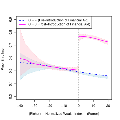
Figure 3: Enpirical Example: The Constant Bias Assumption Appears Valid

Of course, however, if the difference in the cutoff is correlated with underlying differences between groups (e.g., more generous cutoffs are set for minority, disadvantaged groups), the validity of the constant bias assumption is no longer guaranteed even when the running variable is effort-invariant. Hence, when applying the Cattaneo et al.,’s (2021) method, we recommend that a researcher justifies the similarity in unobservables between the two groups when the running variable is effort-invariant. Performing a balance test on observed covariates among the groups may provide reasonable indirect evidence.

2.2.2 Effort-Contingent Running Variable Case

Next, we consider the effort-contingent running variable case (2.3b). An important difference from the effort-invariant running variable case is characterized in the Proposition 2 below. We write the density function of $\eta_{i}^{s}$ by $f_{\eta^{s}}$, and assume the following conditions:

Assumption 2.3.

Suppose that the following conditions hold:

• $u\left(s(e_{i})\right)+\beta\left\{y(e_{i})+\tilde{\tau}\mathbb{P}\left[s(e_{i})+\eta_{i}^{s}\geq C_{i}\right]\right\}$ is strictly concave in $e_{i}$,

• $K(e_{i},\epsilon_{i})$ is convex in $e_{i}$,

• $u\left(s(e_{i})\right)$, $K(e_{i},\epsilon_{i})$, $y(e_{i})$, $s(e_{i})$, and $\mathbb{P}\left[s(e_{i})+\eta_{i}^{s}\geq C_{i}\right]$ are continuously differentiable in $e_{i}$.

Proposition 2.

Suppose that the running variable is effort-contingent and that Assumption 2.3 is satisfied. Then the optimal effort $e_{i}^{*}$ does not depend on $C_{i}$ for any $\epsilon_{i}$ if and only if the density function $f_{\eta^{s}}$ is periodic with period $h-l$, i.e., $f_{\eta^{s}}(z)=f_{\eta^{s}}(z+h-l)$, on the interval $[l-b,h-a]$, where $a$ ($b$) denotes the infimum (supremum) of $s(e_{i})$. ∎

In most applications, it is natural to assume that $l<b=\sup s(e_{i})$ and $\inf s(e_{i})=a<h$, that is, $l-b<0<h-a$. Now, recalling that $f_{\eta^{s}}$ represents the density of the stochastic shocks on the score variable, it would be more natural to assume that it is not periodic and instead resembles a unimodal density centered at zero, such as the Gaussian errors. Therefore, the proposition states that the optimal effort depends on the position of the cutoff in most cases.

An implication from Proposition 2 is that the effort input does differ in general, even when the distribution of $\epsilon_{i}$ is identical across groups. Hence, in contrast to the effort-invariant running variable case, the validity of the constant bias assumption is not ensured by the similarity of the groups. Of course, the dependence of $e_{i}^{*}$ on $C_{i}$ does not rule out the possibility that the constant bias assumption holds; however, motivating and justifying this assumption in practice could be rather challenging, since its validity depends on the functional forms of the structural functions, which are not observable by economists. Besides, the validity of the assumption becomes more unclear when the distribution of $\epsilon_{i}$ is supposed to differ. Furthermore, the examples below illustrate that simple and common specifications can lead to a substantial deviation from constancy.

Example 1.

Suppose that $u\left(s(e_{i})\right)=s(e_{i})=5\sqrt{e_{i}}$, $y(e_{i})=10\sqrt{e_{i}}$, and $K(e_{i},\epsilon_{i})=15(2-\epsilon_{i})e_{i}$. The distribution of $\eta_{i}^{s}$ is triangle, i.e., $f_{\eta^{s}}(z)=(1-|z|)_{+}$, which is made to obtain an explicit solution. The ability $\epsilon$ follows the uniform distribution, $\text{Uniform}(0,1)$. The cutoffs are $C_{i}\in\{2,3\}$. We set $\tilde{\tau}=1$ for $c\in\{2,3\}$, $\gamma=0$, and $\beta=1$. Under this setup, the optimal effort can be computed as

$$e_{i}^{*}=\begin{cases}\dfrac{1}{4(2-\epsilon_{i})^{2}}&\text{ if }\,\epsilon_{i}\leq\dfrac{4C_{i}-9}{2(C_{i}-1)}\text{ or }\,\dfrac{4C_{i}-1}{2(C_{i}+1)}<\epsilon_{i}\\ \dfrac{(4+C_{i})^{2}}{(17-6\epsilon_{i})^{2}}&\text{ if }\,\dfrac{6C_{i}-10}{3C_{i}}<\epsilon_{i}\leq\dfrac{4C_{i}-1}{2(C_{i}+1)}\\ \dfrac{(4-C_{i})^{2}}{(7-6\epsilon_{i})^{2}}&\text{ if }\,\dfrac{4C_{i}-9}{2(C_{i}-1)}<\epsilon_{i}\leq\dfrac{6C_{i}-10}{3C_{i}}\end{cases},$$ (2.4)

which confirms the dependence of $e_{i}^{*}$ on $C_{i}$. Plugging in this optimal effort to $s(e_{i})$ and $y(e_{i})$, we can compute the conditional expectations $\mathbb{E}\left[Y_{i}(0)|X_{i}\right]$ for each group, which are shown in Figure 4(a). It is obvious that the constant bias assumption is not satisfied, even though the two groups are similar in their ability and face the same decision problem except for the cutoff points.

Example 2.

Suppose the same structural functions as Example 1. We here assume that the group with $C_{i}=3$ is more advantaged in that the ability $\epsilon$ for the group with $C_{i}=3$ follows $\text{Uniform}(2/3,5/3)$. The optimal effort is determined by (2.4). The regression functions are shown in Figure 4(b). The constant bias assumption is, again, not satisfied.

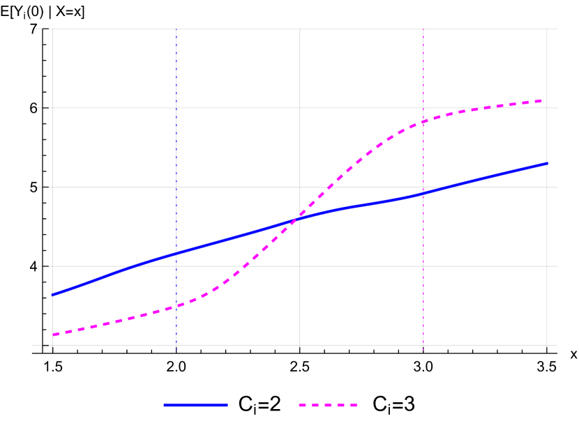
(a) Example 1

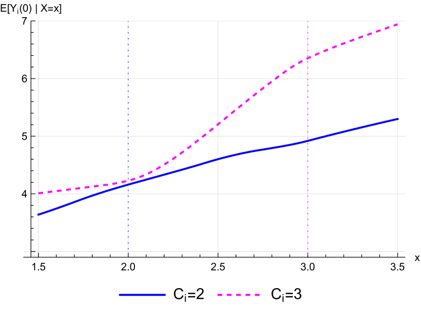
(b) Example 2

Figure 4: $\mathbb{E}\left[Y_{i}(0)|X_{i}=x\right]$ in Numerical Examples: Effort-Contingent Running Variable

As illustrated in the examples above, even when all determinants except the cutoff are the same between two groups, the resulting regression functions can differ substantially when the running variable is effort-contingent. This raises concerns about extrapolating treatment effects under the constant bias assumption in empirical applications with an effort-contingent running variable, where the functional forms of the structural functions are uncertain, making it challenging to justify constancy.

3 Alternative Identification

3.1 Assumptions and Identification

In the previous section, we observed several scenarios where the constant bias assumption may be violated. It suggests that, in some context, the extrapolation (2.1) under Assumption 2.2 could be biased. Hence, it would be useful to consider an alternative identification strategy that could be applied when Assumption 2.2 appears implausible. In this subsection, we introduce a different set of assumptions and develop identification under them to provide a practical complementary strategy, which is applicable even when the constant bias assumption fails.

The assumptions and identification results will be presented in statistical terms, as they may be applicable beyond the model discussed in the previous section and are more accessible to applied statisticians and empirical researchers across related fields; the relation to the model will be briefly mentioned as well.

We begin by introducing a functional form assumption:

Assumption 3.1 (Monotonicity).

$\mu_{0,l}(x)$ is weakly increasing in $x\in(l,h)$.

This monotonicity assumption states that the regression function without treatment is a monotone function in the running variable. This kind of monotonicity is commonly assumed in the partial identification literature (e.g., Manski,, 1997; González,, 2005).

This assumption will be plausible in many RD settings, as Babii and Kumar, (2023) wrote, “[r]egression discontinuity designs encountered in empirical practice are frequently monotone.” For example, when $X_{i}$ is the test score and $Y_{i}(0)$ represents future earnings without any treatment, it will be natural to assume that $\mu_{0,l}(x)$ is increasing. Similarly, when $X_{i}$ is the family income level and $Y_{i}(0)$ is again future earnings, it is reasonable to assume that $\mu_{0,l}(x)$ is increasing, as those with higher family income might inherit greater talent or benefit from human capital investment by their parents (Björklund et al.,, 2006). Furthermore, by interpreting these intuitions as $f_{\epsilon|X}^{l}(\epsilon|x^{\prime})\succeq_{1}f_{\epsilon|X}^{l}(\epsilon|x),x<x^{\prime}$, where $f_{\epsilon|X}^{c}$ is the conditional density of $\epsilon_{i}$ given $X_{i}$ for group $c$ and $\succeq_{1}$ denotes the first-order stochastic dominance, we can indeed obtain Assumption 3.1-(a) by assuming that $y(e_{i})$ in the decision model is an increasing function and additional regularity conditions hold (see Lemma 1 in Appendix A).

Our second assumption restricts the relationship between the regression functions of the two groups in a different way from the constant bias assumption, making it easier to discuss its empirical validity:

Assumption 3.2 (Dominance).

$\mu_{0,l}(x)\leq\mu_{0,h}(x)$ holds on $x\in(l,h)$.

This dominance assumption states that, without treatment, the regression function of one group lies above (or below) that of the other group.

The dominance assumption is also reasonable in many multi-cutoff RD settings. This is because the multiple cutoffs are often deliberately set to reduce disparities or emerge when there are differences between groups, such as in situations where lower test scores are required to receive scholarships for students from areas with a high poverty rate (Melguizo et al.,, 2016) or where well-prepared students aim for competitive schools with higher admission thresholds (Beuermann et al.,, 2022). Furthermore, these advantaged students may also benefit from additional factors, such as positive peer effects, as documented by Zimmerman, (2019). In such cases, Assumption 3.2-(a) is likely to be reasonable. By interpreting differences in ability or opportunity as $f_{\epsilon|X}^{h}(\epsilon|x)\succeq_{1}f_{\epsilon|X}^{l}(\epsilon|x)$ and the positive peer effect as a positive, large $\gamma$, we obtain Assumption 3.2-(a) provided that $y(e_{i})$ is increasing and regularity conditions hold (Lemma 1 in Appendix A).

We argue that these empirically motivated assumptions can be an alternative to the constant bias assumption. Formally, we have the following identification result:

Theorem 1 (Bounds on Extrapolated RD Effects).

Under Assumptions 2.1, 3.1, and 3.2, the treatment effect for group $C_{i}=l$ on $\bar{x}\in(l,h)$, $\tau_{l}(\bar{x})$, can be bounded from below and above by

$$\rotatebox[origin={c}]{180.0}{$\nabla$}_{l}(\bar{x})=\mu_{1,l}(\bar{x})-\mu_{0,h}(\bar{x}),\,\,\nabla_{l}(\bar{x})=\mu_{1,l}(\bar{x})-\mu_{0,l}(l).$$

These bounds $[\rotatebox[origin={c}]{180.0}{$\nabla$}_{l}(\bar{x}),\nabla_{l}(\bar{x})]$ are sharp. ∎

Corollary 1.

Suppose the “reverse” of Assumptions 3.1 and 3.2 hold instead; that is, $\mu_{0,l}(x)$ is weakly decreasing and $\mu_{0,l}(x)\geq\mu_{0,h}(x)$ on $x\in(l,h)$. Then, the sharp bounds are give by $[\nabla_{l}(\bar{x}),\rotatebox[origin={c}]{180.0}{$\nabla$}_{l}(\bar{x})]$. ∎

The idea of this identification result is illustrated in Figure 5. By Assumption 3.1, we can bound the unobservable $\mu_{0,l}(\bar{x})$ from below by $\mu_{0,l}(l)$. The upper bound on $\mu_{0,l}(\bar{x})$ is $\mu_{0,h}(\bar{x})$ due to Assumption 3.2. Hence, we obtain that $\tau_{l}(\bar{x})\in[\rotatebox[origin={c}]{180.0}{$\nabla$}_{l}(\bar{x}),\nabla_{l}(\bar{x})]$. The obtained bounds can be a useful tool when a researcher is uncertain about the empirical validity of the constant bias assumption.

Figure 5: Bounds of Theorem 1

We conclude this subsection with a few important remarks:

Remark 1 ((Non-)Sensitivity to Transformation).

In RD studies, it is common practice to apply a monotonic transformation to the outcome variable (e.g., log transformation of annual earnings as in Oreopoulos,, 2006). The constant bias assumption can be sensitive to such transformations. This type of sensitivity to transformations has been pointed out by Roth and Sant’Anna, (2023) in the difference-in-differences setting. Our identification conditions, Assumptions 3.1 and 3.2, are not subject to this sensitivity. Therefore, the bounds are also useful when researchers are interested in the transformed variable but the plausibility of the constant bias assumption for the transformed variable is unclear. ∎

Remark 2 (Effect of Changing Threshold).

$\tau_{l}(\bar{x})$ should be understood as the treatment effect in an economy where agents make decisions with the cutoff point set at $l$. Consequently, when an economist is interested in the effect of shifting the threshold from $l$ to $\bar{x}$, $\tau_{l}(\bar{x})$ may not serve as a particularly useful parameter. To interpret $\tau_{l}(\bar{x})$ in this context, a policy invariance assumption, akin to the local policy invariance assumption in Dong and Lewbel, (2015), becomes necessary. Formally, we must assume that the treatment effect function remains unaffected by the cutoff point, such that $\tau_{l}(\bar{x})=\tau(\bar{x})$ for $\bar{x}\in(l,h)$. Under this assumption, the derived bounds represent valid bounds on the effect of adjusting the threshold to $\bar{x}$. ∎

Remark 3 (Limitation of the Multi-Cutoff RD Designs).

Our bounds do not provide any information about $\tau_{l}(x)$ on $x<l$, which may also be a parameter of interest. This limitation is similar to the issue discussed in Cattaneo et al., (2021, p. 1947). Exploring strategies for this case will be an important direction, though we leave it for a future study. We should note that the local extrapolation strategy proposed by Dong and Lewbel, (2015) is applicable even in this case. ∎

3.2 Estimation and Inference

In this section, we provide estimation and inference procedures, both of which are not complicated and are rather simple. The unknown quantities $\mu_{1,l}(\bar{x})$, $\mu_{0,h}(\bar{x})$, and $\mu_{0,l}(l)$ are all consistently estimable by standard nonparametric regression techniques. Following the recent RD literature, we propose to estimate $\mu_{d,c}(x)$ using the local linear smoothing and a mean-squared error optimal bandwidth selector (see Fan and Gijbels,, 1996 for a review). Let $\widehat{\mu}_{d,c}(x)$ denote the estimator. Then we can estimate the bounds by $\widehat{\rotatebox[origin={c}]{180.0}{$\nabla$}}_{l}(\bar{x})=\widehat{\mu}_{1,l}(\bar{x})-\widehat{\mu}_{0,h}(\bar{x})$ and $\widehat{\nabla}_{l}(\bar{x})=\widehat{\mu}_{1,l}(\bar{x})-\widehat{\mu}_{0,l}(l)$.

For inference, the robust bias-corrected procedure, which corrects for smoothing bias and accounts for the variance introduced by this bias estimation, as developed by Calonico et al., (2014, 2018), must be useful. Let $B_{d,c}(x)$ be the asymptotic smoothing bias, which can be estimated using local quadratic regression, producing the estimator $\widehat{B}_{d,c}(x)$. Then, by defining $\mathcal{V}_{d,c}(x)=\mathbb{V}\left[\widehat{\mu}_{d,c}(x)-\widehat{B}_{d,c}(x)|X_{1},\ldots,X_{n}\right]$ and letting $\widehat{\mathcal{V}}_{d,c}(x)$ be its estimator, we have that

$$\frac{\widehat{\mu}_{d,c}^{\text{BC}}(x)-{\mu}_{d,c}(x)}{\sqrt{\widehat{\mathcal{V}}_{d,c}(x)}}\to_{d}\mathcal{N}(0,1),$$

where $\widehat{\mu}_{d,c}^{\text{BC}}(x)=\widehat{\mu}_{d,c}(x)-\widehat{B}_{d,c}(x)$ and $\to_{d}$ denotes the convergence in distribution, which is shown in Calonico et al., (2014, 2018) under suitable smoothness and regurality conditions. By putting $\widehat{\rotatebox[origin={c}]{180.0}{$\nabla$}}_{l}^{\text{BC}}=\widehat{\mu}_{1,l}^{\text{BC}}(\bar{x})-\widehat{\mu}_{0,h}^{\text{BC}}(\bar{x})$, $\widehat{\nabla}_{l}^{\text{BC}}=\widehat{\mu}_{1,l}^{\text{BC}}(\bar{x})-\widehat{\mu}_{0,l}^{\text{BC}}(l)$, since $\widehat{\mu}_{1,l}^{\text{BC}}(\bar{x})$, $\widehat{\mu}_{0,h}^{\text{BC}}(\bar{x})$, and $\widehat{\mu}_{0,l}^{\text{BC}}(l)$ are independent by the assumption of random sampling, $\widehat{\rotatebox[origin={c}]{180.0}{$\nabla$}}_{l}^{\text{BC}}(\bar{x})$ and $\widehat{\nabla}_{l}^{\text{BC}}(\bar{x})$ are jointly asymptotically normal with the asymptotic variances $\widehat{\mathcal{V}}_{L}=\widehat{\mathcal{V}}_{1,l}(\bar{x})+\widehat{\mathcal{V}}_{0,h}(\bar{x})$, and $\widehat{\mathcal{V}}_{U}=\widehat{\mathcal{V}}_{1,l}(\bar{x})+\widehat{\mathcal{V}}_{0,l}(l)$. Then we can construct Imbens and Manski,’s (2004) confidence interval (CI) with an asymptotic coverage rate of at least $1-\alpha$:

$$\left[\widehat{\rotatebox[origin={c}]{180.0}{$\nabla$}}_{l}^{\text{BC}}-C_{n}\sqrt{\widehat{\mathcal{V}}_{L}},\widehat{\nabla}_{l}^{\text{BC}}+C_{n}\sqrt{\widehat{\mathcal{V}}_{U}}\right],$$

where $C_{n}$ satisfies

$$\Phi\left(C_{n}+\frac{\widehat{\nabla}_{l}^{\text{BC}}-\widehat{\rotatebox[origin={c}]{180.0}{$\nabla$}}_{l}^{\text{BC}}}{\max\left\{\widehat{\mathcal{V}}_{L},\widehat{\mathcal{V}}_{U}\right\}}\right)-\Phi(-C_{n})=1-\alpha$$

and $\Phi(\cdot)$ is the distribution function of the standard Gaussian distribution. In the empirical illustrations in Section 4, we set $\alpha=0.05$. The proposed estimation and inference procedures can be implemented by a ready-to-use R program included in the replication file. In the Online Appendix, we conduct simulation studies and confirm the excellent performance of the proposed procedure in terms of the accuracy of the bounds estimates, as well as the coverage rate and power of the CIs.

4 Empirical Illustrations

In this section, we present two empirical applications to illustrate the implication of the constant bias assumption from Section 2 and demonstrate the potential usefulness of the bounds derived in the previous sections. First, in Section 4.1, we consider a financial aid program setting, originally studied by Londoño-Vélez et al., (2020), wherein the running variable is effort-invariant. Then, in Section 4.2, we revisit the empirical analysis in Cattaneo et al., (2021), wherein the running variable is effort-contingent. We focus on the sharp RD case in both applications for ease of intuition. In the Online Appendix, we provide an empirical illustration of the fuzzy RD case using bounds obtained later in Section 5.

4.1 SPP Program (Effort-Invariant Case)

We investigate the effect of a financial aid program, Ser Pilo Page (SPP), introduced in Columbia in 2014. Students have to meet both merit- and need-based criteria to qualify for full scholarship loans from SPP, with program eligibility determined by test scores and family wealth level index. Londoño-Vélez et al., (2020) leveraged these eligibility criteria to estimate the standard RD effects on the enrollment rate to higher education. In the following analysis, following Londoño-Vélez et al., (2020), we will focus on merit-eligible students—those whose test scores are above the minimum requirement—and estimate the “frontier-specific” RD effect on the enrollment rate. Note that the merit-based cutoff is the same for all applicants.

Now, the running variable is the wealth index, which ranges from $0$ (poorer) to $100$ (richer). Students whose index is below the region-specific cutoff are offered financial aid. Below, we multiply the wealth index by $-1$ to align with the stylized RD settings; a larger number indicates a poorer household.

In the SPP, the cutoff for students from metropolitan areas is $-57.21$ (richer) while that for rural areas is $-40.75$ (poorer), making a multi-cutoff RD setting. We focus on the intent-to-treat effects and postpone the issue of incomplete compliance to the Online Appendix, wherein a formal analysis utilizing Theorem 2 in Section 5 is provided.

In this scenario, the constant bias assumption of Cattaneo et al., (2021) may be somewhat reasonable for some reasons. First, the running variable is effort-invariant. Second, while concerns remain about the constant bias assumption—given that the eligibility rule is progressive and the cutoff value is more generous for students from rural regions—focusing on merit-eligible students could help ensure a certain degree of similarity. This focus may make the constant bias assumption a reasonable approximation, thereby alleviating the concern.

Hence, we estimate the treatment effects at $\bar{x}\in\{-50,-45\}$ under the constant bias assumption. We also compute the bounds obtained in Corollary 1. As for the validity of the bounds, note that (the reverse of) Assumptions 3.1 and 3.2 seem reasonable in this context: It would be natural to assume that the probability of enrollment decreases as family wealth decreases, and we could also assume that the regression function for students from rural, disadvantaged areas lies below that for students living in metropolitan areas.

Table 1 reports the results under the constant bias assumption, along with the bounds obtained in Corollary 1; see also Figure 6(a) for estimated regression functions. We observe that the bounds are tight enough, and the point estimates under the constant bias assumption fall within these bounds. Together, these findings indicate a certain degree of plausibility for extrapolation under the constant bias assumption, as well as the practical usefulness of the bounds.

Table 1: Empirical Bounds: SPP

	(1)	(2)	(3)	(4)
	Cattaneo et al., (2021)	LB	UB	$95\%$ CI
$\bar{x}=-50$	$0.222$	$0.203$	$0.253$	$(0.138,0.309)$
	$(0.108,0.316)$	$(0.038)$	$(0.030)$
$\bar{x}=-45$	$0.221$	$0.195$	$0.252$	$(0.137,0.363)$
	$(0.141,0.382)$	$(0.038)$	$(0.033)$

Note: $n=20551$. The first column indicates the extrapolated effects under the constant bias assumption with the robust bias-corrected $95\%$ CIs in the parenthesis. In the second and third columns (LB, UB), the estimated lower and upper bounds are shown with standard errors in the parenthesis. The fourth column shows Imbens and Manski,’s (2004) CIs.

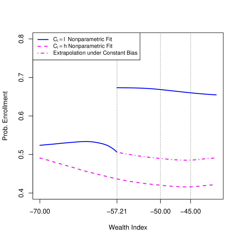
(a) SPP

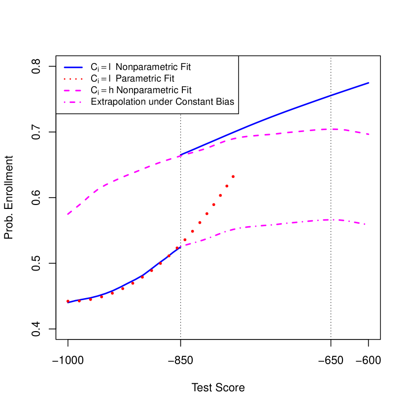
(b) ACCES

Figure 6: Estimated Regression Functions in Empirical Illustrations

4.2 ACCES Program (Effort-Contingent Case)

We examine the effect of the Acceso con Calidad a la Educación Superior (ACCES) program, a national-level merit-based financial aid initiative, on Colombian students’ higher education enrollment. To be eligible for ACCES, students must score below a certain threshold on the national high school exit examination. The test score ranges from $1$ (best) to $1000$ (worst), and the cutoff was $850$ before 2008. In 2009, the cutoff began to differ across geographic regions, creating a multi-cutoff RD setting.

Cattaneo et al., (2021) utilized these multiple cutoffs to estimate the extrapolated RD effect on the probability of enrollment in higher education. The study focused on two populations of students: Those who applied for ACCES between 2000 and 2008, for whom the cutoff was $-850(=l)$, and those who applied between 2009 and 2010 in regions where the cutoff was $-571(=h)$. Cattaneo et al., (2021) was interested in estimating the treatment effect at $-650(=\bar{x})$. Their estimation was performed under the constant bias assumption, and they found that $\widehat{\tau}_{-850,\text{CB}}(-650)=0.191$, reproduced in Table 2.

Unfortunately, several concerns about the plausibility of the constant bias assumption exist. First, the running variable is effort-contingent. In addition, the cutoffs after 2009 were determined in a progressive fashion, meaning more lenient requirements were set for students from disadvantaged regions, while stricter thresholds were set for students from advantaged regions. In fact, the region with a cutoff of $-571$ is substantially advantaged, with a very low proportion of low socio-economic status students (Melguizo et al.,, 2016, Figure 1). Therefore, the similarity between the two groups may not be very plausible. For these reasons, the constant bias assumption can fail in light of our discussion in Section 2.

Second, we visually assess the plausibility of the constant bias assumption in Figure 6(b). The pink, dot-dashed line is constructed from extrapolation under the constant bias assumption, and we also draw the parametric extrapolated line (red, dotted line) just above the lower cutoff, which is modeled as a quadratic function following Cattaneo et al., (2021). Then, we observe a substantial difference in the slope of these two lines, even just above the cutoff, which may suggest that the ”parallel trend” assumption does not hold.

Even if the constant bias assumption is violated, our bounding approach will still be valid. In this setting, it is reasonable to assume that the enrollment probability increases with higher test scores and is higher for students from advantaged regions. Hence, we estimate the bounds $[\rotatebox[origin={c}]{180.0}{$\nabla$}_{l}(\bar{x}),\nabla_{l}(\bar{x})]$.

The estimated bounds are reported in Table 2.

Table 2: Empirical Bounds: ACCES

	(1)	(2)	(3)	(4)
	Cattaneo et al., (2021)	LB	UB	$95\%$ CI
$\bar{x}=-650$	$0.191$	$0.050$	$0.231$	$(-0.01,0.313)$
	$(0.081,0.332)$	$(0.032)$	$(0.042)$

Note: $n=1365$. The first column indicates the extrapolated effect under the constant bias assumption with the robust bias-corrected $95\%$ CIs in the parenthesis. In the second and third columns (LB, UB), the estimated lower and upper bounds are shown with standard errors in the parenthesis. The fourth column shows Imbens and Manski,’s (2004) CIs.

The bounds and the associated CI suggest that while the treatment effect of the ACCES program remains positive, it can be substantially smaller for students with higher test scores. This scenario could be plausible, as students with lower test scores in 2000-2008 might differ significantly from those with higher scores in terms of socio-economic background, such as family income or housing region. Specifically, before the policy change, students with $X_{i}=-650$ could be more likely to come from advantaged families compared to those with $X_{i}=-850$. Consequently, their enrollment rate in the absence of financial aid could be much higher than that of students near the lower cutoff, potentially resulting in a smaller treatment effect from the financial aid. In such cases, the magnitude of the effect near the lower bound could be attained. As a result, we could not reject the possibility that the treatment effect at $\bar{x}=-650$ can differ from, and much smaller than, the large positive effect at $x=-850$.

5 Extention to One-Sided Fuzzy Multi-Cutoff RD

Following Cattaneo et al., (2021), we consider the fuzzy RD designs where one-sided noncompliance may occur: Someone with $X_{i}\geq C_{i}$ is not necessarily treated, while nobody with $X_{i}<C_{i}$ is treated. This case will be of empirical importance as many programs in RD settings fit this scenario; for example, those below the eligibility cutoff cannot gain a financial aid offer, while offered students may opt not to receive the scholarship (Londoño-Vélez et al.,, 2020). If this one-sided noncompliance assumption fails, additional information about the compliance types is necessary, but we postpone such investigation to future work.

We now redefine the treatment indicator as $D_{i}(x,c)\in\{0,1\}$ and assume the following conditions, which are assumed in Cattaneo et al., (2021, Assumption 3):

Assumption 5.1 (One-Sided Compliance Fuzzy RD).

The following conditions hold:

• $\mathbb{E}\left[Y_{i}(0)|X_{i}=x,C_{i}=c\right]$ and $\mathbb{E}\left[\{Y_{i}(1)-Y_{i}(0)\}D_{i}(x,c)|X_{i}=x,C_{i}=c\right]$ are continuous in $x$ for all $c\in\{l,h\}$,

• $D_{i}(x,c)=0$ for all $x<c$.

Under Assumptions 2.2 and 5.1, Cattaneo et al., (2021) shows that the following “LATE-type” parameter,

$$\tau_{l}^{f}(\bar{x})=\mathbb{E}\left[Y_{i}(1)-Y_{i}(0)|X_{i}=\bar{x},C_{i}=l,D_{i}(\bar{x},l)=1\right],$$

is identified as follows:

$$\tau_{l,\text{CB}}^{f}(\bar{x})=\frac{\mu_{l}(\bar{x})-\mu_{h}(\bar{x})+B(l)}{\mathbb{E}\left[D_{i}(\bar{x},l)|X_{i}=\bar{x},C_{i}=l\right]},$$

for all $\bar{x}\in(l,h)$, where $\mu_{c}(x)=\mathbb{E}\left[Y_{i}|X_{i}=x,C_{i}=c\right]$.

As discussed in previous sections, Assumption 2.2 may not be plausible in some situations. However, we can again obtain useful bounds under Assumptions 3.1 and 3.2.

Theorem 2 (Bounds on Extrapolated Fuzzy RD Effects).

Under Assumptions 3.1, 3.2, and 5.1, $\tau_{l}^{f}(\bar{x}),\bar{x}\in(l,h)$, can be bounded from below and above by

$$\rotatebox[origin={c}]{180.0}{$\nabla$}_{l}^{f}(\bar{x})=\frac{\mu_{l}(\bar{x})-\mu_{h}(\bar{x})}{\mathbb{E}\left[D_{i}(\bar{x},l)|X_{i}=\bar{x},C_{i}=l\right]},\,\,\nabla_{l}^{f}(\bar{x})=\frac{\mu_{l}(\bar{x})-\lim_{x\uparrow l}\mu_{l}(x)}{\mathbb{E}\left[D_{i}(\bar{x},l)|X_{i}=\bar{x},C_{i}=l\right]}.$$

These bounds $[\rotatebox[origin={c}]{180.0}{$\nabla$}_{l}^{f}(\bar{x}),\nabla_{l}^{f}(\bar{x})]$ are sharp. ∎

Estimation can be performed in a similar way to Section 3.2. The inference procedure is also similar to before, thanks to Slutsky’s theorem. The replication package also includes an R program for the fuzzy case.

6 Conclusion

This paper explored when and how the treatment effect in RD designs can be extrapolated away from cutoff points in multi-cutoff settings. We began by examining the plausibility of the constant bias assumption proposed by Cattaneo et al., (2021) through the lens of rational decision-making behavior. We found that this assumption is reasonable if the two groups consist of similar agents and when the running variable is effort-invariant. However, this positive conclusion is not maintained when the running variable is contingent on the agents’ effort, perhaps leading to a substantially biased estimate. To address this issue, we introduced alternative assumptions grounded in empirical motivations and derived a new partial identification result that does not rely on the constant bias assumption. We further extended the proposed bounds to the fuzzy RD setting. The empirical examples underscore the potential applicability and usefulness of these bounds.

Appendix A Proofs

• This is an immediate consequence of (2.3a). ∎

• Let $e_{c}^{*}(\epsilon_{i})$ denote the optimal effort of those with $\epsilon_{i}$ in the group $c\in\{l,h\}$. Take an arbitrary $\epsilon_{i}$ and suppose $e_{l}^{*}(\epsilon_{i})=e_{h}^{*}(\epsilon_{i})=:e_{i}^{*}$. Then, by the first-order condition, we have

  $$u^{\prime}\left(s(e_{i}^{*})\right)s^{\prime}(e_{i}^{*})-\frac{\partial K}{\partial e}(e_{i}^{*},\epsilon_{i})+\beta(y^{\prime}(e_{i}^{*})+\tilde{\tau}s^{\prime}(e_{i}^{*})f_{\eta^{s}}(l-s(e_{i}^{*})))$$

  $$\quad=u^{\prime}(s(e_{i}^{*})s^{\prime}(e_{i}^{*})-\frac{\partial K}{\partial e}(e_{i}^{*},\epsilon_{i})+\beta(y^{\prime}(e_{i}^{*})+\tilde{\tau}s^{\prime}(e_{i}^{*})f_{\eta^{s}}(h-s(e_{i}^{*})))=0$$

  $$\Longleftrightarrow f_{\eta^{s}}(l-s(e_{i}^{*}))=f_{\eta^{s}}(h-s(e_{i}^{*})).$$

  As $e_{i}^{*}$ is continuous in $\epsilon_{i}$ by the implicit function theorem, $f_{\eta^{s}}$ is periodic with period $h-l$ on the interval $[l-b,h-a]$.

  Conversely, suppose that $f_{\eta^{s}}$ is periodic with period $h-l$, then we have for any $e_{i}$,

  $$\mathbb{P}\left[s(e_{i})+\eta_{i}^{s}\geq l\right]=\mathbb{P}\left[s(e_{i})+\eta_{i}^{s}\geq h\right]+D,$$

  where $D=\int_{l-b}^{h-b}f_{\eta_{s}}(z)\,dz$. Therefore, the decision problem for group $l$ can be rewritten as

  $$\max_{e_{i}}\bigg{[}u\left(s(e_{i})\right)-K(e_{i},\epsilon_{i})+\beta\big{\{}y(e_{i})+\tilde{\tau}\mathbb{P}\left[s(e_{i})+\eta_{i}^{s}\geq l\right]\big{\}}\bigg{]}$$

  $$=\max_{e_{i}}\bigg{[}u\left(s(e_{i})\right)-K(e_{i},\epsilon_{i})+\beta\left\{y(e_{i})+\tilde{\tau}\left(\mathbb{P}\left[s(e_{i})+\eta_{i}^{s}\geq h\right]+D\right)\right\}\bigg{]},$$

  which is equivalent to

  $$\max_{e_{i}}\bigg{[}u\left(s(e_{i})\right)-K(e_{i},\epsilon_{i})+\beta\big{\{}y(e_{i})+\tilde{\tau}\mathbb{P}\left[s(e_{i})+\eta_{i}^{s}\geq h\right]\big{\}}\bigg{]}.$$

  This is the decision problem for group $h$. Hence, the decision problems are essentially the same between the two groups, which implies that the optimal effort $e_{i}^{*}$ does not depend on $C_{i}$ for any $\epsilon_{i}$. ∎

Lemma 1.

Suppose Assumption 2.3 and $\partial^{2}K(e_{i},\epsilon_{i})/\partial e_{i}\partial\epsilon_{i}\leq 0$. Then $e_{i}^{*}(\epsilon_{i})$ is weakly increasing in $\epsilon_{i}$. Consequently, $y\left(e_{i}^{*}(\epsilon_{i})\right)$ is weakly increasing in $\epsilon_{i}$ if $y(e_{i})$ is weakly increasing in $e_{i}$. ∎

• For some $\epsilon_{0},\epsilon_{1}(\epsilon_{0}<\epsilon_{1})$, suppose $e_{i}^{*}(\epsilon_{0})>e_{i}^{*}(\epsilon_{1})$. By the first-order condition,

  $$U^{\prime}(e_{i}^{*}(\epsilon))=\frac{\partial K}{\partial e_{i}}(e_{i}^{*}(\epsilon),\epsilon),$$

  where $U(e_{i}):=u\left(s(e_{i})\right)+\beta\left\{y(e_{i})+\tilde{\tau}\mathbb{P}\left[s(e_{i})+\eta_{i}^{s}\geq C_{i}\right]\right\}$. Then, we have

  $$U^{\prime}(e_{i}^{*}(\epsilon_{0})) <U^{\prime}(e_{i}^{*}(\epsilon_{1}))$$

  $$=\frac{\partial K}{\partial e_{i}}(e_{i}^{*}(\epsilon_{1}),\epsilon_{1})$$

  $$\leq\frac{\partial K}{\partial e_{i}}(e_{i}^{*}(\epsilon_{0}),\epsilon_{1})$$

  $$\leq\frac{\partial K}{\partial e_{i}}(e_{i}^{*}(\epsilon_{0}),\epsilon_{0}),$$

  where the first inequality uses the strict concavity of $U$, the equality is due to the first-order condition, the second inequality uses the convexity of $K$, and the last inequality comes from ${\partial^{2}K}/{\partial\epsilon_{i}\partial e_{i}}\leq 0$. However, this relationship contradicts the first-order condition in $\epsilon_{0}$, which proves that $e_{i}^{*}(\epsilon_{i})$ is weakly increasing in $\epsilon_{i}$. By this result, we find that $y\left(e_{i}^{*}(\epsilon_{i})\right)$ is weakly increasing in $\epsilon_{i}$ if $y(e_{i})$ is weakly increasing in $e_{i}$. ∎

• The validity of the bounds is illustrated in the main text. Hence, it suffices to show the sharpness. Fix $\bar{x}\in(l,h)$ arbitrarily. Suppose $\mu_{0,l}(x)=\mu_{0,l}(l)$ on $x\in(l,h)$. Then, Assumptions 2.1, 3.1, and 3.2 hold, and the upper bound $\nabla_{l}(\bar{x})$ is attained. Suppose instead that

  $$\mu_{0,l}(x)=\begin{cases}\frac{\mu_{0,h}(\bar{x})-\mu_{0,l}(l)}{\bar{x}-l}(x-l)+\mu_{0,l}(l)&\text{ if }l<x<\bar{x}\\ \mu_{0,h}(x)&\text{ if }x\geq\bar{x}\end{cases}.$$

  Then, Assumptions 2.1, 3.1, and 3.2 again hold, and the lower bound $\rotatebox[origin={c}]{180.0}{$\nabla$}_{l}(\bar{x})$ is attained. These show that the endpoints of the bounds are attainable, i.e., the bounds are sharp. ∎

• As $D_{i}(x,c)\in\{0,1\}$,

  $$\mathbb{E}\left[Y_{i}(d)D_{i}(x,c)|X_{i}=x,C_{i}=c\right]$$

  $$\quad=\mathbb{E}\left[Y_{i}(d)|X_{i}=x,C_{i}=c,D_{i}(x,c)=1\right]\mathbb{E}\left[D_{i}(x,c)|X_{i}=x,C_{i}=c\right],$$

  and then we have that

  $$\tau_{l}^{f}(\bar{x})=\frac{\mathbb{E}\left[\left\{Y_{i}(1)-Y_{i}(0)\right\}D_{i}(\bar{x},l)|X_{i}=\bar{x},C_{i}=l\right]}{\mathbb{E}\left[D_{i}(\bar{x},l)|X_{i}=\bar{x},C_{i}=l\right]}.$$

  Here, we can compute that

  $$\mu_{l}(\bar{x}) =\mathbb{E}\left[Y_{i}(1)D_{i}(\bar{x},l)+Y_{i}(0)\left(1-D_{i}(\bar{x},l)\right)|X_{i}=\bar{x},C_{i}=l\right]$$

  $$=\mathbb{E}\left[\left\{Y_{i}(1)-Y_{i}(0)\right\}D_{i}(\bar{x},l)|X_{i}=\bar{x},C_{i}=l\right]+\mu_{0,l}(\bar{x}),$$

  that is, $\mathbb{E}\left[\left\{Y_{i}(1)-Y_{i}(0)\right\}D_{i}(\bar{x},l)|X_{i}=\bar{x},C_{i}=l\right]=\mu_{l}(\bar{x})-\mu_{0,l}(\bar{x})$. By Assumptions 3.1 and 3.2, we can bound the second term as $-\mu_{0,h}(\bar{x})\leq-\mu_{0,l}(\bar{x})\leq-\mu_{0,l}(l)$. Plus, one-sided compliance ($\lim_{x\uparrow l}D_{i}(x,l)=0$ and $D_{i}(\bar{x},h)=0$) implies that

  $$-\mu_{h}(\bar{x})\leq-\mu_{0,l}(\bar{x})\leq-\lim_{x\uparrow l}\mu_{l}(x).$$

  Combining the equalities and inequalities above, we obtain the bounds. The sharpness can be shown in a similar way to the Proof of Theorem 1. ∎

Appendix S1 Additional Empirical Illustration

S1.1 SPP Program (Fuzzy RD)

In the main article, we investigated the effect of the SPP program. In reality, there was a compliance issue: Those with aid offers do not necessarily accept the offer, leading to the one-sided fuzzy RD setting. We thus compute the bounds obtained in Theorem 2.

The estimated bounds, shown in Table S1, suggest that the treatment effects at $-50$ and $-45$ are positive. Furthermore, the bounds are sufficiently narrow and we can see that the treatment effects would be similar in level.

Table S1: Empirical Bounds: SPP (Fuzzy RD)

	(1)	(2)	(3)	(4)
	Cattaneo et al., (2021)	LB	UB	$95\%$ CI
$\bar{x}=-50$	$0.591$	$0.542$	$0.675$	$(0.369,0.823)$
	$(0.289,0.842)$	$(0.100)$	$(0.080)$
$\bar{x}=-45$	$0.591$	$0.521$	$0.675$	$(0.366,0.970)$
	$(0.377,1.022)$	$(0.100)$	$(0.088)$

Note: $n=20551$. The first column indicates the extrapolated effect under the constant bias assumption with the robust bias-corrected $95\%$ CIs in the parenthesis. In the second and third columns (LB, UB), the estimated lower and upper bounds are shown with standard errors in the parenthesis. The fourth column shows Imbens and Manski,’s (2004) CIs.

Appendix S2 Numerical Studies

We perform simulation studies to investigate the finite-sample performance of the bounds. We suppose the sharp RD design. Let $X_{i}^{c}$ be the running variable of those in group $c\in\{l,h\}$, where $l=1$ and $h=2.25$. We assume $X_{i}^{l}$ and $X_{i}^{h}$ respectively follow the Gaussian distributions $\mathcal{N}\left(l,1\right)$ and $\mathcal{N}\left(h,1\right)$ truncated to the interval $(0.5,3.0)$. The outcomes are determined by the following equations:

$$Y_{i}^{l}(0) =-0.056X_{i}^{3}-0.099X_{i}^{2}+1.983X_{i}+0.296+\varepsilon_{i},$$

$$Y_{i}^{l}(1) =Y_{i}^{l}(0)+1.5,$$

$$Y_{i}^{h}(0) =-0.553X_{i}^{3}+2.335X_{i}^{2}-0.872X_{i}+1.439+\varepsilon_{i},$$

where $\varepsilon_{i}\sim\mathcal{N}(0,1)$; see also Figure S1.

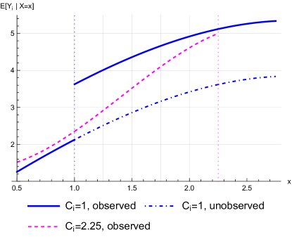
Figure S1: Conditional Expectations

We evaluate the four equispaced points between the cutoffs, $\bar{x}\in\{1.25,1.50,1.75,2.00\}$. Note that, by construction, the treatment effect at every point is $1.5$. We randomly generate the samples of size $n_{c}=500$ and $1000$ for each groups. With $1000$ repetation, we assess the performance of the bounds.

Table S2 reports the results. The point estimates of the bounds are all close to the theoretical values, the coverage probability is consistent with the asymptotic theory, and the power is also excellent at every evaluation points.

Table S2: Simulation Results

	LB	UB	Length of CIs	Coverage of CIs ($\%$)	$\%$ of $0\notin\text{CIs}$
$n_{c}=500$
$\bar{x}=1.25$	1.07	1.89	1.92	98.8	100
	(0.12)	(0.41)
$\bar{x}=1.50$	0.83	2.23	2.48	99.6	100
	(0.10)	(0.41)
$\bar{x}=1.75$	0.57	2.53	3.05	99.8	99.2
	(0.10)	(0.41)
$\bar{x}=2.00$	0.31	2.79	3.59	99.8	63.7
	(0.12)	(0.42)
$n_{c}=1000$
$\bar{x}=1.25$	1.07	1.88	1.59	99.6	100
	(0.09)	(0.27)
$\bar{x}=1.50$	0.83	2.22	2.13	100	100
	(0.08)	(0.27)
$\bar{x}=1.75$	0.57	2.52	2.71	100	100
	(0.08)	(0.27)
$\bar{x}=2.00$	0.31	2.77	3.24	100	86.1
	(0.09)	(0.28)

Note: The treatment effect is $1.5$ at every evaluation point. The theoretical values of lower bounds are in order $1.09,0.84,0.56,$ and $0.31$, and that of upper bounds are $1.89,2.23,2.54,$ and $2.79$. In the first column (LB), the averages of the estimated lower bounds are shown with standard errors in the parenthesis. The second column (UB) is for upper bounds. The third and fourth columns show the average length and empirical coverage of Imbens and Manski,’s CIs. In the last column, the percentage that the bounds do not include zero is reported.

References

- Abadie and Cattaneo, (2018) Abadie, A. and Cattaneo, M. D. (2018). Econometric Methods for Program Evaluation. Annual Review of Economics, 10:465–503.
- Angrist and Rokkanen, (2015) Angrist, J. D. and Rokkanen, M. (2015). Wanna Get Away? Regression Discontinuity Estimation of Exam School Effects Away From the Cutoff. Journal of the American Statistical Association, 110(512):1331–1344.
- Arai and Ichimura, (2016) Arai, Y. and Ichimura, H. (2016). Optimal Bandwidth Selection for the Fuzzy Regression Discontinuity Estimator. Economics Letters, 141:103–106.
- Arai and Ichimura, (2018) Arai, Y. and Ichimura, H. (2018). Simultaneous Selection of Optimal Bandwidths for the Sharp Regression Discontinuity Estimator. Quantitative Economics, 9(1):441–482.
- Babii and Kumar, (2023) Babii, A. and Kumar, R. (2023). Isotonic Regression Discontinuity Designs. Journal of Econometrics, 234(2):371–393.
- Bertanha and Imbens, (2020) Bertanha, M. and Imbens, G. W. (2020). External Validity in Fuzzy Regression Discontinuity Designs. Journal of Business & Economic Statistics, 38(3):593–612.
- Beuermann et al., (2022) Beuermann, D. W., Jackson, C. K., Navarro-Sola, L., and Pardo, F. (2022). What is a Good School, and Can Parents Tell? Evidence on the Multidimensionality of School Output. The Review of Economic Studies, 90(1):65–101.
- Björklund et al., (2006) Björklund, A., Lindahl, M., and Plug, E. (2006). The Origins of Intergenerational Associations: Lessons from Swedish Adoption Data. The Quarterly Journal of Economics, 121(3):999–1028.
- Brodeur et al., (2020) Brodeur, A., Cook, N., and Heyes, A. (2020). Methods Matter: p-Hacking and Publication Bias in Causal Analysis in Economics. American Economic Review, 110(11):3634–60.
- Bugni and Canay, (2021) Bugni, F. A. and Canay, I. A. (2021). Testing Continuity of a Density via G-order Statistics in the Regression Discontinuity Design. Journal of Econometrics, 221(1):138–159.
- Calonico et al., (2018) Calonico, S., Cattaneo, M. D., and Farrell, M. H. (2018). On the Effect of Bias Estimation on Coverage Accuracy in Nonparametric Inference. Journal of the American Statistical Association, 113(522):767–779.
- Calonico et al., (2020) Calonico, S., Cattaneo, M. D., and Farrell, M. H. (2020). Optimal Bandwidth Choice for Robust Bias-Corrected Inference in Regression Discontinuity Designs. The Econometrics Journal, 23(2):192–210.
- Calonico et al., (2014) Calonico, S., Cattaneo, M. D., and Titiunik, R. (2014). Robust Nonparametric Confidence Intervals for Regression-Discontinuity Designs. Econometrica, 82(6):2295–2326.
- Cattaneo et al., (2015) Cattaneo, M. D., Frandsen, B. R., and Titiunik, R. (2015). Randomization Inference in the Regression Discontinuity Design: An Application to Party Advantages in the U.S. Senate. Journal of Causal Inference, 3(1):1–24.
- Cattaneo et al., (2020) Cattaneo, M. D., Jansson, M., and Ma, X. (2020). Simple Local Polynomial Density Estimators. Journal of the American Statistical Association, 115(531):1449–1455.
- Cattaneo et al., (2021) Cattaneo, M. D., Keele, L., Titiunik, R., and Vazquez-Bare, G. (2021). Extrapolating Treatment Effects in Multi-Cutoff Regression Discontinuity Designs. Journal of the American Statistical Association, 116(536):1941–1952.
- Cattaneo and Titiunik, (2022) Cattaneo, M. D. and Titiunik, R. (2022). Regression Discontinuity Designs. Annual Review of Economics, 14:821–851.
- Cerulli et al., (2017) Cerulli, G., Dong, Y., Lewbel, A., and Poulsen, A. (2017). Testing Stability of Regression Discontinuity Models. In Regression Discontinuity Designs, volume 38 of Advances in Econometrics, pages 317–339. Emerald Publishing Limited.
- Dong, (2015) Dong, Y. (2015). Regression Discontinuity Applications with Rounding Errors in the Running Variable. Journal of Applied Econometrics, 30(3):422–446.
- Dong and Lewbel, (2015) Dong, Y. and Lewbel, A. (2015). Identifying the Effect of Changing the Policy Threshold in Regression Discontinuity Models. The Review of Economics and Statistics, 97(5):1081–1092.
- Fan and Gijbels, (1996) Fan, J. and Gijbels, I. (1996). Local Polynomial Modelling and Its Applications. Chapman & Hall/CRC.
- Fudenberg and Levine, (2022) Fudenberg, D. and Levine, D. K. (2022). Learning in Games and the Interpretation of Natural Experiments. American Economic Journal: Microeconomics, 14(3):353–77.
- Gelman and Imbens, (2019) Gelman, A. and Imbens, G. (2019). Why High-Order Polynomials Should Not Be Used in Regression Discontinuity Designs. Journal of Business & Economic Statistics, 37(3):447–456.
- Gerard et al., (2020) Gerard, F., Rokkanen, M., and Rothe, C. (2020). Bounds on Treatment Effects in Regression Discontinuity Designs with a Manipulated Running Variable. Quantitative Economics, 11(3):839–870.
- González, (2005) González, L. (2005). Nonparametric Bounds on the Returns to Language Skills. Journal of Applied Econometrics, 20(6):771–795.
- Hahn et al., (2001) Hahn, J., Todd, P., and Van der Klaauw, W. (2001). Identification and Estimation of Treatment Effects with a Regression-Discontinuity Design. Econometrica, 69(1):201–209.
- Imbens and Kalyanaraman, (2011) Imbens, G. and Kalyanaraman, K. (2011). Optimal Bandwidth Choice for the Regression Discontinuity Estimator. The Review of Economic Studies, 79(3):933–959.
- Imbens and Manski, (2004) Imbens, G. W. and Manski, C. F. (2004). Confidence Intervals for Partially Identified Parameters. Econometrica, 72(6):1845–1857.
- Kolesár and Rothe, (2018) Kolesár, M. and Rothe, C. (2018). Inference in Regression Discontinuity Designs with a Discrete Running Variable. American Economic Review, 108(8):2277–2304.
- Lee, (2009) Lee, D. S. (2009). Training, Wages, and Sample Selection: Estimating Sharp Bounds on Treatment Effects. The Review of Economic Studies, 76(3):1071–1102.
- Londoño-Vélez et al., (2020) Londoño-Vélez, J., Rodríguez, C., and Sánchez, F. (2020). Upstream and Downstream Impacts of College Merit-Based Financial Aid for Low-Income Students: Ser Pilo Paga in Colombia. American Economic Journal: Economic Policy, 12(2):193–227.
- Manski, (1997) Manski, C. F. (1997). Monotone Treatment Response. Econometrica, 65(6):1311–1334.
- Manski and Pepper, (2018) Manski, C. F. and Pepper, J. V. (2018). How Do Right-to-Carry Laws Affect Crime Rates? Coping with Ambiguity Using Bounded-Variation Assumptions. The Review of Economics and Statistics, 100(2):232–244.
- Marx et al., (2024) Marx, P., Tamer, E., and Tang, X. (2024). Parallel Trends and Dynamic Choices. Journal of Political Economy Microeconomics, 2(1):129–171.
- McCrary, (2008) McCrary, J. (2008). Manipulation of the Running Variable in the Regression Discontinuity Design: A Density Test. Journal of Econometrics, 142(2):698–714.
- Melguizo et al., (2016) Melguizo, T., Sanchez, F., and Velasco, T. (2016). Credit for Low-Income Students and Access to and Academic Performance in Higher Education in Colombia: A Regression Discontinuity Approach. World Development, 80:61–77.
- Oreopoulos, (2006) Oreopoulos, P. (2006). Estimating Average and Local Average Treatment Effects of Education when Compulsory Schooling Laws Really Matter. American Economic Review, 96(1):152–175.
- Pei et al., (2022) Pei, Z., Lee, D. S., Card, D., and Weber, A. (2022). Local Polynomial Order in Regression Discontinuity Designs. Journal of Business & Economic Statistics, 40(3):1259–1267.
- Rambachan and Roth, (2023) Rambachan, A. and Roth, J. (2023). A More Credible Approach to Parallel Trends. The Review of Economic Studies, 90(5):2555–2591.
- Roth and Sant’Anna, (2023) Roth, J. and Sant’Anna, P. H. C. (2023). When Is Parallel Trends Sensitive to Functional Form? Econometrica, 91(2):737–747.
- Zimmerman, (2019) Zimmerman, S. D. (2019). Elite Colleges and Upward Mobility to Top Jobs and Top Incomes. American Economic Review, 109(1):1–47.
Online Appendix for