Transient Multi-Agent Path Finding for
Lifelong Navigation in Dense Environments

Abstract

Multi-Agent Path Finding (MAPF) deals with finding conflict-free paths for a set of agents from an initial configuration to a given target configuration. The Lifelong MAPF (LMAPF) problem is a well-studied online version of MAPF in which an agent receives a new target when it reaches its current target. The common approach for solving LMAPF is to treat it as a sequence of MAPF problems, periodically replanning from the agents’ current configurations to their current targets. A significant drawback in this approach is that in MAPF the agents must reach a configuration in which all agents are at their targets simultaneously, which is needlessly restrictive for LMAPF. Techniques have been proposed to indirectly mitigate this drawback. We describe cases where these mitigation techniques fail. As an alternative, we propose to solve LMAPF problems by solving a sequence of modified MAPF problems, in which the objective is for each agent to eventually visit its target, but not necessarily for all agents to do so simultaneously. We refer to this MAPF variant as Transient MAPF (TMAPF) and propose several algorithms for solving it based on existing MAPF algorithms. A limited experimental evaluation identifies some cases where using a TMAPF algorithm instead of a MAPF algorithm with an LMAPF framework can improve the system throughput significantly.

Introduction

The Multi-Agent Path Finding (MAPF) problem deals with finding conflict-free paths for a set of agents from an initial configuration to a given target configuration. MAPF problems manifest in real-world applications such as automated warehouses (Ma et al. 2017; Li et al. 2021b; Morag, Stern, and Felner 2023), and a wide range of MAPF algorithms have been proposed (Felner et al. 2017). In many MAPF applications, it is often necessary to solve an online version of MAPF called Lifelong MAPF (LMAPF) (Li et al. 2021b; Švancara et al. 2019), where when an agent reaches its target, it is assigned a new target. LMAPF has attracted significant interest in both academia and industry, including a recent LMAPF competition that was sponsored by Amazon Robotics. The common approach for solving LMAPF problem is to treat it as a sequence of classical MAPF problems, where each MAPF problem deals with finding paths from the agents’ current configuration to their up-to-date targets.

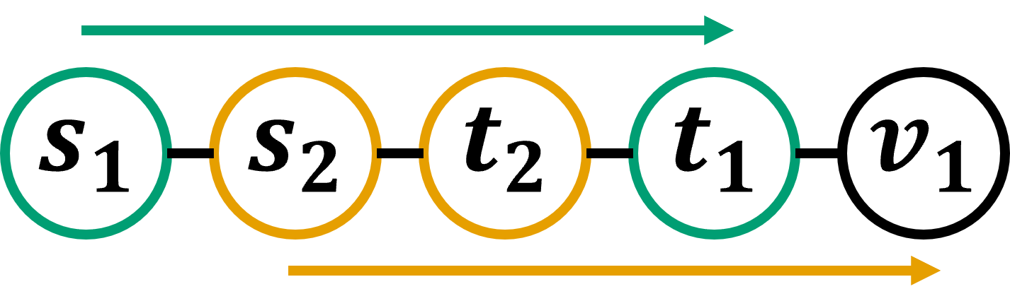
Figure 1: LMAPF problem that cannot be solved as a sequence of MAPF problems.

A significant drawback in this approach stems from the fact that, unlike in MAPF, the agents in LMAPF are not required to reach a configuration where all agents are at their targets, since once an agent reaches its target it may receive a new one. For example, consider the LMAPF problem in Figure 1. Two agents $a_{1}$ and $a_{2}$ are positioned in vertices $s_{1}$ and $s_{2}$ and assigned target $t_{1}$ and $t_{2}$, respectively. As an LMAPF problem, both targets can be reached: once $a_{2}$ reaches its target $t_{2}$ it receives a new target and can choose to move to $v_{1}$ so that $a_{1}$ can also reach its target. Solving this LMAPF problem as a sequence of MAPF problems, however, will fail, because as a MAPF problem, this problem has no solution as the agents cannot swap positions in this graph.

Varambally, Li, and Koenig (2022) and others have acknowledged this MAPF-LMAPF “mismatch” and proposed several techniques to mitigate it to some extent. These techniques include planning for a limited horizon (Li et al. 2021b), dynamic replanning whenever a target is reached (Varambally, Li, and Koenig 2022), defining “dummy paths” to follow after visiting a target  (Liu et al. 2019), and assigning each agent with a sequence of targets (Grenouilleau, Van Hoeve, and Hooker 2019). We discuss these techniques and show they do not provide a complete solution to the MAPF-LMAPF mismatch.

As an alternative, we propose to solve LMAPF problems by solving a sequence of modified MAPF problems that we call Transient MAPF (TMAPF). In TMAPF, the objective is to find conflict-free paths for the agents such that each agent visits its target at some point along its path, but there is no need to reach a configuration in which all agents are at their targets at the same time. We discuss the properties of the TMAPF problem and adapt several popular MAPF algorithms to solve it. Finally, we conduct a small-scale set of experiments comparing the throughput of an LMAPF system when using MAPF and TMAPF algorithms. In some cases, the advantage of using TMAPF algorithms is considerable.

Background

A Multi-Agent Path Finding (MAPF) problem is defined by a graph $G=(V,E)$; a set of agents $A$; and a source and target vertex for each agent $a_{i}\in A$, denoted $s_{i}$ and $t_{i}$, respectively. A solution $\pi$ to a MAPF problem is a mapping of each agent $a_{i}\in A$ to a path $\pi_{i}$ in $G$ such that $\pi_{i}$ starts at $s_{i}$, ends at $t_{i}$, and does not conflict with any path that is mapped in $\pi$ to a different agent. In this work, we consider as a conflict only vertex conflicts and swapping conflicts (Stern et al. 2019). A pair of paths $\pi_{i}$ and $\pi_{j}$ has a vertex conflict if there exists an index $x$ such that $\pi_{i}[x]=\pi_{j}[x]$, where $\pi_{i}[x]$ is the $x^{th}$ vertex in the path $\pi_{i}$. A swapping conflict occurs if there exists an index $x$ such that $\pi_{i}[x]=\pi_{j}[x+1]$ and $\pi_{i}[x+1]=\pi_{j}[x]$. The length of a path is defined as the number of vertices (non-unique) in the path, minus one ($len(\pi_{i})-1$). This version of MAPF is known as Classical MAPF. Sum Of Costs (SOC) and Makespan are common MAPF solution cost function. SOC is the sum of the lengths of all paths in the solution ($\mathit{SOC}(\pi)\coloneqq\sum(len(\pi_{i})-1)|\pi_{i}\in\pi)$) and makespan is the length of the longest path in the solution ($\mathit{Makespan}(\pi)\coloneqq\max(len(\pi_{i})-1|\pi_{i}\in\pi)$). A solution $\pi$ is optimal for a given MAPF problem w.r.t. a given cost function if its cost is smaller than or equal to the cost of any solutions to that MAPF problem. Some MAPF algorithms, such as Conflict Based Search (CBS) (Sharon et al. 2015) guarantee the solution they return is optimal, while others, such as Prioritized Planning (PrP) (Bennewitz, Burgard, and Thrun 2001) do not.

Lifelong Multi-Agent Path Finding (LMAPF) (Li et al. 2021b; Morag, Stern, and Felner 2023) is a generalization of MAPF in which whenever an agent reaches its target, it may be assigned a new target to reach. Due to its online nature, an LMAPF problem is typically solved by repeatedly interleaving planning and execution. In every planning period a path for each agent is computed. Then, a prefix of the planned paths is executed, and another planning period starts. This process continues indefinitely until interrupted by the user. The performance of an LMAPF algorithm is commonly evaluated using throughput, which counts how many times agents reached their targets before a fixed number of time steps have passed. As noted above, a common approach for solving LMAPF is by iteratively calling a MAPF solver every planning period to find paths for the agents from their current locations to their current targets. Different MAPF solvers have been used for this purpose, including optimal and suboptimal MAPF algorithms.

MAPF-LMAPF Mismatch and Mitigations

The role of an LMAPF algorithm is to output plans for the agents in every planning period. We say that an LMAPF algorithm is complete if it does so, and incomplete otherwise. The example in Figure 1 shows that the common approach of solving LMAPF as a sequence of MAPF problems yields incomplete LMAPF algorithms. Several techniques have been proposed for mitigating, to some extent, this incompleteness.

Dynamic replanning

This means whenever a target is reached, all agents immediately replan (Varambally, Li, and Koenig 2022). This option is not feasible in some cases since it requires significant computational cost. Moreover, this approach does not solve the problem in Fig. 1 as the agents will fail to find any MAPF solution.

Pre-assigned sequence of goals

This means each agent is given a sequence of targets to reach and the LMAPF algorithm returns plans to visit the next couple of targets (Grenouilleau, Van Hoeve, and Hooker 2019). Unfortunately, it is not always possible to know such a sequence of tasks for each agent in advance. Also, the planning itself is harder when planning to visit more than one node. Moreover, this technique is also incomplete in some cases.

Dummy paths

This means that after an agent reaches its target, it will follow a pre-defined path so as to avoid causing congestion near its target (Liu et al. 2019). This mitigation strategy still suffers the MAPF limitation that a specific configuration of the agents must be reached. Indeed, identifying effective dummy paths is not trivial and poorly located dummy paths may result in an incompleteness scenario similar to Fig. 1. This technique may also make planning more difficult, as it requires longer paths.

Limited planning horizon

This means ignoring conflicts that are further than $w$ time steps in the future when planning, where $w$ is a parameter. This technique is embodied in the Rolling Horizon Collision Resolution (RHCR) framework (Li et al. 2021b), which is the state of the art in LMAPF. Common implementations of RHCR use LNS (Li et al. 2021a) or PrP for planning, but any MAPF algorithm can be easily adapted for this purpose. While using a limited planning horizon is common, it may lead to deadlocks and to inefficiencies stemming from myopic planning. We show such an example in Fig. 2

Fail policies

Morag et al. (2023) proposed an LMAPF framework designed to handle planning periods in which the underlying MAPF algorithm failed to return a plan. They proposed several fail policies for this purpose and techniques for utilizing partial solutions the MAPF algorithm may return. An LMAPF algorithm with a fail policy can be viewed as a complete LMAPF algorithm, yet the fail policies proposed so far are ad-hoc and may be inefficient.

In summary, while current techniques partially reduce the impact of the MAPF-LMAPF “mismatch”, they do so indirectly and often in an incomplete manner. In this work, we propose a more direct approach to address this mismatch by modifying the type of MAPF problem being solved in every planning period. We call this modified MAPF problem Transient MAPF (TMAPF) and define it below.

A Transient Version of MAPF

The input to a TMAPF problem is the same as the input for MAPF. The solution to a TMAPF problem is also a mapping of each agent to a path in $G$. The key difference between MAPF and TMAPF is that in a solution to a MAPF problem the path $\pi_{i}$ mapped to each agent $a_{i}$ must end at $t_{i}$, in a TMAPF solution it suffices that $\pi_{i}$ includes $t_{i}$. One may view TMAPF as a degenerated version of LMAPF, where when an agent reaches its goal, it is not given a new goal, and use LMAPF algorithms to solve it. As noted above, however, most LMAPF algorithms are not designed to plan paths for agents without a goal, while this is needed for solving TMAPF problems (see Fig. 1).

A notable exception to this is the Priority Inheritance with Backtracking (PIBT) algorithm (Okumura et al. 2022). PIBT was designed to solve Iterative MAPF, which is a generalization of LMAPF in which each agent receives multiple targets to reach. In every iteration PIBT chooses the configuration the agents should move to in the next time step by using a sophisticated version of PrP with a one-step lookahead. Under certain conditions, PIBT guarantees that each agent will reach its target eventually (Okumura et al. 2022).

PIBT is also designed to solve MAPF problems, by continuously re-assigning an agent to its target after it reaches it for the first time, hopefully reaching a configuration where all agents are at their targets simultaneously. PIBT can similarly be adapted to solve TMAPF problems by simply not re-assigning agents to their targets after reaching them, instead associating such agents with a minimal priority hereinafter, allowing other agents to move them if needed.

PrP, LNS, and CBS for Transient MAPF

The one-step lookahead planning done by PIBT often limits its effectiveness in complex scenarios with narrow corridors, which are common in automated warehouses. Instead, many MAPF algorithms such as PrP, LNS, and CBS consider longer planning horizons, using A^∗ (Hart, Nilsson, and Raphael 1968) to find optimal or close to optimal paths in the search-space of locations and time (Erdmann and Lozano-Pérez 1986). To use such algorithms for solving TMAPF problems, we propose to extend the state definition in A^∗ to include a Boolean flag indicating whether or not any of the state’s ancestors visited the agent’s target ($\langle v,x,b\rangle$). This flag is easily maintained by initializing it to $0$ when generating a child state (or the root), and changing it to $1$ if the state contains the target or if the flag was set to $1$ in the parent state ($\mathit{child.b}\leftarrow\mathit{child.v}=t_{i}\vee\mathit{parent.b}$). Extending the state definition is important for two uses. First, two states that have the same time and vertex, but differ in having an ancestor that visited the target, must be considered distinct, and neither must be discarded as a duplicate of the other. Otherwise, the search may miss valid paths. Second, the definition of a goal state is modified to require that the state had an ancestor that visited the target ($\langle v,x,1\rangle$), instead of requiring that the vertex is equal to the target. To differentiate between the MAPF and TMAPF versions we call the MAPF version A^∗, and the TMAPF version A${}^{*}_{t}$.

Experimental Results

We conducted an experimental evaluation of our TMAPF algorithms when solving LMAPF problems on standard grids from the grid-based MAPF benchmark (Stern et al. 2019) and on the pathological cases shown in Fig. 1 and 2. In each experiment, we compare the performance of solving LMAPF problems using either a MAPF or a TMAPF algorithm in every planning period. Specifically, we used PIBT, PrP, CBS, and LNS, and the TMAPF versions of PrP, CBS, and LNS we developed, denoted as PrPt, CBSt, and LNSt. Our LNS implementation only used the Map-Based and Random Destroy Heuristics. All experiments were run on Linux virtual machines in a cluster of AMD EPYC 7763 CPUs, with 16GB of RAM each.

Benchmark Grids

This set of experiments were conducted on grids from the standard MAPF benchmark (Stern et al. 2019). All algorithms were run within the RHCR (Li et al. 2021b) framework. The experiments included LMAPF problems with between 25 and 1000 agents, limited by the maximal number of agents available for each problem in the benchmark. The number of time steps between planning iterations was set to 5, and the planning horizon ($w$) was set to 10, a configuration which was shown to be generally effective in previous works (Li et al. 2021b; Morag, Stern, and Felner 2023). The amount of (real) time for planning at each planning iteration was 5 seconds. The metric we measured was the throughput at time step 1000.

We generated LMAPF instances based on the grid-based MAPF benchmark, generating new targets by selecting locations in the grid randomly (uniformly). Consequently, multiple agents may have the same target at the same time. TMAPF algorithms handle this property organically, while MAPF cannot handle this without planning paths where agents wait until the horizon is exceeded. We run all our experiments within the robust LMAPF framework described by Morag, Stern, and Felner (2023), which includes selecting the agents that should plan in every planning period and determining a fail policy for cases where the planner fails to plan within a given time budget.

In all maps, we observed no significant advantage for using TMAPF, i.e., PrPt exhibited similar results to PrP and LNS exhibited similar results to LNSt. This may be due to the limited planning horizon, which, as mentioned above, can mitigate the effect of the LMAPF-MAPF mismatch. To challenge our algorithms further, we repeated this LMAPF experiments but instead of generating targets randomly from any location in the map, we randomly sampled from a restricted set of 10, 20, 30, or 40 targets. One may argue that these experiments are more realistic than spreading the targets uniformly, especially in real-world applications of LMAPF. For instance, automated warehouses often have fixed picking stations and charging stations that would make certain locations more or less likely to appear as an agent’s target. Similarly, in traffic control, locations such as public transit hubs or office buildings would be common targets for vehicles. Table 1 shows the results of the dense target experiments on maps empty-48-48 and warehouse-20-40-10-2-1. Results on other maps and numbers of agents show similar trends and are available in the supplementary materials. For every map and number of agents, we highlighted in bold the algorithm that achieved the highest throughput between every TMAPF algorithm and its MAPF counterpart. The results show that PrPt and LNSt yield a relatively higher throughput when the number of possible targets is limited. For example, the highest throughput achieved on warehouse-20-40-10-2-1 with 500 agents and 20 targets was 543, achieved by both PrPt and LNSt. For the same map, number of agents, and number of targets, PrP and LNS yielded a throughput of only 491 and 492, respectively. These results highlight the importance of using TMAPF algorithms in such hard and dense LMAPF problems.

Pathological Cases

Next, we evaluated all algorithms on two special LMAPF problems. The first LMAPF problem we consider is based on the example depicted in Fig. 1. Agent $a_{1}$ starts at $s_{1}$ and is assigned targets going back and forth between $s_{1}$ and $t_{1}$, indefinitely. The same is done for agent $a_{2}$ with vertices $s_{2}$ and $t_{2}$. For example, $a_{1}$ will be assigned targets $[t_{1},s_{1},t_{1},s_{1}...]$ . As discussed above, without limiting the planning horizon using a MAPF solver results in planning failure, as the agents must swap their positions, which is impossible. Limiting the planning horizon by using RHCR helps mitigate this problem, which raises the question — is this a substantial problem in LMAPF? We solved this LMAPF problem with a planning horizon of 10, running for 500 time steps, and using PrP, PrPt, and PIBT. We found that PrP and PrPt both achieved a throughput of 500, whereas PIBT achieved a throughput of 320. In comparing A^∗ expansions, PrP required a total of 13,509 expansions, whereas PrPt required only 11,965 expansions. The total runtime was 56ms for PrP, 50ms for PrPt, and 163ms for PIBT. This experiment demonstrates how, even when using RHCR, the new TMAPF solver, PrPt, had advantages in runtime over the MAPF solver PrP, and in throughput over the existing TMAPF solver PIBT.

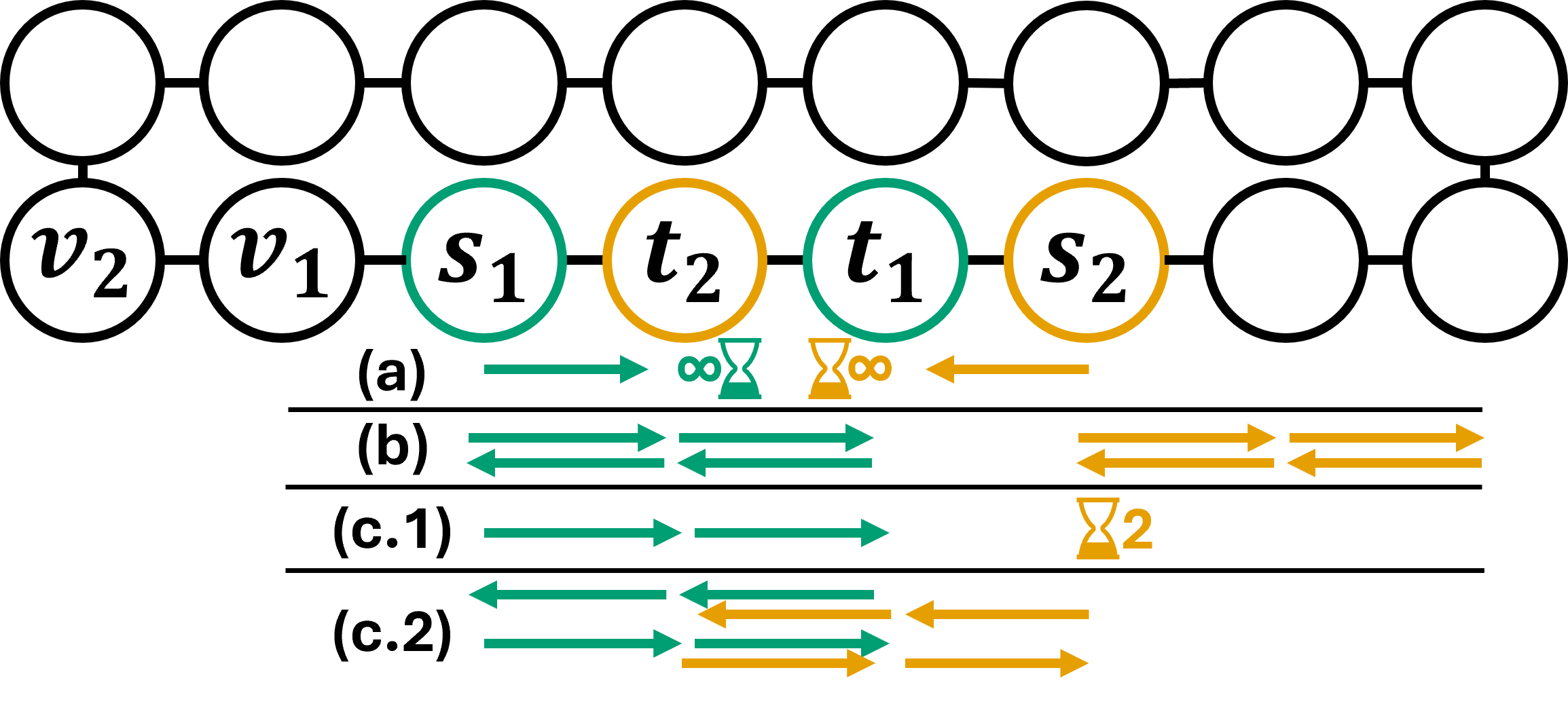
Figure 2: An LMAPF problem in which pathological behaviors occur under different conditions and solvers.

The second special LMAPF problem we consider is illustrated in Figure 2. Here there are two agents, $a_{1}$ and $a_{2}$, tasked with moving repeatedly between $s_{1}$ and $t_{1}$, or $s_{2}$ and $t_{2}$, respectively. All agents are allowed to re-plan at every time step. Consider a planning horizon of $1$ is used. Both the MAPF and TMAPF solvers will behave as seen in Figure 2(a), moving towards each other, and then waiting in place indefinitely, always assuming that once the planning horizon passes they will be able to swap their positions and reach their targets. This results in a throughput of 0 for both solvers. The same would happen with a horizon of $2$ for the TMAPF solver, and any horizon $\leq 5$ for the MAPF solver. Second, assume an infinite planning horizon. The behavior of the MAPF solver is illustrated in Figure 2(b), where it will have $a_{1}$ move counter-clockwise towards its target, while $a_{2}$ attempts to reach its target by moving counter-clockwise. After two time steps, agent $a_{1}$ reaches its target and receives its next target, $s_{1}$. This causes $a_{2}$ to start moving clockwise, to avoid disrupting agent $a_{1}$. This repeats indefinitely, resulting in starvation of agent $a_{2}$, and a throughput of $\mathit{timesteps}\div 2$. This will be true for any horizon larger than $6$. Conversely, the TMAPF solver will have $a_{2}$ wait in place for $a_{1}$ to reach $t_{1}$, as the solver is aware that $a_{1}$ will not be blocking $t_{1}$ indefinitely after reaching it. This is illustrated in Figure 2(c.1). After agent $a_{1}$ reaches $t_{1}$ and receives its new target of $s_{1}$, both agents will start moving clockwise in unison, and reach their new targets after two time steps. They will then move counter-clockwise, and repeat this cycle indefinitely as seen in Figure 2(c.2), resulting in a throughput of $\mathit{timesteps}-1$ . The same will hold true for any horizon larger than $2$. We also studied this behavior experimentally using MAPF and TMAPF versions of CBS and PrP, as well as PIBT. We ran the LMAPF problem for 500 time steps with an infinite planning horizon, and found that the total runtime was 29,198ms for CBS, 33ms for CBSt, 137ms for PrP, 68ms for PrPt, and 80ms for PIBT. Throughput was 250 for CBS, 499 for CBSt, 250 for PrP, 499 for PrPt, and 499 for PIBT. This experiment demonstrates how TMAPF algorithms are useful even while employing existing mitigation for the MAPF-LAMPF mismatch, achieving a higher throughput while requiring less runtime.

		empty-48-48					warehouse-20-40-10-2-1
A	T	LNS	LNSt	PrP	PrPt	PIBT	LNS	LNSt	PrP	PrPt	PIBT
100	10	278	347	427	868	765	115	121	138	141	135
100	20	434	748	632	821	795	123	126	142	143	137
100	30	630	802	744	852	822	129	133	142	143	136
100	40	701	789	783	853	836	129	129	138	138	132
300	10	203	361	205	400	1398	287	314	306	350	362
300	20	505	612	539	1595	2046	363	382	386	408	370
300	30	921	694	1185	2444	2163	394	402	412	421	373
300	40	1106	1011	1560	2457	2239	384	392	402	407	367
500	10	101	217	91	225	1602	338	425	336	432	478
500	20	301	396	317	409	2557	492	543	491	548	515
500	30	414	434	445	495	2997	571	602	585	613	512
500	40	419	441	504	566	3192	615	623	625	637	513

Table 1: Average throughput in our LMAPF dense targets experiment. Columns A and T show the numbers of agents and targets, respectively.

Conclusion and Future Work

In this work, we proposed solving LMAPF problems by solving a sequence of MAPF variants that we call Transient MAPF (TMAPF), in which agents do not have to stay at their targets after visiting them. We described that such a variant is needed to address a mismatch between the requirements of LMAPF and MAPF, and showed how to adapt existing MAPF algorithms to solve it. We evaluated using our TMAPF algorithms within RHCR to solve lifelong MAPF. Our results showed no significant advantage for using TMAPF algorithms when the targets are spread uniformly. However, when the targets are limited to a fixed small number of locations, using the TMAPF algorithms is important, often achieving higher system throughput than their MAPF counterparts. Future work in this line of research may focus on finding ways to select where agents should end their paths in TMAPF to avoid disrupting the other agents. Another direction is to generalize TMAPF to applications where agents must spend some amount of time at their target to complete some task.

Supplementary Materials

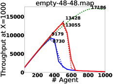
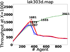
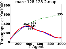
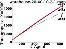
Figure 3: Throughput achieved by the different algorithms as factor of the number of agents.

Figure 3 shows the throughput achieved by the different solvers on different maps within 300 time steps, averaged for each number of agents. The horizontal axis represents the number of agents in the problem instance and the vertical axis represents the throughput. We can see that in all maps the throughput achieved by PrP, PrPt, LNS, and LNSt was similar. PIBT, LaCAM, and LaCAMt also achieved thoughputs that were similar to each other. Which of the two groups had higher throughput depended on the specific map and the number of agents. For example, in maze-128-128-2, the PrP group had higher throughput between 200 and 900 agents, whereas the LaCAM group had higher throughput with 1000 agents.

		empty-48-48					lak303d
# agents	# targets	LNS	LNSt	PrP	PrPt	PIBTt	LNS	LNSt	PrP	PrPt	PIBTt
100	10	279	347	428	868	765	141	149	158	166	153
100	20	434	748	633	822	796	124	126	134	135	125
100	30	631	802	745	852	823	119	121	129	129	119
100	40	701	790	783	854	836	119	119	127	127	118
200	10	265	364	278	491	1238	249	282	279	328	273
200	20	673	785	801	1610	1496	242	244	263	272	237
200	30	1010	1207	1198	1678	1551	235	241	255	258	227
200	40	1102	1465	1334	1678	1589	237	240	254	256	226
300	10	204	361	206	400	1398	337	365	368	445	376
300	20	506	612	540	1595	2047	344	355	380	402	331
300	30	921	694	1185	2445	2164	343	351	377	385	318
300	40	1106	1011	1560	2458	2240	346	348	375	377	315
400	10	138	291	135	314	1513	360	361	365	392	459
400	20	415	481	412	543	2388	413	407	463	451	411
400	30	544	553	670	2371	2665	431	433	480	462	400
400	40	654	572	885	3161	2799	432	442	480	467	395
500	10	102	217	92	225	1603	344	326	344	332	526
500	20	302	396	317	409	2557	437	410	441	434	485
500	30	415	434	446	495	2997	467	452	474	456	471
500	40	420	441	504	567	3192	481	462	488	473	465
		maze-128-128-2					warehouse-20-40-10-2-1
# agents	# targets	LNS	LNSt	PrP	PrPt	PIBTt	LNS	LNSt	PrP	PrPt	PIBTt
100	10	23	23	24	24	22	116	122	139	142	136
100	20	23	23	24	24	22	124	127	142	144	137
100	30	23	23	25	25	23	129	133	143	143	136
100	40	22	22	24	24	22	129	130	138	139	133
200	10	46	47	48	48	42	225	240	253	273	251
200	20	48	48	50	50	45	251	258	274	280	256
200	30	48	48	50	50	45	261	265	281	284	259
200	40	45	45	47	47	42	257	261	273	275	255
300	10	70	69	71	72	62	287	315	307	351	362
300	20	71	71	74	75	63	364	382	387	408	370
300	30	73	73	76	76	65	394	402	413	421	373
300	40	69	68	71	72	61	385	392	402	407	367
400	10	92	93	94	95	80	313	376	322	388	465
400	20	94	95	97	97	82	438	476	454	491	476
400	30	95	96	99	99	83	501	517	515	538	478
400	40	91	90	94	94	80	506	515	524	532	471
500	10	112	113	115	115	94	338	426	336	433	566
500	20	115	116	120	120	100	492	543	491	549	579
500	30	118	118	120	120	101	572	603	586	614	576
500	40	109	110	111	112	95	615	632	626	637	572

Table 2: Throughput achieved by different algorithms in our LMAPF dense targets experiment, averaged over 25 instances.

Table 2 shows the full results of the dense target experiments on maps empty-48-48, warehouse-20-40-10-2-1, maze-128-128-2, and lak303d. For every map and number of agents, we highlighted in bold the algorithm that achieved the highest throughput between every TMAPF algorithm and its MAPF counterpart. The results show that the TMAPF algorithms have a significant advantage in terms of throughput when the number of possible targets is limited. For example, the highest throughput achieved on warehouse-20-40-10-2-1 with 500 agents and 30 targets was 594, achieved by LNSt and PrPt. For the same map, a number of agents, and a number of targets, LNS and PrP yielded a throughput of only 361 and 352, respectively

References

- Bennewitz, Burgard, and Thrun (2001) Bennewitz, M.; Burgard, W.; and Thrun, S. 2001. Optimizing schedules for prioritized path planning of multi-robot systems. In IEEE International Conference on Robotics and Automation (ICRA), volume 1, 271–276.
- Erdmann and Lozano-Pérez (1986) Erdmann, M. A.; and Lozano-Pérez, T. 1986. On multiple moving objects. In Proceedings of the 1986 IEEE International Conference on Robotics and Automation, San Francisco, California, USA, April 7-10, 1986, 1419–1424. IEEE.
- Felner et al. (2017) Felner, A.; Stern, R.; Shimony, S.; Boyarski, E.; Goldenberg, M.; Sharon, G.; Sturtevant, N.; Wagner, G.; and Surynek, P. 2017. Search-based optimal solvers for the multi-agent pathfinding problem: Summary and challenges. In Proceedings of the International Symposium on Combinatorial Search, volume 8, 29–37.
- Grenouilleau, Van Hoeve, and Hooker (2019) Grenouilleau, F.; Van Hoeve, W.-J.; and Hooker, J. N. 2019. A multi-label A* algorithm for multi-agent pathfinding. In International conference on automated planning and scheduling, 181–185.
- Hart, Nilsson, and Raphael (1968) Hart, P. E.; Nilsson, N. J.; and Raphael, B. 1968. A formal basis for the heuristic determination of minimum cost paths. IEEE transactions on Systems Science and Cybernetics, 4(2): 100–107.
- Li et al. (2021a) Li, J.; Chen, Z.; Harabor, D.; Stuckey, P.; and Koenig, S. 2021a. Anytime multi-agent path finding via large neighborhood search. In Proceedings of the International Joint Conference on Artificial Intelligence (IJCAI).
- Li et al. (2021b) Li, J.; Tinka, A.; Kiesel, S.; Durham, J. W.; Kumar, T. S.; and Koenig, S. 2021b. Lifelong multi-agent path finding in large-scale warehouses. In Proceedings of the AAAI Conference on Artificial Intelligence, volume 35, 11272–11281.
- Liu et al. (2019) Liu, M.; Ma, H.; Li, J.; and Koenig, S. 2019. Task and path planning for multi-agent pickup and delivery. In Proceedings of the International Joint Conference on Autonomous Agents and Multiagent Systems (AAMAS).
- Ma et al. (2017) Ma, H.; Li, J.; Kumar, T.; and Koenig, S. 2017. Lifelong Multi-Agent Path Finding for Online Pickup and Delivery Tasks. In International Conference on Autonomous Agents and Multiagent Systems.
- Morag, Stern, and Felner (2023) Morag, J.; Stern, R.; and Felner, A. 2023. Adapting to Planning Failures in Lifelong Multi-Agent Path Finding. In Proceedings of the International Symposium on Combinatorial Search, volume 16, 47–55.
- Okumura et al. (2022) Okumura, K.; Machida, M.; Défago, X.; and Tamura, Y. 2022. Priority inheritance with backtracking for iterative multi-agent path finding. Artificial Intelligence, 310: 103752.
- Sharon et al. (2015) Sharon, G.; Stern, R.; Felner, A.; and Sturtevant, N. R. 2015. Conflict-based search for optimal multi-agent pathfinding. Artificial intelligence, 219: 40–66.
- Stern et al. (2019) Stern, R.; Sturtevant, N. R.; Felner, A.; Koenig, S.; Ma, H.; Walker, T. T.; Li, J.; Atzmon, D.; Cohen, L.; Kumar, T. S.; et al. 2019. Multi-agent pathfinding: Definitions, variants, and benchmarks. In Symposium on Combinatorial Search (SoCS).
- Švancara et al. (2019) Švancara, J.; Vlk, M.; Stern, R.; Atzmon, D.; and Barták, R. 2019. Online multi-agent pathfinding. In AAAI conference on artificial intelligence, volume 33, 7732–7739.