Multipartite entanglement distribution in Bell-pair networks
without Steiner trees and with reduced gate cost

Abstract

Multipartite entangled states, particularly Greenberger–Horne–Zeilinger (GHZ) and other graph states, are important resources in multiparty quantum network protocols and measurement-based quantum computing. We consider the problem of generating such states from networks of bipartite entangled (Bell) pairs. Although an optimal protocol (in terms of time steps and consumed Bell pairs) for generating GHZ states in Bell-pair networks has been identified in [Phys. Rev. A 100, 052333 (2019)], it makes use of at most $O(N^{2})$ gates, where $N$ is the number of nodes in the network. It also involves solving the NP-hard Steiner tree problem as an initial step. Reducing the gate cost is an important consideration now and into the future, because both qubits and gate operations are noisy. To this end, we present a protocol for producing GHZ states in arbitrary Bell-pair networks that provably requires only $O(N)$ gates, and we present numerical evidence that our protocol indeed reduces the gate cost on real-world network models, compared to prior work. Notably, the gate cost of our protocol depends only on the number of nodes and is independent of the topology of the network. At the same time, our protocol maintains nearly the optimal number of consumed Bell pairs, and it avoids finding a Steiner tree or solving any other computationally hard problem by running in polynomial time with respect to $N$. By considering the number of gates as a figure of merit, our work approaches entanglement distribution from the perspective that, in practice, unlike the traditional information-theoretic setting, local operations and classical communications are not free.

I Introduction

Recent years have seen a rapid rise in the development and realization of small-scale quantum devices, such as small-scale quantum computers and quantum sensors [1, 2, 3, 4]. Individually, these small-scale devices are not particularly powerful nor useful. However, by networking these small-scale devices, it may become possible to execute large-scale applications in a distributed fashion [5, 6, 7], and thus make strides towards the goal of quantum advantage.

Entanglement is the resource that enables distributed quantum information processing tasks, such as quantum communication, computation, and sensing, over long distances. Both bipartite and multipartite entanglement can be used to achieve these tasks. Indeed, bipartite entanglement, along with local operations and classical communication (LOCC) between spatially separated nodes, enables the fundamental protocol of teleportation [8, 9], and multipartite entanglement enables various distributed and measurement-based quantum computing strategies [10, 11, 12, 13, 14, 15, 16, 17, 18, 19], and can enhance quantum sensing [20, 21, 22, 23, 24].

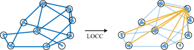
Figure 1: (Top) A network of Bell pairs, consisting of nodes (black circles) containing qubits (blue circles). Every edge connecting two qubits represents a Bell pair. Our goal is to transform the Bell-pair network, via local operations and classical communication (LOCC), to a graph state. (Bottom) A star graph state (which is local-unitary-equivalent to a GHZ state) shared by all nodes in the network.

The creation of bipartite entanglement (e.g., Bell pairs) between nearest neighbors in a network has been realized experimentally in recent years [25, 26, 27, 28, 29, 30, 31, 32, 33, 34, 35], and will arguably form the backbone of large-scale quantum networks. Therefore, when considering the distribution of multipartite entanglement in quantum networks, it is meaningful to consider protocols in which the aim is to transform a network of Bell pairs, via LOCC, into a multipartite entangled state shared by a given set of nodes in the network; see Fig. 1. Some prior works assume that these multipartite entangled states are already distributed in advance in the network [36, 37, 38, 39], without consideration of how this might be done in the first place. Other works consider first creating the multipartite states locally, and then distributing them over quantum channels and/or via teleportation [40, 41, 42, 43] using the network of nearest-neighbor Bell pairs. The latter strategy requires quantum repeater protocols [44, 45, 46, 47, 48] for creating Bell pairs between one node and all of the others.

In this work, we consider LOCC-based entanglement distribution of multipartite entangled states directly from a network of Bell pairs, as illustrated in Fig. 1. Previously, Ref. [40] has provided a protocol in this setting that creates a graph state shared among all nodes in the network, such that the topology of the corresponding graph mimics that of the Bell-pair network. They have shown that their protocol can outperform the repeater-based protocol that first creates bipartite entanglement between one node and all of the others and then teleports the locally-created graph state. Similarly, Ref. [49] provides a protocol for distributing an arbitrary graph state using a network of Bell pairs, even among a chosen subset of nodes, but this protocol involves (in the most general case) solving the NP-hard Steiner tree problem [50, 51] as an initial step. The protocol in Ref. [42] involves generating the graph state locally at a node and then distributing the state to the other nodes via appropriately selected paths using the Bell-pair network. We refer to App. A for a more detailed summary of prior work.

The main contribution of our work is an alternative protocol for distributing graph states, specifically Greenberger–Horne–Zeilinger (GHZ) states [52], in arbitrary network topologies directly from the Bell pairs that connect the nearest-neighbor nodes of the network. Our protocol is based on successively creating small GHZ states, starting from the highest-degree nodes, and then merging them to obtain larger GHZ states that eventually span either the entire network or some given subset of nodes. Unlike Ref. [49], our protocol is not based on solving the Steiner tree problem, nor any other computationally hard problem. Also, unlike Ref. [42], our protocol does not require first creating Bell pairs between one node in the network and all of the others. Nevertheless, we can provably achieve either comparable or better performance compared to Refs. [49, 42] for the figures of merit that we consider.

The usual figures of merit for assessing the performance of entanglement distribution protocols include the number of Bell pairs used, waiting time, and fidelity. In this work, we consider an additional figure of merit: the total number of (local) gates used. This additional figure of merit is motivated by the fact that, currently, qubits and gates are prone to errors, and should therefore not be considered free. This is in contrast to the usual information-theoretic setting of entanglement distribution, in which LOCC operations are considered free. Accordingly, LOCC operations are considered free in Refs. [49, 42]. Instead, we advocate the message that entanglement distribution protocols should aim to minimize the number of gates, in addition to optimizing the other figures of merit, and we ask the question:

How many gates are needed to distribute a multipartite entangled state within a Bell-pair network?

We present our protocol in Sec. II. Then, in Sec. III, we present our first result, addressing the above question, which is that our protocol requires $O(N)$ gates to produce a GHZ state shared by all nodes in the network; see Sec. III.1. On the other hand, we prove that the protocol of Ref. [49] requires at most $O(N^{2})$ gates, and in Sec. IV we provide numerical evidence that our protocol indeed improves the gate count compared to Ref. [49]. It is also remarkable that the gate count for our protocol depends only on the number $N$ of nodes, and not on any other property of the network, e.g., topology and density of nodes.

We also prove that our protocol consumes the same optimal number of Bell pairs as in Ref. [49] when entangling all nodes in the network (see Sec. III.2), and in Sec. IV we provide numerical evidence that our protocol is nearly optimal with respect to consumed Bell pairs when entangling a subset of nodes, i.e., the number of consumed Bell pairs in our protocol is close to that of the Steiner tree approach of Ref. [49].

Our protocol has several notable features. By creating the small-scale GHZ states independently, our protocol is less susceptible to the failure of any single GHZ state creation, which might result from the failure of nearest-neighbor entanglement generation in networks of lossy optical fiber channels. In cases of failure, the other GHZ states can be stored in memory, potentially reducing overall waiting times. Additionally, by creating small-scale GHZ states at the highest-degree nodes within the network, our protocol minimizes the required number of Bell pair sources. These sources only need to be located at the highest-degree nodes, rather than at every individual node. Finally, we prove that our protocol runs in polynomial time with respect to the number of nodes in the network.

In Sec. IV, we assess the performance of our protocol on models of real networks, which often exhibit the small-world property, along with high density and central hubs. We consider the Erdős–Rényi, Barabási–Albert, and Waxman models [53, 54, 55, 56, 57, 58, 59, 60], which capture these realistic network features. Our protocol, by focusing on creating local GHZ states at the highest-degree nodes, is inherently well suited to these realistic network models. Accordingly, we find that the gate cost of our protocol, as stated above, is independent of the model parameters of these network models, depending only on the number of nodes and not on the topology nor the density. In contrast, we find rather counterintuitively that the gate cost for the protocol of Ref. [49] increases with network density. Finally, in Sec. V, we consider our protocol in the presence of noise, both noisy gates and noisy Bell pairs, and we derive exact analytical expressions for the fidelity of the output state with respect to the desired GHZ state. These analytical expressions hold for arbitrary noise models for both the Bell pairs and the gates.

II Our protocol

We model a network with a graph. The vertices of the graph correspond to the nodes in the network. Every node has a number of qubits equal at least to the degree of the corresponding vertex. The edges in the graph dictate how these qubits within the nodes are connected to the qubits in other nodes via quantum channels, which are used to generate Bell pairs $|\Phi\rangle\coloneqq\frac{1}{\sqrt{2}}(|0,0\rangle+|1,1\rangle)$ between the qubits in different nodes. In particular, if the graph has a vertex with degree $k$, then its corresponding network has a node with $k$ qubits, and each one of these qubits can be connected via a Bell pair to a qubit in the neighboring node; see Fig. 1 for an example. Starting from the network of Bell pairs, we consider the task of distributing a GHZ state among either all nodes of the network (the complete case) or a given subset of nodes in the network (the subset case). Every qubit of the GHZ state should belong to one of the desired nodes in the network.

The $N$-party GHZ state is defined as [52] $|\text{GHZ}_{N}\rangle\coloneqq\frac{1}{\sqrt{2}}(|0\rangle^{\otimes N}+|1\rangle^{\otimes N})$. GHZ states are useful, for instance, for conference key agreement [61], and are necessary for achieving optimal precision in certain quantum metrological tasks [20, 21]. Graphically, GHZ states can be depicted using a star graph; see Fig. 2. Notably, because the GHZ state is permutation invariant, the center of the star can be placed at any of the qubits, a fact that we make use of extensively in our protocol. (This fact is in contrast to the star graph state, which has a distinguished central qubit, and to change the central qubit requires local operations; see App. B.) Throughout the rest of this work, we use the term “star” to refer to both a GHZ state and its graphical depiction.

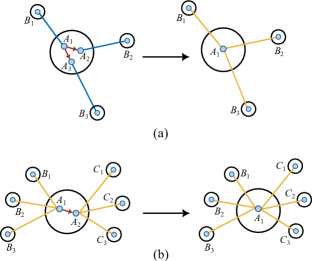
Figure 2: (a) Creation of a GHZ state using Bell pairs connected to a central node (Protocol 2). Arrows indicate CNOT gates, pointing from source qubits to target qubits. (b) Merging of two GHZ states to create a larger GHZ state (Protocol 3). In both protocols, after the CNOT gates, the target qubits are measured in the Pauli-$Z$ basis.

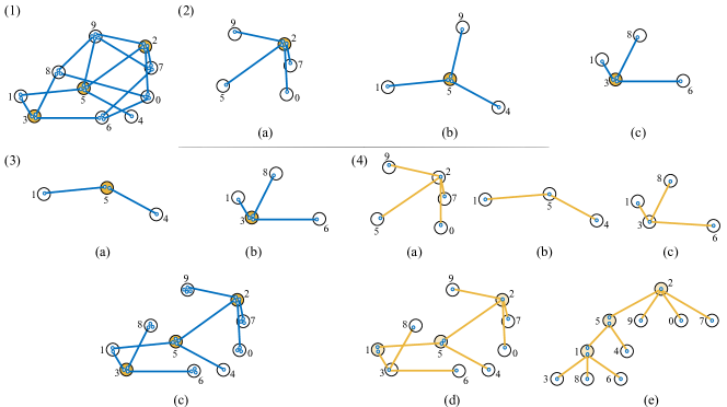
Figure 3: An example of using Protocol 1 to distribute a GHZ among all nodes of a network. (1) The initial network of Bell pairs, with the nodes chosen in Steps 1–3 highlighted. (2) The highest degree nodes chosen in Steps 2–4 and the corresponding star subgraphs. The corresponding stars comprise the list SG. (a) The node 2 has the highest degree in the initial network. (b) After removing node 2 from the network, node 5 has the highest degree. (c) After removing node 5, node 3 has the highest degree. At this point, all nodes are accounted for. (3) Iterations of Steps 6–11. The star S0 is the one in (2a). The list MSG contains S0, S1, S2, where S1 is in (3a) and S2 is in (3b). In (3c), the initial network is shown with only those edges corresponding to the stars in MSG. (4a–c) The result of Step 12. In (4d), the initial network is shown with the locally-created GHZ states from Step 12, and in (4e) these GHZ states are arranged explicitly into a tree, after placing the center of the star in (4c) at node 1.

In Protocol 1, we present our protocol for creating a GHZ state in an arbitrary network of Bell pairs. The protocol comprises two main components, illustrated in Fig. 2: Protocol 2, which creates local, small-scale GHZ states centered around nodes with the highest degree; and Protocol 3, which merges these small-scale GHZ states to achieve the desired GHZ state among all of the desired nodes. We refer to App. D for details on Protocol 2 and App. E for details on Protocol 3. In App. E, we also provide a generalization of Protocol 3 to the merging of more than two GHZ states. In Fig. 3, we provide an example of how Protocol 1 works.

In the subset case, we can first generate a GHZ state for the entire graph using our Protocol 1 and then use $X$-measurements to remove the qubits outside of the target subset, resulting in a GHZ state shared among the desired nodes. However, this method consumes significantly more gates and Bell pairs than necessary. Instead, we first apply Protocol 4, which constructs a connected subgraph that includes the desired nodes, then we generate the GHZ state within this subgraph using Protocol 1, and finally we $X$-measure out any qubits in the subgraph that are not part of the target subset. (If the set of desired nodes already forms a connected subgraph, then Protocol 4 is not required.) We provide an example of how Protocol 4 works in Fig. 4. Note that this initial step of constructing a connected subgraph is in contrast to the protocol in Ref. [49]—which we refer to as the “MMG protocol” from now on—in which the subset case involves first identifying a Steiner tree (a process known to be NP-hard [62]) and then executing the star expansion protocol of the same work to obtain the GHZ state among the selected nodes. In our case, we need not produce a tree, and indeed Protocol 4 will not necessarily produce a tree subgraph.

Protocol 1 GHZ creation in a Bell-pair network

1:Network of Bell pairs, represented by a graph $G$ with $N$ nodes.

2:GHZ state shared among all $N$ nodes.

3:Create an empty list, SG.

4:Identify the node in $G$ with the highest degree. If there are multiple, select one at random.

5:Save the star subgraph, consisting of the selected node and its neighboring nodes, as an element in SG.

6:Remove the selected node and its associated edges from $G$.

7:Repeat steps 2–4 until all nodes in $G$ are included in at least one star.

8:Add all remaining edges from $G$, along with their two associated nodes, as elements in SG.

9:Select the largest star in SG, label it S0, and remove it from SG.

10:Create a new list called MSG and add S0 to it.

11:Find another star in SG that shares at least one node in common with any star in MSG and call it S1.

12:Check if all nodes of S1 are already in any stars of MSG. If so, remove S1 from SG and return to the previous step.

13:If the center node of S1 is in common with any star in MSG, remove all common nodes (and the associated edges) from S1 except its center node. If not, remove all common nodes (and the associated edges) except one randomly-chosen common node. Remove S1 from SG and add the modified S1 to MSG.

14:Repeat steps 8–10, naming stars as S2, S3, etc., until SG is empty.

15:For every star in MSG, apply Protocol 2 to create a GHZ state among the nodes in the star.

16:Merge S0 with S1 at their common node using Protocol 3. Then merge the resulting star with S2 at their common node, repeating until all stars are merged into one.

Protocol 2 GHZ state from Bell pairs in a star topology

1:$n\in\{2,3,\dotsc\}$ Bell pairs $|\Phi\rangle_{A_{i}B_{i}}$, $N=n+1$ nodes in a star topology. (The central node shares a Bell pair with each of the $n$ outer nodes.)

2:GHZ state $|\text{GHZ}_{N}\rangle$ shared by all $N$ nodes.

3:Apply the CNOT gates $\text{CNOT}_{A_{1}A_{2}}$, $\text{CNOT}_{A_{1}A_{3}}$, …,$\text{CNOT}_{A_{1}A_{n}}$ on the qubits in the central node.

4:Measure the qubits $A_{2},A_{3},\dotsc,A_{n}$ in the $Z$-basis $\{|0\rangle,|1\rangle\}$.

5:Communicate the outcome of the measurement on qubit $A_{i}$ to the qubit $B_{i}$, $i\in\{2,3,\dotsc,n\}$. For every $i\in\{2,3,\dotsc,n\}$: if the outcome communicated by $A_{i}$ is 0, then nothing is done on qubit $B_{i}$; if the outcome communicated by $A_{i}$ is 1, then apply the Pauli-$X$ gate to qubit $B_{i}$.

Protocol 3 Merging two GHZ states

1:Two GHZ states, $|\text{GHZ}_{n+1}\rangle_{A_{1}B_{1:n}}$ and $|\text{GHZ}_{m+1}\rangle_{A_{2}C_{1:m}}$, $n,m\in\{1,2,\dotsc\}$, such that qubits $A_{1}$ and $A_{2}$ are located at the same node.

2:GHZ state $|\text{GHZ}_{n+m+1}\rangle_{A_{1}B_{1:n}C_{1:m}}$.

3:Perform the gate $\text{CNOT}_{A_{1}A_{2}}$ between the qubits $A_{1}$ and $A_{2}$.

4:Measure the qubit $A_{2}$ in the $Z$-basis (i.e., the $\{|0\rangle,|1\rangle\}$ basis).

5:Communicate the outcome $x\in\{0,1\}$ of the measurement to the nodes $C_{1},C_{2},\dotsc,C_{m}$. If the outcome is $x=0$, then $C_{1},C_{2},\dotsc,C_{m}$ do nothing; if the outcome is $x=1$, then $C_{1},C_{2},\dotsc,C_{m}$ apply the Pauli-$X$ gate to their qubits.

Protocol 4 Connected subgraph generation

1:Network of Bell pairs, represented by a graph $G$ with $N$ nodes, and a list of desired nodes, DN.

2:A connected subgraph of $G$ containing all of the nodes in DN.

3:Generate the subgraph induced by DN, call it $G^{\prime}$. This subgraph may not be connected; if it is connected, output $G^{\prime}$.

4:Randomly choose a node from DN to serve as the root node. Using a breadth-first search (BFS) algorithm [63], create a tree-like structure starting from the root node by visiting its first-level neighbors, then the second-level neighbors, and so on, without repeating any nodes (see Fig. 4).

5:Iteratively delete leaf nodes (red nodes in Fig. 4) from the BFS tree unless they are part of the desired nodes (DN). Continue this process until all remaining leaf nodes belong to DN, and no further removals are possible.

6:Construct a subgraph using nodes from BFS tree (yellow and blue nodes from Fig. 4) and corresponding edges from $G$.

Figure 4: An example of using Protocol 4 to determine a connected subgraph containing a desired subset of nodes. (a) The original network, with the desired nodes highlighted in yellow, forming the set $\texttt{DN}=\{0,1,6,9\}$. (b) The nodes highlighted in red are not necessary and can be deleted, while the nodes highlighted in blue are necessary to have a connected subgraph. The resulting subgraph $G$ consists of the desired yellow nodes and the blue nodes.

Remarks

1. The graph $G$ in Protocol 1 can be arbitrary, as long as it is connected. Indeed, because we are in the LOCC setting, an LOCC protocol can create a GHZ among all nodes of $G$ only if $G$ is connected, i.e., if there exists a path connecting every pairs of vertices in $G$.

2. The input graph to Protocol 1 can be a minimal spanning or Steiner tree corresponding to a given graph and a set of desired nodes to be entangled. However, unlike the MMG protocol [49], we emphasize that finding such a tree is not required as an initial step.

3. Our protocols operate with polynomial time complexity, as we prove below in Theorem 7 and Theorem 8.

4. In our protocols, the locations of the star creations are not unique, in part because the highest-degree nodes (selected in Step 2 of the protocol) need not be unique and are chosen randomly. For the example in Fig. 3, panels (1) and (2), the algorithm determines that we create local GHZ states at nodes 2, 5, and 3; from panel (4), we see that the merges should occur at nodes 9 and 1.

5. Protocol 1 requires a number of Bell pairs equal to the total sum of Bell pairs across all the stars in the list MSG from step 12. Merging stars does not require any additional Bell pairs, and the number of Bell pair sources corresponds to the number of elements in the list MSG.

6. Our protocols determine where the small-scale GHZ states should be created and how they should be merged, and they do so in an offline manner. Furthermore, Protocol 1 will produce a tree structure. Importantly, this is not just any tree; it will feature a specific root structure aimed at minimizing the number of Bell pair sources required for the process.

7. If the given network has one node with a degree equal to $N-1$—that is, a node connected to all other nodes—then the protocol finishes in one step.

III Analytical results

The number of Bell pairs and the total number of gates used are the two figures of merit considered in the analytical analysis of the above algorithm. It is assumed that all gates have equal and unit efficiencies, and that the Bell pairs are distributed without losses and with unit fidelity. The analysis of our protocol in the presence of losses is discussed in Sec. V, while the numerical results are presented in Sec. IV.

III.1 Gate cost

To determine the gate cost of our protocol, we start by counting the number of gates needed in Protocols 2 and 3.

1. Protocol 2 requires $n-1=N-2$ gates, where $n$ is the number of Bell pairs input to the protocol and $N=n+1$ is the number of nodes involved in the protocol.

2. Protocol 3 requires one gate, independent of the sizes of the GHZ states being merged.

Note that we do not consider the Pauli correction gates in the gate count.

Theorem 1 (Number of gates: complete case).

The gate cost of Protocol 1 in the complete case is $N-2$ gates, where $N$ is the total number of nodes in the network.

Proof.

Let us assume there are a total of $N$ nodes and these are distributed in $k$ GHZ states of different sizes. The number of nodes in each GHZ state is given by $n_{1},n_{2},n_{3},\dotsc,n_{k}$. The number of gates required to create these GHZ states is given by (according to point 1 above) $(n_{1}-2),(n_{2}-2),(n_{3}-2),\dotsc,(n_{k}-2)$. Adding up all of these gives us $n_{1}+n_{2}+n_{3}+\dotsb+n_{k}-2k$. As there are $k$ GHZ states, there will be $k-1$ nodes that are repeated one time. Therefore, the total number of nodes in all of the small GHZ states should be $N+k-1$, i.e., $n_{1}+n_{2}+n_{3}+\dotsb+n_{k}=N+k-1$, which means that the gate cost is $N+k-1-2k=N-k-1$. Now, let us add the gates for the merging of the GHZ states (explained in point 2 above). As there are $k$ GHZ states, there will be $k-1$ merges in total, and each merge requires one gate (see point 2 above), which means that the total number of gates required is $N-k-1+k-1=N-2$.  $\blacksquare$

Theorem 2 (Number of gates: subset case).

In the subset case, the gate cost of our protocol is $S-2$ gates where $S$ is the total number of nodes in the subgraph (the subgraph obtained using Protocol 4).

Proof.

The proof is analogous to the proof of Theorem 1.  $\blacksquare$

It is notable here that the number of gates depends only on the number of nodes in the subgraph—no specific properties of the structure/topology/connectivity of the graph matters, except for the fact that it should be connected. In particular, this means that if we take any fraction $f\in(0,1]$ of the nodes $N$ of our network to comprise our subset, then the size $S$ of the subgraph containing these nodes satisfies $S\geq Nf$, which means that the number of gates is bounded from below as $S-2\geq Nf-2$.

Comparison to Ref. [49].

The gate cost of the star expansion protocol of Ref. [49] is as follows. If $k$ is the degree of the node on which the star expansion protocol is performed, then:

• If the central node is to be kept, then the number of gates is $g_{1}(k)\coloneqq\binom{k}{2}+2k-1=\frac{1}{2}k^{2}+\frac{3}{2}k-1$.

• If the central node is to be discarded, then the number of gates is $g_{2}(k)\coloneqq\binom{k}{2}+k=\frac{1}{2}k^{2}+\frac{1}{2}k$.

Using this, we can establish the following fact about the number of gates required to create a GHZ state according to the protocol in Ref. [49].

Proposition 3 (Upper bound on gate cost of the MMG protocol [49]).

For any graph with $N$ nodes, the number of gates required to create a GHZ state among all $N$ nodes, according to the MMG protocol, scales as $O(N^{2})$.

Proof.

The MMG protocol of Ref. [49] proceeds by starting with a minimal spanning tree for the graph. Then, an arbitrary leaf node of the tree is chosen, and the star expansion protocol is applied successively on non-leaf neighbors of the chosen leaf node until all of the nodes are included in the GHZ state. If the number of non-leaf neighbors is $L$, then the gate cost is $\sum_{i=1}^{L}g_{1}(k_{i})$. We can bound this from above by summing over all nodes, i.e.,

$$\sum_{i=1}^{L}g_{1}(k_{i}) \leq\sum_{i=1}^{N}g_{1}(k_{i})$$ (1)

$$=\frac{1}{2}\sum_{i=1}^{N}k_{i}^{2}+\frac{3}{2}\sum_{i=1}^{N}k_{i}-N$$ (2)

$$\leq\frac{1}{2}\left(\sum_{i=1}^{N}k_{i}\right)^{2}+\frac{3}{2}\cdot 2(N-1)-N$$ (3)

$$=\frac{1}{2}(2(N-1))^{2}+2N-3$$ (4)

$$=2N^{2}-2N-1$$ (5)

$$=O(N^{2}),$$ (6)

where we have made use of the fact that $\sum_{i=1}^{N}k_{i}=2(N-1)$, i.e., the sum of the degrees is equal to twice the number of edges, and the number of edges in the minimal spanning tree is necessarily $N-1$.  $\blacksquare$

Let us now also observe that we can significantly reduce the gate cost of the star expansion Protocol by noticing that the end result of the protocol is a GHZ state, either with or without the central node. If the central node is to be excluded, then by the Bipartite B protocol (see App. C), the gate cost is $k-1$. If the central node is to be included, then the gate cost is also $k-1$, using the protocol in App. D. This represents a quadratic reduction in gate cost, from $O(k^{2})$ (as established in Ref. [49]) to $O(k)$.

Comparison to Ref. [42].

The lower bound on gate count in [42] is reached when a single node is connected to all other nodes in the graph, resulting in $N-2$ gates—consistent with our protocol’s gate count. However, as we prove below, the upper bound in [42] scales as $O(N^{2})$. Therefore, our protocol generally achieves a lower gate count, except in the specific scenario where one node connects to all others, in which case our protocol matches the gate count in [42].

Proposition 4 (Upper bound on gate cost in Ref. [42]).

For a graph with $N$ nodes, the upper bound on the number of gates required to create a GHZ state across all $N$ nodes, as specified by the protocol in Ref. [42], scales as $O(N^{2})$.

Proof.

Consider a chain topology for the network, with nodes labeled from 1 to $N$ from left to right. Suppose that the root node is node 1. In this setup, the protocol of Ref. [42] requires “connection transfers” from each node to node 1, with each transfer utilizing one gate. The farthest node, node $N$, requires $N-2$ connection transfers to reach node 1. The next farthest node, node $N-1$, requires $N-3$ connection transfers, and so on. Consequently, the total number of gates used is given by $(N-2)+(N-3)+(N-4)+\dotsb+(N-N)=\sum_{j=2}^{N}(N-j)=\frac{N(N-3)}{2}+1=O(N^{2})$.  $\blacksquare$

III.2 Bell pair cost

Theorem 5 (Number of Bell pairs used: complete case).

For the complete case of our protocol, the number of Bell pairs used is equal to $N-1$. This matches the lower bound of $N-1$, which is the minimum number of Bell pairs needed to create an arbitrary graph state.

Proof.

The proof consists of two parts. First, we establish that the lower bound is $N-1$; second, we show that our protocol achieves this bound.

To begin, the network must be connected, as it is otherwise impossible to generate entanglement among all nodes in the LOCC setting. The minimum number of edges required to connect a graph of $N$ nodes is $N-1$, which implies that at least $N-1$ Bell pairs are needed. This gives us the lower bound of $N-1$ Bell pairs.

To minimize the number of Bell pairs, a single common node between any two stars is necessary and sufficient for merging. If more than one common node is present, additional Bell pairs are consumed. Therefore, in step 10 of our protocol, we modify the stars to ensure that only one common node connects with the rest. This ensures that we require only $N-1$ Bell pairs to create the GHZ state.  $\blacksquare$

Let us now examine the number of Bell pairs in the subset case by introducing the concept of the graph diameter. The diameter of an unweighted graph is defined as the length of the longest shortest path between any two nodes. In simpler terms, it is the greatest distance, measured by the number of edges, between any pair of nodes. Here, the shortest path refers to the path connecting two nodes with the fewest edges.

Theorem 6 (Number of Bell pairs used: subset case).

Let $S$ be the size of the connected subgraph containing the desired subset of nodes, as generated from Protocol 4. The number of Bell pairs needed to generate a GHZ state is bounded from below by $S-1$ and bounded from above by $d_{S}(S-1)$, where $d_{S}$ is the diameter of the connected subgraph containing the desired subset of nodes, as generated from Protocol 4.

Proof.

For the lower bound, the minimum number of Bell pairs used is determined analogous to the complete case, resulting in $S-1$.

For the upper bound, the maximum number of Bell pairs will be used when all the nodes in the subset are maximally distant from each other. By definition, the diameter gives the maximum distance in terms of the number of Bell pairs. Since there are $S$ maximally distant nodes, the maximum number of Bell pairs used is $d_{S}(S-1)$.  $\blacksquare$

Comparison to Refs. [49, 42].

In the complete case, for the MMG protocol [49], the number of Bell pairs required is $N-1$, as it corresponds to the size of the minimal spanning tree. This is the same number of Bell pairs used in our protocol (Theorem 5). However, the approach in Ref. [42] requires additional Bell pairs to connect the desired node to every other node, unlike our protocol and the MMG protocol. In the subset case, the number of Bell pairs needed in the MMG protocol is equal to the size of the tree, which will generally exceed $N_{s}-1$, where $N_{s}$ is the number of nodes in the subset. This is because the Steiner tree will typically include more nodes than just the terminal nodes. In Ref. [42], the same logic applies as in the complete case.

III.3 Time complexity

We now present results on the time complexity of our protocols in the worst-case scenario, focusing solely on the classical steps and neglecting the complexity associated with implementing quantum operations.

Theorem 7.

The time complexity of Protocol 1 is $O(N^{3})$, where $N$ is the total number of nodes in the graph.

Proof.

Protocol 1 consists of three steps: (1) Picking stars: $O(E\cdot K)$, as we iterate through all $E$ edges for each of the $K$ stars (Steps $1$ to $5$); (2) Modifying stars: $O(E+K)$, as we visit all the nodes for each star to remove extra common nodes (Steps $6$ to $11$). The number of nodes visited in each star corresponds to its degree plus one. Consequently, the total number of nodes visited across all stars is $E+K$. (3) Merging: $O(N\cdot K)$, as $N$ nodes are visited for each of the $K-1$ merges (Steps $12$ and $13$). The total time complexity is therefore $O(E\cdot K+E+K+N\cdot K)$. Since a graph can have at most $O(N^{2})$ edges in the case of a complete graph ($E=O(N^{2})$), and $K=O(N)$, we conclude that the total time complexity is $O(E\cdot K)=O(N^{3})$.  $\blacksquare$

Theorem 8.

The time complexity of Protocol 4 is $O(N^{2})$, where $N$ is the total number of nodes in the graph.

Proof.

Protocol 4 consists of two main steps: (1) BFS traversal, which has a complexity of $O(N+E)$, because it visits all $N$ nodes and $E$ edges, and (2) leaf node removal, with a complexity of $O(N)$, as it involves going through every node in the BFS tree one time. Combining these, the total time complexity is $O(N+E+N)=O(N+E)$. In a general graph, the number $E$ of edges is at most $O(N^{2})$ (as in the case of a complete graph), so the overall time complexity simplifies to $O(N^{2})$.  $\blacksquare$

It is worth pointing out that while polynomial-time approximation algorithms for Steiner trees exist (see, e.g., Refs. [64, 65, 66]), the algorithms in Refs. [64, 66] have time complexity $O(S^{\prime}\cdot N^{2})$, where $S^{\prime}$ is the number of desired nodes, and the widely-implemented algorithm of Ref. [65] has time complexity $O(E+N\log N)$. Our Protocol 4 has a faster time complexity of $O(E+N)$ compared to Refs. [64, 65, 66], and this is intuitively the case because our protocol does not require finding a tree.

IV Performance on random networks

To evaluate our protocol, i.e., calculate the gate and Bell pairs costs, we implemented our algorithms and performed Monte Carlo simulations on various types of random networks [67, 68]. We made use of the Python package NetworkX [69], and for finding Steiner trees, we applied Mehlhorn’s approximate algorithm [65].

IV.1 Random network models

Let us first briefly describe the three random network models that we consider.

Erdős–Rényi model.

The Erdős–Rényi (ER) random network ensemble, commonly referred to as the “$G(N,p)$ model”, is defined as follows [53, 54]:

• $N\in\{1,2,\dotsc\}$: The number of nodes in the graph.

• For every pair of (distinct) nodes, add an edge between them with probability $p\in[0,1]$.

In general, graphs in the ER ensemble will not be connected, particularly for small values of $p$. However, in order to ensure that all nodes of the network are included in the final GHZ state, we require the graph to be connected. To address this, we introduce a slight modification to ensure the graph remains connected. The modification ensures connectivity by initially adding a random edge for each node, guaranteeing at least one connection, and then adding additional edges based on the probability $p$.

Barabási–Albert model.

The Barabási–Albert (BA) model [58] generates scale-free networks, which are characterized by a power-law degree distribution. In such scale-free networks, a few nodes (hubs) have many connections, while most nodes have only a few. As such, it represents a realistic model of the internet. The construction of a random graph in the BA model is done as follows. We let $c\in\{1,2,\dotsc\}$, and we suppose that the total number $N$ of nodes satisfies $N\geq c+1$. Then:

1. Start with the complete graph (i.e., all-to-all connected graph) of $c+1$ nodes.

2. Until the total number $N$ of nodes is reached, add a new node with $c$ edges that links the new node to $c$ different nodes already present in the network. The probability that a new node connects to an existing node $i$ with degree $k_{i}$ is given by the so-called “preferential attachment” model, in which nodes of higher degree are more likely to receive a new edge. Specifically, the probability is $k_{i}/\sum_{j}k_{j}$, where the sum in the denominator is over all existing nodes $j$ in the network.

Observe that the parameter $c$ is the minimum possible degree of an edge. In other words, every graph generated according to this model has degree at least $c$. For the sake of comparison with the ER model, we consider values of $c$ given by some fraction of $N$, i.e., $c=\lceil Np\rceil$, where $p\in[0,1]$.

Waxman model.

In order to analyse our protocol on more realistic networks, namely, photonic networks based on fiber-optic links, we consider the Waxman model [55]. The Waxman model incorporates aspects of spatial and geographical proximity by using random geometric graphs [70] with a particular distance-dependent probability distribution for the edges. Graphs in this model are generated as follows:

• Nodes are distributed uniformly at random over a circle of diameter $D$.

• The probability of creating an edge between any two nodes $u$ and $v$ depends on their Euclidean distance $d(u,v)$. Specifically, the probability $P(u,v)$ of an edge between two nodes $u$ and $v$ is given by $P(u,v)=\beta\exp[-d(u,v)/L_{0}]$, where $d(u,v)$ is the distance between the nodes, $L_{0}$ is the attenuation length, and $\beta\in(0,1]$ is a parameter that controls the density of the graphs.

As with the ER model, this model does not guarantee a connected graph. To address this, we generate data by varying the diameter $D$ and focusing exclusively on creating a GHZ state among the nodes in the largest connected component of the graph.

IV.2 Results and discussion

For our Monte Carlo simulations, we considered network sizes ranging from 100 to 500 for each model, with 500 samples used for each network size.

In Fig. 5, we plot the gate cost as a function of the size $S$ of the subgraph. We can see that the gate cost of our protocol agrees with the theoretical bounds discussed in Sec. III, specifically Theorem 2. Similarly, the gate cost of the MMG protocol [49] agrees with the upper bound in Proposition 3.

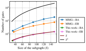
Figure 5: Number of gates versus subgraph size for Erdős–Rényi and Barabási–Albert networks with up to 500 nodes. We consider a fraction $f=0.3$ of nodes to be entangled, and we set $p=0.05$.

In addition to understanding how the gate cost scales with the number of nodes (as presented in Fig. 5), we are interested in understanding how the gate cost depends on graphical properties of the networks. In Fig. 6, we plot the gate cost as a function of the parameter $p$ characterizing the ER and BA network models. In both models, the parameter $p$ gives an indication of the density of the network, with larger values of $p$ indicating higher density. Intuitively, as the density increases, we might expect the gate cost to decrease; however, as we can see in Fig. 6 (left), for the MMG protocol the gate cost actually increases with $p$. In contrast, our protocol maintains a nearly constant number of gates because the size of the subgraph does not change beyond a certain value of $p$, as we can see in Fig. 6 (right). In particular, beyond that value of $p$, the connected subgraph obtained from Protocol 4 contains only those nodes that are to be entangled, with no additional nodes.

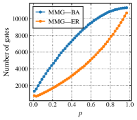
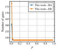
Figure 6: Gate cost versus $p$ for Erdős–Rényi and Barabási–Albert networks with 500 nodes and a fraction $f=0.3$ of nodes to be entangled.

In Fig. 7, we consider the Waxman model, which incorporates the distance between nodes to better reflect realistic networks. We set $\beta$ to unity, and we set the attenuation length between any two nodes to be $L_{0}=22~\text{km}$. Because the Waxman model does not always produce a connected graph, we focus on the largest connected component when analyzing this model. In this model, the largest connected component undergoes a phase transition with respect to diameter; see Fig. 7(a). This phase transition is also reflected in the change of density of the largest connected component, as shown in Fig. 7(b). In Fig. 7(c), for networks with 500 nodes, we can also see the effect of the phase transition on the gate cost of our protocol. Finally, in Fig. 7(d), we show how the gate cost varies with the size of the largest connected component. As with Fig. 5, the results are in agreement with the analytical results of Sec. III.1. We observe multiple values for the gate cost when $S=500$, which reflects the dependence of the gate cost of the MMG protocol [49] on the density of the graph.

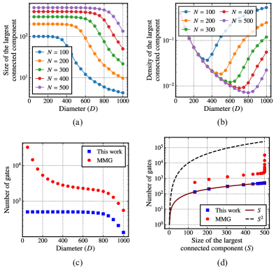
Figure 7: Results for the Waxman model with $\beta=1$ and $L_{0}=22~\text{km}$. (a) and (b): size and density of the largest connected component as a function of diameter. (c): Gate cost as a function of diameter for networks with 500 nodes. (d): Gate cost as a function of the size of the largest connected component.

Let us now consider the number of consumed Bell pairs. In particular, it is of interest to know, particularly in the subset case, how close to optimal is the number of Bell pairs consumed using Protocol 4 compared to using the Steiner tree. In Fig. 8, we plot the ratio of the size of the subgraph to the size of the subset (i.e., the number of nodes to be entangled). This ratio tells us how many additional nodes are needed in the subgraph generated by our Protocol 4 compared to the Steiner tree subgraph (generated using the protocol of Ref. [65]). We can see that for both the BA and ER models, the ratio of our subgraph is close to that of the Steiner tree, implying the number of consumed Bell pairs is also close. In particular, the ratios appear to be getting closer as the total number $N$ of nodes increases, indicating that our protocol may be optimal asymptotically.

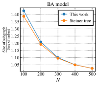
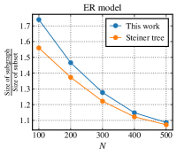
Figure 8: Ratio of the subgraph size to the number of nodes to be entangled, as a function of the total number of nodes, for both the Steiner tree algorithm [65] and our Protocol 4. We consider the Erdős–Rényi and Barabási–Albert models with $p=0.05$ and a fraction $f=0.1$ of nodes to be entangled.

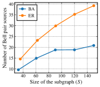
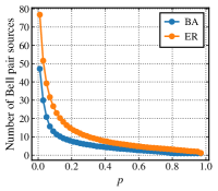
Figure 9: The number of Bell pair sources needed as a function of the subgraph size (left) and the parameter $p$ (right), for both the Erdős–Rényi and Barabási–Albert models. The results are for networks with 500 nodes, $p=0.05$, and a fraction $f=0.3$ of nodes to be entangled.

Finally, we consider the number of Bell pairs sources needed in our protocol; see Fig. 9. The BA model requires fewer Bell pair sources than the ER model. As the parameter $p$ increases, the number of Bell pair sources decreases, as expected.

V Performance with noise

How does our protocol perform in the presence of noise? In this section, we consider the case that both the Bell pairs, the locally-created GHZ states, and the local gates are noisy. We present formulas for the fidelity of the GHZ state after Protocol 2 and Protocol 3.

Theorem 9 (Fidelity after Protocol 2).

If in Protocol 2 the Bell pairs are noisy and given by arbitrary two-qubit density operators $\rho_{A_{1}B_{1}}^{1},\rho_{A_{2}B_{2}}^{2},\dotsc,\rho_{A_{n}B_{n}}^{n}$, then the fidelity of the state after Protocol 2 with respect to the target GHZ state is given by

$$\sum_{\vec{z}\in\{0,1\}^{n-1}}\langle\Phi^{z^{\prime},0}|\rho_{A_{1}B_{1}}^{1}|\Phi^{z^{\prime},0}\rangle\langle\Phi^{z_{1},0}|\rho_{A_{2}B_{2}}^{2}|\Phi^{z_{1},0}\rangle\\ \times\langle\Phi^{z_{2},0}|\rho_{A_{3}B_{3}}^{3}|\Phi^{z_{2},0}\rangle\dotsb\langle\Phi^{z_{n-1},0}|\rho_{A_{n}B_{n}}^{n}|\Phi^{z_{n-1},0}\rangle,$$ (7)

where for every $\vec{z}=(z_{1},z_{2},\dotsc,z_{n-1})\in\{0,1\}^{n-1}$, we have let $z^{\prime}=z_{1}\oplus z_{2}\oplus\dotsb\oplus z_{n-1}$. We have also made use of the Bell state vectors

$$|\Phi^{z,x}\rangle\coloneqq(Z^{z}X^{x}\otimes\mathbbm{1})|\Phi\rangle,$$ (8)

for $z,x\in\{0,1\}$.

Proof.

See App. D.1.  $\blacksquare$

We emphasize that the expression in (7) holds for arbitrary two-qubit density operators. In other words, the expression holds for noisy Bell pairs with an arbitrary noise model. Also, let us observe that the expression for the fidelity in (7) only involves the diagonal elements of the noisy Bell pairs with respect to the Bell basis. Not only that, but only the diagonal elements with respect to the vectors $|\Phi^{0,0}\rangle\equiv|\Phi\rangle=\frac{1}{\sqrt{2}}(|0,0\rangle+|1,1\rangle)$ and $|\Phi^{1,0}\rangle=\frac{1}{\sqrt{2}}(|0,0\rangle-|1,1\rangle)$ are involved. This means, in particular, that if every noisy Bell pair $\rho_{A_{i}B_{i}}^{i}$ is of the form $\rho_{A_{i}B_{i}}^{i}=(1-\mu)|\Phi\rangle\!\langle\Phi|+\mu|\Phi^{1,0}\rangle\!\langle\Phi^{1,0}|$ (i.e., the Bell pairs undergo dephasing noise with parameter $\mu\in[0,1]$), then $\langle\Phi^{z,0}|\rho_{A_{i}B_{i}}^{i}|\Phi^{z,0}\rangle=\mu^{z}(1-\mu)^{1-z}$ for $z\in\{0,1\}$, which means that the fidelity in (7) is equal to

$$\sum_{\vec{z}\in\{0,1\}^{n-1}}\mu^{z^{\prime}}(1-\mu)^{1-z^{\prime}}\mu^{\left|\vec{z}\right|}(1-\mu)^{n-1-\left|\vec{z}\right|}$$

$$\quad=(1-\mu)\sum_{\begin{subarray}{c}\vec{z}\in\{0,1\}^{n-1}\\ \left|\vec{z}\right|\text{ even}\end{subarray}}\mu^{\left|\vec{z}\right|}(1-\mu)^{n-1-\left|\vec{z}\right|}$$

$$\quad\quad+\mu\sum_{\begin{subarray}{c}\vec{z}\in\{0,1\}^{n-1}\\ \left|\vec{z}\right|\text{ odd}\end{subarray}}\mu^{\left|\vec{z}\right|}(1-\mu)^{n-1-\left|\vec{z}\right|}$$ (9)

$$\quad=\frac{1}{2}(1+(1-2\mu)^{n}).$$ (10)

Theorem 10 (Fidelity after Protocol 3).

If in Protocol 3 the GHZ states are noisy and given by arbitrary density operators $\rho_{A_{1}B_{1:n}}^{1}$ and $\rho_{A_{2}C_{1:m}}^{2}$, then the fidelity of the state after Protocol 3 with respect to the target GHZ state is given by

$$\sum_{z\in\{0,1\}}\langle\text{GHZ}_{n+1}^{(z,\vec{0})}|\rho_{A_{1}B_{1:n}}^{1}|\text{GHZ}_{n+1}^{(z,\vec{0})}\rangle\\ \times\langle\text{GHZ}_{m+1}^{(z,\vec{0})}|\rho_{A_{2}C_{1:m}}^{2}|\text{GHZ}_{m+1}^{(z,\vec{0})}\rangle,$$ (11)

where

$$|\text{GHZ}_{n}^{(z,\vec{x})}\rangle\coloneqq(Z^{z}\otimes X^{\vec{x}})|\text{GHZ}_{n}\rangle,$$ (12)

with $z\in\{0,1\}$ and $\vec{x}\in\{0,1\}^{n-1}$, is the $n$-qubit GHZ basis.

Proof.

See App. E.2.1.  $\blacksquare$

Similarly to the fidelity analysis of Protocol 2, we note that for Protocol 3 only the diagonal elements of the noisy GHZ states with respect to the GHZ basis are relevant; in particular, only the fidelities of the noisy GHZ states with respect to $|\text{GHZ}_{n}^{(0,\vec{0})}\rangle\equiv|\text{GHZ}_{n}\rangle=\frac{1}{\sqrt{2}}(|0\rangle^{\otimes n}+|1\rangle^{\otimes n})$ and $|\text{GHZ}_{n}^{(1,\vec{0})}\rangle=\frac{1}{\sqrt{2}}(|0\rangle^{\otimes n}-|1\rangle^{\otimes n})$ are relevant. This means that we can, without loss of generality, consider noisy GHZ states in which one of the qubits undergoes dephasing noise. Therefore, let

$$\rho_{A_{1}B_{1:n}}^{1} =(1-\mu_{1})|\text{GHZ}_{n+1}\rangle\!\langle\text{GHZ}_{n+1}|$$

$$\qquad\qquad+\mu_{1}|\text{GHZ}_{n+1}^{(1,\vec{0})}\rangle\!\langle\text{GHZ}_{n+1}^{(1,\vec{0})}|,$$ (13)

$$\rho_{A_{2}C_{1:m}}^{2} =(1-\mu_{2})|\text{GHZ}_{m+1}\rangle\!\langle\text{GHZ}_{m+1}|$$

$$\qquad\qquad+\mu_{2}|\text{GHZ}_{m+1}^{(1,\vec{0})}\rangle\!\langle\text{GHZ}_{m+1}^{(1,\vec{0})}|,$$ (14)

where $\mu_{1},\mu_{2}\in[0,1]$ are the dephasing parameters. Then, the fidelity in (11) is equal to

$$\sum_{z\in\{0,1\}}\mu_{1}^{z}(1-\mu_{1})^{1-z}\mu_{2}^{z}(1-\mu_{2})^{1-z}\\ =\mu_{1}\mu_{2}+(1-\mu_{1})(1-\mu_{2}).$$ (15)

If $\mu_{1}=\mu_{2}=\mu$, then this simplifies to $1-2\mu+2\mu^{2}$.

In App. E, we provide a more general version of Protocol 3, in which we can merge more than two GHZ states, along with a generalization of Theorem 10.

Now, in addition to noise on the input states of Protocol 2 and Protocol 3, we want to consider noise in the local CNOT gates of these protocols. In App. D.2, we provide an analysis of Protocol 2 in which the CNOT gate is noisy, in addition to the noisy input Bell pairs. In the case of arbitrary Pauli noise acting on the CNOT gates, we can prove that noise can be shifted onto the noisy Bell states, because of the fact that the CNOT gate is a Clifford gate. Consequently, the expression in (7) holds even when the CNOT gate is impacted by arbitrary Pauli noise. If the CNOT gate is impacted by more general noise, then in App. D.2 we provide a general expression for the fidelity after Protocol 2. Analogous reasoning holds for the fidelity after Protocol 3.

VI Summary and outlook

In this work, we consider the distribution of GHZ states in arbitrary Bell-pair networks. While this task is not new, we adopt a novel perspective on evaluating protocols to achieve this task by considering the gate cost of the protocol, in addition to the number of Bell pairs used. We also consider the number of Bell pair sources needed to distribute the GHZ state. Notably, the gate count imposes a more restricted form of local operations and classical communications (LOCC). Unlike the traditional LOCC framework, in which all local operations are considered free, our approach emphasizes the constraints associated with gate usage.

We present protocols for GHZ state entanglement distribution that use a number of gates that is linear in the size of the subgraph corresponding to the desired nodes to be entangled. Notably, this gate cost is independent of the structure and topology of the network. On the other hand, we prove that the MMG protocol [49] requires a number of gates that is at most quadratic in the size of the corresponding subgraph, and we demonstrate numerically that our protocol indeed has reduced gate cost compared to the MMG protocol.

To minimize the number of consumed Bell pairs when distributing a GHZ state among a subset of nodes in a network, a Steiner tree must be identified; however, the Steiner tree problem is NP-hard [62]. It is therefore interesting to ask whether other, polynomial-time strategies can be employed to distribute a GHZ state, while still maintaining near-optimal Bell pair consumption. We affirmatively answer this question by proposing an alternative protocol that identifies connected subgraphs using the breadth-first search (BFS) algorithm. While this approach does not yield the optimal Bell pair count, it avoids the need to find Steiner trees, it runs in polynomial time, and we provide numerical evidence that it achieves near-optimal Bell pair consumption. Furthermore, because our approach does not necessarily require finding a tree, it has better time complexity compared to polynomial-time Steiner tree approximation algorithms [64, 65, 66].

To evaluate our protocols, we performed Monte Carlo simulations on Erdős–Rényi, Barabási–Albert, and Waxman random network models, which represent increasingly realistic network models. For these models, our protocol shows enhanced performance compared to the MMG protocol in dense networks, achieving a nearly quadratic advantage compared to the MMG protocol by minimizing the number of gates required while keeping the number of Bell pairs as low as possible. Furthermore, to our knowledge, the number of Bell pair sources has not been considered in previous works, although it contributes to the resource cost. We therefore also conducted a numerical study to evaluate the number of Bell pair sources required. Additionally, we analyzed our protocol in the context of noisy Bell pairs and noisy gates, and we provided explicit analytic expressions for the fidelity of the states after our protocols for any general noise model.

Future directions.

While our current focus is on creating GHZ states, exploring the merging of other graph states, such as cluster states, could significantly enhance the protocol’s relevance for distributed and measurement-based quantum computing. Additionally, investigating the robustness of this approach against link and node failures is of particular interest, especially in light of classical and quantum research on network resilience, as demonstrated by Refs. [71, 72, 73, 74]. Notably, Ref. [71] demonstrates that small-world networks exhibit robustness to link and node failures. We anticipate that our protocol will be similarly robust, as it is designed to operate effectively within small-world network structures. In the presence of link and node failures, it is also relevant to determine the waiting time of our protocol, and this would generalize studies on the waiting time of linear repeater chains for bipartite entanglement, e.g., Refs. [75, 76], to the multipartite setting.

Currently, our protocol requires full, global knowledge of the network. Therefore, developing protocols that rely primarily on local knowledge and require only a few rounds of classical communication to establish global awareness, leveraging the ideas of, e.g., Ref. [77], would be beneficial.

Identifying stars with the maximum number of leaf nodes is crucial for reducing the number of Bell pair sources, and doing so is an interesting direction for future work. In pursuing this direction, the concept of star covering problem [78] is relevant and would be useful.

Beyond theoretical studies, implementing our algorithm on various experimental platforms is also of great interest. Another intriguing approach is to add an optimization layer to enhance the way the stars are selected and merged, particularly in the context of lossy Bell pairs and lossy memory stations. In principle, this can be accomplished using reinforcement learning, as our problem can be expressed as a Markov decision process (MDP), leveraging the tools from Refs. [79, 80, 81, 82, 83, 76]. Moreover, employing further tools such as (probability) generating functions, the protocols could be optimized in the presence of noise [84, 85].

Appendix A Relation to prior work

Prior work on the distribution of multipartite entanglement in genuine network settings, going beyond repeater chains, includes Refs. [40, 86, 36, 87, 37, 49, 88, 89, 42, 90, 74, 43, 91, 92]. Below, we highlight and compare our work to some of the most relevant of these prior works.

• Reference [40] considers the distribution of arbitrary graph states, in which the graph of the corresponding graph state matches the topology of the underlying network of Bell pairs.

• Reference [42] involves local preparation of the desired graph state, followed by teleportation of the state to the desired parties using the Bell pair network, which can be arbitrary. The basis of their protocol is the so-called “Bipartite A” protocol of Ref. [40]. Essentially, their protocol is the Bipartite A protocol supplemented by an analysis of completion time based on particular algorithms for finding paths in the Bell-pair network for the purpose of teleporting the locally-created graph state.

• Reference [43] considers the distribution of GHZ states in a star Bell-pair network topology, in which the central “factory” node locally produces the GHZ states and then uses the Bell pairs to teleport it to the outer parties. This is also essentially the Bipartite A protocol of Ref. [40], with noisy Bell pairs and an analysis of the rate at which the GHZ states can be distributed.

• Reference [49] uses the Steiner tree, along with a sub-routine called “star expansion”, to distribution a GHZ state between a given set of nodes in the network.

• Reference [90] also makes use of the Steiner tree problem, and includes an analysis with noisy Bell pairs.

• Similarly to Ref. [43], Ref. [93] requires a star Bell-pair topology. Here, an arbitrary graph state can be produced using a “subgraph complementation system” associated with the graph of the desired graph state. Reference [92] also considers a star topology only.

Appendix B Overview of graph states

A graph state [94, 12, 95] is a multi-qubit quantum state defined using graphs. Consider a graph $G=(V,E)$, which consists of a set $V$ of vertices and a set $E$ of edges. For the purposes of this example, $G$ is an undirected graph, and $E$ is a set of two-element subsets of $V$. The graph state $|G\rangle$ is an $n$-qubit quantum state $|G\rangle_{A_{1}\dotsb A_{n}}$, with $n=|V|$, that is defined as

$$|G\rangle_{A_{1}\dotsb A_{n}}\coloneqq\frac{1}{\sqrt{2^{n}}}\sum_{\vec{x}\in\{0,1\}^{n}}(-1)^{\frac{1}{2}\vec{x}^{{\scriptscriptstyle\mathsf{T}}}M_{G}\vec{x}}|\vec{\alpha}\rangle,$$ (16)

where $M_{G}$ is the adjacency matrix of $G$, which is defined as

$$(M_{G})_{i,j}=\left\{\begin{array}[]{l l}1&\text{if }\{v_{i},v_{j}\}\in E,\\ 0&\text{otherwise},\end{array}\right.$$ (17)

and $\vec{x}$ is the column vector $(x_{1},x_{2},\dotsc,x_{n})^{{\scriptscriptstyle\mathsf{T}}}$. It is straightforward to show that

$$|G\rangle_{A_{1}\dotsb A_{n}}=\text{CZ}(G)(|+\rangle_{A_{1}}\otimes\dotsb\otimes|+\rangle_{A_{n}}),$$ (18)

where $|+\rangle\coloneqq\frac{1}{\sqrt{2}}(|0\rangle+|1\rangle)$ and

$$\text{CZ}(G)\coloneqq\bigotimes_{\{v_{i},v_{j}\}\in E}\text{CZ}_{A_{i}A_{j}},$$ (19)

with $\text{CZ}_{A_{i}A_{j}}\coloneqq|0\rangle\!\langle 0|_{A_{i}}\otimes\mathbbm{1}_{A_{j}}+|1\rangle\!\langle 1|_{A_{i}}\otimes Z_{A_{j}}$ being the controlled-$Z$ gate.

Consider a star graph of $n$ nodes, labeled $\{1,2,\dotsc,n\}$, such that the center of the star is node $k\in\{1,2,\dotsc,n\}$. We denote this graph by $S_{n,k}$. It is straightforward to show that the graph state corresponding to this graph, defined equivalently according to (16) or (18), is

$$|S_{n,k}\rangle=(H^{\otimes(k-1)}\otimes\mathbbm{1}\otimes H^{\otimes n-k})|\text{GHZ}_{n}\rangle,$$ (20)

where $H=|+\rangle\!\langle 0|+|-\rangle\!\langle 1|=\frac{1}{\sqrt{2}}\begin{pmatrix}1&1\\ 1&-1\end{pmatrix}$ is the Hadamard operator and $|-\rangle=\frac{1}{\sqrt{2}}(|0\rangle-|1\rangle)$. This means that the star graph state is equivalent to the GHZ state up to local Hadamard gates. In particular, observe in (20) that the center of the star graph (namely, the $k$-th qubit) is the only qubit that does not have a Hadamard gate applied to it. This implies that to change the center of the star graph state involves only two Hadamard gates: one Hadamard gate applied to the current central qubit, and the other Hadamard gate applied to the new central qubit. Note that we apply only two gates to change the center regardless of the size $n$ of the star. We also note that for $n=2$, we have that the two-party GHZ state is equal to the Bell state, i.e., $|\text{GHZ}_{2}\rangle=\frac{1}{\sqrt{2}}(|0,0\rangle+|1,1\rangle)=|\Phi\rangle$. It follows that $|S_{2,1}\rangle=(\mathbbm{1}\otimes H)|\Phi\rangle=(H\otimes\mathbbm{1})|\Phi\rangle=|S_{2,2}\rangle$. Finally, performing an $X$-basis measurement on any subset of the qubits in a GHZ state produces a GHZ state among the remaining qubits, up to a Pauli-$Z$ correction. More precisely, if we measure the first $m<n$ of the qubits of the state $|\text{GHZ}_{n}\rangle$ in the $X$-basis, then we obtain

$$\left(\langle z_{1}|H\otimes\langle z_{2}|H\otimes\dotsb\otimes\langle z_{m}|H\otimes\mathbbm{1}\right)|\text{GHZ}_{n}\rangle=\frac{1}{\sqrt{2^{m}}}(Z^{z_{1}\oplus z_{2}\oplus\dotsb\oplus z_{m}}\otimes\mathbbm{1})|\text{GHZ}_{n-m}\rangle,$$ (21)

for all $z_{1},z_{2},\dotsc,z_{m}\in\{0,1\}$.

Appendix C Graph state distribution in the star topology

Consider the scenario in which $n$ nodes share Bell states with a central node. The task is for the central node to distribute the graph state $|G\rangle$ to the $n$ outer nodes. One possible procedure is for the central node to locally prepare the graph state and then to teleport the individual qubits using the Bell states—this is the “Bipartite A” protocol of Ref. [40]. However, it is possible to perform a slightly simpler procedure that does not require the additional qubits needed to prepare the graph state locally. In fact, the following deterministic procedure produces the required graph state $|G\rangle$ shared by the nodes $A_{1},\dotsc,A_{n}$. It is known as the “Bipartite B” protocol in Ref. [40, Sec. III.B] and is presented in Protocol 5.

Protocol 5 Graph state from Bell pairs in a star topology (Bipartite B protocol of Ref. [40])

1:$n\in\{1,2,\dotsc\}$ Bell pairs $|\Phi\rangle$, $N=n+1$ nodes in a star topology (The central node shares a Bell pair with each of the $n$ outer nodes.); graph $G$ with $N-1=n$ nodes.

2:Graph state $|G\rangle$ shared by the $n$ outer nodes.

3:The central node applies $\text{CZ}(G)$ to its qubits.

4:Measure each central qubit in the Pauli-$X$ basis. The outcome is an $n$-bit string $\vec{x}=(x_{1},\dotsc,x_{n})$. The central node communicates outcome $x_{i}$ to the $i$-th outer node.

5:At the $i$-th outer node: if $x_{i}=0$, then no gate is applied, and if $x_{i}=1$, then the Pauli-$Z$ gate is applied.

We note that Protocol 5 uses $|E|$ two-qubit gates, where $|E|$ is the number of edges in the graph $G$. (We exclude the single-qubit Pauli-gate corrections in the gate count.) It has also been recently shown in Ref. [96] that the Bipartite B protocol is optimal in terms of the communication cost of distributing a graph state in a star Bell-pair topology.

Remark 1.

Note that at the end of this protocol, the central node is not included in the final graph state. We can modify this protocol slightly by adding an additional Bell pair that is contained entirely within the central node, and then doing the protocol just as above. With this modification, the final graph state includes the central node. $\blacktriangleleft$

In Ref. [80, Sec. III.B.3], it is shown explicitly that this protocol achieves the desired graph state $|G\rangle$ between the outer nodes. It is also shown in Ref. [80] that if, instead of perfect Bell pairs, the central node is connected to the outer nodes via imperfect Bell pairs (and if the gates are perfect), then the fidelity of the state at the end of the protocol has fidelity with respect to the desired graph state according to the following formula.

Proposition 11 (Fidelity after the noisy Bipartite B protocol [80]).

Consider a network with a star topology, consisting of $n$ outer nodes. Suppose that the central node shares imperfect Bell pairs with each of the outer nodes, and that these imperfect Bell pairs are represented by arbitrary two-qubit density operators $\rho_{1},\rho_{2},\dotsc,\rho_{n}$. Let $\rho_{\text{final}}$ the state resulting from applying the Bipartite B protocol. The fidelity of $\rho_{\text{final}}$ with respect to a given, desired graph state $|G\rangle$ is equal to the following expression:

$$\langle G|\rho_{\text{final}}|G\rangle=\sum_{\vec{x}\in\{0,1\}^{n}}\langle\Phi^{z_{1},x_{1}}|\rho_{1}|\Phi^{z_{1},x_{1}}\rangle\langle\Phi^{z_{2},x_{2}}|\rho_{2}|\Phi^{z_{2},x_{2}}\rangle\dotsb\langle\Phi^{z_{n},x_{n}}|\rho_{n}|\Phi^{z_{n},x_{n}}\rangle,$$ (22)

where the column vector $\vec{z}=(z_{1},\dotsc,z_{n})^{{\scriptscriptstyle\mathsf{T}}}$ is given by $\vec{z}=A(G)\vec{x}$, with $A(G)$ being the adjacency matrix of the graph $G$. Also, we have used the definition

$$|\Phi^{z,x}\rangle\coloneqq(Z^{z}X^{x}\otimes\mathbbm{1})|\Phi\rangle,\quad|\Phi\rangle\coloneqq\frac{1}{\sqrt{2}}(|0,0\rangle+|1,1\rangle).$$ (23)

Appendix D Analysis of Protocol 2

As mentioned in Remark 1, Protocol 5 creates a final graph state that excludes the central node. In particular, when creating a star graph state using Protocol 5, the central node is not part of the final state. (Recall from (20) that the star graph state is local-unitary equivalent to the GHZ state.) Here, we analyze Protocol 2, which, without any additional Bell pairs, creates a GHZ state that includes the central node.

We start with $n\in\{2,3,\dotsc\}$ Bell pairs $|\Phi\rangle_{A_{1}B_{1}},|\Phi\rangle_{A_{2}B_{2}},\dotsc,|\Phi\rangle_{A_{n}B_{n}}$, where $n\in\{2,3,\dotsc\}$. The following protocol deterministically transforms these Bell pairs into the GHZ state $|\text{GHZ}_{n+1}\rangle_{A_{1}B_{1}\dotsb B_{n}}$. Let us prove that Protocol 2 performs as claimed. We use the abbreviation $A_{1:n}\equiv A_{1}A_{2}\dotsb A_{n}$, similarly for $B_{1:n}$. The initial state is

$$|\Phi\rangle_{A_{1}B_{1}}\otimes|\Phi\rangle_{A_{2}B_{2}}\otimes\dotsb\otimes|\Phi\rangle_{A_{n}B_{n}} =\frac{1}{\sqrt{2^{n}}}\sum_{\vec{\alpha}\in\{0,1\}^{n}}|\vec{\alpha}\rangle_{A_{1:n}}|\vec{\alpha}\rangle_{B_{1:n}}$$ (24)

$$=\frac{1}{\sqrt{2^{n}}}\sum_{\vec{\beta}\in\{0,1\}^{n-1}}\left(|0\rangle_{A_{1}}|\vec{\beta}\rangle_{A_{2:n}}|0\rangle_{B_{1}}|\vec{\beta}\rangle_{B_{2:n}}+|1\rangle_{A_{1}}|\vec{\beta}\rangle_{A_{2:n}}|1\rangle_{B_{1}}|\vec{\beta}\rangle_{B_{2:n}}\right).$$ (25)

Then, after applying the CNOT gates, we obtain

$$\frac{1}{\sqrt{2^{n}}}\sum_{\vec{\beta}\in\{0,1\}^{n-1}}\left(|0\rangle_{A_{1}}|\vec{\beta}\rangle_{A_{2:n}}|0\rangle_{B_{1}}|\vec{\beta}\rangle_{B_{2:n}}+|1\rangle_{A_{1}}|\vec{\beta}\oplus\vec{1}\rangle_{A_{2:n}}|1\rangle_{B_{1}}|\vec{\beta}\rangle_{B_{2:n}}\right)\\ =\frac{1}{\sqrt{2^{n}}}\sum_{\vec{\beta}\in\{0,1\}^{n-1}}\left(|0\rangle_{A_{1}}|\vec{\beta}\rangle_{A_{2:n}}|0\rangle_{B_{1}}|\vec{\beta}\rangle_{B_{2:n}}+|1\rangle_{A_{1}}|\vec{\beta}\rangle_{A_{2:n}}|1\rangle_{B_{1}}|\vec{\beta}\oplus\vec{1}\rangle_{B_{2:n}}\right).$$ (26)

From this, we can see that upon measurement of the qubits $A_{2},A_{3},\dotsc,A_{n}$, we obtain every outcome string $\vec{\beta}\in\{0,1\}^{n-1}$ with probability $\frac{1}{2^{n-1}}$, and conditioned on this outcome the state of the remaining qubits is

$$\frac{1}{\sqrt{2}}\left(|0\rangle_{A_{1}}|0\rangle_{B_{1}}|\vec{\beta}\rangle_{B_{2:n}}+|1\rangle_{A_{1}}|1\rangle_{B_{1}}|\vec{\beta}\oplus\vec{1}\rangle_{B_{2:n}}\right)=X_{B_{2}}^{\beta_{1}}\otimes X_{B_{3}}^{\beta_{2}}\otimes\dotsb\otimes X_{B_{n}}^{\beta_{n-1}}|\text{GHZ}_{n+1}\rangle_{A_{1}B_{1:n}},$$ (27)

where $\beta_{i}\in\{0,1\}$ corresponds to the measurement outcome for the qubit $A_{i}$, $i\in\{2,3,\dotsc,n\}$. With the convention that $X^{0}\equiv\mathbbm{1}$, we see that by applying the Pauli-$X$ gate to every qubit $B_{i}$ whose corresponding measured qubit $A_{i}$ had outcome 1, we obtain the desired GHZ state on the qubits $A_{1},B_{1},B_{2},\dotsc,B_{n}$.

This protocol has the following representation as an LOCC quantum channel:

$$\mathcal{L}(\rho_{A_{1:n}B_{1:n}})=\sum_{\vec{\beta}\in\{0,1\}^{n-1}}\left(\langle\vec{\beta}|_{A_{2:n}}\text{CNOT}_{n}^{\dagger}\otimes X_{B_{2:n}}^{\vec{\beta}}\right)\left(\rho_{A_{1:n}B_{1:n}}\right)\left(\text{CNOT}_{n}|\vec{\beta}\rangle_{A_{2:n}}\otimes X_{B_{2:n}}^{\vec{\beta}}\right),$$ (28)

where we have made use of the abbreviations

$$\text{CNOT}_{n} \equiv\text{CNOT}_{A_{1}A_{n}}\text{CNOT}_{A_{1}A_{n-1}}\dotsb\text{CNOT}_{A_{1}A_{3}}\text{CNOT}_{A_{1}A_{2}},$$ (29)

$$|\vec{\beta}\rangle_{A_{2:n}} \equiv|\beta_{1}\rangle_{A_{2}}\otimes|\beta_{2}\rangle_{A_{3}}\otimes\dotsb\otimes|\beta_{n-1}\rangle_{A_{n}},$$ (30)

$$X_{B_{2:n}}^{\vec{\beta}} \equiv X_{B_{2}}^{\beta_{1}}\otimes X_{B_{3}}^{\beta_{2}}\otimes\dotsb\otimes X_{B_{n}}^{\beta_{n-1}}.$$ (31)

for all $\vec{\beta}=(\beta_{1},\beta_{2},\dotsc,\beta_{n-1})\in\{0,1\}^{n-1}$.

Remark 2.

Protocol 2 can be modified in the case that the inputs are not the Bell state vectors $|\Phi\rangle$ but instead the state vectors $|S_{2,1}\rangle=(\mathbbm{1}\otimes H)|\Phi\rangle$. In this case, the steps of the protocol are exactly as before, except that the correction operations change: instead of applying the Pauli-$X$ to the qubits $B_{2},B_{3},\dotsc,B_{n}$ according to the measurement outcomes, we apply the Pauli-$Z$ gate to those qubits. The result of the protocol is then the star graph state $|S_{n+1,1}\rangle_{A_{1}B_{1:n}}$, with the center at qubit $A_{1}$. $\blacktriangleleft$

D.1 Proof of Theorem 9

Theorem 12 (Restatement of Theorem 9).

Consider a network with a star topology, consisting of $n$ outer nodes. Suppose that the central node shares imperfect Bell pairs with each of the outer nodes, and that these imperfect Bell pairs are represented by arbitrary two-qubit density operators $\rho^{1},\rho^{2},\dotsc,\rho^{n}$.

$$\langle\text{GHZ}_{n+1}|_{A_{1}B_{1:n}}\mathcal{L}\left(\rho_{A_{1}B_{1}}^{1}\otimes\rho_{A_{2}B_{2}}^{2}\otimes\dotsb\otimes\rho_{A_{n}B_{n}}^{n}\right)|\text{GHZ}_{n+1}\rangle_{A_{1}B_{1:n}}\\ =\sum_{\vec{z}\in\{0,1\}^{n-1}}\langle\Phi^{z^{\prime},0}|\rho_{A_{1}B_{1}}^{1}|\Phi^{z^{\prime},0}\rangle\langle\Phi^{z_{1},0}|\rho_{A_{2}B_{2}}^{2}|\Phi^{z_{1},0}\rangle\langle\Phi^{z_{2},0}|\rho_{A_{2}B_{2}}^{2}|\Phi^{z_{2},0}\rangle\dotsb\langle\Phi^{z_{n-1},0}|\rho_{A_{n}B_{n}}^{n}|\Phi^{z_{n-1},0}\rangle,$$ (32)

where $z^{\prime}=z_{1}\oplus z_{2}\oplus\dotsb\oplus z_{n-1}$, and we recall the definition of the Bell states $|\Phi^{z_{i},0}\rangle$ in (23).

Proof.

We start by noting that

$$|v(\vec{\beta})\rangle \coloneqq\left(\text{CNOT}_{n}|\vec{\beta}\rangle_{A_{2:n}}\otimes X_{B_{2:n}}^{\vec{\beta}}\right)|\text{GHZ}_{n+1}\rangle_{A_{1}B_{1:n}}$$ (33)

$$=\frac{1}{\sqrt{2}}\left(\text{CNOT}_{n}|0\rangle_{A_{1}}|\vec{\beta}\rangle_{A_{2:n}}\otimes|0\rangle_{B_{1}}|\vec{\beta}\rangle_{B_{2:n}}+\text{CNOT}_{n}|1\rangle_{A_{1}}|\vec{\beta}\rangle_{B_{2:n}}\otimes|1\rangle_{B_{1}}|\vec{\beta}\oplus\vec{1}\rangle_{B_{2:n}}\right)$$ (34)

$$=\frac{1}{\sqrt{2}}\left(|0\rangle_{A_{1}}|\vec{\beta}\rangle_{A_{2:n}}\otimes|0\rangle_{B_{1}}|\vec{\beta}\rangle_{B_{2:n}}+|1\rangle_{A_{1}}|\vec{\beta}\oplus\vec{1}\rangle_{A_{2:n}}\otimes|1\rangle_{B_{1}}|\vec{\beta}\oplus\vec{1}\rangle_{B_{2:n}}\right)$$ (35)

$$=\frac{1}{\sqrt{2}}\sum_{x\in\{0,1\}}|x\rangle_{A_{1}}|x\rangle_{B_{1}}\bigotimes_{i=1}^{n-1}|\beta_{i}\oplus x\rangle_{A_{i+1}}|\beta_{i}\oplus x\rangle_{B_{i+1}}.$$ (36)

Now, we use the fact that

$$|x\rangle_{A}|x\rangle_{B}=\frac{1}{\sqrt{2}}\sum_{z\in\{0,1\}}(-1)^{xz}|\Phi^{z,0}\rangle,$$ (37)

for all $x\in\{0,1\}$. With this, we obtain

$$|v(\vec{\beta})\rangle =\frac{1}{\sqrt{2}}\frac{1}{\sqrt{2^{n}}}\sum_{x\in\{0,1\}}\sum_{z_{0},z_{1},\dotsc,z_{n-1}\in\{0,1\}}(-1)^{xz_{0}}|\Phi^{z_{0},0}\rangle_{A_{1}B_{1}}\bigotimes_{i=1}^{n-1}\sum_{z_{i}\in\{0,1\}}(-1)^{(\beta_{i}\oplus x)z_{i}}|\Phi^{z_{i},0}\rangle_{A_{i+1}B_{i+1}}$$ (38)

$$=\frac{1}{\sqrt{2}}\frac{1}{\sqrt{2^{n}}}\sum_{z_{0},z_{1},\dotsc,z_{n-1}\in\{0,1\}}\sum_{x\in\{0,1\}}(-1)^{x(z_{0}+z_{1}+\dotsb+z_{n-1})}(-1)^{\beta_{1}z_{1}+\beta_{2}z_{2}+\dotsb+\beta_{n-1}z_{n-1}}|\Phi^{z_{0},0}\rangle_{A_{1}B_{1}}\bigotimes_{i=1}^{n-1}|\Phi^{z_{i},0}\rangle_{A_{i+1}B_{i+1}}$$ (39)

$$=\frac{1}{\sqrt{2^{n-1}}}\sum_{\vec{z}\in\{0,1\}^{n-1}}(-1)^{\vec{\beta}\cdot\vec{z}}|\Phi^{z^{\prime},0}\rangle_{A_{1}B_{1}}\bigotimes_{i=1}^{n-1}|\Phi^{z_{i},0}\rangle_{A_{i+1}B_{i+1}},$$ (40)

where for the final equality we used the fact that

$$\sum_{x\in\{0,1\}}(-1)^{x(z_{0}+z_{1}+\dotsb+z_{n-1})}=2\delta_{z_{0}+z_{1}+\dotsb+z_{n-1},0}=2\delta_{z_{0},z_{1}\oplus z_{2}\oplus\dotsb\oplus z_{n-1}},$$ (41)

and we let $z^{\prime}\equiv z_{1}\oplus z_{2}\oplus\dotsb\oplus z_{n-1}$. Therefore, for any arbitrary state $\rho_{A_{1:n}B_{1:n}}$, we have

$$\langle\text{GHZ}_{n+1}|_{A_{1}B_{1:n}}\mathcal{L}\left(\rho_{A_{1:n}B_{1:n}}\right)|\text{GHZ}_{n+1}\rangle_{A_{1}B_{1:n}}$$

$$\quad=\sum_{\vec{\beta}\in\{0,1\}^{n-1}}\langle v(\vec{\beta})|\rho_{A_{1:n}B_{1:n}}|v(\beta)\rangle$$ (42)

$$\quad=\frac{1}{2^{n-1}}\sum_{\vec{\beta},\vec{z},\vec{y}\in\{0,1\}^{n-1}}(-1)^{\vec{\beta}\cdot\vec{z}}(-1)^{\vec{\beta}\cdot\vec{y}}\left(\langle\Phi^{z^{\prime},0}|_{A_{1}B_{1}}\bigotimes_{i=1}^{n-1}\langle\Phi^{z_{i},0}|_{A_{i+1}B_{i+1}}\right)\left(\rho_{A_{1:n}B_{1:n}}\right)\left(|\Phi^{y^{\prime},0}\rangle_{A_{1}B_{1}}\bigotimes_{i=1}^{n-1}|\Phi^{y_{i},0}\rangle_{A_{i+1}B_{i+1}}\right)$$ (43)

$$\quad=\sum_{\vec{z}\in\{0,1\}^{n-1}}\left(\langle\Phi^{z^{\prime},0}|_{A_{1}B_{1}}\bigotimes_{i=1}^{n-1}\langle\Phi^{z_{i},0}|_{A_{i+1}B_{i+1}}\right)\left(\rho_{A_{1:n}B_{1:n}}\right)\left(|\Phi^{z^{\prime},0}\rangle_{A_{1}B_{1}}\bigotimes_{i=1}^{n-1}|\Phi^{z_{i},0}\rangle_{A_{i+1}B_{i+1}}\right),$$ (44)

where to obtain the final equality we used the fact that

$$\sum_{\vec{\beta}\in\{0,1\}^{n-1}}(-1)^{\vec{\beta}\cdot\vec{z}}(-1)^{\vec{\beta}\cdot\vec{y}}=\sum_{\vec{\beta}\in\{0,1\}^{n-1}}(-1)^{\vec{\beta}\cdot(\vec{z}\oplus\vec{y})}=2^{n-1}\delta_{\vec{z},\vec{y}},$$ (45)

for all $\vec{z},\vec{y}\in\{0,1\}^{n-1}$. As (44) holds for all states $\rho_{A_{1:n}B_{1:n}}$, it holds also for the tensor-product state in the statement of the proposition. The proof is therefore complete.  $\blacksquare$

D.2 Adding noise to the CNOT gates

In Proposition 11, we considered noise only in the initial Bell states. Let us now consider noise in the CNOT gates as well. First, let us recall that the two-qubit CNOT gate has the form $\text{CNOT}=|0\rangle\!\langle 0|\otimes\mathbbm{1}+|1\rangle\!\langle 1|\otimes X$, where $X$ is the Pauli-$X$ gate. Then, it is straightforward to show that

$$\text{CNOT}_{n}=|0\rangle\!\langle 0|\otimes\mathbbm{1}^{\otimes(n-1)}+|1\rangle\!\langle 1|\otimes X^{\otimes(n-1)}.$$ (46)

Now, for illustrative purposes, as our model of the noisy $\text{CNOT}_{n}$ gate, let us assume IID noise on all of the qubits after the ideal $\text{CNOT}_{n}$ gate, represented by the single-qubit quantum channel $\mathcal{N}$. The noisy version of the $\text{CNOT}_{n}$ gate is then simply the quantum channel $(\cdot)\mapsto\mathcal{N}^{\otimes n}(\text{CNOT}_{n}(\cdot)\text{CNOT}_{n})$.

Now, if the noise channel $\mathcal{N}$ is a Pauli channel, then it can be written as $\mathcal{N}(\cdot)=p_{I}(\cdot)+p_{X}X(\cdot)X+p_{Y}Y(\cdot)Y+p_{Z}Z(\cdot)Z$, where the quantities $p_{I},p_{X},p_{Y},p_{Z}$ form a probability distribution, such that $\mathcal{N}^{\otimes n}=\sum_{P\in\{\mathbbm{1},X,Y,Z\}^{\otimes n}}p_{P}P(\cdot)P$. Then, the noisy $\text{CNOT}_{n}$ gate is

$$\sum_{P\in\{\mathbbm{1},X,Y,Z\}^{\otimes n}}p_{P}P\text{CNOT}_{n}(\cdot)\text{CNOT}_{n}P.$$ (47)

Now, because $\text{CNOT}_{n}$ is a Clifford gate, it holds that $P\text{CNOT}_{n}=\text{CNOT}_{n}P^{\prime}$, where $P^{\prime}\in\{\mathbbm{1},X,Y,Z\}^{\otimes n}$ is some other $n$-qubit Pauli operator. (This is true because, essentially by definition, Clifford gates map Pauli operators to other Pauli operators.) Therefore, our noisy $\text{CNOT}_{n}$ gate is equivalently given by

$$\sum_{P\in\{\mathbbm{1},X,Y,Z\}^{\otimes n}}p_{P}\text{CNOT}_{n}P^{\prime}(\cdot)P^{\prime}\text{CNOT}_{n}=\text{CNOT}_{n}\mathcal{N}^{\prime}(\cdot)\text{CNOT}_{n},$$ (48)

where $\mathcal{N}^{\prime}(\cdot)\equiv\sum_{P\in\{\mathbbm{1},X,Y,Z\}^{\otimes n}}p_{P}P^{\prime}(\cdot)P^{\prime}$ is another Pauli channel. In other words, when the noise is any Pauli channel, the $\text{CNOT}_{n}$ gate can be brought outside of the action of the noise, and can therefore be absorbed into the state $\rho_{A_{1:n}B_{1:n}}$ in Proposition 11. This means that Proposition 11—specifically, the expression in (44)—holds even when the $\text{CNOT}_{n}$ gate is impacted by arbitrary Pauli noise.

If the noise channel $\mathcal{N}$ is not a Pauli channel, but instead an arbitrary quantum channel, then the expression in (44) generalizes to the expression in (69) below, which we now prove. To start with, we generally have that $\mathcal{N}^{\otimes n}(\cdot)=\sum_{j=1}^{r}K^{(j)}(\cdot)K^{(j)\dagger}$, where $\{K^{(j)}\}_{j=1}^{r}$ are the Kraus operators. Therefore, the noisy version of the channel in (28) is given by

$$\widetilde{\mathcal{L}}(\rho_{A_{1:n}B_{1:n}}) =\sum_{\vec{\beta}\in\{0,1\}^{n-1}}\left(\langle\vec{\beta}|_{A_{2:n}}\otimes X_{B_{2:n}}^{\vec{\beta}}\right)\mathcal{N}_{A_{1:n}}^{\otimes n}\left(\text{CNOT}_{A_{1:n}}(\rho_{A_{1:n}B_{1:n}})\text{CNOT}_{A_{1:n}}\right)\left(|\vec{\beta}\rangle_{A_{2:n}}\otimes X_{B_{2:n}}^{\vec{\beta}}\right)$$ (49)

$$=\sum_{\vec{\beta}\in\{0,1\}^{n-1}}\sum_{j=1}^{r}\left(\langle\vec{\beta}|_{A_{2:n}}K_{A_{1:n}}^{(j)}\text{CNOT}_{A_{1:n}}\otimes X_{B_{2:n}}^{\vec{\beta}}\right)\left(\rho_{A_{1:n}B_{1:n}}\right)\left(\text{CNOT}_{A_{1:n}}K_{A_{1:n}}^{(j)\dagger}|\vec{\beta}\rangle_{A_{2:n}}\otimes X_{B_{2:n}}^{\vec{\beta}}\right),$$ (50)

where $\rho_{A_{1:n}B_{1:n}}$ is an arbitrary quantum state. Similarly to before, can now define the vector

$$|v(\vec{\beta},j)\rangle \coloneqq\left(\text{CNOT}_{A_{1:n}}K_{A_{1:n}}^{(j)\dagger}|\vec{\beta}\rangle_{A_{2:n}}\otimes X_{B_{2:n}}^{\vec{\beta}}\right)|\text{GHZ}_{n+1}\rangle_{A_{1}B_{1:n}}$$ (51)

$$=\frac{1}{\sqrt{2}}\left(\text{CNOT}_{A_{1:n}}K_{A_{1:n}}^{(j)\dagger}|0\rangle_{A_{1}}|\vec{\beta}\rangle_{A_{2:n}}\otimes|0\rangle_{B_{1}}|\vec{\beta}\rangle_{B_{2:n}}+\text{CNOT}_{A_{1:n}}K_{A_{1:n}}^{(j)\dagger}|1\rangle_{A_{1}}|\vec{\beta}\rangle_{A_{2:n}}\otimes|1\rangle_{B_{1}}|\vec{\beta}\oplus\vec{1}\rangle_{B_{2:n}}\right),$$ (52)

such that

$$\langle\text{GHZ}_{n+1}|_{A_{1}B_{1:n}}\widetilde{\mathcal{L}}(\rho_{A_{1:n}B_{1:n}})|\text{GHZ}_{n+1}\rangle_{A_{1}B_{1:n}}=\sum_{\vec{\beta}\in\{0,1\}^{n-1}}\sum_{j=1}^{r}\langle v(\vec{\beta},j)|\rho_{A_{1:n}B_{1:n}}|v(\vec{\beta},j)\rangle.$$ (53)

Now,

$$\text{CNOT}_{A_{1:n}}K_{A_{1:n}}^{(j)\dagger}|0\rangle_{A_{1}}|\vec{\beta}\rangle_{A_{2:n}} =\left(|0\rangle\!\langle 0|_{A_{1}}\otimes\mathbbm{1}_{A_{2:n}}^{\otimes(n-1)}+|1\rangle\!\langle 1|_{A_{1}}\otimes X_{A_{2:n}}^{\otimes(n-1)}\right)K_{A_{1:n}}^{(j)\dagger}|0\rangle_{A_{1}}|\vec{\beta}\rangle_{A_{2:n}}$$ (54)

$$=|0\rangle_{A_{1}}\langle 0|_{A_{1}}K_{A_{1:n}}^{(j)\dagger}|0\rangle_{A_{1}}|\vec{\beta}\rangle_{A_{2:n}}+|1\rangle_{A_{1}}X_{A_{2:n}}^{\otimes(n-1)}\langle 1|_{A_{1}}K_{A_{1:n}}^{(j)\dagger}|0\rangle_{A_{1}}|\vec{\beta}\rangle_{A_{2:n}}$$ (55)

$$\equiv|0\rangle_{A_{1}}K_{A_{2:n}}^{(j,0,0)}|\vec{\beta}\rangle_{A_{2:n}}+|1\rangle_{A_{1}}X_{A_{2:n}}^{\otimes(n-1)}K_{A_{2:n}}^{(j,1,0)}|\vec{\beta}\rangle_{A_{2:n}},$$ (56)

$$\text{CNOT}_{A_{1:n}}K_{A_{1:n}}^{(j)\dagger}|1\rangle_{A_{1}}|\vec{\beta}\rangle_{A_{2:n}} =\left(|0\rangle\!\langle 0|_{A_{1}}\otimes\mathbbm{1}_{A_{2:n}}^{\otimes(n-1)}+|1\rangle\!\langle 1|_{A_{1}}\otimes X_{A_{2:n}}^{\otimes(n-1)}\right)K_{A_{1:n}}^{(j)\dagger}|1\rangle_{A_{1}}|\vec{\beta}\rangle_{A_{2:n}}$$ (57)

$$=|0\rangle_{A_{1}}\langle 0|_{A_{1}}K_{A_{1:n}}^{(j)\dagger}|1\rangle_{A_{1}}|\vec{\beta}\rangle_{A_{2:n}}+|1\rangle_{A_{1}}X_{A_{2:n}}^{\otimes(n-1)}\langle 1|_{A_{1}}K_{A_{1:n}}^{(j)\dagger}|1\rangle_{A_{1}}|\vec{\beta}\rangle_{A_{2:n}}$$ (58)

$$\equiv|0\rangle_{A_{1}}K_{A_{2:n}}^{(j,0,1)}|\vec{\beta}\rangle_{A_{2:n}}+|1\rangle_{A_{1}}X_{A_{2:n}}^{\otimes(n-1)}K_{A_{2:n}}^{(j,1,1)}|\vec{\beta}\rangle_{A_{2:n}},$$ (59)

where we have let $K_{A_{2:n}}^{(j,a,b)}\equiv\langle a|_{A_{1}}K_{A_{1:n}}^{(j)\dagger}|b\rangle_{A_{1}}$, for $a,b\in\{0,1\}$. Therefore,

$$|v(\vec{\beta},j)\rangle =\frac{1}{\sqrt{2}}\left(|0\rangle_{A_{1}}K_{A_{2:n}}^{(j,0,0)}|\vec{\beta}\rangle_{A_{2:n}}\otimes|0\rangle_{B_{1}}|\vec{\beta}\rangle_{B_{2:n}}+|1\rangle_{A_{1}}X_{A_{2:n}}^{\otimes(n-1)}K_{A_{2:n}}^{(j,1,0)}|\vec{\beta}\rangle_{A_{2:n}}\otimes|0\rangle_{B_{1}}|\vec{\beta}\rangle_{B_{2:n}}\right.$$

$$\qquad\qquad\left.+|0\rangle_{A_{1}}K_{A_{2:n}}^{(j,0,1)}|\vec{\beta}\rangle_{A_{2:n}}\otimes|1\rangle_{B_{1}}|\vec{\beta}\oplus\vec{1}\rangle_{B_{2:n}}+|1\rangle_{A_{1}}X_{A_{2:n}}^{\otimes(n-1)}K_{A_{2:n}}^{(j,1,1)}|\vec{\beta}\rangle_{A_{2:n}}\otimes|1\rangle_{B_{1}}|\vec{\beta}\oplus\vec{1}\rangle_{B_{2:n}}\right)$$ (60)

$$=\frac{1}{\sqrt{2}}\left(|0\rangle_{A_{1}}|0\rangle_{B_{1}}K_{A_{2:n}}^{(j,0,0)}|\vec{\beta}\rangle_{A_{2:n}}|\vec{\beta}\rangle_{B_{2:n}}+|1\rangle_{A_{1}}|0\rangle_{B_{1}}X_{A_{2:n}}^{\otimes(n-1)}K_{A_{2:n}}^{(j,1,0)}|\vec{\beta}\rangle_{A_{2:n}}|\vec{\beta}\rangle_{B_{2:n}}\right.$$

$$\qquad\qquad\left.+|0\rangle_{A_{1}}|1\rangle_{B_{1}}K_{A_{2:n}}^{(j,0,1)}|\vec{\beta}\rangle_{A_{2:n}}|\vec{\beta}\oplus\vec{1}\rangle_{B_{2:n}}+|1\rangle_{A_{1}}|1\rangle_{B_{1}}X_{A_{2:n}}^{\otimes(n-1)}K_{A_{2:n}}^{(j,1,1)}|\vec{\beta}\rangle_{A_{2:n}}|\vec{\beta}\oplus\vec{1}\rangle_{B_{2:n}}\right)$$ (61)

$$=\frac{1}{\sqrt{2}}\sum_{x_{1},x_{2}\in\{0,1\}}|x_{1}\rangle_{A_{1}}|x_{1}\oplus x_{2}\rangle_{B_{1}}(X_{A_{2:n}}^{\otimes(n-1)})^{x_{1}}K_{A_{2:n}}^{(j,x_{1},x_{1}\oplus x_{2})}\bigotimes_{i=1}^{n-1}|\beta_{i}\rangle_{A_{i+1}}|\beta_{i}\oplus x_{1}\oplus x_{2}\rangle_{B_{i+1}}.$$ (62)

Now, we make use of (37), which we can write more generally as

$$|x_{1}\rangle_{A}|x_{1}\oplus x_{2}\rangle_{B}=\frac{1}{\sqrt{2}}\sum_{z\in\{0,1\}}(-1)^{x_{1}z}|\Phi^{z,x_{2}}\rangle_{AB},$$ (63)

for $x_{1},x_{2}\in\{0,1\}$, which leads to

$$|v(\vec{\beta},j)\rangle$$

$$=\frac{1}{\sqrt{2}}\sum_{x_{1},x_{2}\in\{0,1\}}\left(\frac{1}{\sqrt{2}}\sum_{z_{0}\in\{0,1\}}(-1)^{x_{1}z_{0}}|\Phi^{z_{0},x_{2}}\rangle_{A_{1}B_{1}}\right)(X_{A_{2:n}}^{\otimes(n-1)})^{x_{1}}K_{A_{2:n}}^{(j,x_{1},x_{1}\oplus x_{2})}\bigotimes_{i=1}^{n-1}\frac{1}{\sqrt{2}}\sum_{z_{i}\in\{0,1\}}(-1)^{\beta_{i}z_{i}}|\Phi^{z_{i},x_{1}\oplus x_{2}}\rangle_{A_{i+1}B_{i+1}}$$ (64)

$$=\frac{1}{\sqrt{2^{n+1}}}\sum_{x_{1},x_{2}\in\{0,1\}}\sum_{z_{0},z_{1},\dotsc,z_{n-1}\in\{0,1\}}(-1)^{x_{1}z_{0}}(-1)^{\beta_{1}z_{1}+\beta_{2}z_{2}+\dotsb+\beta_{n-1}z_{n-1}}|\Phi^{z_{0},x_{2}}\rangle_{A_{1}B_{1}}(X_{A_{2:n}}^{\otimes(n-1)})^{x_{1}}K_{A_{2:n}}^{(j,x_{1},x_{1}\oplus x_{2})}\bigotimes_{i=1}^{n-1}|\Phi^{z_{i},x_{1}\oplus x_{2}}\rangle_{A_{i+1}B_{i+1}}$$ (65)

$$=\frac{1}{\sqrt{2^{n+1}}}\sum_{z_{0},x_{1},x_{2}\in\{0,1\}}\sum_{\vec{z}\in\{0,1\}^{n-1}}(-1)^{x_{1}z_{0}}(-1)^{\vec{\beta}\cdot\vec{z}}|\Phi^{z_{0},x_{2}}\rangle_{A_{1}B_{1}}(X_{A_{2:n}}^{\otimes(n-1)})^{x_{1}}K_{A_{2:n}}^{(j,x_{1},x_{1}\oplus x_{2})}\bigotimes_{i=1}^{n-1}|\Phi^{z_{i},x_{1}\oplus x_{2}}\rangle_{A_{i+1}B_{i+1}}.$$ (66)

Plugging this expression into (53), we obtain

$$\langle\text{GHZ}_{n+1}|_{A_{1}B_{1:n}}\widetilde{\mathcal{L}}(\rho_{A_{1:n}B_{1:n}})|\text{GHZ}_{n+1}\rangle_{A_{1}B_{1:n}}$$

$$\quad=\sum_{\vec{\beta}\in\{0,1\}^{n-1}}\sum_{j=1}^{r}\langle v(\vec{\beta},j)|\rho_{A_{1:n}B_{1:n}}|v(\vec{\beta},j)\rangle$$ (67)

$$\quad=\frac{1}{2}\frac{1}{2^{n}}\sum_{\vec{\beta}\in\{0,1\}^{n-1}}\sum_{j=1}^{r}\sum_{\begin{subarray}{c}z_{0},x_{1},x_{2}\in\{0,1\}\\ z_{0}^{\prime},x_{1}^{\prime},x_{2}^{\prime}\in\{0,1\}\end{subarray}}\sum_{\vec{z},\vec{z}^{\prime}\in\{0,1\}^{n-1}}(-1)^{x_{1}z_{0}}(-1)^{x_{1}^{\prime}z_{0}^{\prime}}(-1)^{\vec{\beta}\cdot\vec{z}}(-1)^{\vec{\beta}\cdot\vec{z}^{\prime}}$$

$$\qquad\qquad\left(\langle\Phi^{z_{0},x_{2}}|_{A_{1}B_{1}}\bigotimes_{i=1}^{n-1}\langle\Phi^{z_{i},x_{1}\oplus x_{2}}|_{A_{i+1}B_{i+1}}(X_{A_{2:n}}^{\otimes(n-1)})^{x_{1}}K_{A_{2:n}}^{(j,x_{1},x_{1}\oplus x_{2})\dagger}\right)\rho_{A_{1:n}B_{1:n}}$$

$$\qquad\qquad\times\left(|\Phi^{z_{0}^{\prime},x_{2}^{\prime}}\rangle_{A_{1}B_{1}}(X_{A_{2:n}}^{\otimes(n-1)})^{x_{1}^{\prime}}K_{A_{2:n}}^{(j,x_{1}^{\prime},x_{1}^{\prime}\oplus x_{2}^{\prime})}\bigotimes_{i=1}^{n-1}|\Phi^{z_{i}^{\prime},x_{1}^{\prime}\oplus x_{2}^{\prime}}\rangle_{A_{i+1}B_{i+1}}\right)$$ (68)

$$\quad=\frac{1}{4}\sum_{j=1}^{r}\sum_{\begin{subarray}{c}z_{0},x_{1},x_{2}\in\{0,1\}\\ z_{0}^{\prime},x_{1}^{\prime},x_{2}^{\prime}\in\{0,1\}\end{subarray}}\sum_{\vec{z}\in\{0,1\}^{n-1}}(-1)^{x_{1}z_{0}}(-1)^{x_{1}^{\prime}z_{0}^{\prime}}$$

$$\qquad\qquad\left(\langle\Phi^{z_{0},x_{2}}|_{A_{1}B_{1}}\bigotimes_{i=1}^{n-1}\langle\Phi^{z_{i},x_{1}\oplus x_{2}}|_{A_{i+1}B_{i+1}}(X_{A_{2:n}}^{\otimes(n-1)})^{x_{1}}K_{A_{2:n}}^{(j,x_{1},x_{1}\oplus x_{2})\dagger}\right)\rho_{A_{1:n}B_{1:n}}$$

$$\qquad\qquad\times\left(|\Phi^{z_{0}^{\prime},x_{2}^{\prime}}\rangle_{A_{1}B_{1}}(X_{A_{2:n}}^{\otimes(n-1)})^{x_{1}^{\prime}}K_{A_{2:n}}^{(j,x_{1}^{\prime},x_{1}^{\prime}\oplus x_{2}^{\prime})}\bigotimes_{i=1}^{n-1}|\Phi^{z_{i}^{\prime},x_{1}^{\prime}\oplus x_{2}^{\prime}}\rangle_{A_{i+1}B_{i+1}}\right).$$ (69)

As a sanity check, let us note that in the noiseless case we have $r=1$ and $K_{A_{2:n}}^{(j,a,b)}=\delta_{j,1}\delta_{a,b}\mathbbm{1}_{A_{2:n}}$. Plugging this into (69), we obtain

$$\langle\text{GHZ}_{n+1}|_{A_{1}B_{1:n}}\widetilde{\mathcal{L}}(\rho_{A_{1:n}B_{1:n}})|\text{GHZ}_{n+1}\rangle_{A_{1}B_{1:n}}$$

$$\quad=\frac{1}{4}\sum_{j=1}^{r}\sum_{\begin{subarray}{c}z_{0},x_{1},x_{2}\in\{0,1\}\\ z_{0}^{\prime},x_{1}^{\prime},x_{2}^{\prime}\in\{0,1\}\end{subarray}}\sum_{\vec{z}\in\{0,1\}^{n-1}}(-1)^{x_{1}z_{0}}(-1)^{x_{1}^{\prime}z_{0}^{\prime}}$$

$$\qquad\qquad\left(\langle\Phi^{z_{0},x_{2}}|_{A_{1}B_{1}}\bigotimes_{i=1}^{n-1}\langle\Phi^{z_{i},x_{1}\oplus x_{2}}|_{A_{i+1}B_{i+1}}(X_{A_{2:n}}^{\otimes(n-1)})^{x_{1}}\delta_{j,1}\delta_{x_{1},x_{1}\oplus x_{2}}\mathbbm{1}_{A_{2:n}}\right)\rho_{A_{1:n}B_{1:n}}$$

$$\qquad\qquad\times\left(|\Phi^{z_{0}^{\prime},x_{2}^{\prime}}\rangle_{A_{1}B_{1}}(X_{A_{2:n}}^{\otimes(n-1)})^{x_{1}^{\prime}}\delta_{j,1}\delta_{x_{1}^{\prime},x_{1}^{\prime}\oplus x_{2}^{\prime}}\mathbbm{1}_{A_{2:n}}\bigotimes_{i=1}^{n-1}|\Phi^{z_{i},x_{1}^{\prime}\oplus x_{2}^{\prime}}\rangle_{A_{i+1}B_{i+1}}\right)$$ (70)

$$\quad=\frac{1}{4}\sum_{\begin{subarray}{c}z_{0},x_{1}\in\{0,1\}\\ z_{0}^{\prime},x_{1}^{\prime}\in\{0,1\}\end{subarray}}\sum_{\vec{z}\in\{0,1\}^{n-1}}(-1)^{x_{1}z_{0}}(-1)^{x_{1}^{\prime}z_{0}^{\prime}}\left(\langle\Phi^{z_{0},0}|_{A_{1}B_{1}}\bigotimes_{i=1}^{n-1}\langle\Phi^{z_{i},x_{1}}|_{A_{i+1}B_{i+1}}(X_{A_{2:n}}^{\otimes(n-1)})^{x_{1}}\right)\rho_{A_{1:n}B_{1:n}}$$

$$\qquad\qquad\times\left(|\Phi^{z_{0}^{\prime},0}\rangle_{A_{1}B_{1}}(X_{A_{2:n}}^{\otimes(n-1)})^{x_{1}^{\prime}}\bigotimes_{i=1}^{n-1}|\Phi^{z_{i},x_{1}^{\prime}}\rangle_{A_{i+1}B_{i+1}}\right).$$ (71)

Now, let us observe that

$$X_{A}^{x}|\Phi^{z,x}\rangle_{AB}=(X_{A}^{x}Z_{A}^{z}X_{A}^{x}\otimes\mathbbm{1}_{B})|\Phi\rangle=(-1)^{zx}(Z_{A}^{z}\otimes\mathbbm{1}_{B})|\Phi\rangle=(-1)^{zx}|\Phi^{z,0}\rangle_{AB},$$ (72)

for $x,z\in\{0,1\}$. With this, we obtain

$$\langle\text{GHZ}_{n+1}|_{A_{1}B_{1:n}}\widetilde{\mathcal{L}}(\rho_{A_{1:n}B_{1:n}})|\text{GHZ}_{n+1}\rangle_{A_{1}B_{1:n}}$$

$$\quad=\frac{1}{4}\sum_{\begin{subarray}{c}z_{0},x_{1}\in\{0,1\}\\ z_{0}^{\prime},x_{1}^{\prime}\in\{0,1\}\end{subarray}}\sum_{\vec{z}\in\{0,1\}^{n-1}}(-1)^{x_{1}z_{0}}(-1)^{x_{1}^{\prime}z_{0}^{\prime}}\left(\langle\Phi^{z_{0},0}|_{A_{1}B_{1}}\bigotimes_{i=1}^{n-1}(-1)^{x_{1}z_{i}}\langle\Phi^{z_{i},0}|_{A_{i+1}B_{i+1}}\right)\rho_{A_{1:n}B_{1:n}}$$

$$\qquad\qquad\times\left(|\Phi^{z_{0}^{\prime},0}\rangle_{A_{1}B_{1}}\bigotimes_{i=1}^{n-1}(-1)^{z_{i}x_{1}^{\prime}}|\Phi^{z_{i},0}\rangle_{A_{i+1}B_{i+1}}\right)$$ (73)

$$\quad=\frac{1}{4}\sum_{\begin{subarray}{c}z_{0},x_{1}\in\{0,1\}\\ z_{0}^{\prime},x_{1}^{\prime}\in\{0,1\}\end{subarray}}\sum_{\vec{z}\in\{0,1\}^{n-1}}(-1)^{x_{1}z_{0}}(-1)^{x_{1}^{\prime}z_{0}^{\prime}}(-1)^{x_{1}(z_{1}+z_{2}+\dotsb+z_{n-1})}\left(\langle\Phi^{z_{0},0}|_{A_{1}B_{1}}\bigotimes_{i=1}^{n-1}\langle\Phi^{z_{i},0}|_{A_{i+1}B_{i+1}}\right)\rho_{A_{1:n}B_{1:n}}$$

$$\qquad\qquad\times(-1)^{x_{1}^{\prime}(z_{1}+z_{2}+\dotsb+z_{n-1})}\left(|\Phi^{z_{0}^{\prime},0}\rangle_{A_{1}B_{1}}\bigotimes_{i=1}^{n-1}|\Phi^{z_{i},0}\rangle\right)$$ (74)

$$\quad=\sum_{z_{0},z_{0}^{\prime}\in\{0,1\}}\sum_{\vec{z}\in\{0,1\}^{n-1}}\delta_{z_{0},z_{1}\oplus z_{2}\oplus\dotsb\oplus z_{n-1}}\delta_{z_{0}^{\prime},z_{1}\oplus z_{2}\oplus\dotsb\oplus z_{n-1}}\left(\langle\Phi^{z_{0},0}|_{A_{1}B_{1}}\bigotimes_{i=1}^{n-1}\langle\Phi^{z_{i},0}|_{A_{i+1}B_{i+1}}\right)\rho_{A_{1:n}B_{1:n}}$$

$$\qquad\qquad\times\left(|\Phi^{z_{0}^{\prime},0}\rangle_{A_{1}B_{1}}\bigotimes_{i=1}^{n-1}|\Phi^{z_{i},0}\rangle\right)$$ (75)

$$=\sum_{\vec{z}\in\{0,1\}^{n-1}}\left(\langle\Phi^{z^{\prime},0}|_{A_{1}B_{1}}\bigotimes_{i=1}^{n-1}\langle\Phi^{z_{i},0}|_{A_{i+1}B_{i+1}}\right)\rho_{A_{1:n}B_{1:n}}\left(|\Phi^{z^{\prime},0}\rangle_{A_{1}B_{1}}\bigotimes_{i=1}^{n-1}|\Phi^{z_{i},0}\rangle\right),$$ (76)

where in the final line we let $z^{\prime}\equiv z_{1}\oplus z_{2}\oplus\dotsb\oplus z_{n-1}$. This is precisely the expression in (44), as expected.

Appendix E Protocols for merging GHZ states

In this section, we present a protocols for merging GHZ states in various configurations. All of these protocols involve performing the CNOT gate on two qubits, one from each GHZ state, at a common node; see Fig. 10. We also provide expressions for the fidelity with respect to the desired GHZ state of the state resulting from the protocols when the input GHZ states are noisy.

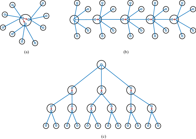
Figure 10: Merging GHZ states in various configurations. The arrows indicate CNOT gates, pointing from the source qubit to the target qubit. The target qubit is then measured in the Pauli-$Z$ basis. (a) Three GHZ states in a star configuration (Protocol 6). (b) Five GHZ states in a linear chain (Protocol 7). (c) 10 GHZ states in a tree configuration (Protocol 8).

E.1 Merging two GHZ states (Protocol 3)

Consider the following two GHZ states:

$$|\text{GHZ}_{n+1}\rangle_{A_{1}B_{1:n}} =\frac{1}{\sqrt{2}}\left(|0\rangle_{A_{1}}\otimes|0\rangle_{B_{1:n}}^{\otimes n}+|1\rangle_{A_{1}}\otimes|1\rangle_{B_{1:n}}^{\otimes n}\right),$$ (77)

$$|\text{GHZ}_{m+1}\rangle_{A_{2}C_{1:m}} =\frac{1}{\sqrt{2}}\left(|0\rangle_{A_{2}}\otimes|0\rangle_{C_{1:m}}^{\otimes m}+|1\rangle_{A_{2}}\otimes|1\rangle_{C_{1:m}}^{\otimes m}\right),$$ (78)

such that the qubits $A_{1}$ and $A_{2}$ are located at the same node. The protocol for merging these two states into a larger GHZ state is provided in Protocol 3.

Let us now prove that after executing Protocol 3 we deterministically have the GHZ state $|\text{GHZ}_{n+m+1}\rangle_{A_{1}B_{1:n}C_{1:m}}$ shared by $A_{1},B_{1},\dotsc,B_{n},C_{1},\dotsc,C_{m}$. First,

$$|\text{GHZ}_{n+1}\rangle\otimes|\text{GHZ}_{m+1}\rangle =\frac{1}{2}(|0\rangle_{A_{1}}\otimes|0\rangle_{A_{2}}\otimes|0\rangle_{B_{1}^{n}}^{\otimes n}\otimes|0\rangle_{C_{1}^{m}}^{\otimes m}$$

$$\qquad+|0\rangle_{A_{1}}\otimes|1\rangle_{A_{2}}\otimes|0\rangle_{B_{1}^{n}}^{\otimes n}\otimes|1\rangle_{C_{1}^{m}}^{\otimes m}$$

$$\qquad+|1\rangle_{A_{1}}\otimes|0\rangle_{A_{2}}\otimes|1\rangle_{B_{1}^{n}}^{\otimes n}\otimes|0\rangle_{C_{1}^{m}}^{\otimes m}$$

$$\qquad+|1\rangle_{A_{1}}\otimes|1\rangle_{A_{2}}\otimes|1\rangle_{B_{1}^{n}}^{\otimes n}\otimes|1\rangle_{C_{1}^{m}}^{\otimes m}).$$ (79)

Then, after the CNOT between $A_{1}$ and $A_{2}$, the state becomes

$$\frac{1}{2}(|0\rangle_{A_{1}}\otimes|0\rangle_{A_{2}}\otimes|0\rangle_{B_{1}^{n}}^{\otimes n}\otimes|0\rangle_{C_{1}^{m}}^{\otimes m}$$

$$\quad+|0\rangle_{A_{1}}\otimes|1\rangle_{A_{2}}\otimes|0\rangle_{B_{1}^{n}}^{\otimes n}\otimes|1\rangle_{C_{1}^{m}}^{\otimes m}$$

$$\quad+|1\rangle_{A_{1}}\otimes|1\rangle_{A_{2}}\otimes|1\rangle_{B_{1}^{n}}^{\otimes n}\otimes|0\rangle_{C_{1}^{m}}^{\otimes m}$$

$$\quad+|1\rangle_{A_{1}}\otimes|0\rangle_{A_{2}}\otimes|1\rangle_{B_{1}^{n}}^{\otimes n}\otimes|1\rangle_{C_{1}^{m}}^{\otimes m}).$$ (80)

From this, we can see immediately that, when $A_{2}$ measures its qubit in the $\{|0\rangle,|1\rangle\}$ basis, then the outcome “0” occurs with probability $\frac{1}{2}$, and the state conditioned on this outcome is

$$\frac{1}{\sqrt{2}}(|0\rangle_{A_{1}}\otimes|0\rangle_{B_{1}^{n}}^{\otimes n}\otimes|0\rangle_{C_{1}^{m}}^{\otimes m}+|1\rangle_{A_{1}}\otimes|1\rangle_{B_{1}^{n}}^{\otimes n}\otimes|1\rangle_{C_{1}^{m}}^{\otimes m})=|\text{GHZ}_{n+m+1}\rangle.$$ (81)

On the other hand, if the outcome “1” occurs, also with probability $\frac{1}{2}$, then the state conditioned on this outcome is

$$\frac{1}{\sqrt{2}}(|0\rangle_{A_{1}}\otimes|0\rangle_{B_{1}^{n}}^{\otimes n}\otimes|1\rangle_{C_{1}^{m}}^{\otimes m}+|1\rangle_{A_{1}}\otimes|1\rangle_{B_{1}^{n}}^{\otimes n}\otimes|0\rangle_{C_{1}^{m}}^{\otimes m}).$$ (82)

Thus, if $C_{1},C_{2},\dotsc,C_{m}$ apply the Pauli $X$ gate to their qubits, then we obtain the required GHZ state $|\text{GHZ}_{n+m+1}\rangle$. This completes the proof.

Remark 3.

Let us note that in Protocol 3, we merged the two GHZ states using the first two qubits, $A_{1}$ and $A_{2}$, of the two GHZ states. It is possible, however, to merge two GHZ states using any two qubits, one from each state, as long as both qubits belong to the same node. $\blacktriangleleft$

E.2 Merging GHZ states in a star topology

Protocol 3 generalizes to merging multiple (more than two) GHZ states in a star topology; see Fig. 10(a). It is analogous to Protocol 2. Consider $N\in\{2,3,\dotsc\}$ GHZ states, $|\text{GHZ}_{n_{1}+1}\rangle_{A_{1}B_{1:n_{1}}^{1}},|\text{GHZ}_{n_{2}+1}\rangle_{A_{1}B_{1:n_{2}}^{2}},\dotsc,|\text{GHZ}_{n_{N}+1}\rangle_{A_{N}B_{1:n_{N}}^{N}}$, such that the qubits $A_{i}$, $i\in\{1,2,\dotsc,N\}$, are located at the same node. The protocol for merging all of these GHZ states into the one large GHZ state $|\text{GHZ}_{1+N_{\text{tot}}}\rangle_{A_{1}B_{1:n_{1}}^{2}\dotsb B_{1:n_{N}}^{N}}$, with $N_{\text{tot}}=n_{1}+n_{2}+\dotsb+n_{N}$, is as follows.

Protocol 6 Merging GHZ states in a star topology

1:$N\in\{2,3,\dotsc\}$ GHZ states, $|\text{GHZ}_{n_{1}+1}\rangle_{A_{1}B_{1:n_{1}}^{1}},|\text{GHZ}_{n_{2}+1}\rangle_{A_{2}B_{1:n_{2}}^{2}},\dotsc,|\text{GHZ}_{n_{N}+1}\rangle_{A_{N}B_{1:n_{N}}^{N}}$, such that the qubits $A_{i}$, $i\in\{1,2,\dotsc,N\}$, are located at the same node.

2:GHZ state $|\text{GHZ}_{1+N_{\text{tot}}}\rangle_{A_{1}B_{1:n_{1}}^{2}\dotsb B_{1:n_{N}}^{N}}$, with $N_{\text{tot}}=n_{1}+n_{2}+\dotsb+n_{N}$.

3:Apply the gates $\text{CNOT}_{A_{1}A_{2}},\text{CNOT}_{A_{1}A_{3}},\dotsc,\text{CNOT}_{A_{1}A_{N}}$.

4:Measure each of the qubits $A_{2},A_{3},\dotsc,A_{N}$ in the basis $\{|0\rangle,|1\rangle\}$.

5:The outcome of measurement on $A_{2}$ is communicated to $B_{1:n_{2}}^{2}$, the outcome of measurement on $A_{3}$ is communicated to $B_{1:n_{3}}^{3}$, etc.

6:For every set $B_{1:n_{i}}^{i}$ of qubits, $i\in\{2,3,\dotsc,N\}$: if the outcome communicated by $A_{i}$ is 0, then do nothing; if the outcome communicated by $A_{i}$ is 1, then apply the Pauli-$X$ gate to all qubits $B_{1:n_{i}}^{i}$.

The number of gates needed in Protocol 6 is the number of CNOT gates in the first step, which is $N-1$.

We can verify that Protocol 6 works as claimed. The initial state is

$$\bigotimes_{j=1}^{N}|\text{GHZ}_{n_{j}+1}\rangle_{A_{j}B_{1:n_{j}}^{j}}=\frac{1}{\sqrt{2^{N}}}\left(\sum_{x_{1}\in\{0,1\}}|x_{1}\rangle_{A_{1}}\otimes|x_{1}\rangle_{B_{1:n_{1}}^{1}}^{\otimes n_{1}}\right)\otimes\left(\sum_{x_{2}\in\{0,1\}}|x_{2}\rangle_{A_{2}}\otimes|x_{2}\rangle_{B_{1:n_{2}}^{2}}^{\otimes n_{2}}\right)\otimes\dotsb\\ \otimes\left(\sum_{x_{N}\in\{0,1\}}|x_{N}\rangle_{A_{N}}\otimes|x_{N}\rangle_{B_{1:n_{N}}^{N}}^{\otimes n_{N}}\right).$$ (83)

After the CNOT gates $\text{CNOT}_{A_{1}A_{2}},\text{CNOT}_{A_{1}A_{3}},\dotsc,\text{CNOT}_{A_{1}A_{N}}$, we obtain the state

$$\frac{1}{\sqrt{2^{N}}}\sum_{x_{1},x_{2},\dotsc,x_{N}\in\{0,1\}}|x_{1}\rangle_{A_{1}}\otimes|x_{1}\rangle_{B_{1:n_{1}}^{1}}^{\otimes n_{1}}\otimes|x_{1}\oplus x_{2}\rangle_{A_{2}}\otimes|x_{2}\rangle_{B_{1:n_{2}}^{2}}^{\otimes n_{2}}\otimes\dotsb\otimes|x_{1}\oplus x_{N}\rangle_{A_{N}}\otimes|x_{n_{N}}\rangle_{B_{1:n_{N}}^{N}}^{\otimes n_{N}}.$$ (84)

Then, for every collection $(y_{1},y_{2},\dotsc,y_{N-1})\in\{0,1\}^{N-1}$ of measurement outcomes corresponding to the $Z$-basis measurement of the qubits $A_{2},A_{3},\dotsc,A_{N}$, we obtain the state

$$\frac{1}{\sqrt{2}}\sum_{x_{1},x_{2},\dotsc,x_{N}\in\{0,1\}^{N}}|x_{1}\rangle_{A_{1}}\otimes|x_{1}\rangle_{B_{1:n_{1}}^{1}}^{\otimes n_{1}}\otimes\langle y_{1}|x_{1}\oplus x_{2}\rangle|x_{2}\rangle_{B_{1:n_{2}}^{2}}^{\otimes n_{2}}\otimes\dotsb\otimes\langle y_{N-1}|x_{1}\oplus x_{N}\rangle|x_{N}\rangle_{B_{1:n_{N}}^{N}}^{\otimes n_{N}}$$ (85)

$$\quad=\sum_{x_{1}\in\{0,1\}}|x_{1}\rangle_{A_{1}}\otimes|x_{1}\rangle_{B_{1:n_{1}}^{1}}^{\otimes n_{1}}\otimes|x_{1}\oplus y_{1}\rangle_{B_{1:n_{2}}^{2}}^{\otimes n_{2}}\otimes\dotsb\otimes|x_{1}\oplus y_{N-1}\rangle_{B_{1:n_{N}}^{N}}^{\otimes n_{N}}$$ (86)

$$\quad=\left(\mathbbm{1}_{A_{1}B_{1:n_{1}}^{1}}\otimes(X^{y_{1}})_{B_{1:n_{2}}^{2}}^{\otimes n_{2}}\otimes\dotsb\otimes(X^{y_{N-1}})_{B_{1:n_{N}}^{N}}^{\otimes n_{N}}\right)|\text{GHZ}_{1+N_{\text{tot}}}\rangle_{A_{1}B_{1:n_{1}}\dotsb B_{1:n_{N}}},$$ (87)

as required.

We can write down the action of Protocol 6 as an LOCC channel as follows:

$$\mathcal{L}\!\left(\rho_{A_{1}B_{1:n_{1}}^{1}A_{2}B_{1:n_{2}}^{2}\dotsb A_{N}B_{1:n_{N}}^{N}}\right)=\sum_{\vec{y}\in\{0,1\}}\left(\langle\vec{y}|_{A_{2:N}}\text{CNOT}_{N}\otimes(X^{y_{1}})_{B_{1:n_{2}}^{2}}^{\otimes n_{2}}\otimes\dotsb\otimes(X^{y_{N-1}})_{B_{1:n_{N}}^{N}}^{\otimes n_{N}}\right)\rho_{A_{1}B_{1:n_{1}}^{1}A_{2}B_{1:n_{2}}^{2}\dotsb A_{N}B_{1:n_{N}}^{N}}\\ \times\left(\text{CNOT}_{N}|\vec{y}\rangle_{A_{2:N}}\otimes(X^{y_{1}})_{B_{1:n_{2}}^{2}}^{\otimes n_{2}}\otimes\dotsb\otimes(X^{y_{N-1}})_{B_{1:n_{N}}^{N}}^{\otimes n_{N}}\right),$$ (88)

where $\rho_{A_{1}B_{1:n_{1}}^{1}A_{2}B_{1:n_{2}}^{2}\dotsb A_{N}B_{1:n_{N}}^{N}}$ is an arbitrary state, and we recall the definition of $\text{CNOT}_{N}$ from (29).

E.2.1 Proof of Theorem 10

Here, we provide an expression for the fidelity of the state after Protocol 6 with respect to the GHZ state, when the input states are noisy. This then provides a proof of Theorem 10 as a special case when $N=2$.

Proposition 13.

Consider states $\rho_{A_{1}B_{1:n_{1}}^{1}}^{1},\rho_{A_{2}B_{1:n_{2}}^{2}}^{2},\dotsc,\rho_{A_{N}B_{1:n_{N}}^{N}}^{N}$, representing noisy input states to Protocol 6. With these input states, the fidelity of the state produced by Protocol 6 with respect to the final, ideal GHZ state is

$$\langle\text{GHZ}_{1+N_{\text{tot}}}|\mathcal{L}\!\left(\rho_{A_{1}B_{1:n_{1}}^{1}}^{1}\otimes\rho_{A_{2}B_{1:n_{2}}^{2}}^{2}\otimes\dotsb\rho_{A_{N}B_{1:n_{N}}^{N}}^{N}\right)|\text{GHZ}_{1+N_{\text{tot}}}\rangle$$

$$\quad=\sum_{\vec{z}\in\{0,1\}^{N-1}}\langle\text{GHZ}_{n_{1}+1}^{(z^{\prime},\vec{0})}|\rho_{A_{1}B_{1:n_{1}}^{1}}^{1}|\text{GHZ}_{n_{1}+1}^{(z^{\prime},\vec{0})}\rangle\langle\text{GHZ}_{n_{2}+1}^{(z_{1},\vec{0})}|\rho_{A_{2}B_{1:n_{2}}^{2}}^{2}|\text{GHZ}_{n_{2}+1}^{(z_{1},\vec{0})}\rangle\dotsb\langle\text{GHZ}_{n_{N}+1}^{(z_{N-1},\vec{0})}|\rho_{A_{N}B_{1:n_{N}}^{N}}^{N}|\text{GHZ}_{n_{N}+1}^{(z_{N-1},\vec{0})}\rangle,$$ (89)

$z^{\prime}=z_{1}\oplus z_{2}\oplus\dotsb\oplus z_{N-1}$, and we have introduced the following $n$-qubit GHZ basis, for $n\in\{2,3,\dotsc\}$:

$$|\text{GHZ}_{n}^{(z,\vec{x})}\rangle\coloneqq(Z^{z}\otimes X^{\vec{x}})|\text{GHZ}_{n}\rangle,$$ (90)

with $z\in\{0,1\}$ and $\vec{x}\in\{0,1\}^{n-1}$.

Remark 4.

It is straightforward to verify that the state vectors in (90) form an orthonormal basis for the vector space $(\mathbb{C}^{2})^{\otimes n}$ corresponding to $n$ qubits. (Note that for $n=2$, these state vectors form the two-qubit Bell basis.) $\blacktriangleleft$

Proof.

We start by defining

$$|w(\vec{y})\rangle \coloneqq\left(\text{CNOT}_{N}|\vec{y}\rangle_{A_{2:N}}\otimes(X^{y_{1}})_{B_{1:n_{2}}^{2}}^{\otimes n_{2}}\otimes\dotsb\otimes(X^{y_{N-1}})_{B_{1:n_{N}}^{N}}^{\otimes n_{N}}\right)|\text{GHZ}_{1+N_{\text{tot}}}\rangle_{A_{1}B_{1:n_{1}}^{1}B_{1:n_{2}}^{2}\dotsb B_{1:n_{N}}^{N}}$$ (91)

$$=\frac{1}{\sqrt{2}}\sum_{x\in\{0,1\}}\text{CNOT}_{N}|x\rangle_{A_{1}}|\vec{y}\rangle_{A_{2:N}}\otimes|x\rangle_{B_{1:n_{1}}^{1}}^{\otimes n_{1}}\otimes(X^{y_{1}})_{B_{1:n_{2}}^{2}}^{\otimes n_{2}}|x\rangle_{B_{1:n_{2}}^{2}}^{\otimes n_{2}}\otimes\dotsb\otimes(X^{y_{N-1}})_{B_{1:n_{N}}^{N}}^{\otimes n_{N}}|x\rangle_{B_{1:n_{N}}^{N}}^{\otimes n_{N}}$$ (92)

$$=\frac{1}{\sqrt{2}}\sum_{x\in\{0,1\}}|x\rangle_{A_{1}}|y_{1}\oplus x\rangle_{A_{2}}\dotsb|y_{N-1}\oplus x\rangle_{A_{N}}\otimes|x\rangle_{B_{1:n_{1}}^{1}}^{\otimes n_{1}}\otimes|y_{1}\oplus x\rangle_{B_{1:n_{2}}^{2}}^{\otimes n_{2}}\otimes\dotsb\otimes|y_{N-1}\oplus x\rangle_{B_{1:n_{N}}}^{\otimes n_{N}}$$ (93)

$$=\frac{1}{\sqrt{2}}\sum_{x\in\{0,1\}}|x\rangle_{A_{1}}|x\rangle_{B_{1:n_{1}}}^{\otimes n_{1}}\otimes|y_{1}\oplus x\rangle_{A_{2}}|y_{1}\oplus x\rangle_{B_{1:n_{2}}^{2}}^{\otimes n_{2}}\otimes\dotsb\otimes|y_{N-1}\oplus x\rangle_{A_{N}}|y_{N-1}\oplus x\rangle_{B_{1:n_{N}}^{N}}^{\otimes n_{N}}.$$ (94)

Now, it is straightforward to show that

$$|x\rangle^{\otimes n}=\frac{1}{\sqrt{2}}\sum_{z\in\{0,1\}}(-1)^{zx}|\text{GHZ}_{n}^{(z,\vec{0})}\rangle,$$ (95)

for $x\in\{0,1\}$. With this, we find that

$$|w(\vec{y})\rangle =\frac{1}{\sqrt{2}}\sum_{x\in\{0,1\}}\left(\frac{1}{\sqrt{2}}\sum_{z_{1}\in\{0,1\}}(-1)^{z_{1}x}|\text{GHZ}_{n_{1}+1}^{(z_{1},\vec{0})}\rangle_{A_{1}B_{1:n_{1}}^{1}}\right)\otimes\left(\frac{1}{\sqrt{2}}\sum_{z_{2}\in\{0,1\}}(-1)^{z_{2}(y_{1}\oplus x)}|\text{GHZ}_{n_{2}+1}^{(z_{2},\vec{0})}\rangle_{A_{2}B_{1:n_{2}}^{2}}\right)\otimes\dotsb$$

$$\qquad\qquad\qquad\qquad\dotsb\otimes\left(\frac{1}{\sqrt{2}}\sum_{z_{N}\in\{0,1\}}(-1)^{z_{N}(y_{N-1}\oplus x)}|\text{GHZ}_{n_{N}+1}^{(z_{N},\vec{0})}\rangle_{A_{N}B_{1:n_{N}}^{N}}\right)$$ (96)

$$=\frac{1}{\sqrt{2^{N+1}}}\sum_{z_{1},z_{2},\dotsc,z_{N}\in\{0,1\}}(-1)^{z_{2}y_{1}+z_{3}y_{2}+\dotsb+z_{N}y_{N-1}}\underbrace{\left(\sum_{x\in\{0,1\}}(-1)^{x(z_{1}\oplus z_{2}\oplus\dotsb\oplus z_{N})}\right)}_{2\delta_{z_{1},z_{2}\oplus\dotsb\oplus z_{N}}}$$

$$\qquad\qquad\qquad\qquad\times|\text{GHZ}_{n_{1}+1}^{(z_{1},\vec{0})}\rangle_{A_{1}B_{1:n_{1}}^{1}}\otimes|\text{GHZ}_{n_{2}+1}^{(z_{2},\vec{0})}\rangle_{A_{2}B_{1:n_{2}}^{2}}\otimes\dotsb\otimes|\text{GHZ}_{n_{N}+1}^{(z_{N},\vec{0})}\rangle_{A_{N}B_{1:n_{N}}^{N}}$$ (97)

$$=\frac{1}{\sqrt{2^{N-1}}}\sum_{z_{2},z_{3},\dotsc,z_{N}\in\{0,1\}}(-1)^{z_{2}y_{1}+z_{3}y_{2}+\dotsb+z_{N}y_{N-1}}|\text{GHZ}_{n_{1}+1}^{(z^{\prime},\vec{0})}\rangle_{A_{1}B_{1:n_{1}}^{1}}\otimes|\text{GHZ}_{n_{2}+1}^{(z_{2},\vec{0})}\rangle_{A_{2}B_{1:n_{2}}^{2}}\otimes\dotsb\otimes|\text{GHZ}_{n_{N}+1}^{(z_{N},\vec{0})}\rangle_{A_{N}B_{1:n_{N}}^{N}},$$ (98)

where in the final line we let $z^{\prime}=z_{2}\oplus z_{3}\oplus\dotsb\oplus z_{N}$. Therefore, the fidelity of the state in (88) is given by

$$\langle\text{GHZ}_{1+N_{\text{tot}}}|\mathcal{L}\!\left(\rho_{A_{1}B_{1:n_{1}}^{1}A_{2}B_{1:n_{2}}^{2}\dotsb A_{N}B_{1:n_{N}}^{N}}\right)|\text{GHZ}_{1+N_{\text{tot}}}\rangle$$

$$\quad=\sum_{\vec{y}\in\{0,1\}^{N-1}}\langle w(\vec{y})|\rho_{A_{1}B_{1:n_{1}}^{1}A_{2}B_{1:n_{2}}^{2}\dotsb A_{N}B_{1:n_{N}}^{N}}|w(\vec{y})\rangle$$ (99)

$$\quad=\frac{1}{2^{N-1}}\sum_{\vec{y},\vec{z},\vec{w}\in\{0,1\}^{N-1}}(-1)^{\vec{z}\cdot\vec{y}}(-1)^{\vec{w}\cdot\vec{y}}\left(\langle\text{GHZ}_{n_{1}+1}^{(z^{\prime},\vec{0})}|_{A_{1}B_{1:n_{1}}^{1}}\otimes\langle\text{GHZ}_{n_{2}+1}^{(z_{1},\vec{0})}|_{A_{2}B_{1:n_{2}}^{2}}\otimes\dotsb\otimes\langle\text{GHZ}_{n_{N}+1}^{(z_{N},\vec{0})}|_{A_{N}B_{1:n_{N}}^{N}}\right)$$

$$\qquad\qquad\times\rho_{A_{1}B_{1:n_{1}}^{1}A_{2}B_{1:n_{2}}^{2}\dotsb A_{N}B_{1:n_{N}}^{N}}\left(|\text{GHZ}_{n_{1}+1}^{(w^{\prime},\vec{0})}\rangle_{A_{1}B_{1:n_{1}}^{1}}\otimes|\text{GHZ}_{n_{2}+1}^{(w_{1},\vec{0})}\rangle_{A_{2}B_{1:n_{2}}^{2}}\otimes\dotsb\otimes|\text{GHZ}_{n_{N}+1}^{(w_{N},\vec{0})}\rangle_{A_{N}B_{1:n_{N}}^{N}}\right)$$ (100)

$$\quad=\sum_{\vec{z}\in\{0,1\}^{N-1}}\left(\langle\text{GHZ}_{n_{1}+1}^{(z^{\prime},\vec{0})}|_{A_{1}B_{1:n_{1}}^{1}}\otimes\langle\text{GHZ}_{n_{2}+1}^{(z_{1},\vec{0})}|_{A_{2}B_{1:n_{2}}^{2}}\otimes\dotsb\otimes\langle\text{GHZ}_{n_{N}+1}^{(z_{N},\vec{0})}|_{A_{N}B_{1:n_{N}}^{N}}\right)$$

$$\qquad\qquad\times\rho_{A_{1}B_{1:n_{1}}^{1}A_{2}B_{1:n_{2}}^{2}\dotsb A_{N}B_{1:n_{N}}^{N}}\left(|\text{GHZ}_{n_{1}+1}^{(z^{\prime},\vec{0})}\rangle_{A_{1}B_{1:n_{1}}^{1}}\otimes|\text{GHZ}_{n_{2}+1}^{(z_{1},\vec{0})}\rangle_{A_{2}B_{1:n_{2}}^{2}}\otimes\dotsb\otimes|\text{GHZ}_{n_{N}+1}^{(z_{N},\vec{0})}\rangle_{A_{N}B_{1:n_{N}}^{N}}\right),$$ (101)

as required.  $\blacksquare$

E.3 Merging GHZ states in a linear topology

Merging GHZ states in a linear topology (see Fig. 10(b)) proceeds similarly, as we outline in Protocol 7.

Protocol 7 Merging GHZ states in a linear topology

1:$N\in\{2,3,\dotsc\}$ GHZ states, $|\text{GHZ}_{n_{1}+1}\rangle_{A_{1:n_{1}}^{1}R_{1}},\,|\text{GHZ}_{n_{2}+2}\rangle_{R_{2}A_{1:n_{2}}^{2}R_{3}},\dotsc,|\text{GHZ}_{n_{N-1}+2}\rangle_{R_{2N-4}A_{1:n_{N-1}}^{N-1}R_{2N-3}},\,|\text{GHZ}_{n_{N}+1}\rangle_{R_{2N-2}A_{1:n_{N}}^{N}}$, such that the qubits $R_{i}$ and $R_{i+1}$, $i\in\{1,3,5,\dotsc,2N-1\}$, are located at the same node; see Fig. 10(b).

2:GHZ state $|\text{GHZ}_{N_{\text{tot}}}\rangle$, with $N_{\text{tot}}=n_{1}+n_{2}+\dotsb+n_{N}+N-1$, shared by $A_{1:n_{1}}^{1},R_{1},A_{1:n_{2}}^{2},R_{3},\dotsc,A_{1:n_{N-1}}^{N-1},R_{2N-3},A_{1:n_{N}}^{N}$.

3:Apply the CNOT gates $\text{CNOT}_{R_{i}R_{i+1}}$, $i\in\{1,3,5,\dotsc,2N-3\}$.

4:Measure the target qubits $R_{2},R_{4},R_{6},\dotsc,R_{2N-2}$ in the $Z$-basis $\{|0\rangle,|1\rangle\}$. The outcomes $z_{1},z_{2},\dotsc,z_{N-1}\in\{0,1\}$ are communicated to all nodes.

5:The qubits associated with the second GHZ state apply the Pauli-$X$ correction $X^{z_{1}}$; the qubits associated with the third GHZ state apply the Pauli-$X$ correction $X^{z_{1}\oplus z_{2}}$; etc. In general, the qubits associated with the $k$-th node, $k\in\{2,3,\dotsc,N\}$, apply the Pauli-$X$ correction $X^{z_{1}\oplus z_{2}\oplus\dotsb\oplus z_{k-1}}$.

Let us verify that Protocol 7 performs as expected. The initial state is

$$|\text{GHZ}_{n_{1}+1}\rangle_{A_{1:n_{1}}^{1}R_{1}}\otimes|\text{GHZ}_{n_{2}+2}\rangle_{R_{2}A_{1:n_{2}}^{2}R_{3}}\otimes|\text{GHZ}_{n_{3}+2}\rangle_{R_{4}A_{1:n_{3}}^{3}R_{5}}\dotsb\otimes|\text{GHZ}_{n_{N-1}+2}\rangle_{R_{2N-4}A_{1:n_{N-1}}^{N-1}R_{2N-3}}\otimes|\text{GHZ}_{n_{N}+1}\rangle_{R_{2N-2}A_{1:n_{N}}^{N}}\\ =\frac{1}{\sqrt{2^{N}}}\sum_{x_{1},x_{2},x_{3},\dotsc,x_{N-1},x_{N}\in\{0,1\}}|x_{1}\rangle_{A_{1:n_{1}}^{1}}^{\otimes n_{1}}|x_{1}\rangle_{R_{1}}\otimes|x_{2}\rangle_{R_{2}}|x_{2}\rangle_{A_{1:n_{2}}^{2}}^{\otimes n_{2}}|x_{2}\rangle_{R_{3}}\otimes|x_{3}\rangle_{R_{4}}|x_{3}\rangle_{A_{1:n_{3}}}^{\otimes n_{3}}|x_{3}\rangle_{R_{5}}\otimes\dotsb\\ \dotsb\otimes|x_{N-1}\rangle_{R_{2N-4}}|x_{N-1}\rangle_{A_{1:n_{N-1}}^{N-1}}^{\otimes n_{N-1}}|x_{N-1}\rangle_{R_{2N-3}}\otimes|x_{N}\rangle_{R_{2N-2}}|x_{N}\rangle_{A_{1:n_{N}}^{N}}^{\otimes n_{N}}.$$ (102)

After the CNOT gates, we obtain

$$\frac{1}{\sqrt{2^{N}}}\sum_{x_{1},x_{2},x_{3},\dotsc,x_{N-1},x_{N}\in\{0,1\}}|x_{1}\rangle_{A_{1:n_{1}}^{1}}^{\otimes n_{1}}|x_{1}\rangle_{R_{1}}\otimes|x_{1}\oplus x_{2}\rangle_{R_{2}}|x_{2}\rangle_{A_{1:n_{2}}^{2}}^{\otimes n_{2}}|x_{2}\rangle_{R_{3}}\otimes|x_{2}\oplus x_{3}\rangle_{R_{4}}|x_{3}\rangle_{A_{1:n_{3}}^{3}}^{\otimes n_{3}}|x_{3}\rangle_{R_{5}}\otimes\dotsb\\ \dotsb\otimes|x_{N-2}\oplus x_{N-1}\rangle_{R_{2N-4}}|x_{N-1}\rangle_{A_{1:n_{N-1}}^{N-1}}^{\otimes n_{N-1}}|x_{N-1}\rangle_{R_{2N-3}}\otimes|x_{N-1}\oplus x_{N}\rangle_{R_{2N-2}}|x_{N}\rangle_{A_{1:n_{N}}^{N}}^{\otimes n_{N}}.$$ (103)

Then, upon measuring the target qubits $R_{2},R_{4},\dotsc$ in the $\{|0\rangle,|1\rangle\}$ basis, to every outcome string $(z_{1},z_{2},\dotsc,z_{N-1})\in\{0,1\}^{N-1}$ we have the following associated (unnormalized) post-measurement state:

$$\frac{1}{\sqrt{2^{N}}}\sum_{x_{1},x_{2},x_{3},\dotsc,x_{N-1},x_{N}\in\{0,1\}}|x_{1}\rangle_{A_{1:n_{1}}^{1}}^{\otimes n_{1}}|x_{1}\rangle_{R_{1}}\otimes\langle z_{1}|x_{1}\oplus x_{2}\rangle_{R_{2}}|x_{2}\rangle_{A_{1:n_{2}}^{2}}^{\otimes n_{2}}|x_{2}\rangle_{R_{3}}\otimes\langle z_{2}|x_{2}\oplus x_{3}\rangle_{R_{4}}|x_{3}\rangle_{A_{1:n_{3}}^{3}}^{\otimes n_{3}}|x_{3}\rangle_{R_{5}}\otimes\dotsb\\ \dotsb\otimes\langle z_{N-2}|x_{N-2}\oplus x_{N-1}\rangle_{R_{2N-4}}|x_{N-1}\rangle_{A_{1:n_{N-1}}^{N-1}}^{\otimes n_{N-1}}|x_{N-1}\rangle_{R_{2N-3}}\otimes\langle z_{N-1}|x_{N-1}\oplus x_{N}\rangle_{R_{2N-2}}|x_{N}\rangle_{A_{1:n_{N}}^{N}}^{\otimes n_{N}},$$ (104)

which we can simplify to

$$\frac{1}{\sqrt{2^{N}}}\sum_{x_{1}\in\{0,1\}}|x_{1}\rangle_{A_{1:n_{1}}^{1}}^{\otimes n_{1}}|x_{1}\rangle_{R_{1}}\otimes|z_{1}\oplus x_{1}\rangle_{A_{1:n_{2}}^{2}}^{\otimes n_{2}}|z_{1}\oplus x_{1}\rangle_{R_{3}}\otimes|z_{1}\oplus z_{2}\oplus x_{1}\rangle_{A_{1:n_{3}}^{3}}^{\otimes n_{3}}|z_{1}\oplus z_{2}\oplus x_{1}\rangle_{R_{5}}\otimes\dotsb\\ \dotsb\otimes|z_{1}\oplus z_{2}\oplus\dotsb\oplus z_{N-2}\oplus x_{1}\rangle_{A_{1:n_{N-1}}^{N-1}}^{\otimes n_{N-1}}|z_{1}\oplus z_{2}\oplus\dotsb\oplus z_{N-2}\oplus x_{1}\rangle_{R_{2N-3}}\otimes|z_{1}\oplus z_{2}\oplus\dotsb\oplus z_{N-1}\oplus x_{1}\rangle_{A_{1:n_{N}}^{N}}^{\otimes n_{N}}\\ =\left((X^{z_{1}})_{A_{1:n_{2}}^{2}R_{3}}^{\otimes(n_{2}+1)}\otimes(X^{z_{1}\oplus z_{2}})_{A_{1:n_{3}}^{3}R_{5}}^{\otimes(n_{3}+1)}\otimes\dotsb\otimes(X^{z_{1}\oplus z_{2}\oplus\dotsb\oplus z_{N-2}})_{A_{1:n_{N-1}}^{N-1}R_{2N-3}}^{\otimes(n_{N-1}+1)}\otimes(X^{z_{1}\oplus z_{2}\oplus\dotsb\oplus z_{N-1}})_{A_{1:n_{N}}^{N}}^{\otimes n_{N}}\right)|\text{GHZ}_{N_{\text{tot}}}\rangle.$$ (105)

We thus see that, as expected, the resulting state is the required GHZ state up to the appropriate Pauli-$X$ corrections.

As an LOCC channel, we can write the action of Protocol 7 as follows:

$$\mathcal{L}\left(\rho_{A_{1:n_{1}}^{1}R_{1}R_{2}A_{1:n_{2}}^{2}R_{3}\dotsb R_{2N-4}A_{1:n_{N-1}}^{N-1}R_{2N-3}R_{2N-2}A_{1:n_{N}}^{N}}\right)\\ =\sum_{\vec{z}\in\{0,1\}^{N-1}}\left((X^{y_{1}})_{A_{1:n_{2}}^{2}R_{3}}^{\otimes(n_{2}+1)}\otimes(X^{y_{2}})_{A_{1:n_{3}}^{3}R_{5}}^{\otimes(n_{3}+1)}\otimes\dotsb\otimes(X^{y_{N-2}})_{A_{1:n_{N-1}}^{N-1}R_{2N-3}}^{\otimes(n_{N-1}+1)}\otimes(X^{y_{N-1}})_{A_{1:n_{N}}^{N}}^{\otimes n_{N}}\right)\\ \times\left(\langle\vec{z}|_{R_{2}R_{4}R_{6}\dotsb R_{2N-2}}\text{CNOT}_{N}^{\prime}\right)\rho_{A_{1:n_{1}}^{1}R_{1}R_{2}A_{1:n_{2}}^{2}R_{3}\dotsb R_{2N-4}A_{1:n_{N-1}}^{N-1}R_{2N-3}R_{2N-2}A_{1:n_{N}}^{N}}\left(\text{CNOT}_{N}^{\prime}|\vec{z}\rangle_{R_{2}R_{4}R_{6}\dotsb R_{2N-2}}\right)\\ \times\left((X^{y_{1}})_{A_{1:n_{2}}^{2}R_{3}}^{\otimes(n_{2}+1)}\otimes(X^{y_{2}})_{A_{1:n_{3}}^{3}R_{5}}^{\otimes(n_{3}+1)}\otimes\dotsb\otimes(X^{y_{N-2}})_{A_{1:n_{N-1}}^{N-1}R_{2N-3}}^{\otimes(n_{N-1}+1)}\otimes(X^{y_{N-1}})_{A_{1:n_{N}}^{N}}^{\otimes n_{N}}\right),$$ (106)

where

$$y_{k} \coloneqq z_{1}\oplus z_{2}\oplus\dotsb\oplus z_{k},\quad k\in\{1,2,\dotsc,N-1\},$$ (107)

$$\text{CNOT}_{N}^{\prime} \coloneqq\text{CNOT}_{R_{1}R_{2}}\text{CNOT}_{R_{3}R_{4}}\dotsb\text{CNOT}_{R_{2N-3}R_{2N-2}}.$$ (108)

Proposition 14.

Consider states $\rho_{A_{1:n_{1}}^{1}R_{1}}^{1},\rho_{R_{2}A_{1:n_{2}}^{2}R_{3}}^{2},\dotsc,\rho_{R_{2N-2}A_{1:n_{N}}^{N}}^{N}$, representing noisy input states to Protocol 7. With these input states, the fidelity of the state produced by Protocol 7 with respect to the final, ideal GHZ state is

$$\langle\text{GHZ}_{N_{\text{tot}}}|\mathcal{L}\!\left(\rho_{A_{1:n_{1}}^{1}R_{1}}^{1}\otimes\rho_{R_{2}A_{1:n_{2}}^{2}R_{3}}^{2}\otimes\dotsb\otimes\rho_{R_{2N-2}A_{1:n_{N}}^{N}}^{N}\right)\\ =\sum_{y_{1},y_{2},\dotsc,y_{N-1}\in\{0,1\}}\langle\text{GHZ}_{n_{1}+1}^{(y_{1},\vec{0})}|\rho_{A_{1:n_{1}}^{1}R_{1}}^{1}|\text{GHZ}_{n_{1}+1}^{(y_{1},\vec{0})}\rangle\langle\text{GHZ}_{n_{2}+2}^{(y_{2},\vec{0})}|\rho_{R_{2}A_{1:n_{2}}^{2}R_{3}}^{2}|\text{GHZ}_{n_{2}+2}^{(y_{2},\vec{0})}\rangle\dotsb\\ \dotsb\langle\text{GHZ}_{n_{N}+1}^{(y^{\prime},\vec{0})}|\rho_{R_{2N-2}A_{1:n_{N}}}^{N}|\text{GHZ}_{n_{N}+1}^{(y^{\prime},\vec{0})}\rangle_{R_{2N-2}A_{1:n_{N}}},$$ (109)

where $y^{\prime}=y_{1}\oplus y_{2}\oplus\dotsb\oplus y_{N-1}$.

Proof.

We start by defining the vector

$$|u(\vec{z})\rangle\coloneqq\left(\text{CNOT}_{N}^{\prime}|\vec{z}\rangle_{R_{2}R_{4}R_{6}\dotsb R_{2N-2}}\right)\left((X^{y_{1}})_{A_{1:n_{2}}^{2}R_{3}}^{\otimes(n_{2}+1)}\otimes(X^{y_{2}})_{A_{1:n_{3}}^{3}R_{5}}^{\otimes(n_{3}+1)}\otimes\dotsb\right.\\ \left.\dotsb\otimes(X^{y_{N-2}})_{A_{1:n_{N-1}}^{N-1}R_{2N-3}}^{\otimes(n_{N-1}+1)}\otimes(X^{y_{N-1}})_{A_{1:n_{N}}^{N}}^{\otimes n_{N}}\right)|\text{GHZ}_{N_{\text{tot}}}\rangle_{A_{1:n_{1}}^{1}R_{1}A_{1:n_{2}}^{2}R_{3}\dotsb A_{1:n_{N-1}}^{N-1}R_{2N-3}A_{1:n_{N}}^{N}},$$ (110)

which can be simplified as follows:

$$|u(\vec{z})\rangle =\frac{1}{\sqrt{2}}\sum_{\vec{x}\in\{0,1\}}|x\rangle_{A_{1:n_{1}}^{1}}^{\otimes n_{1}}\text{CNOT}_{R_{1}R_{2}}|x,z_{1}\rangle_{R_{1}R_{2}}\otimes(X^{y_{1}}|x\rangle)_{A_{1:n_{2}}^{2}}^{\otimes n_{2}}\text{CNOT}_{R_{3}R_{4}}X_{R_{3}}^{y_{1}}|x,z_{2}\rangle_{R_{3}R_{4}}\otimes(X^{y_{2}}|x\rangle)_{A_{1:n_{3}}^{3}}^{\otimes n_{3}}\text{CNOT}_{R_{5}R_{6}}X_{R_{5}}^{y_{2}}|x,z_{3}\rangle_{R_{5}R_{6}}\otimes\dotsb$$

$$\qquad\qquad\dotsb\otimes(X^{y_{N-2}}|x\rangle)_{A_{1:n_{N-1}}^{N-1}}^{\otimes n_{N-1}}\text{CNOT}_{R_{2N-3}R_{2N-2}}X_{R_{2N-3}}^{y_{N-2}}|x,z_{N-1}\rangle_{R_{2N-3}R_{2N-2}}(X^{y_{N-1}}|x\rangle)_{A_{1:n_{N}}}^{\otimes n_{N}}$$ (111)

$$=\frac{1}{\sqrt{2}}\sum_{x\in\{0,1\}}|x\rangle_{A_{1:n_{1}}}^{\otimes n_{1}}|x\rangle_{R_{1}}\otimes|x\oplus z_{1}\rangle_{R_{2}}|x\oplus y_{1}\rangle_{A_{1:n_{2}}^{2}}^{\otimes n_{2}}|x\oplus y_{1}\rangle_{R_{3}}\otimes|x\oplus y_{1}\oplus z_{2}\rangle_{R_{4}}|x\oplus y_{2}\rangle_{A_{1:n_{3}}^{3}}^{\otimes n_{3}}|x\oplus y_{2}\rangle_{R_{5}}|x\oplus y_{2}\oplus z_{3}\rangle_{R_{6}}\otimes\dotsb$$

$$\qquad\qquad\dotsb\otimes|x\oplus y_{N-2}\rangle_{A_{1:n_{N-1}}^{N-1}}^{\otimes n_{N-1}}|x\oplus y_{N-2}\rangle_{R_{2N-3}}\otimes|x\oplus y_{N-2}\oplus z_{N-1}\rangle_{R_{2N-2}}|x\oplus y_{N-1}\rangle_{A_{1:n_{N}}^{N}}^{\otimes n_{N}}$$ (112)

$$=\frac{1}{\sqrt{2}}\sum_{x\in\{0,1\}}|x\rangle_{A_{1:n_{1}}}^{\otimes n_{1}}|x\rangle_{R_{1}}\otimes|x\oplus z_{1}\rangle_{R_{2}}|x\oplus z_{1}\rangle_{A_{1:n_{2}}^{2}}^{\otimes n_{2}}|x\oplus z_{1}\rangle_{R_{3}}\otimes|x\oplus z_{1}\oplus z_{2}\rangle_{R_{4}}|x\oplus z_{1}\oplus z_{2}\rangle_{A_{1:n_{3}}^{3}}^{\otimes n_{3}}|x\oplus z_{1}\oplus z_{2}\rangle_{R_{5}}$$

$$\qquad\qquad\otimes|x\oplus z_{1}\oplus z_{2}\oplus z_{3}\rangle_{R_{6}}\otimes\dotsb\otimes|x\oplus z_{1}\oplus\dotsb\oplus z_{N-2}\rangle_{A_{1:n_{N-1}}^{N-1}}^{\otimes n_{N-1}}|x\oplus z_{1}\oplus\dotsb\oplus z_{N-2}\rangle_{R_{2N-3}}$$

$$\qquad\qquad\otimes|x\oplus z_{1}\oplus\dotsb\oplus z_{N-2}\oplus z_{N-1}\rangle_{R_{2N-2}}|x\oplus z_{1}\oplus\dotsb\oplus z_{N-1}\rangle_{A_{1:n_{N}}^{N}}^{\otimes n_{N}},$$ (113)

where we have used (107) and (108). Let us now use (95) to make further simplifications, as follows:

$$|u(\vec{z})\rangle =\frac{1}{\sqrt{2}}\frac{1}{\sqrt{2^{N}}}\sum_{x\in\{0,1\}}\sum_{y_{1},y_{2},\dotsc,y_{N}\in\{0,1\}}(-1)^{xy_{1}}|\text{GHZ}_{n_{1}+1}^{(y_{1},\vec{0})}\rangle_{A_{1:n_{1}}^{1}R_{1}}\otimes(-1)^{(x\oplus z_{1})y_{2}}|\text{GHZ}_{n_{2}+2}^{(y_{2},\vec{0})}\rangle_{R_{2}A_{1:n_{2}}^{2}R_{3}}$$

$$\qquad\qquad\otimes(-1)^{(x\oplus z_{1}\oplus z_{2})y_{3}}|\text{GHZ}_{n_{3}+2}^{(y_{3},\vec{0})}\rangle_{R_{4}A_{1:n_{3}}^{3}R_{5}}\otimes\dotsb\otimes(-1)^{y_{N-1}(x\oplus z_{1}\oplus\dotsb\oplus z_{N-2})}|\text{GHZ}_{n_{N-1}+2}^{(y_{N-1},\vec{0})}\rangle_{R_{2N-4}A_{1:n_{N-1}}^{N}R_{2N-3}}$$ (114)

$$\qquad\qquad\otimes(-1)^{y_{N}(x\oplus z_{1}\oplus\dotsb\oplus z_{N-1})}|\text{GHZ}_{n_{N}+1}^{(y_{N},\vec{0})}\rangle_{R_{2N-2}A_{1:n_{N}}}$$ (115)

$$=\frac{1}{\sqrt{2}}\frac{1}{\sqrt{2^{N}}}\sum_{y_{1},y_{2},\dotsc,y_{N}\in\{0,1\}}\left(\sum_{x\in\{0,1\}}(-1)^{x(y_{1}+y_{2}+\dotsb+y_{N})}\right)(-1)^{z_{1}(y_{2}+\dotsb+y_{N})}(-1)^{z_{2}(y_{3}+\dotsb+y_{N})}\dotsb(-1)^{z_{N-2}(y_{N-1}+y_{N})}(-1)^{z_{N-1}y_{N}}$$

$$\qquad\qquad\times|\text{GHZ}_{n_{1}+1}^{(y_{1},\vec{0})}\rangle_{A_{1:n_{1}}^{1}R_{1}}\otimes|\text{GHZ}_{n_{2}+2}^{(y_{2},\vec{0})}\rangle_{R_{2}A_{1:n_{2}}^{2}R_{3}}\otimes|\text{GHZ}_{n_{3}+2}^{(y_{3},\vec{0})}\rangle_{R_{4}A_{1:n_{3}}^{3}R_{5}}\otimes\dotsb$$

$$\qquad\qquad\dotsb\otimes|\text{GHZ}_{n_{N-1}+2}^{(y_{N-1},\vec{0})}\rangle_{R_{2N-4}A_{1:n_{N-1}}^{N}R_{2N-3}}\otimes|\text{GHZ}_{n_{N}+1}^{(y_{N},\vec{0})}\rangle_{R_{2N-2}A_{1:n_{N}}}$$ (116)

$$=\frac{1}{\sqrt{2^{N-1}}}\sum_{y_{1},y_{2},\dotsc,y_{N-1}\in\{0,1\}}(-1)^{z_{1}y_{1}}(-1)^{z_{2}(y_{1}+y_{2})}\dotsb(-1)^{z_{N-2}(y_{1}+y_{2}+\dotsb+y_{N-2})}(-1)^{z_{N-1}(y_{1}+y_{2}+\dotsb+y_{N-1})}$$

$$\qquad\qquad\times|\text{GHZ}_{n_{1}+1}^{(y_{1},\vec{0})}\rangle_{A_{1:n_{1}}^{1}R_{1}}\otimes|\text{GHZ}_{n_{2}+2}^{(y_{2},\vec{0})}\rangle_{R_{2}A_{1:n_{2}}^{2}R_{3}}\otimes|\text{GHZ}_{n_{3}+2}^{(y_{3},\vec{0})}\rangle_{R_{4}A_{1:n_{3}}^{3}R_{5}}\otimes\dotsb$$

$$\qquad\qquad\dotsb\otimes|\text{GHZ}_{n_{N-1}+2}^{(y_{N-1},\vec{0})}\rangle_{R_{2N-4}A_{1:n_{N-1}}^{N}R_{2N-3}}\otimes|\text{GHZ}_{n_{N}+1}^{(y^{\prime},\vec{0})}\rangle_{R_{2N-2}A_{1:n_{N}}},$$ (117)

where $y^{\prime}=y_{1}+y_{2}+\dotsb+y_{N-1}$. Therefore, the fidelity of the state in (106) is

$$\sum_{z_{1},z_{2},\dotsc,z_{N-1}\in\{0,1\}}\langle u(\vec{z})|\rho_{A_{1:n_{1}}^{1}R_{1}R_{2}A_{1:n_{2}}^{2}R_{3}\dotsb R_{2N-4}A_{1:n_{N-1}}^{N-1}R_{2N-3}R_{2N-2}A_{1:n_{N}}^{N}}|u(\vec{z})\rangle$$ (118)

$$\quad=\frac{1}{2^{N-1}}\sum_{\begin{subarray}{c}z_{1},z_{2},\dotsc z_{N-1}\in\{0,1\}\\ y_{1},y_{2},\dotsc,y_{N-1}\in\{0,1\}\\ x_{1},x_{2},\dotsc,x_{N-1}\in\{0,1\}\end{subarray}}(-1)^{z_{1}(x_{1}+y_{1})}(-1)^{z_{2}(y_{1}+y_{2}+x_{1}+x_{2})}\dotsb(-1)^{z_{N-2}(y_{1}+\dotsb+y_{N-2}+x_{1}+\dotsb+x_{N-2})}(-1)^{z_{N-1}(y_{1}+\dotsb+y_{N-1}+x_{1}+\dotsb+x_{N-1})}$$

$$\qquad\qquad\times\left(\langle\text{GHZ}_{n_{1}+1}^{(y_{1},\vec{0})}|_{A_{1:n_{1}}^{1}R_{1}}\otimes\langle\text{GHZ}_{n_{2}+2}^{(y_{2},\vec{0})}|_{R_{2}A_{1:n_{2}}^{2}R_{3}}\otimes\langle\text{GHZ}_{n_{3}+2}^{(y_{3},\vec{0})}|_{R_{4}A_{1:n_{3}}^{3}R_{5}}\otimes\dotsb\right.$$

$$\qquad\qquad\dotsb\otimes\left.\langle\text{GHZ}_{n_{N-1}+2}^{(y_{N-1},\vec{0})}|_{R_{2N-4}A_{1:n_{N-1}}^{N}R_{2N-3}}\otimes\langle\text{GHZ}_{n_{N}+1}^{(y^{\prime},\vec{0})}|_{R_{2N-2}A_{1:n_{N}}}\right)\rho_{A_{1:n_{1}}^{1}R_{1}R_{2}A_{1:n_{2}}^{2}R_{3}\dotsb R_{2N-4}A_{1:n_{N-1}}^{N-1}R_{2N-3}R_{2N-2}A_{1:n_{N}}^{N}}$$

$$\qquad\qquad\times\left(|\text{GHZ}_{n_{1}+1}^{(x_{1},\vec{0})}\rangle_{A_{1:n_{1}}^{1}R_{1}}\otimes|\text{GHZ}_{n_{2}+2}^{(x_{2},\vec{0})}\rangle_{R_{2}A_{1:n_{2}}^{2}R_{3}}\otimes|\text{GHZ}_{n_{3}+2}^{(x_{3},\vec{0})}\rangle_{R_{4}A_{1:n_{3}}^{3}R_{5}}\otimes\dotsb\right.$$

$$\qquad\qquad\dotsb\otimes\left.|\text{GHZ}_{n_{N-1}+2}^{(x_{N-1},\vec{0})}\rangle_{R_{2N-4}A_{1:n_{N-1}}^{N}R_{2N-3}}\otimes|\text{GHZ}_{n_{N}+1}^{(x^{\prime},\vec{0})}\rangle_{R_{2N-2}A_{1:n_{N}}}\right)$$ (119)

$$\quad=\sum_{y_{1},y_{2},\dotsc,y_{N-1}\in\{0,1\}}\left(\langle\text{GHZ}_{n_{1}+1}^{(y_{1},\vec{0})}|_{A_{1:n_{1}}^{1}R_{1}}\otimes\langle\text{GHZ}_{n_{2}+2}^{(y_{2},\vec{0})}|_{R_{2}A_{1:n_{2}}^{2}R_{3}}\otimes\langle\text{GHZ}_{n_{3}+2}^{(y_{3},\vec{0})}|_{R_{4}A_{1:n_{3}}^{3}R_{5}}\otimes\dotsb\right.$$

$$\qquad\qquad\dotsb\otimes\left.\langle\text{GHZ}_{n_{N-1}+2}^{(y_{N-1},\vec{0})}|_{R_{2N-4}A_{1:n_{N-1}}^{N}R_{2N-3}}\otimes\langle\text{GHZ}_{n_{N}+1}^{(y^{\prime},\vec{0})}|_{R_{2N-2}A_{1:n_{N}}}\right)\rho_{A_{1:n_{1}}^{1}R_{1}R_{2}A_{1:n_{2}}^{2}R_{3}\dotsb R_{2N-4}A_{1:n_{N-1}}^{N-1}R_{2N-3}R_{2N-2}A_{1:n_{N}}^{N}}$$

$$\qquad\qquad\times\left(|\text{GHZ}_{n_{1}+1}^{(y_{1},\vec{0})}\rangle_{A_{1:n_{1}}^{1}R_{1}}\otimes|\text{GHZ}_{n_{2}+2}^{(y_{2},\vec{0})}\rangle_{R_{2}A_{1:n_{2}}^{2}R_{3}}\otimes|\text{GHZ}_{n_{3}+2}^{(y_{3},\vec{0})}\rangle_{R_{4}A_{1:n_{3}}^{3}R_{5}}\otimes\dotsb\right.$$

$$\qquad\qquad\dotsb\otimes\left.|\text{GHZ}_{n_{N-1}+2}^{(y_{N-1},\vec{0})}\rangle_{R_{2N-4}A_{1:n_{N-1}}^{N}R_{2N-3}}\otimes|\text{GHZ}_{n_{N}+1}^{(y^{\prime},\vec{0})}\rangle_{R_{2N-2}A_{1:n_{N}}}\right),$$ (120)

as required.  $\blacksquare$

E.4 Merging GHZ states in a tree topology

Protocol 7 can be used almost identically in the case that the GHZ states are in a tree topology, as shown in Fig. 10. (Observe that, in fact, the previous examples of a star topology and a linear topology are both special cases of tree graphs.) In this case (see Protocol 8), we start by taking the graph and arranging it explicitly as a tree, as in Fig. 10. (Note that this can be done by taking an arbitrary node as the root.) Then, we perform CNOT gates “downward” through the tree, followed by measuring the target qubits in the Pauli-$Z$ basis. Finally, the measurement outcomes are announced globally. All of the nodes apply Pauli-$X$ corrections based on their level in the tree, with the root node being level 0.

Protocol 8 Merging GHZ states in a tree topology

1:GHZ states in the tree configuration shown in Fig. 10(c).

2:GHZ state $|\text{GHZ}_{N_{\text{tot}}}\rangle$, with $N_{\text{tot}}=n_{1}+n_{2}+\dotsb+n_{N}+N-1$, shared by all of the nodes.

3:Apply a CNOT gate at every node except for the root node. The source qubit is in a GHZ state with qubits in the next highest level of the tree, and the target qubits is in a GHZ with qubits in the next lowest level of the tree; see Fig. 10(c).

4:Measure the target qubits Pauli-$Z$ basis $\{|0\rangle,|1\rangle\}$. The outcomes are communicated to all nodes.

5:For every leaf node of the tree, apply the Pauli-$X$ correction $X^{z_{1}\oplus z_{2}\oplus\dotsb\oplus z_{\ell-1}}$, where $z_{1},z_{2},\dotsc,z_{\ell}\in\{0,1\}$ are the measurement outcomes obtained at the nodes along the path going from the leaf node to the root node.

When the input GHZ states in Protocol 8 are noisy, the output state after executing Protocol 8 has fidelity to the ideal GHZ state given by an expression analogous to the one in (109).

Remark 5.

It is straightforward to generalize Proposition 13 to the case in which the $\text{CNOT}_{N}$ gate is noisy by following the developments in Sec. D.2. In particular, if the CNOT gates are impacted by Pauli noise, then the noise can be transferred onto the noisy GHZ states.