On the Application of Blind Interference Alignment for Bistatic Integrated Sensing and Communication Systems

Abstract

Integrated sensing and communication (ISAC) systems provide significant enhancements in performance and resource efficiency compared to individual sensing and communication systems, primarily attributed to the collaborative use of wireless resources, radio waveforms, and hardware platforms. The performance limits of a system are crucial for guiding its design; however, the performance limits of integrated sensing and communication (ISAC) systems remain an open question. This paper focuses on the bistatic ISAC systems with dispersed multi-receivers and one sensor. Compared to the monostatic ISAC systems, the main challenge is that that the communication messages are unknown to the sensor and thus become its interference, while the channel information between the transmitters and the sensor is unknown to the transmitters. In order to mitigate the interference at the sensor while maximizing the communication degree of freedom, we introduce the blind interference alignment strategy for various bistatic ISAC settings, including interference channels, MU-MISO channels, and MU-MIMO channels. Under each of such system, the achieved ISAC tradeoff points by the proposed schemes in terms of communication and sensing degrees of freedom are characterized, which outperforms the time-sharing between the two extreme sensing-optimal and communication-optimal points. Simulation results also demonstrate that the proposed schemes significantly improve on the ISAC performance compared to treating interference as noise at the sensor.

I Introduction

With the continuous advancement of wireless communication systems, next-generation wireless networks are required to provide high-quality wireless connections over broad spatial domains and also to deliver high-precision estimation and detection services to complete sensing tasks [1, 2, 3] The number of wireless communication and radar devices will rapidly increase, making it a challenging problem to meet the demands of communication and radar systems without expanding spectrum resources[4]. To address this issue, Integrated Sensing and Communication (ISAC) technology has emerged, which allows for the sharing of equipments and time-frequency resources between sensing and communication tasks to improve resource utilization, achieving a mutually beneficial effect through the synergy of communication and sensing technologies[5].

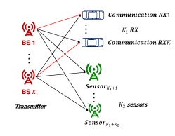
Figure 1: The ISAC Scenarios

However, sensing and communication operate on distinct information processing principles. To delve into the essence of the “integration” gain in ISAC systems, substantial research has been conducted on the information theoretic tradeoffs between communication and sensing performance based on these metrics. The information theoretic ISAC work was originally proposed in [6, 7] for the monostatic ISAC system with state-dependent discrete memoryless channels and i.i.d. state sequence to be estimated. The capacity-distortion region was characterized by a conditional mutual information maximized over some conditional probability satisfying some constraints. In order to explicitly characterize the close-form of the fundamental tradeoff between the communication and sensing performances, Xiong et al. considered the MIMO Gaussian channel in [8] and aimed to search the Cramer-Rao Bound (CRB)-rate region. Two extreme tradeoff points were characterized in [8], a.k.a, the communication-optimal point and the sensing-optimal point, which also reveal two fundamental aspects of tradeoffs in ISAC systems: subspace tradeoffs and deterministic-random tradeoffs. For the fixed sensing state where the state to be sensed remains fixed throughout one transmission block, the optimal tradeoff between the communication rate and state detection error exponent was characterized in [9]. Although research on communication-sensing tradeoffs has made some progress, it remains an open question[10, 11].

The aforementioned works mainly studied the monostatic ISAC systems, where the state is estimated by leveraging the communication message as the side information. Compared to monostatic sensing, bistatic sensing, by using separate sensor and transmitter, can avoid direct reflections or interference signals and cover larger areas, providing advantages in the detection of low-altitude and ground targets and also in the utilization of multipath signals for target detection [12]. Information theoretic ISAC works on the bistatic model basically focused on two cases, depending on the location of the communication receiver and sensor. For the bistatic ISAC model with co-located receiver and sensor, the capacity-distortion region for the i.i.d. state sequence was characterized in [13] and achievable region for the fixed state was proposed in [14].

For the bistatic ISAC model with dispersed receiver(s) and sensor, whose fundamental tradeoff between communication and sensing performances is generally open. A key challenge is that communication messages act as interference for the sensor. The authors in [15] introduced three achievable decoding-and-estimation strategies for the sensor which does not necessarily recover the communication message, i.e., blind estimation (e.g., the strategy of treating interference as noise as in [16]), partial-decoding-based estimation (e.g., the strategy of successive interference cancellation (SIC) as in [17]), and full-decoding-based estimation (i.e., first fully decoding the communication message and then estimating). Considering the general distortion function as the sensing metric, the achievable the rate-distortion regions by these three strategies in [15] are in the form of single-letter regions with auxiliary random variables.

Main Contributions

This paper considers the bistatic ISAC model with dispersed multi-receivers and one sensor. In order to characterize the fundamental tradeoff between the communication and sensing performances, we consider ‘homogeneous’ metrics, say communication degree of freedom (cDoF) and sensing degree of freedom (sDoF), which represent the average numbers of effective transmissions and observations in each time slot, respectively. As a new interference management strategy for perfectly eliminating the interference to the sensor in the bistatic ISAC model, we use the blind interference alignment (BIA) strategy in [18], with the assumption that the channel between the transmitters and the sensor is in slow-fading unknown to the transmitters and the channel between the transmitters and the communication receivers is in fast-fading known to the transmitters. This assumption is motivated by the following practical considerations: (i) Communication channels vary relatively quickly (with a coherence time of approximately 1-10 ms) because communication users are mobile. Furthermore, communication channels are periodically estimated via uplink/downlink (UL/DL) reciprocity and uplink pilots. Through these pilots, Channel State Information (CSI) at the transmitter is obtained. Here, for simplicity, we assume perfect CSI and do not consider pilot overhead or the actual channel estimation process. (ii) Sensing channels, in contrast, vary slowly since the sensors are stationary. Additionally, sensors and targets may be passive, meaning they do not transmit uplink pilots or provide channel state feedback. As a result, even though the channel varies slowly, this CSI remains unknown to the transmitter. We consider three types of wireless channels, including interference channels, multi-user MISO (MU-MISO) channels, and multi-user MIMO (MU-MIMO) channels. By using BIA, we propose new tradeoff points between cDoF and sDoF, which are strictly better than the time-sharing between the two extreme sensing-optimal and communication-optimal points. Finally, we take the simulation on the ISAC systems with QPSK modulation and additive white Gaussian noise. The proposed scheme improves the method by treating interference as noise at the sensor, with a gain of approximately [7, 75] dB.

Notation Convention

We adopt boldface letters to refer to vectors (lower case) and matrices (upper case). Sets are denoted using calligraphic symbols. Sans-serif symbols denote system parameters. For an arbitrary-size matrix ${\mathbf{M}}$, $\text{rank}({\mathbf{M}})$, ${\mathbf{M}}^{*}$, ${\mathbf{M}}^{T}$, and ${\mathbf{M}}^{H}$ represent its rank, conjugate, transpose, and conjugate transpose, respectively.$\lceil\cdot\rceil$ represents the ceiling function, which denotes rounding up to the nearest integer.The spaces of $x\times y$ complex and real matrices are denoted by $\mathbb{C}^{x\times y}$ and $\mathbb{R}^{x\times y}$, respectively.

II System Model

II-A Channel Model

Consider a bistatic ISAC system, where ${\mathsf{K}}_{T}$ ISAC transmitters are equipped with ${\mathsf{m}}_{i}$ antennas each $(i=1,2,\dots,{\mathsf{K}}_{T})$, and ${\mathsf{K}}_{R}$ communication receivers are equipped with ${\mathsf{n}}_{j}$ antennas each $(j=1,2,\dots,{\mathsf{K}}_{R})$. The sensor is equipped with single antenna. The channel outputs at the ${\mathsf{K}}_{R}$ communication receivers and at the sensor at the $t$-th time slot are as follows:

$${\mathbf{y}}_{c}^{[k]}(t)=\negmedspace\negmedspace\sum_{i=1}^{{\mathsf{K}}_{T}}\negmedspace{\mathbf{H}}_{c}^{[ki]}(t){\mathbf{x}}^{[i]}(t)+{\mathbf{z}}^{[k]}(t),\ k=\{1,\dots,{\mathsf{K}}_{R}\},$$ (1)

$$y_{s}(t)=\sum_{i=1}^{{\mathsf{K}}_{T}}{\mathbf{H}}_{s}^{[({\mathsf{K}}_{R}+1)i]}(t){\mathbf{x}}^{[i]}(t)+z_{s}(t),$$ (2)

where ${\mathbf{H}}_{c}^{[ki]}(t)\in\mathbb{C}^{{\mathsf{n}}_{k}\times{\mathsf{m}}_{i}}$ represents the channel from the $i$-th transmitter to the $k$-th communication user at time slot $t$, and ${\mathbf{H}}_{s}^{[({\mathsf{K}}_{R}+1)i]}(t)\in\mathbb{C}^{{\mathsf{n}}_{s}\times{\mathsf{m}}_{i}}$ represents the channel from the $i$-th transmitter to the sensor at time slot $t$. ${\mathbf{z}}^{[k]}(t)\in\mathbb{C}^{{\mathsf{n}}_{k}\times 1}$ and $z_{s}(t)\in\mathbb{C}$ are the additive Gaussian white noise at the receivers and sensor, respectively, with each element distributed as $\mathcal{CN}(0,1)$.

Assume that each transmission block spans $t_{0}$ channel uses. The signal transmitted by each transmitter $i\in\{1,2,\ldots,{\mathsf{K}}_{T}\}$ at time slot $t\in\{1,2,\ldots,t_{0}\}$ is the sum of a communication signal and a dedicated sensing signal:

$${\mathbf{x}}^{[i]}(t)={\mathbf{x}}_{c}^{[i]}(t)+{\mathbf{x}}_{s}^{[i]}(t).$$ (3)

The transmitted signal ${\mathbf{x}}^{[i]}(t)$ satisfies the power constraint $\mathbb{E}[|{\mathbf{x}}^{[i]}(t)|^{2}]\leq P$. ${\mathbf{x}}_{c}^{[i]}(t)\in\mathbb{C}^{{\mathsf{m}}_{i}}$ represents the communication signal, generated by the product of some precoding matrix and some vector of message symbols, and the dedicated sensing signal ${\mathbf{x}}_{s}^{[i]}(t)\in\mathbb{C}^{{\mathsf{m}}\times 1}$ is fixed and thus known to all the receivers and sensor.

In this paper, we assume that the communication channels follow a block fading model with a short coherence time and sensing channels follow a block fading model with a long coherence time. This is due to the mobility difference between receivers and the sensor, the communication channels are mobile, but have a short delay spread, while the sensing channels are more stationary, but have a large delay spread. It is true assuming that the sensors are looking at a vast environment with objects at much different relative distances. Changes in the sensed environment cause variations in the sensing channel, and these changes occur slowly relative to the coherence time of the communication channel. The channel varies for each transmission in every time slot, and we assume it follows Rayleigh fading, where both the real and imaginary parts of the channel coefficients are independent and identically distributed Gaussian variables with zero mean and variance of 1 (normal distribution).

By varying the number of antennas at the transmitter and receiver, we consider three different channel models:

• Interference Channel. When ${\mathsf{K}}_{T}={\mathsf{K}}_{R}={\mathsf{K}}$, ${\mathsf{m}}_{i}=1$ for each $i=1,2,\ldots,{\mathsf{K}}_{T}$, and ${\mathsf{n}}_{j}=1$ for each $j=1,2,\ldots,{\mathsf{K}}_{R}$, we obtain the interference channel as shown in Fig. 2(a). Note that in the interference channel, the message symbols requested by the $i$-th communication receiver are only known by the $i$-th transmitter.

• MU-MISO channel. When ${\mathsf{K}}_{T}=1$, ${\mathsf{K}}_{R}={\mathsf{K}}$, ${\mathsf{m}}_{1}={\mathsf{m}}$, and ${\mathsf{n}}_{j}=1$ for each $j=1,2,\ldots,{\mathsf{n}}$, we obtain the MU-MISO channel as shown in Fig. 2(a).

• MU-MIMO channel. When ${\mathsf{K}}_{T}=1,{\mathsf{K}}_{R}={\mathsf{K}},{\mathsf{m}}_{1}={\mathsf{m}}$, we obtain the MU-MIMO channel as shown in Fig. 2(c).

An additional assumption for the MU-MISO and MU-MIMO channels is that the channel states of two channels are causally known to the transmitters, meaning that the transmitter knows the channel states of the whole block in advance.

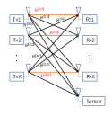
(a)

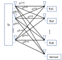
(b)

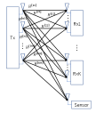
(c)

Figure 2: System Model. (a) Interference channel, (b) MU-MISO channel, (c) MU-MIMO channel.

II-B Performance Metrics

II-B1 Communication Degree of Freedom

For the performance metric of communications, we consider the sum-DoF per time slot averaged over $t_{0}$ time slots, denoted by CDoF. Recall that each message symbol carries one communication DoF; CDoF equals the total number of message symbols recovered by all communication receivers divided by $t_{0}$, for some $t_{0}$.

II-B2 Sensing Degree of Freedom

In order to facilitate characterizing the fundamental tradeoff between communications and sensing, we use ‘homogeneous’ metrics for them. Thus we consider the sensing degree of freedom based on the number of effective observations of the target during the estimation and detection process as in [19]. More precisely, assuming the total number of transmission antennas is ${\mathsf{m}}^{\prime}$, $N$ effective observations represents that the transmitter sends ${\mathbf{x}}_{1}^{[0]},{\mathbf{x}}_{2}^{[0]},\ldots,{\mathbf{x}}_{N}^{[0]}$ orthogonal sensing signals over $N$ different time slots, where

$$\begin{bmatrix}{\mathbf{x}}_{1}^{[0]},{\mathbf{x}}_{2}^{[0]},\ldots,{\mathbf{x}}_{N}^{[0]}\end{bmatrix}\begin{bmatrix}{\mathbf{x}}_{1}^{[0]},{\mathbf{x}}_{2}^{[0]},\ldots,{\mathbf{x}}_{N}^{[0]}\end{bmatrix}^{H}=I,$$ (4)

and the sensor obtains the receives signal over $N$ times. The sensing DoF, denoted by SDoF, is the total number of effective observations divided by $t_{0}$, for some $t_{0}$.

Objective: The objective of this paper is to characterize the capacity region of all achievable tradeoff points $(\text{SDoF},\text{CDoF})$.

III Main Results

The main contribution of this paper is to introduce the strategy of BIA into the bistatic ISAC systems to completely eliminate the interference from the communication messages at the sensor, under the constraint that the sensor channel is unknown to all. In addition, since the dedicated sensing signals are known to the communication receivers while decoding the desired messages, the communication receivers can first eliminate the sensing signals; to eliminate the interference from the undesired communication message for each communication receiver, the zero forcing scheme is used. In the following, we present the achievable regions by the proposed schemes for the three types of channels, respectively.

Theorem 1

For the bistatic ISAC systems with interference channel including ${\mathsf{K}}$ single-antenna transmitters, ${\mathsf{K}}$ single-antenna communication receivers, and one sensor, the lower convex envelop of the following tradeoff points are achievable

$$(\text{sDoF},\text{cDoF})=((K-1)/K,1);$$ (5)

and $(\text{sDoF},\text{cDoF})=(1,0)$, $(\text{sDoF},\text{cDoF})=(0,1)$, where the latter two points are achieved by the existing sensing-only scheme and communication-only scheme.

Theorem 2

For the bistatic ISAC systems with the MU-MISO channel including one transmitter with ${\mathsf{m}}$ antennas, ${\mathsf{K}}$ single-antenna communication receivers, and one sensor, the lower convex envelop of the following tradeoff points are achievable

$$(\text{sDoF},\text{cDoF})=\left(\frac{\left\lceil\frac{{\mathsf{m}}}{{\mathsf{K}}}\right\rceil-1}{\left\lceil\frac{{\mathsf{m}}}{{\mathsf{K}}}\right\rceil},\frac{{\mathsf{m}}}{\left\lceil\frac{{\mathsf{m}}}{{\mathsf{K}}}\right\rceil}\right);$$ (6)

and $(\text{sDoF},\text{cDoF})=(1,0)$, $(\text{sDoF},\text{cDoF})=(0,\min\{{\mathsf{m}},{\mathsf{K}}\})$, where the later two points are achieved by the existing sensing-only scheme and communication-only scheme.

Theorem 3

For the bistatic ISAC systems with the MU-MIMO channel including one transmitter with ${\mathsf{m}}$ antennas, ${\mathsf{K}}$ multi-antenna communication receivers (with the number of antennas ${\mathsf{n}}_{i},i=1,\ldots,{\mathsf{K}}$), and one sensor, the lower convex envelop of the following tradeoff points are achievable

$$(\text{sDoF},\text{cDoF})=\left(\frac{\left\lceil\frac{{\mathsf{m}}}{\sum_{k=1}^{{\mathsf{K}}}{\mathsf{n}}_{k}}\right\rceil-1}{\left\lceil\frac{{\mathsf{m}}}{\sum_{k=1}^{{\mathsf{K}}}{\mathsf{n}}_{k}}\right\rceil},\frac{{\mathsf{m}}}{\left\lceil\frac{{\mathsf{m}}}{\sum_{k=1}^{{\mathsf{K}}}{\mathsf{n}}_{k}}\right\rceil}\right);$$ (7)

and $(\text{sDoF},\text{cDoF})=(1,0)$, $(\text{sDoF},\text{cDoF})=(0,\min\{{\mathsf{m}},\sum_{k=1}^{{\mathsf{K}}}{\mathsf{n}}_{k}\})$, where the later two points are achieved by the existing sensing-only scheme and communication-only scheme.

The detailed proofs of Theorems 1-3 could be found in the extended version of this paper [20].

IV Achievable Schemes

In this section, we describe the main ideas of the proposed schemes based on the BIA strategy through two examples for the interference channel and MU-MISO channel, respectively.

IV-A Example 1: Interference Channel

Consider the bistatic ISAC system with interference channel including $3$ single-antenna transmitters, $3$ single-antenna communication receivers, and one sensor, as illustrated in Fig. 3. For this system, the tradeoff points $(\text{sDoF},\text{cDoF})=(1,0)$, $(\text{sDoF},\text{cDoF})=(0,1)$ can be achieved by the sensing-only scheme and communication-only scheme, respectively. We then propose an ISAC scheme combining BIA and zero-forcing, achieving $(\text{sDoF},\text{cDoF})=(2/3,1)$.

Let $t_{0}=3$. Let the communication signals in the $3$ time slots by each transmitter $k\in\{1,2,3\}$ be $\textbf{x}^{[k]}_{c}(1)=\textbf{x}^{[k]}_{c}(2)=\textbf{x}^{[k]}_{c}(3)=W^{[k]}$, where $W^{[k]}\in{\mathbb{C}}$ represents a message symbol desired by the $k$-th communication receiver. Thus by removing the dedicated sensing signals (which are deterministic), at time $t$ for the $k$-th communication receiver obtains:

$$\hat{{\mathbf{y}}}^{[k]}=\begin{bmatrix}\hat{Y}^{[k]}(1)\\ \hat{Y}^{[k]}(2)\\ \hat{Y}^{[k]}(3)\end{bmatrix} =\sum_{i=1}^{3}\begin{bmatrix}H^{[ki]}(1)\textbf{x}^{[k]}_{c}(1)\\ H^{[ki]}(2)\textbf{x}^{[k]}_{c}(2)\\ H^{[ki]}(3)\textbf{x}^{[k]}_{c}(3)\end{bmatrix}+\begin{bmatrix}{\mathbf{z}}^{[k]}(1)\\ {\mathbf{z}}^{[k]}(2)\\ {\mathbf{z}}^{[k]}(3)\end{bmatrix}$$

$$=\sum_{i=1}^{3}\begin{bmatrix}H^{[ki]}(1)\\ H^{[ki]}(2)\\ H^{[ki]}(3)\end{bmatrix}W^{[i]}+\begin{bmatrix}{\mathbf{z}}^{[k]}(1)\\ {\mathbf{z}}^{[k]}(2)\\ {\mathbf{z}}^{[k]}(3)\end{bmatrix}.$$ (8)

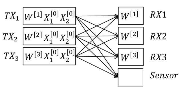
Figure 3: Example 1: Interference Channel

For the $k$-th communication receiver, we can apply the zero-forcing decoding to decode $W^{[}k]$ from $\hat{{\mathbf{y}}}^{[k]}$. Consequently, the achieved communication DoF is $3/3=1$.

The sensing DoF (SDoF) is $2/3$, meaning that $2$ effective observations can be obtained over $3$ time slots. Next, we demonstrate the signal design using blind interference alignment. Let ${\mathbf{x}}_{1}^{[0]}=[x_{1,1},x_{1,2},x_{1,3}]^{T}\in{\mathbb{C}}^{3\times 1}$ and ${\mathbf{x}}_{2}^{[0]}=[x_{2,1},x_{2,2},x_{2,3}]^{T}\in{\mathbb{C}}^{3\times 1}$, satisfying $[{\mathbf{x}}_{1}^{[0]},{\mathbf{x}}_{2}^{[0]}][{\mathbf{x}}_{1}^{[0]},{\mathbf{x}}_{2}^{[0]}]^{H}=I$. Our idea is to use the fact that the channel for the sensor remains constant over a certain period and that the communication signals also remain constant to cancel the communication signals, which are interference for the sensor. For the $k$-th transmitter where $k\in\{1,2,3\}$, the transmitted signals over $3$ time slots are: $\textbf{x}^{[k]}(1)=W^{[i]}+x_{1,i}+x_{2,i}$, $\textbf{x}^{[k]}(2)=W^{[k]}+x_{2,i}$, $\textbf{x}^{[k]}(3)=W^{[i]}+x_{1,i}$. The signals received by the sensor can be expressed as:

$${\mathbf{y}}^{[4]}_{s}=\begin{bmatrix}y^{[4]}_{s}(1)\\ y^{[4]}_{s}(2)\\ y^{[4]}_{s}(3)\end{bmatrix}$$

$$=\sum_{i=1}^{3}\begin{bmatrix}H^{[4i]}(1)(W^{[i]}+x_{1,i}+x_{2,i})\\ H^{[4i]}(1)(W^{[i]}+x_{2,i})\\ H^{[4i]}(1)(W^{[i]}+x_{1,i})\end{bmatrix}+\begin{bmatrix}z_{s}(1)\\ z_{s}(2)\\ z_{s}(3)\end{bmatrix}.$$

By subtracting the observations at the second and third time slots from the first time slot, we get:

$${\mathbf{y}}_{s}^{[4]}(1)-{\mathbf{y}}_{s}^{[4]}(t) =\sum_{i=1}^{3}H^{[4i]}(1)x_{t-1,i}+z_{s}(1)-z_{s}(t)$$

$$={\mathbf{h}}\begin{bmatrix}x_{t-1,1}\\ x_{t-1,2}\\ x_{t-1,3}\end{bmatrix}+z_{s}(1)-z_{s}(t),$$

where ${\mathbf{h}}=\begin{bmatrix}H^{[41]}(1),H^{[42]}(1),H^{[43]}(1)\end{bmatrix}$ and $t={2,3}$. Therefore, the sensor obtains ${\mathbf{h}}{\mathbf{x}}_{1}^{[0]}+z_{s}(1)-z_{s}(2)$ and ${\mathbf{h}}{\mathbf{x}}_{2}^{[0]}+z_{s}(1)-z_{s}(3)$, meaning two effective observations over three time slots. Thus the SDoF is $2/3$, and the achieved tradeoff point by the proposed scheme is $(\text{sDoF},\text{cDoF})=(2/3,1)$. Considering the three achieved tradeoff points, the lower convex envelope is plotted by the blue line in Fig. 5(a), while the red line represents the time-sharing between the sensing-only and communication-only points. It can be seen that the achieved point by the proposed scheme significantly improves the one by time-sharing.

IV-B Example 2: MU-MISO Channel

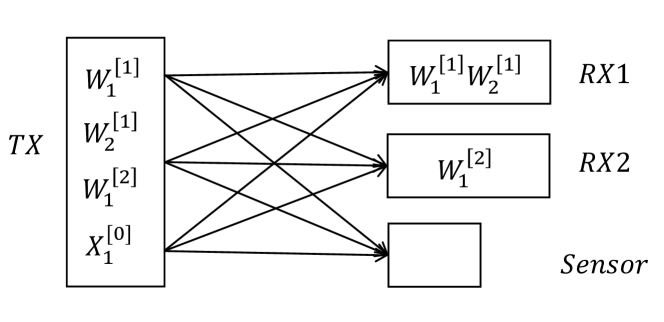
Figure 4: Example 2: MU-MISO channel

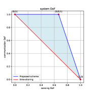
(a)

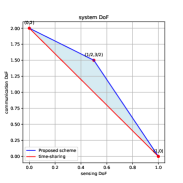
(b)

Figure 5: Sensing DoF v.s. Communication DoF. (a) Interference channels, (b) MU-MISO channels.

We then consider the bistatic ISAC systems with the MU-MISO channel including one transmitter with $3$ antennas, $2$ single-antenna communication receivers, and one sensor, as illustrated in Fig. 4. For this system, the tradeoff points $(\text{sDoF},\text{cDoF})=(1,0)$, $(\text{sDoF},\text{cDoF})=(0,2)$ can be achieved by the sensing-only scheme and communication-only scheme, respectively.

Let $t_{0}=2$. Over the two slots, the first communication receiver decodes two symbols $W_{1}^{[1]}$ and $W_{2}^{[1]}$; the second communication receiver decodes one symbol $W_{1}^{[2]}$. Let the communication signals transmitted at time slot $t\in\{1,2\}$ be

$${\mathbf{x}}_{c}(t)={\mathbf{v}}_{1}^{[1]}W_{1}^{[1]}+{\mathbf{v}}_{2}^{[1]}W_{2}^{[1]}+{\mathbf{v}}_{1}^{[2]}W_{1}^{[2]},$$

where ${\mathbf{v}}_{j}^{[i]}\in{\mathbb{C}}^{3\times 1}$ is the precoding vector for $W_{j}^{[i]}$. By removing the dedicated sensing signals, the $k$-th communication receiver obtains at time slot $t$:

$$\hat{{\mathbf{y}}}^{[k]}(t) =\begin{bmatrix}H^{[k1]}(t)&H^{[k2]}(t)&H^{[k3]}(t)\end{bmatrix}{\mathbf{x}}_{c}(t)+{\mathbf{z}}^{[k]}(t).$$

The precoding vectors are designed such that, (i) the first communication receiver decodes $W_{1}^{[1]}$ from $\hat{{\mathbf{y}}}^{[1]}(1)$ and decodes $W_{2}^{[1]}$ from $\hat{{\mathbf{y}}}^{[1]}(2)$, (ii) the second communication receiver decodes $W_{1}^{[2]}$ from $\hat{{\mathbf{y}}}^{[1]}(1)$. Hence, let ${\mathbf{v}}_{1}^{[1]}$ be a null vector of the matrix:

$$\begin{bmatrix}H^{[21]}(1)&H^{[22]}(1)&H^{[23]}(1)\\ H^{[11]}(2)&H^{[12]}(2)&H^{[13]}(2)\end{bmatrix};$$

let ${\mathbf{v}}_{2}^{[1]}$ be a null vector of the matrix:

$$\begin{bmatrix}H^{[21]}(1)&H^{[22]}(1)&H^{[23]}(1)\\ H^{[11]}(1)&H^{[12]}(1)&H^{[13]}(1)\end{bmatrix};$$

and let ${\mathbf{v}}_{1}^{[2]}$ be a null vector of the matrix:

$$\begin{bmatrix}H^{[11]}(1)&H^{[12]}(1)&H^{[13]}(1)\\ H^{[11]}(2)&H^{[12]}(2)&H^{[13]}(2)\end{bmatrix}.$$

As a result, over 2 time slots, $3$ symbols are totally decoded; thus the achieved communication DoF is $3/2$.

Similar to the previous example, since the communication signals remain constant across 2 time slots, we can obtain one effective observation for sensing, ${\mathbf{x}}_{1}^{[0]}\in{\mathbb{R}}^{3\times 1}=[x_{1,1},x_{1,2},x_{1,3}]^{T}$. Let the transmitted signals over two time slots are: $\textbf{x}^{[k]}(1)={\mathbf{x}}_{c}(1)+{\mathbf{x}}_{1}^{[0]}$, $\textbf{x}^{[k]}(2)={\mathbf{x}}_{c}(2)$, for each $k\in\{1,2\}$. The messages received by the sensor can be expressed as:

$${\mathbf{y}}^{[3]}_{s}=\begin{bmatrix}y^{[3]}_{s}(1)\\ y^{[3]}_{s}(2)\end{bmatrix}=\begin{bmatrix}{\mathbf{h}}^{[3]}(1)({\mathbf{x}}_{c}(1)+{\mathbf{x}}_{1}^{[0]})\\ {\mathbf{h}}^{[3]}(1){\mathbf{x}}_{c}(2)\end{bmatrix}+\begin{bmatrix}z_{s}(1)\\ z_{s}(2)\end{bmatrix}.$$ (9)

By subtracting the observations at the second time slot from the first time slot, we get:

$$\begin{aligned} {\mathbf{y}}_{s}^{[3]}(1)-{\mathbf{y}}_{s}^{[3]}(2)={\mathbf{h}}^{[3]}(1){\mathbf{x}}_{1}^{[0]}+z_{s}(1)-z_{s}(2),\end{aligned},$$ (10)

where ${\mathbf{h}}^{[3]}(1)=\begin{bmatrix}H^{[31]}(1),H^{[32]}(1),H^{[33]}(1)\end{bmatrix}$. Therefore, the sensor obtains ${\mathbf{h}}^{[3]}(1){\mathbf{x}}_{1}^{[0]}+z_{s}(1)-z_{s}(2)$, meaning one effective observation over $2$ time slots. Thus the SDoF is $1/2$, and the achieved tradeoff point is $(\text{sDoF},\text{cDoF})=(1/2,3/2)$. Considering the three achieved tradeoff points, the lower convex envelope is plotted by the blue line in Fig. 5(b). It can be seen that the achieved point by the proposed scheme significantly improves the one by time-sharing.

V Simulation Results

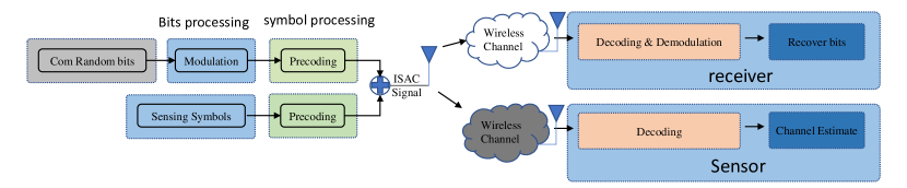
Figure 6: Simulation flowchart

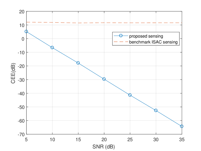
Figure 7: simulation result

In this section, we simulate the interference channel example in Section IV-A (with $3$ single-antenna transmitters, $3$ single-antenna communication receivers, and one sensor) and compare it with the method by treating interference as noise at the sensor. The simulation setting is as follows: the communication symbols are modulated by QPSK modulation. The distance between the transmitter and the communication receiver is between $[50,100]$ meters, and the distance between the transmitter and the sensor is between $[10,30]$ meters. The fixed transmission power for both the communication signal and the sensing signal is set to $30$ dBm, and the channel fading characteristics follow a Rayleigh distribution, with the SNR set to $[5,35]$ dB. As in Section IV-A, the transmitters have perfect CSI of communication channels but lack prior information about the sensing channel, and the dedicated sensing signal is a deterministic signal known by both the transmitting and receiving ends. The simulation flowchart is shown in Fig. 6.

For the sensing task, we use the LS estimation method to estimate the channel, given by $\hat{{\mathbf{H}}}=({\mathbf{X}}^{\mathbf{H}}{\mathbf{X}})^{-1}{\mathbf{X}}^{\mathbf{H}}{\mathbf{Y}}$, where $\hat{{\mathbf{H}}}$ represents the estimated channel, ${\mathbf{X}}$ represents the sensing signal, and ${\mathbf{Y}}$ represents the received signal. Since the LS method is very sensitive to noise, we observe the performance differences under SNR values ranging from [5, 35] dB. Analysis shows that at higher SNR conditions, the proposed method is less affected, and the channel estimation error (CEE) decreases with increasing SNR. The CEE is defined as $\text{CEE}=\|{\mathbf{H}}-\hat{{\mathbf{H}}}\|^{2}$, where ${\mathbf{H}}$ is the actual channel state, $\hat{{\mathbf{H}}}$ is the estimate channel state, $\|\cdot\|$ denotes the norm of the vector, commonly the Euclidean norm. In contrast, the reference method treats the communication signal as noise, so even with low noise power, the high transmission power of the communication signal results in poor estimation accuracy, with minimal changes in CEE as SNR increases. In comparison, our method provides a gain of [7, 75] dB in estimation accuracy, while the communication performances (i.e., communication rate or bit error rate) of the two methods are the same.

Appendix A Proof of Theorem 3

In this appendix, we will further expand upon the previous example to make it more general. At first, we will demonstrate how the system achieves

$$(\text{SDoF},\text{CDoF})=\left(\frac{{\mathsf{K}}-1}{{\mathsf{K}}},1\right),$$ (11)

in the case of a ${\mathsf{K}}\times{\mathsf{K}}$ interference channel with an additional sensor. First, let’s analyze the receivers. The signal received by the $k\in{1,2,\dots,{\mathsf{K}}}$-th receiver is:

$${\mathbf{y}}^{[k]}(t)=H^{[k1]}(t)({\mathbf{x}}_{c}^{[1]}(t)+{\mathbf{x}}_{s}^{[1]}(t))+H^{[k2]}(t)({\mathbf{x}}_{c}^{[2]}(t)\\ +{\mathbf{x}}_{s}^{[2]}(t))+\dots+H^{[k{\mathsf{K}}]}(t)({\mathbf{x}}_{c}^{[{\mathsf{K}}]}(t)+{\mathbf{x}}_{s}^{[{\mathsf{K}}]}(t))+{\mathbf{z}}^{[k]}(t)$$ (12)

Similarly, since the CSI and the transmitted sensing signal ${\mathbf{x}}_{s}^{[k]}(t)$ are known to the communication users, we can cancel this part of the signal at the receiver, resulting in an estimate $\hat{{\mathbf{y}}}^{[k]}$ that only concerns the communication signals:

$$\hat{{\mathbf{y}}}^{[k]}(t)=H^{[k1]}(t){\mathbf{x}}_{c}^{[1]}(t)+H^{[k2]}(t){\mathbf{x}}_{c}^{[2]}(t)+\dots+\\ H^{[k{\mathsf{K}}]}(t){\mathbf{x}}^{[{\mathsf{K}}]}(t)+{\mathbf{z}}^{[k]}(t)$$ (13)

Using the same method as in the previous section, we combine the channel matrices experienced by all the undesired signals to obtain ${\mathbf{H}}_{\text{cob}}$, and it is easy to find that $\text{rank}({\mathbf{H}}_{\text{cob}})={\mathsf{K}}-1$. The dimension of its row space is ${\mathsf{K}}$, so the dimension of its left null space should be ${\mathsf{K}}-({\mathsf{K}}-1)=1$. Let this vector be ${\mathbf{v}}_{k}\in\mathbb{C}^{1\times{\mathsf{K}}}$, and following the same steps as before, we can obtain ${\mathbf{x}}_{c}^{[k]}(t)$. Thus, we achieve a total of ${\mathsf{K}}$ degrees of freedom over ${\mathsf{K}}$ time slots, and the communication degrees of freedom (CDoF) of the system is ${\mathsf{K}}/{\mathsf{K}}=1$.

For the sensor, we can obtain ${\mathsf{K}}-1$ sensing signals over ${\mathsf{K}}$ time slots, with ${\mathbf{x}}_{k}^{[0]}for(k=1,2,\dots,{\mathsf{K}}-1)$. The transmitted sensing signals need to satisfy our constraint $[{\mathbf{x}}_{1}^{[0]},{\mathbf{x}}_{2}^{[0]},\dots,{\mathbf{x}}_{{\mathsf{K}}-1}^{[0]}][{\mathbf{x}}_{1}^{[0]},{\mathbf{x}}_{2}^{[0]},\dots,{\mathbf{x}}_{{\mathsf{K}}-1}^{[0]}]^{H}=I$. Besides transmitting the fixed signal ${\mathbf{x}}^{[k]}(t)$ at each time slot, the $k$-th transmitter also needs to transmit the sensing signal, which we present in matrix form. In our previous toy example, the transmitted signal was already given by the equation, and we can see that the encoding for the transmitted sensing signal is the same; we only need to ensure that after subtracting the signals at two different time slots, the corresponding coefficient’s parameter is 1, as follows:

$$\begin{bmatrix}x_{(1,k)}+x_{(2,k)}\\ x_{(2,k)}\\ x_{(1,k)}\end{bmatrix}=\begin{bmatrix}1&1\\ 0&1\\ 1&0\end{bmatrix}\begin{bmatrix}x_{(1,k)}\\ x_{(2,k)}\end{bmatrix}$$ (14)

The encoding matrix for the sensing signal to be transmitted is not full-rank. From the perspective of solving the equation, any encoding method can be used to solve for the desired sensing signal, as long as the encoding matrix’s columns are full-rank. However, since the actual sensing system does not know the encoding method used by the transmitter, we must ensure that the desired signal can be obtained by the simplest operation at the receiver. We can write out the encoding method for ${\mathsf{K}}$ users:

$$\begin{bmatrix}x_{(1,k)}+x_{(2,k)}+x_{(3,k)}+\dots+x_{({\mathsf{K}}-1,k)}\\ x_{(2,k)}+x_{(3,k)}+\dots+x_{({\mathsf{K}}-1,k)}\\ x_{(1,k)}+x_{(3,k)}+\dots+x_{({\mathsf{K}}-1,k)}\\ \vdots\\ x_{(1,k)}+x_{(2,k)}+\dots+x_{({\mathsf{K}}-2,k)}\end{bmatrix}$$ (15)

$$=\begin{bmatrix}1&1&1&\dots&1\\ 0&1&1&\dots&1\\ 1&0&1&\dots&1\\ \vdots&\vdots&\vdots&\ddots&\vdots\\ 1&1&1&\dots&0\end{bmatrix}\begin{bmatrix}x_{(1,k)}\\ x_{(2,k)}\\ x_{(3,k)}\\ \vdots\\ x_{({\mathsf{K}}-1,k)}\end{bmatrix}$$

In this encoding scheme, since the interference channel requires transmitting the same signal over ${\mathsf{K}}$ time slots to decode the corresponding communication signal, we only need to subtract the received values at other time slots from the received value at the first time slot to obtain the result at time $t$:

$${\mathbf{y}}_{s}^{[{\mathsf{K}}+1]}(1)-{\mathbf{y}}_{s}^{[{\mathsf{K}}+1]}(t)=H^{[{\mathsf{K}}+1,1]}(1)x_{(t-1,1)}+\\ H^{[{\mathsf{K}}+1,2]}(1)x_{(t-1,2)}+\dots+H^{[{\mathsf{K}}+1,{\mathsf{K}}]}(1)x_{(t-1,{\mathsf{K}})}+{\mathbf{z}}_{s}(1)-{\mathbf{z}}_{s}(t)$$ (16)

In matrix multiplication form:

$$\begin{bmatrix}H^{[{\mathsf{K}}+1,1]}(1),H^{[{\mathsf{K}}+1,2]}(1),\dots,H^{[{\mathsf{K}}+1,{\mathsf{K}}]}(1)\end{bmatrix}\begin{bmatrix}x_{(t-1,1)}\\ x_{(t-1,2)}\\ x_{(t-1,3)}\\ \vdots\\ x_{(t-1,{\mathsf{K}})}\end{bmatrix}$$ (17)

Thus, at each time slot after the first, we can obtain an effective observation of the channel. Over ${\mathsf{K}}$ time slots, we obtain ${\mathsf{K}}-1$ effective observations, and the sensing degrees of freedom (SDoF) is $\frac{{\mathsf{K}}-1}{{\mathsf{K}}}$.

Appendix B Proof of Theorem 4

We consider a common system with a transmitter equipped with ${\mathsf{m}}$ antennas, ${\mathsf{n}}$ single-antenna receivers, and a sensor with a single antenna. We denote the channel matrix from the transmitter to the receiver at time $t$ as:

$${\mathbf{H}}(t)=\begin{bmatrix}H^{[11]}(t)&H^{[12]}(t)&\ldots&H^{[1{\mathsf{m}}]}(t)\\ H^{[21]}(t)&H^{[22]}(t)&\ldots&H^{[2{\mathsf{m}}]}(t)\\ \vdots&\vdots&\ddots&\vdots\\ H^{[{\mathsf{n}}1]}(t)&H^{[{\mathsf{n}}2]}(t)&\ldots&H^{[{\mathsf{n}}{\mathsf{m}}]}(t)\end{bmatrix},$$ (18)

where $H^{[ij]}(t)$ represents the channel from the $j$-th transmit antenna to the $i$-th receive antenna at time $t$. To obtain the demand $W_{t}^{[i]}$ for receiver $i$, we demonstrate the pre-coding matrix obtained using the zero forcing method. The matrix ${\mathbf{H}}_{unexp}^{i}(t)$, composed of all non-expected channel elements at non-expected times for receiver $i$, is given by:

$${\mathbf{H}}_{unexp}^{i}(t)=\begin{bmatrix}{\mathbf{H}}(1)\\ {\mathbf{H}}(2)\\ \vdots\\ {\mathbf{H}}(t)\backslash{\mathbf{H}}(t)[i,:]\\ \vdots\\ {\mathbf{H}}\left(\left\lceil\frac{{\mathsf{m}}}{{\mathsf{n}}}\right\rceil\right)\end{bmatrix},$$ (19)

where ${\mathbf{H}}(t)[i,:]$ denotes the $i$-th row of ${\mathbf{H}}(t)$, and ${\mathbf{H}}(t)/{\mathbf{H}}(t)[i,:]$ represents the matrix ${\mathbf{H}}(t)$ with the $i$-th row removed, $\lceil{\mathsf{m}}/{\mathsf{n}}\rceil$ denotes the ceiling of ${\mathsf{m}}/{\mathsf{n}}$. ${\mathbf{H}}(\lceil{\mathsf{m}}/{\mathsf{n}}\rceil)$ is given by:

$$\begin{bmatrix}H^{[11]}\left(\left\lceil\frac{{\mathsf{m}}}{{\mathsf{n}}}\right\rceil\right)&H^{[12]}\left(\left\lceil\frac{{\mathsf{m}}}{{\mathsf{n}}}\right\rceil\right)&\cdots&H^{[1{\mathsf{m}}]}\left(\left\lceil\frac{{\mathsf{m}}}{{\mathsf{n}}}\right\rceil\right)\\ H^{[21]}\left(\left\lceil\frac{{\mathsf{m}}}{{\mathsf{n}}}\right\rceil\right)&H^{[22]}\left(\left\lceil\frac{{\mathsf{m}}}{{\mathsf{n}}}\right\rceil\right)&\cdots&H^{[2{\mathsf{m}}]}\left(\left\lceil\frac{{\mathsf{m}}}{{\mathsf{n}}}\right\rceil\right)\\ \vdots&\vdots&\ddots&\vdots\\ H^{[p1]}\left(\left\lceil\frac{{\mathsf{m}}}{{\mathsf{n}}}\right\rceil\right)&H^{[p2]}\left(\left\lceil\frac{{\mathsf{m}}}{{\mathsf{n}}}\right\rceil\right)&\cdots&H^{[p{\mathsf{m}}]}\left(\left\lceil\frac{{\mathsf{m}}}{{\mathsf{n}}}\right\rceil\right)\end{bmatrix},$$ (20)

where $p={\mathsf{m}}\mod{\mathsf{n}}$. By analyzing the dimensions of the matrix, we know that the null space of ${\mathbf{H}}_{\text{unexp}}^{i}(t)$ is non-empty. Therefore, we can use the vector ${\mathbf{v}}^{[i]}(t)$ in its null space to encode the transmitted signal such that it is nulled out for other recievers or at undesired time slots. So we can get the ISAC signal :

$${\mathbf{x}}(t)=({\mathbf{v}}^{[1]}(1)W_{1}^{[1]}+{\mathbf{x}}_{s}^{[1]}(t))+\dots+({\mathbf{v}}^{[{\mathsf{n}}]}({\left\lceil\frac{{\mathsf{m}}}{{\mathsf{n}}}\right\rceil})W_{\left\lceil\frac{{\mathsf{m}}}{{\mathsf{n}}}\right\rceil}^{[{\mathsf{n}}]}+{\mathbf{x}}_{s}^{[{\mathsf{n}}]}(t))$$ (21)

In this way, we can continuously transmit the coded communication signal over $\left\lceil\frac{{\mathsf{m}}}{{\mathsf{n}}}\right\rceil$ time slots, and the communication signals decoded at each time slot are different, ensuring the communication degrees of freedom (DoF) in the system. On this basis, blind interference alignment can also be utilized to achieve higher sensing degrees of freedom. For receiver $i$, the received signal at time $t$ is given by:

$$\hat{{\mathbf{y}}}^{[i]}(t) =\begin{bmatrix}H^{[i1]}(t)&H^{[i2]}(t)&\dots&H^{[i{\mathsf{m}}]}(t)\end{bmatrix}{\mathbf{x}}(t)+{\mathbf{z}}^{[i]}(t)$$

$$=\begin{bmatrix}H^{[i1]}(t)&H^{[i2]}(t)&\dots&H^{[i{\mathsf{m}}]}(t)\end{bmatrix}{\mathbf{v}}^{[i]}(t)W_{t}^{[i]}$$

$$+{\mathbf{z}}^{[i]}(t)$$

$$={\mathbf{H}}(t)[i,:]{\mathbf{v}}^{[i]}(t)W_{t}^{[i]}+{\mathbf{z}}^{[i]}(t),$$ (22)

where all the non-user $i$ signals or signals not required at time $t$ are pre-coded by ${\mathbf{v}}^{[j]}(\tau)$ (where $\tau=t$ and $i=j$ cannot hold simultaneously) , which is a vector in the null space of the experienced channel matrix ${\mathbf{H}}(t)[i,:]$ . Therefore, after multiplying, these signals become zero. Based on the channel polynomial and the received signal, we can decode $W_{t}^{[i]}$. With ${\mathsf{n}}$ single-antenna users, we can achieve ${\mathsf{n}}$ communication degrees of freedom at $\left\lceil\frac{{\mathsf{m}}}{{\mathsf{n}}}\right\rceil$ time slots. For the sensor:

$${\mathbf{y}}_{s}^{[{\mathsf{n}}+1]}(t)={\mathbf{h}}^{[{\mathsf{n}}+1]}(t){\mathbf{x}}(t)+z_{s}(t),$$ (23)

where ${\mathbf{h}}^{[{\mathsf{n}}+1]}(t)=\begin{bmatrix}H^{[{\mathsf{n}}+1,1]}(t)&\dots&H^{[{\mathsf{n}}+1,{\mathsf{m}}]}(t)\end{bmatrix}$. Similar to the previous analysis, since the communication signal remains constant over $\left\lceil\frac{{\mathsf{m}}}{{\mathsf{n}}}\right\rceil$ time slots, we can obtain $\left\lceil\frac{{\mathsf{m}}}{{\mathsf{n}}}\right\rceil-1$ effective observations of ${\mathbf{x}}_{1}^{[0]},{\mathbf{x}}_{2}^{[0]},\dots,{\mathbf{x}}_{\left\lceil\frac{{\mathsf{m}}}{{\mathsf{n}}}\right\rceil-1}^{[0]}$. And they satisfy the orthogonality condition we require. Let ${\mathbf{x}}_{j}^{[0]}=\begin{bmatrix}x_{(j,1)},x_{(j,2)},x_{(j,3)},\dots,x_{(j,{\mathsf{m}})}\end{bmatrix}$, and we can obtain the sensing signal to be transmitted by the $k$-th antenna at the transmitter as:

$$\begin{bmatrix}x_{(1,k)}+x_{(2,k)}+x_{(3,k)}+\dots+x_{(\left\lceil\frac{{\mathsf{m}}}{{\mathsf{n}}}\right\rceil-1,k)}\\ x_{(2,k)}+x_{(3,k)}+\dots+x_{(\left\lceil\frac{{\mathsf{m}}}{{\mathsf{n}}}\right\rceil-1,k)}\\ x_{(1,k)}+x_{(3,k)}+\dots+x_{(\left\lceil\frac{{\mathsf{m}}}{{\mathsf{n}}}\right\rceil-1,k)}\\ \vdots\\ x_{(1,k)}+x_{(2,k)}+\dots+x_{(\left\lceil\frac{{\mathsf{m}}}{{\mathsf{n}}}\right\rceil-2,k)}\end{bmatrix}$$ (24)

$$=\begin{bmatrix}1&1&1&\dots&1\\ 0&1&1&\dots&1\\ 1&0&1&\dots&1\\ \vdots&\vdots&\vdots&\ddots&\vdots\\ 1&1&1&\dots&0\end{bmatrix}\begin{bmatrix}x_{(1,k)}\\ x_{(2,k)}\\ x_{(3,k)}\\ \vdots\\ x_{(\left\lceil\frac{{\mathsf{m}}}{{\mathsf{n}}}\right\rceil-1,k)}\end{bmatrix}.$$

Thus, Since the sensor experiences a slow fading process, the channel remains constant over several time slots, and the communication signal remains constant as well. The sensor can subtract the received signal at time slot $t$ from the received signal at the first time slot:

$${\mathbf{y}}_{s}^{[{\mathsf{n}}+1]}(1)-{\mathbf{y}}_{s}^{[{\mathsf{n}}+1]}(t) ={\mathbf{h}}^{[{\mathsf{n}}+1]}(1){\mathbf{x}}(1)-{\mathbf{h}}^{[{\mathsf{n}}+1]}(t){\mathbf{x}}(t)$$

$$+{\mathbf{z}}_{s}(1)-{\mathbf{z}}_{s}(t)$$

$$={\mathbf{h}}^{[{\mathsf{n}}+1]}(t){\mathbf{x}}(1)-{\mathbf{h}}^{[{\mathsf{n}}+1]}(t){\mathbf{x}}(t)$$

$$+{\mathbf{z}}_{s}(1)-{\mathbf{z}}_{s}(t)$$

$$={\mathbf{h}}^{[{\mathsf{n}}+1]}(t)({\mathbf{x}}^{[0]}(1)-{\mathbf{x}}^{[0]}(t))$$

$$+{\mathbf{z}}_{s}(1)-{\mathbf{z}}_{s}(t)$$

$$={\mathbf{h}}^{[{\mathsf{n}}+1]}(t){\mathbf{x}}_{t-1}^{[0]}+{\mathbf{z}}_{s}(1)-{\mathbf{z}}_{s}(t),$$ (25)

thereby canceling the interference caused by the communication signals and obtaining an effective observation of ${\mathbf{x}}_{t-1}^{[0]}$. Over $\left\lceil\frac{{\mathsf{m}}}{{\mathsf{n}}}\right\rceil$ time slots, a total of $\left\lceil\frac{{\mathsf{m}}}{{\mathsf{n}}}\right\rceil-1$ effective observations can be made, and the sensing degrees of freedom (SDoF) is $\left\lceil\frac{{\mathsf{m}}}{{\mathsf{n}}}\right\rceil-1/\left\lceil\frac{{\mathsf{m}}}{{\mathsf{n}}}\right\rceil$.

The system’s total sensing and communication degrees of freedom are $(\text{SDoF},\text{CDoF})=\left(\frac{\left\lceil\frac{{\mathsf{m}}}{{\mathsf{n}}}\right\rceil-1}{\left\lceil\frac{{\mathsf{m}}}{{\mathsf{n}}}\right\rceil},{\mathsf{n}}\right)$. For an ${\mathsf{m}}\times{\mathsf{n}}$ system, we only need to ensure that the number of antennas at the transmitter is an integer multiple of the number of antennas at the receiver. In this way, we can achieve sensing and communication degrees of freedom $\left(\frac{\left\lceil\frac{{\mathsf{m}}}{{\mathsf{n}}}\right\rceil-1}{\left\lceil\frac{{\mathsf{m}}}{{\mathsf{n}}}\right\rceil},{\mathsf{n}}\right)$. Although increasing the number of antennas generally increases the communication degrees of freedom in the system, due to the limitation on the number of antennas at the receiver, the maximum number of linearly independent data streams that can be transmitted at one time is restricted. Thus, the originally available degrees of freedom can be repurposed as sensing degrees of freedom.

Appendix C Proof of Theorem 5

To generalize the model, we further extend it to the case where the number of antennas at the receiver can be arbitrary. We consider a more common system with a transmitter equipped with ${\mathsf{m}}$ antennas, ${\mathsf{K}}$ receivers, and a sensor with a single antenna, we modify the number of antennas at the $k$-th receiver to ${\mathsf{n}}_{k}$($k=1,2,\ldots{\mathsf{K}}$). The channel matrix from the transmitter to the $k$-th receiver at time $t$ is denoted as $\mathbf{H}^{[k]}(t)\in\mathbb{C}^{{\mathsf{n}}_{k}\times{\mathsf{m}}}$.

$${\mathbf{H}}^{[k]}(t)=\begin{bmatrix}H^{[11]}(t)&H^{[12]}(t)&\cdots&H^{[1{\mathsf{m}}]}(t)\\ H^{[21]}(t)&H^{[22]}(t)&\cdots&H^{[2{\mathsf{m}}]}(t)\\ \vdots&\vdots&\ddots&\vdots\\ H^{[{\mathsf{n}}_{k}1]}(t)&H^{[{\mathsf{n}}_{k}2]}(t)&\cdots&H^{[{\mathsf{n}}_{k}{\mathsf{m}}]}(t)\end{bmatrix},$$ (26)

where $H^{[ji]}(t)$ denotes the channel coefficient from the $i$-th antenna of the transmitter to the $j$-th antenna of user $k$. Similar to previous discussions, we first consider the communication task in isolation. At time $t$, the signal that reciever $k$ expects to receive is denoted as $W_{i}^{[k]}(t)$ (where $i=1,2,\ldots,{\mathsf{n}}_{k}$). Using the same approach, we aim to encode the signal such that it is zeroed out at non-desired targets and non-desired times.

For user $k$, the matrix of non-desired times and targets that the signal $W_{i}^{[k]}(t)$ experiences at time $t$ can be represented as:

$${\mathbf{H}}_{(t-\text{unexp})}^{[k]}=\begin{bmatrix}{\mathbf{H}}^{[1]}(1)\\ \vdots\\ {\mathbf{H}}^{[1]}(\left\lceil\frac{{\mathsf{m}}}{\sum_{k=1}^{{\mathsf{K}}}{\mathsf{n}}_{k}}\right\rceil)\\ \vdots\\ {\mathbf{H}}^{[k]}(1)\\ \vdots\\ {\mathbf{H}}^{[k]}(t-1)\\ {\mathbf{H}}^{[k]}(t+1)\\ \vdots\\ {\mathbf{H}}^{[k]}\left(\left\lceil\frac{{\mathsf{m}}}{\sum_{k=1}^{{\mathsf{K}}}{\mathsf{n}}_{k}}\right\rceil\right)\end{bmatrix}.$$ (27)

$${\mathbf{H}}^{[k]}(\left\lceil\frac{{\mathsf{m}}}{\sum_{k=1}^{{\mathsf{K}}}{\mathsf{n}}_{k}}\right\rceil)=\begin{cases}\begin{bmatrix}H^{[11]}\left(\frac{{\mathsf{m}}}{\sum_{k=1}^{{\mathsf{K}}}{\mathsf{n}}_{k}}\right)&H^{[12]}\left(\frac{{\mathsf{m}}}{\sum_{k=1}^{{\mathsf{K}}}{\mathsf{n}}_{k}}\right)&\cdots&H^{[1{\mathsf{m}}]}\left(\frac{{\mathsf{m}}}{\sum_{k=1}^{{\mathsf{K}}}{\mathsf{n}}_{k}}\right)\\ H^{[21]}\left(\frac{{\mathsf{m}}}{\sum_{k=1}^{{\mathsf{K}}}{\mathsf{n}}_{k}}\right)&H^{[22]}\left(\frac{{\mathsf{m}}}{\sum_{k=1}^{{\mathsf{K}}}{\mathsf{n}}_{k}}\right)&\cdots&H^{[2{\mathsf{m}}]}\left(\frac{{\mathsf{m}}}{\sum_{k=1}^{{\mathsf{K}}}{\mathsf{n}}_{k}}\right)\\ \vdots&\vdots&\ddots&\vdots\\ H^{[{\mathsf{n}}_{k}1]}\left(\frac{{\mathsf{m}}}{\sum_{k=1}^{{\mathsf{K}}}{\mathsf{n}}_{k}}\right)&H^{[{\mathsf{n}}_{k}2]}\left(\frac{{\mathsf{m}}}{\sum_{k=1}^{{\mathsf{K}}}{\mathsf{n}}_{k}}\right)&\cdots&H^{[{\mathsf{n}}_{k}{\mathsf{m}}]}\left(\frac{{\mathsf{m}}}{\sum_{k=1}^{{\mathsf{K}}}{\mathsf{n}}_{k}}\right)\end{bmatrix},&\sum_{i=1}^{k}{\mathsf{n}}_{i}<p\\ \begin{bmatrix}H^{[11]}\left(\frac{{\mathsf{m}}}{\sum_{k=1}^{{\mathsf{K}}}{\mathsf{n}}_{k}}\right)&H^{[12]}\left(\frac{{\mathsf{m}}}{\sum_{k=1}^{{\mathsf{K}}}{\mathsf{n}}_{k}}\right)&\cdots&H^{[1{\mathsf{m}}]}\left(\frac{{\mathsf{m}}}{\sum_{k=1}^{{\mathsf{K}}}{\mathsf{n}}_{k}}\right)\\ H^{[21]}\left(\frac{{\mathsf{m}}}{\sum_{k=1}^{{\mathsf{K}}}{\mathsf{n}}_{k}}\right)&H^{[22]}\left(\frac{{\mathsf{m}}}{\sum_{k=1}^{{\mathsf{K}}}{\mathsf{n}}_{k}}\right)&\cdots&H^{[2{\mathsf{m}}]}\left(\frac{{\mathsf{m}}}{\sum_{k=1}^{{\mathsf{K}}}{\mathsf{n}}_{k}}\right)\\ \vdots&\vdots&\ddots&\vdots\\ H^{[q1]}\left(\frac{{\mathsf{m}}}{\sum_{k=1}^{{\mathsf{K}}}{\mathsf{n}}_{k}}\right)&H^{[q2]}\left(\frac{{\mathsf{m}}}{\sum_{k=1}^{{\mathsf{K}}}{\mathsf{n}}_{k}}\right)&\cdots&H^{[q{\mathsf{m}}]}\left(\frac{{\mathsf{m}}}{\sum_{k=1}^{{\mathsf{K}}}{\mathsf{n}}_{k}}\right)\end{bmatrix},&p<\sum_{i=1}^{k}{\mathsf{n}}_{i}<p+{\mathsf{n}}_{k}\\ \emptyset,&\text{else}\end{cases}$$ (28)

where in equation (28) $p={\mathsf{m}}\mod\sum_{k=1}^{{\mathsf{K}}}{\mathsf{n}}_{k}$, let the last $k$ satisfying the first condition be $k_{1}$, and $q=p-\sum_{i=1}^{k_{1}}n_{i}$. To better understand, we take an example where the transmitter has 6 antennas, the receiver has two communication users each with two antennas, and one sensing user with a single antenna. We hope the first communication user (CU1) can decode 4 symbols in two time slots, and the second communication user (CU2) can decode 2 symbols in two time slots. Similar to the previous section, the undesired matrix for CU1 at the first time slot can be written as:

$${\mathbf{H}}_{(1-\text{unexp})}^{[1]}=\begin{bmatrix}{\mathbf{H}}^{[1]}(2)\\ {\mathbf{H}}^{[2]}(1)\end{bmatrix}.$$ (29)

We can see that this matrix is a $4\times 6$ matrix. Therefore, we can use its null space to find two zero vectors ${\mathbf{v}}_{1}^{[1]}(1)$ and ${\mathbf{v}}_{2}^{[1]}(1)$ to encode the symbols to be transmitted. Similarly, we can obtain the encoding vectors for the other two symbols. Finally, we get the transmitted communication signal:

$${\mathbf{x}}_{c}(t)=\sum_{t=1}^{2}\sum_{i=1}^{2}{\mathbf{v}}_{i}^{[1]}(t)W_{i}^{[1]}(t)+\sum_{j=1}^{2}{\mathbf{v}}_{j}^{[2]}(1)W_{j}^{[2]}(1).$$ (30)

Thus, except for the channel experienced by user $k$ at time $t$, all other channels are zeroed out. In this way, the receiver can decode the desired signal. Therefore, we can decode the received signal using the channel parameters polynomial and the pre-coding matrix. The communication degrees of freedom obtained in 2 time slots are $6/2=3$. For the sensor, the received signal is:

$${\mathbf{y}}_{s}^{[3]}(t)={\mathbf{h}}^{[3]}(t)({\mathbf{x}}_{c}(t)+{\mathbf{x}}_{s}(t))+{\mathbf{z}}_{s}(t).$$ (31)

Similar to the analysis of the MISO system, since the communication signal remains unchanged in 2 time slots, we can use the signal ${\mathbf{x}}_{1}^{[0]}$ to obtain effective observations of the target. Let ${\mathbf{x}}_{1}^{[0]}\in\mathbb{C}^{6\times 1}$, satisfying our orthogonality requirements. Let ${\mathbf{x}}_{1}^{[0]}=[x_{1,1},x_{1,2},x_{1,3},\ldots,x_{1,{\mathsf{m}}}]^{T}$, then the transmitted signal is:

$$\begin{bmatrix}{\mathbf{x}}_{s}(1)\\ {\mathbf{x}}_{s}(2)\end{bmatrix}=\begin{bmatrix}{\mathbf{x}}_{1}^{[0]}\\ 0\end{bmatrix}.$$ (32)

In this way, the sensing user only needs to subtract the received signal at the 2nd time slot from the received signal at the 1st time slot to eliminate the interference caused by the communication signal.

$${\mathbf{y}}_{s}^{[3]}(1)-{\mathbf{y}}_{s}^{[3]}(2)={\mathbf{h}}^{[3]}(1){\mathbf{x}}_{1}^{[0]}+{\mathbf{z}}_{s}(1)-{\mathbf{z}}_{s}(2).$$ (33)

Therefore, we obtain ${\mathbf{h}}^{[3]}(1){\mathbf{x}}_{1}^{[0]}$ , meaning one effective observations over three time slots. Thus, the SDoF is 1/2, and the overall system degrees of freedom for sensing and communication are (SDoF, CDoF) = (1/2, 3).

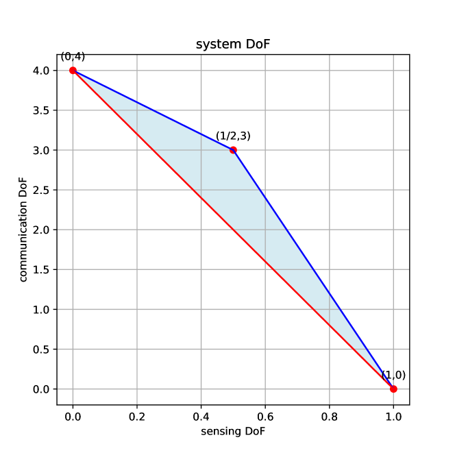
Figure 8: system DoF vs timesharing DoF

By decomposing this system, if we only have the 6×4 communication MU-MIMO channel, we can see that the degrees of freedom for sensing and communication are (SDoF, CDoF) = (0, 4). If there is only one sensing user, the degrees of freedom are (SDoF, CDoF) = (1, 0).By the time-sharing method, we can plot the trade-off curve of degrees of freedom obtained by combining two discrete systems, as shown by the red line in the figure. Furthermore, using our proposed method, a new inflection point (SDoF, CDoF) = (1/2, 3) can be obtained, resulting in a new curve, as illustrated by the blue line in the figure 8.

The following argument is intended to generalize the proofs provided earlier and also unveils the fundamental principle behind our zero-forcing and blind interference alignment scheme. For the transmitter, we set the number of transmit antennas to be greater than the number of receiver antennas for each user. In this setup, the transmitter has extra degrees of freedom that can be leveraged to design a zero-forcing precoding matrix, enabling the implementation of blind interference alignment. Essentially, this approach embodies a trade-off between communication and sensing capabilities.

For the initial $\left\lceil\frac{{\mathsf{m}}}{\sum_{k=1}^{{\mathsf{K}}}{\mathsf{n}}_{k}}\right\rceil$ time slots $t$ ($t=1,2,\dots,\left\lceil\frac{{\mathsf{m}}}{\sum_{k=1}^{{\mathsf{K}}}{\mathsf{n}}_{k}}\right\rceil-1$), we assume that $\left\lceil\frac{{\mathsf{m}}}{\sum_{k=1}^{{{\mathsf{K}}}}{\mathsf{n}}_{k}}\right\rceil\geq 1$. This assumption does not compromise the generality of the result since, for values less than $1$, certain receiver antennas would not be fully utilized. During this period, all antennas at each receiver are fully utilized, allowing each user $k$ to achieve ${\mathsf{n}}_{k}$ degrees of freedom. For each user $k$, it suffices to ensure that, at time $t$, the desired signals $W_{i}^{[k]}(t)$ $(i=1,2,\dots,{\mathsf{n}}_{k})$ are aligned by zero-forcing precoding vectors ${\mathbf{v}}_{i}^{[k]}(t)$, such that other users and other times are zero-forced. Thus, we can express the resulting signals as $\sum_{i=1}^{{\mathsf{n}}_{k}}H^{[k]}(t){\mathbf{v}}_{i}^{[k]}(t)W_{i}^{[k]}(t)$, and obtain the following matrix:

$$\begin{bmatrix}H^{[k]}(t){\mathbf{v}}_{1}^{[k]}(t)&H^{[k]}(t){\mathbf{v}}_{2}^{[k]}(t)&\dots&H^{[k]}(t){\mathbf{v}}_{n_{k}}^{[k]}(t)\end{bmatrix}$$ (34)

This matrix has dimensions ${\mathsf{m}}\times n_{k}$, and we can select vectors from its null space to decode the desired signals $W_{i}^{[k]}(t)$. When $t=\left\lceil\frac{{\mathsf{m}}}{\sum_{k=1}^{{{\mathsf{K}}}}n_{k}}\right\rceil$, it is evident that not all users’ antennas will be utilized at this time. However, we focus on antennas that are in use, without further elaboration. For users falling under the second case in the formula, the number of symbols transmitted to them is $q$. Likewise, we can use zero-forcing precoding to encode these $q$ symbols. By this point, we fully utilize the “extra” degrees of freedom provided by the multiple antennas at the transmitter, and ensure that the communication symbols remain constant over $\left\lceil\frac{{\mathsf{m}}}{\sum_{k=1}^{{{\mathsf{K}}}}n_{k}}\right\rceil$ time slots to increase the degrees of freedom for sensing, so we can get ${\mathsf{m}}$ cDoF in $\left\lceil\frac{{\mathsf{m}}}{\sum_{k=1}^{{{\mathsf{K}}}}n_{k}}\right\rceil$ time slots, system cDoF is $\frac{{\mathsf{m}}}{\left\lceil\frac{{\mathsf{m}}}{\sum_{k=1}^{{{\mathsf{K}}}}n_{k}}\right\rceil}$.

At the sensor, we acquire $\left\lceil\frac{{\mathsf{m}}}{\sum_{k=1}^{{{\mathsf{K}}}}n_{k}}\right\rceil-1$ effective observations within $\left\lceil\frac{{\mathsf{m}}}{\sum_{k=1}^{{{\mathsf{K}}}}n_{k}}\right\rceil$ time slots, where one time slot is used to cancel the effects of communication signals at the receiver, and each other time slot yields a new effective observation, so system sDoF is $\frac{\left\lceil\frac{{\mathsf{m}}}{\sum_{k=1}^{{{\mathsf{K}}}}n_{k}}\right\rceil-1}{\left\lceil\frac{{\mathsf{m}}}{\sum_{k=1}^{{{\mathsf{K}}}}n_{k}}\right\rceil}$.

References

- [1] W. Saad, M. Bennis, and M. Chen, “A vision of 6g wireless systems: Applications, trends, technologies, and open research problems,” IEEE network, vol. 34, no. 3, pp. 134–142, 2019.
- [2] D. K. P. Tan, J. He, Y. Li, A. Bayesteh, Y. Chen, P. Zhu, and W. Tong, “Integrated sensing and communication in 6g: Motivations, use cases, requirements, challenges and future directions,” in 2021 1st IEEE International Online Symposium on Joint Communications & Sensing (JC&S). IEEE, 2021, pp. 1–6.
- [3] F. Liu, Y. Cui, C. Masouros, J. Xu, T. X. Han, Y. C. Eldar, and S. Buzzi, “Integrated sensing and communications: Toward dual-functional wireless networks for 6g and beyond,” IEEE journal on selected areas in communications, vol. 40, no. 6, pp. 1728–1767, 2022.
- [4] F. Liu, C. Masouros, A. Li, H. Sun, and L. Hanzo, “Mu-mimo communications with mimo radar: From co-existence to joint transmission,” IEEE Transactions on Wireless Communications, vol. 17, no. 4, pp. 2755–2770, 2018.
- [5] F. Liu, C. Masouros, A. P. Petropulu, H. Griffiths, and L. Hanzo, “Joint radar and communication design: Applications, state-of-the-art, and the road ahead,” IEEE Transactions on Communications, vol. 68, no. 6, pp. 3834–3862, 2020.
- [6] M. Kobayashi, G. Caire, and G. Kramer, “Joint state sensing and communication: Optimal tradeoff for a memoryless case,” in 2018 IEEE International Symposium on Information Theory (ISIT), 2018, pp. 111–115.
- [7] M. Ahmadipour, M. Kobayashi, M. Wigger, and G. Caire, “An information-theoretic approach to joint sensing and communication,” IEEE Transactions on Information Theory, vol. 70, no. 2, pp. 1124–1146, 2022.
- [8] Y. Xiong, F. Liu, Y. Cui, W. Yuan, T. X. Han, and G. Caire, “On the fundamental tradeoff of integrated sensing and communications under gaussian channels,” IEEE Transactions on Information Theory, vol. 69, no. 9, pp. 5723–5751, 2023.
- [9] H. Joudeh and F. M. Willems, “Joint communication and binary state detection,” IEEE Journal on Selected Areas in Information Theory, vol. 3, no. 1, pp. 113–124, 2022.
- [10] A. Liu, Z. Huang, M. Li, Y. Wan, W. Li, T. X. Han, C. Liu, R. Du, D. K. P. Tan, J. Lu et al., “A survey on fundamental limits of integrated sensing and communication,” IEEE Communications Surveys & Tutorials, vol. 24, no. 2, pp. 994–1034, 2022.
- [11] Y. Xiong, F. Liu, K. Wan, W. Yuan, Y. Cui, and G. Caire, “From torch to projector: Fundamental tradeoff of integrated sensing and communications,” IEEE BITS the Information Theory Magazine, pp. 1–13, 2024.
- [12] N. J. Willis and H. D. Griffiths, Advances in bistatic radar. SciTech Publishing, 2007, vol. 2.
- [13] W. Zhang, S. Vedantam, and U. Mitra, “Joint transmission and state estimation: A constrained channel coding approach,” IEEE Transactions on Information Theory, vol. 57, no. 10, pp. 7084–7095, 2011.
- [14] M.-C. Chang, S.-Y. Wang, T. Erdoğan, and M. R. Bloch, “Rate and detection-error exponent tradeoff for joint communication and sensing of fixed channel states,” IEEE Journal on Selected Areas in Information Theory, vol. 4, pp. 245–259, 2023.
- [15] T. Jiao, Y. Geng, Z. Wei, K. Wan, Z. Yang, and G. Caire, “Information-theoretic limits of bistatic integrated sensing and communication,” arXiv e-prints, pp. arXiv–2306, 2023.
- [16] Y. Dong, F. Liu, and Y. Xiong, “Joint receiver design for integrated sensing and communications,” IEEE Communications Letters, vol. 27, no. 7, pp. 1854–1858, 2023.
- [17] C. Ouyang, Y. Liu, and H. Yang, “Revealing the impact of sic in noma-isac,” IEEE Wireless Communications Letters, vol. 12, no. 10, pp. 1707–1711, 2023.
- [18] S. A. Jafar, “Blind interference alignment,” IEEE Journal of Selected Topics in Signal Processing, vol. 6, no. 3, pp. 216–227, 2012.
- [19] L. Xie, F. Liu, J. Luo, and S. Song, “Sensing mutual information with random signals in gaussian channels: Bridging sensing and communication metrics,” arXiv preprint arXiv:2402.03919, 2024.
- [20] J. Liu, K. Wan, X. Yi, R. C. Qiu, and G. Caire, “Interference alignment scheme for integrated sensing and communications,” 2024, gitHub repository. [Online]. Available: https://github.com/saneyu/Interference-alignment-scheme-for-integrated-sensing-and-communications
- [21] H. Liu and E. Alsusa, “A novel isac approach for uplink noma system,” IEEE Communications Letters, 2023.