CO-to-H₂ conversion factor and grain size distribution through the analysis of $\alpha_{\mathrm{CO}}$–$q_{\mathrm{PAH}}$ relation

Abstract

The CO-to-H₂ conversion factor ($\alpha_{\mathrm{CO}}$) is expected to vary with dust abundance and grain size distribution through the efficiency of shielding gas from CO-dissociation radiation. We present a comprehensive analysis of $\alpha_{\mathrm{CO}}$ and grain size distribution for nearby galaxies, using the PAH fraction ($q_{\mathrm{PAH}}$) as an observable proxy of grain size distribution. We adopt the resolved observations at 2 kpc resolution in 42 nearby galaxies, where $\alpha_{\mathrm{CO}}$ is derived from measured metallicity and surface densities of dust and H i assuming a fixed dust-to-metals ratio. We use an analytical model for the evolution of H₂ and CO, in which the evolution of grain size distribution is controlled by the dense gas fraction ($\eta$). We find that the observed level of $q_{\mathrm{PAH}}$ is consistent with the diffuse-gas-dominated model ($\eta=0.2$) where dust shattering is more efficient. Meanwhile, the slight decreasing trend of observed $q_{\mathrm{PAH}}$ with metallicity is more consistent with high-$\eta$ predictions, likely due to the more efficient loss of PAHs by coagulation. We discuss how grain size distribution (indicated by $q_{\mathrm{PAH}}$) and metallicity impact $\alpha_{\mathrm{CO}}$; we however did not obtain conclusive evidence that the grain size distribution affects $\alpha_{\mathrm{CO}}$. Observations and model predictions show similar anti-correlation between $\alpha_{\mathrm{CO}}$ and 12+log(O/H). Meanwhile, there is a considerable difference in how resolved $\alpha_{\mathrm{CO}}$ behaves with $q_{\mathrm{PAH}}$. The observed $\alpha_{\mathrm{CO}}$ has a positive correlation with $q_{\mathrm{PAH}}$, while the model-predicted $\alpha_{\mathrm{CO}}$ does not have a definite correlation with $q_{\mathrm{PAH}}$. This difference is likely due to the limitation of one-zone treatment in the model.

1 Introduction

Stars form in cold, dense molecular clouds in the interstellar medium (ISM). Molecular gas fuels star formation, and is a key factor diagnosing star-forming conditions. Therefore, observing molecular gas is essential for understanding star formation and galaxy evolution. However, the major component of molecular gas, H₂, does not possess a permanent dipole moment and thus does not emit efficiently in cold molecular clouds. As a result, observers often use the low-$J$ ($J$ is the rotational energy level) emission lines of the second most abundant molecule, CO, to trace the molecular gas.

The standard practice for astronomers is to convert the observed CO $(1{\scalebox{0.75}[1.0]{$-$}}0)$ integrated intensity at wavelength $\lambda=1.3$ mm ($W_{\mathrm{CO}}$ [K km s^-1]) to molecular gas surface density ($\Sigma_{\mathrm{mol}}$ [M_☉ pc^-2]) or H₂ column density ($N\mathrm{(H_{2})}$ [cm^-2]) as follows:

$$\Sigma_{\mathrm{mol}}=\alpha_{\rm CO}W_{\mathrm{CO}},~\mathrm{or}~N\mathrm{(H_{2})}=X_{\mathrm{CO}}W_{\mathrm{CO}},$$ (1)

where $\alpha_{\rm CO}$ and $X_{\mathrm{CO}}$ are the “CO-to-H₂ conversion factor” under different conventions. The conventional CO-to-H₂ conversion factor applicable to the Milky Way (MW) environment is $\alpha_{\rm CO}=4.35~{\rm M_{\odot}\,pc^{-2}\,(K\,km\,s^{-1})^{-1}}$ (see Bolatto et al., 2013), which corresponds to $X_{\mathrm{CO}}=2\times 10^{20}~\mathrm{cm^{-2}~(K~km~s^{-1})^{-1}}$. In this paper, we follow the $\alpha_{\rm CO}$ (or $\Sigma_{\mathrm{mol}}$) convention.

The CO-to-H₂ conversion factor is environment-dependent. Obtaining appropriate values of $\alpha_{\rm CO}$ for various environments is crucial to accurately constrain the initial conditions for star formation. Astronomers have found two major trends that set the value of $\alpha_{\rm CO}$. First, $\alpha_{\rm CO}$ tends to drop in galaxy centres, star-forming regions and (ultra-)luminous infrared (IR) galaxies (Downes et al., 1993; Downes & Solomon, 1998; Israel, 2009a, b, 2020; Weiß et al., 2001; Papadopoulos et al., 2012; Sandstrom et al., 2013; Herrero-Illana et al., 2019; Jiao et al., 2021; Teng et al., 2022, 2023; den Brok et al., 2023; Chiang et al., 2024). This is interpreted as $\alpha_{\rm CO}$ decreasing with the rise of the CO emissivity, which increases with gas density, temperature and optical depth. Secondly, $\alpha_{\rm CO}$ rises at low metallicity and low dust-to-gas ratio (D/G) environments. This is due to decreased shielding of CO-dissociating radiation and thus decreased CO-emitting area in molecular clouds, which is often phrased as ‘CO-dark’ gas (Arimoto et al., 1996; Israel, 1997; Papadopoulos et al., 2002; Grenier et al., 2005; Wolfire et al., 2010; Leroy et al., 2011; Planck Collaboration et al., 2011; Hunt et al., 2015; Accurso et al., 2017; Madden et al., 2020). Some of the latest observation-based formulae tracing the above mechanisms are summarized in the Schinnerer & Leroy (2024) review (see also Bolatto et al., 2013).

It is expected that the second effect—increased $\alpha_{\rm CO}$ at low metallicity—has a direct link to galaxy evolution through metal enrichment. The CO-dark gas is tightly linked to shielding of CO-dissociating radiation by gas and dust (e.g. Lee et al., 1996; Glover & Mac Low, 2011). Given the local physical conditions, $\alpha_{\rm CO}$ can in principle be derived theoretically by calculating the formation and destruction of H₂ and CO (e.g. Narayanan et al., 2011; Glover & Mac Low, 2011; Feldmann et al., 2012). Most existing formulae use a single parameter, i.e. metallicity or D/G, to trace the dust shielding. Recent modelling further investigated the effect of dust properties, especially focusing on the grain size distribution (Hirashita & Harada, 2017; Hirashita, 2023b, hereafter H23). These models show that even if the dust abundance is the same, different grain size distributions predict different shielding efficiencies of ultraviolet (UV) dissociating radiation as it changes the crosssections.

Based on the analytic approach of representing the grain size distribution at two grain radii by Hirashita & Harada (2017), Chen et al. (2018) post-processed a disc-galaxy simulation, and found that the difference in grain size distribution causes an appreciable change of the CO abundance. A grain size distribution with a higher portion of small grains tends to result in a higher CO abundance since smaller grains absorb UV radiation more efficiently at fixed dust abundance. This conclusion was confirmed with a full treatment of grain size distribution (without approximating it by two sizes) by H23, who showed that the evolution of grain size distribution regulated by the dense-gas fraction causes nearly an order-of-magnitude difference in $\alpha_{\rm CO}$ at sub-solar to solar metallicities. Therefore, the effect of grain size distribution should be quantitatively checked along with the interpretation of the metallicity dependence of $\alpha_{\rm CO}$.

In this paper, we examine the effect of grain size distribution on $\alpha_{\rm CO}$ using observations. Given that $\alpha_{\rm CO}$ is affected by the local physical conditions, we adopt the latest spatially resolved measurements of nearby galaxies by Chiang et al. (2024, hereafter C24). C24 compiled and analyzed multi-wavelength data for dust properties, neutral gas emission lines, and auxiliary information from $\sim 40$ nearby galaxies. They derived $\alpha_{\rm CO}$ from the surface densities of dust and H i and metallicity, assuming a constant dust-to-metals ratio (D/M). This results in $\sim 1400$ independent measurements of $\alpha_{\rm CO}$ across various environments in nearby star-forming galaxies at a uniform physical resolution of 2 kpc. This dataset provides a testing ground for understanding how $\alpha_{\rm CO}$ evolves with local physical conditions, especially dust properties.

An observational proxy for the grain size distribution is necessary for the above goal. Specifically, it is possible to extract information on the grain size distribution from the widely available IR data, e.g. from Herschel Space Observatory (Herschel, Pilbratt et al., 2010) far-IR and Wide-field Infrared Survey Explorer (WISE, Wright et al., 2010) mid-IR data. Since the C24 sample has abundant IR data, it also represents an ideal sample to extract information on the grain size distribution from the dust emission spectral energy distributions (SEDs). Polycyclic aromatic hydrocarbons (PAHs) are particularly useful as an observational tracer of small grains, since they have prominent features at mid-IR wavelengths. Meanwhile, the total dust abundance can be evaluated by analyzing the far-IR SED, allowing the fraction of PAH to total dust mass ($q_{\mathrm{PAH}}$) to be measured and then used as an observational proxy for the fraction of small grains, which in turn has a direct link to the grain size distribution. Indeed, Matsumoto et al. (2024) used $q_{\mathrm{PAH}}$ as an indicator of grain size distribution in their simulations and showed that the model-predicted $q_{\mathrm{PAH}}$ has a direct correspondence with the observed mid-IR PAH emission luminosity divided by the far-IR thermal emission. Therefore, $q_{\mathrm{PAH}}$ can potentially bridge the models and observations by acting as an indicator of grain size distribution.

In C24, $q_{\mathrm{PAH}}$ is one of the quantities obtained by fitting the Draine & Li (2007) physical dust model to the WISE mid-IR and Herschel far-IR photometry data. The fitting is performed in Chastenet et al. (2024), following the same methodology reported in Chastenet et al. (2021), and this is the same IR SED fitting used to estimate the dust surface density and so $\alpha_{\rm CO}$. This means that $q_{\mathrm{PAH}}$ is immediately available as an indicator of grain size distribution for all C24 targets and we use these $q_{\mathrm{PAH}}$ estimates as the default tracer for grain size distribution in the analysis. We also examine the $q_{\mathrm{PAH}}$ predicted by Hirashita (2023a), based on a model designed to reproduce the MW $q_{\mathrm{PAH}}$ and grain size distribution at solar metallicity.

This paper is organized as follows. In Section 2, we review the C24 observations, including the explanations of how $\alpha_{\rm CO}$ and dust properties are measured and derived. In Section 3, we give an overview of the H23 model. In Section 4, we present the observed relations among $q_{\mathrm{PAH}}$, $\alpha_{\rm CO}$ and metallicity, and how these trends compare to the model prediction. In Section 5, we discuss the interpretation of our results and other possible tracers for grain size distribution. Finally, we summarize our findings in Section 6.

2 Data

In this work, we utilize the spatially resolved measurements of $\alpha_{\rm CO}$ and other relevant physical quantities presented in C24. Here, we briefly describe the dataset and refer the reader to C24 for more details.

C24 assembled multi-wavelength data relevant for estimating the surface densities of various components, i.e. dust, neutral gas, stellar mass, SFR, and metallicity, in nearby galaxies. We compile data from 42 galaxies in our analysis, including the 37 presented in C24 and 5 additional ones. All the data are convolved to 2 kpc physical resolution ($\geq 21\arcsec$ angular resolution, depending on the distance) with pixel sizes of 2/3 kpc. We list the properties of all galaxies and references of adopted data in Appendix A. All galaxies have distances within $20\,\mathrm{Mpc}$ such that the lowest resolution data (dust or H i with $\sim 21\arcsec$ resolution) can be analyzed at a uniform 2 kpc resolution. The target galaxies are selected to have spatially resolved observation of neutral gas emission lines (H i 21 cm and either CO $(1{\scalebox{0.75}[1.0]{$-$}}0)$ at 115 GHz or CO $(2{\scalebox{0.75}[1.0]{$-$}}1)$ at 230 GHz) and maps from the $z$0MGS-Herschel/Dust catalogue (Chastenet et al., 2024). The $z$0MGS catalogue also includes auxiliary data in the mid-IR and UV, which trace surface densities of star formation rate (SFR) and stellar mass (denoted as $\Sigma_{\mathrm{SFR}}$ and $\Sigma_{\star}$, respectively; Leroy et al. 2019). To the best of our knowledge, this is the largest spatially resolved dataset with $\alpha_{\rm CO}$, $q_{\mathrm{PAH}}$, and metallicity. Below we briefly describe the quantities used in this paper and clarify some differences from C24.

CO-to-H₂ conversion factor. C24 measured $\alpha_{\rm CO}$ using a dust-based strategy. The key assumption in their method is a fixed value for the fraction of metals locked in the solid phase, i.e. D/M. They calculated the molecular gas surface density ($\Sigma_{\mathrm{mol}}$) from the measured values of dust surface density ($\Sigma_{\mathrm{dust}}$), atomic gas surface density (from H i), and metallicity under the assumed D/M. Then they divided the calculated $\Sigma_{\mathrm{mol}}$ by integrated CO intensity ($I_{\mathrm{CO}}$) to evaluate $\alpha_{\rm CO}$. The value of D/M adopted by C24 is 0.55; however, we adopt the value of 0.48 from H23 as the fiducial case in this work for consistency with the model (more details in Section 3). This change in D/M causes $\alpha_{\rm CO}$ to increase about 0.07 to 0.10 dex from the C24 values. We note that there are other strategies for converting dust observations to hydrogen mass, e.g. using a constant D/G (e.g. Boulanger et al., 1996), minimizing the scatter in D/G (e.g. Sandstrom et al., 2013), or nonlinear dust optical depth to $\Sigma_{\mathrm{gas}}$ conversion (e.g. Okamoto et al., 2017; Hayashi et al., 2019). We refer the readers to Bolatto et al. (2013) and C24 for the discussion of these methodologies.

Dust properties. The dust properties from the $z$0MGS-Herschel/Dust catalogue are derived by fitting the observed dust emission SED with the Draine & Li (2007) dust model. The details of the IR data processing and dust SED fitting are reported in Chastenet et al. (2024). The IR SED used in the fitting includes the WISE 3.4, 4.6, 12, and 22 µm bands, and the Hershel 70, 100, 160, and 250 µm bands. These IR maps are first convolved to circular Gaussian point spread functions at the final physical resolution (2 kpc) before the fitting. The dust SEDs are fitted using the Draine & Li (2007) physical dust model with dust opacity correction factor derived in Chastenet et al. (2021), applied through the DustBFF tool, which considers the full covariance matrix between photometry bands (Gordon et al., 2014). The product of fitting includes maps of the dust mass surface density ($\Sigma_{\mathrm{dust}}$), the interstellar radiation field (ISRF) properties ($U_{\mathrm{min}}$, $\gamma$ and $\overline{U}$), and the fractional mass of PAHs to total dust (PAH fraction, $q_{\mathrm{PAH}}$). We define the PAHs as small aromatic grains with radii $a<13$ Å (corresponding to $N_{C}\leq 10^{3}$ C atoms. see Equation 3 and Section 10.3 of Draine & Li, 2007) in both the SED fitting and the model calculations.

A specific caveat of using the Chastenet et al. (2024) dust properties in this study is that the grain size distribution is not explicitly fitted to the observations. Instead, they fit $q_{\mathrm{PAH}}$ and the grain size distribution almost solely varies with the inferred PAH abundance. This is different from the H23 model, where $q_{\mathrm{PAH}}$ is not the only factor that determines the functional form of grain size distribution. Practically, we expect that $q_{\mathrm{PAH}}$ and other dust properties derived from the SED fitting are not sensitive to the detailed assumptions regarding the grain size distribution. The evaluation of the total dust mass is dominated by the far-IR part of the SED, which is robust against the change of the grain size distribution, while the evaluation of the PAH mass is based on the level of the prominent PAH features. Therefore, $q_{\mathrm{PAH}}$ is practically determined by the PAH emission strength relative to the FIR luminosity, which is not affected by the detailed functional shape of the grain size distribution.

Metallicity. C24 used oxygen abundance, $12+\log({\rm O/H})$, to trace the metallicity ($Z$). They assumed a fixed oxygen-to-total-metal mass ratio and converted $12+\log({\rm O/H})$ to $Z$ with $Z=0.0134\times 10^{12+\log({\rm O/H})-8.69}$, where 8.69 is the adopted solar oxygen abundance ($12+\log({\rm O/H})_{\odot}$, Asplund et al., 2009). To calculate $12+\log({\rm O/H})$ for each pixel, C24 adopted the radial gradient of $12+\log({\rm O/H})$ with the PG16S calibration (Pilyugin & Grebel, 2016) from the PHANGS-MUSE survey (Emsellem et al., 2022; Groves et al., 2023) and the Zurita et al. (2021) compilation. For galaxies without measurement from either dataset, C24 adopted an empirical formula: $12+\log({\rm O/H})=8.56+0.01xe^{-x}-0.1r_{\mathrm{g}}/R_{\mathrm{e}}$, where $x=\log(M_{\star}/\mathrm{M}_{\odot})-11.5$, $M_{\star}$ is the total stellar mass of the galaxy, $r_{\mathrm{g}}$ is the galactocentric radius and $R_{\mathrm{e}}$ is the effective radius. This is based on the two-step strategy developed in Sun et al. (2020), where we estimate the metallicity at 1 $R_{\mathrm{e}}$ from $M_{\star}$ (see Sánchez et al., 2019) and apply a universal gradient (see Sánchez et al., 2014). We refer the readers to C24 for the derivation and possible caveats of the methodology.

SFR. C24 traced the SFR surface density ($\Sigma_{\mathrm{SFR}}$) using the z0MGS data (Leroy et al., 2019) and conversion formula presented in Belfiore et al. (2023). They utilized the z0MGS compilation of the background-subtracted intensities of the WISE $\lambda\sim 22$ µm (hereafter WISE4) data and the Galaxy Evolution Explorer (GALEX, Martin et al., 2005) $\lambda\sim 154\,\rm nm$ (hereafter FUV) data, denoted as $I_{\mathrm{WISE4}}$ and $I_{\mathrm{FUV}}$, respectively. The conversion is: $\frac{\Sigma_{\mathrm{SFR}}}{1\,{\rm M_{\odot}\,yr}^{-1}\,{\rm kpc}^{-2}}=8.85\times 10^{-2}\frac{I_{\rm FUV}}{1\,{\rm MJy\,sr\textsuperscript{-1}}}+3.02\times 10^{-3}\frac{I_{\rm WISE4}}{1\,{\rm MJy\,sr\textsuperscript{-1}}}$.

Signal-to-noise ratio (S/N) cut. Following C24, we constrain our fiducial sample used for pixel-by-pixel analysis to pixels with $\textrm{S/N}\geq 1$ for both derived $\Sigma_{\mathrm{mol}}$ and observed integrated CO intensity ($W_{\mathrm{CO}}$). Note that in C24 (see their Eq. 4), $\Sigma_{\mathrm{mol}}$ is derived from H i, metallicity, and IR photometry data for deriving $\Sigma_{\mathrm{dust}}$. Consequently, the uncertainty of $\Sigma_{\mathrm{mol}}$ is propagated from H i, metallicity, and IR data. We additionally impose $\textrm{S/N}\geq 3$ for IR data as recommended in Chastenet et al. (2021) since we use dust data alone in a few analyses.

Completeness. We calculate several statistical relations (e.g. correlations and linear regression) between $\alpha_{\rm CO}$ and relevant quantities. To avoid selection bias, we only use a subsample that is complete for the target quantity to examine the statistical properties. Following C24, a complete sample is defined as satisfying completeness $\geq$ 50%, and the completeness is the ratio of pixels that satisfy the S/N cuts mentioned above to the total number of pixels in a bin of the target quantity. For example, $12+\log({\rm O/H})$ is complete in the range of $\sim$8.4 to $\sim$8.7.

Differences from C24. Here we summarize the differences between the measurements in this work and C24. First, we use $\mathrm{D/M}=0.48$ as the fiducial case in this work instead of 0.55 in C24. This change was made for consistency with the calculations in the adopted model (Section 3). Second, we analyze 5 additional galaxies, which now meet our S/N cut thanks to the adoption of the new fiducial D/M (previously they missed the S/N cut in $\Sigma_{\mathrm{mol}}$). We list the properties of these galaxies in Appendix A. Third, for metallicity derived from the C24 empirical formula, we constrain the radii to $0.3\leq r_{\mathrm{g}}/R_{\mathrm{e}}\leq 2.0$ as recommended by Sánchez et al. (2014). Fourth, we use CO $(1{\scalebox{0.75}[1.0]{$-$}}0)$ data whenever possible instead of presenting CO $(1{\scalebox{0.75}[1.0]{$-$}}0)$ and CO $(2{\scalebox{0.75}[1.0]{$-$}}1)$ in parallel as H23 focused on CO $(1{\scalebox{0.75}[1.0]{$-$}}0)$. In galaxies where CO $(1{\scalebox{0.75}[1.0]{$-$}}0)$ is unavailable, we use CO $(2{\scalebox{0.75}[1.0]{$-$}}1)$ data with the $\Sigma_{\mathrm{SFR}}$-dependent line ratio suggested by Schinnerer & Leroy (2024):

$$R_{21}=0.65\Big{(}\frac{\Sigma_{\mathrm{SFR}}}{1.8\times 10^{-2}\,{\rm M_{\odot}\,yr}^{-1}\,{\rm kpc}^{-2}}\Big{)}\,\mathrm{with~min~0.35,~max~1.0.}$$ (2)

3 Model

We utilize theoretical models that describe $\alpha_{\rm CO}$ in a manner consistent with the dust life cycle. In particular, we focus on the evolution of grain size distribution as done by H23. Since the PAH fraction ($q_{\mathrm{PAH}}$) is used as an observational proxy of grain size distribution, it is also important to adopt models that are capable of predicting $q_{\mathrm{PAH}}$. Below we briefly review the model used in this paper and refer the interested reader to H23 for details. We also apply some modifications to the evolution of grain size distribution based on Hirashita (2023a).

The evolution model of grain size distribution is taken from Hirashita & Murga (2020), which is developed based on Asano et al. (2013) and Hirashita & Aoyama (2019). We calculate the dust enrichment by stars (SNe and AGB stars) in a manner consistent with the metal enrichment and assume a log-normal grain size distribution (with a typical grain radius of 0.1 $\micron$) for the stellar dust sources. We adopt a star formation time-scale of 5 Gyr, which regulates the metal enrichment. The star formation time scale has only a minor influence on the results as long as we use the metallicity (not the age) to measure the evolutionary stage (as done in Section 4). Thus, we simply fix the star formation time-scale to 5 Gyr, which is broadly appropriate for normally star-forming galaxies (like the MW and typical spiral galaxies) similar to our observational sample.

We consider interstellar processing of dust: dust destruction by SN shocks, accretion of gas-phase metals in the dense ISM, coagulation in the dense ISM, and shattering in the diffuse ISM (the basic equations for these processes are summarized by Hirashita & Aoyama 2019). Given that our model does not account for the hydrodynamical evolution of the ISM, we treat the mass fraction of the dense ISM, $\eta$, as a fixed parameter. In the metallicity range of interest in this work, the role of $\eta$ is mainly to regulate the balance between shattering and coagulation. A larger value of $\eta$ tends to produce fewer small grains because coagulation (shattering) becomes stronger (weaker).

The grain species are treated based on Hirashita & Murga (2020). The calculated grain size distribution is decomposed into silicate and carbonaceous dust based on the abundance ratio between Si and C in the ISM. The carbonaceous species is further divided into aromatic and nonaromatic grains considering aromatization and aliphatization. Since aromatization predominantly occurs in the diffuse ISM, the resulting aromatic fraction is approximately $1-\eta$. We also investigate a case where the aromatic fraction is unity in order to present a maximally allowed $q_{\mathrm{PAH}}$. This maximum value is realized in the case where aliphatization is neglected.

We also investigate a model in which the PAH abundance is enhanced following the prescription in Hirashita (2023a). This is motivated by the underpredictions of PAH emission in the above-mentioned models. This is referred to as the enPAH model (meaning the model with PAH enhancement), while the model without this prescription is referred to as the standard model. In the enPAH model, we hypothesize that small carbonaceous grains, once they are formed mainly by shattering, remain unprocessed by coagulation, accretion, and shattering. In particular, decoupling from the coagulation process is the most essential point, since it avoids small carbonaceous grains (including PAHs) being attached onto larger grains.

For both (standard and enPAH) models, we set the maximum dust-to-metal ratio (D/M); that is, the increase of D/M by accretion is suppressed if it would exceed 0.48 (H23). This is based on the consideration that not all metals are available for dust, and is widely consistent with the dust-to-metal ratio in the MW and nearby galaxy discs (Issa et al., 1990; Leroy et al., 2011; Draine et al., 2014; Vílchez et al., 2019; Chiang et al., 2021). In the metallicity range of interest in this paper ($\sim 0.5$–$1.0\,Z_{\odot}$), D/M is broadly saturated to 0.48 and is consistent with the assumption of constant D/M adopted by C24.

The theoretical calculation of $\alpha_{\rm CO}$ is based on H23, whose model is extended from Hirashita & Harada (2017) to include the grain size distribution. They considered a typical molecular cloud, in which the shielding of ISRF and the formation of H₂ on the grain surfaces are treated in a manner consistent with the calculated grain size distribution. To quantify the effect of grain size distribution, we define the ratio between the total grain surface area and the total dust mass and refer to it as the SD ratio (SDR). A larger SDR means that the grain size distribution is biased to small sizes.

The physical environments considered in the model do not perfectly align with those sampled by the observations. To address this, we constrain the environments where we compare the model predictions to the observations. We set the constraint according to the D/G-to-metallicity relation, which is a key parameter for both the observed and model-predicted data set. Specifically, we use $\text{D/M}=0.48$ for deriving $\alpha_{\rm CO}$ in the observations and only compare them to model predictions that yield D/M between 0.48 and 0.43 (90% of 0.48).

4 Results

We first present the general behaviour of $q_{\mathrm{PAH}}$, which is used as an indicator of grain size distribution in this paper. Then, we investigate the relation between $q_{\mathrm{PAH}}$ and $\alpha_{\rm CO}$ to understand how the evolution of grain size distribution affects the CO-to-H₂ conversion factor. We use the metallicity (indicated by $12+\log({\rm O/H})$) as an indicator of the evolutionary stage for both models and observations.

4.1 Properties of $q_{\mathrm{PAH}}$

We first show how $q_{\mathrm{PAH}}$ evolves with metallicity in observations. The median of the measured $q_{\mathrm{PAH}}$ is 4.49 per cent, whereas the values at 16th–84th percentiles are 3.49–5.36 per cent. As shown in Fig. 1, we observe a weak anti-correlation between $q_{\mathrm{PAH}}$ and metallicity (the blue data points). The negative $q_{\mathrm{PAH}}$–metallicity slope is steeper toward higher metallicity. Meanwhile, since $\alpha_{\rm CO}$ is not involved in this analysis, we also measure the $q_{\mathrm{PAH}}$–metallicity relation with a sample with less strict S/N cut; that is, we only require $\textrm{S/N}\geq 3$ for the IR data used for dust SED fitting and neglect the S/N for $W_{\mathrm{CO}}$, H i, and metallicity. This sample is less biased towards molecular-gas-rich (CO-bright) regions because of these relaxed S/N constraints. We label this broadened sample as broad in Fig. 1. The broad sample shows a $q_{\mathrm{PAH}}$–metallicity trend that is similar to the fiducial sample above the completeness threshold. Below the completeness cut ($12+\log({\rm O/H})\lesssim 8.45$), we observe $q_{\mathrm{PAH}}$ decreases toward lower metallicity. However, this trend is dominated by a few galaxies and is not taken into account in the overall statistics.

Compared to previous observations, we reproduced the trend that $q_{\mathrm{PAH}}$ decreases towards lower metallicity in NGC 5457 (Chastenet et al., 2021), which is one of the galaxies that dominates the low-metallicity trend in Fig. 1. Previous galaxy-integrated observations that include low-metallicity galaxies show that $q_{\mathrm{PAH}}$ increases with metallicity (e.g., Draine et al., 2007; Smith et al., 2007; Khramtsova et al., 2014; Chastenet et al., 2019; Aniano et al., 2020; Li, 2020) when considering metallicity down to $\sim 0.1\,Z_{\odot}$. Since we only have complete metallicity coverage down to $\sim 0.5\,Z_{\odot}$, our results are not able to be thoroughly compared to their whole range measurements. In the $\sim 0.5$–$1.0\,Z_{\odot}$ subsample, our data is consistent with the KINGFISH measurements (Aniano et al., 2020). Recent JWST observations (Shivaei et al., 2024) reported a roughly constant $q_{\mathrm{PAH}}$ at metallicity above $0.5\,Z_{\odot}$ at redshift 0.7–2, which is similar to what we observed with the broad sample. Whitcomb et al. (2024) recently reported that PAH relative to total IR emission is roughly constant near $Z\sim 0.6\,Z_{\odot}$ and drops toward both higher and lower $Z$, which is broadly consistent with our observations.

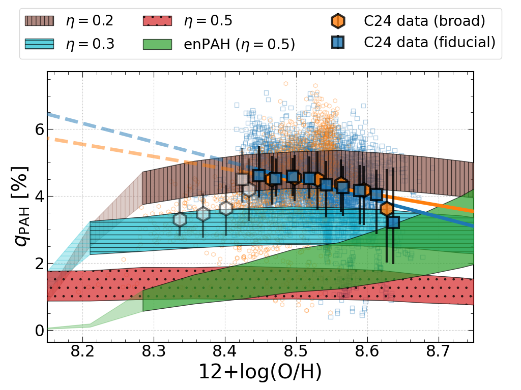
Figure 1: $q_{\mathrm{PAH}}$ as a function of metallicity. The filled blue squares (orange hexagons) show the binned observed data in the fiducial (broad) sample and the lines in the same colour show the linear regression of the corresponding sample. The linear regression only utilizes measurements in the metallicity range where data are complete. The unfilled big hexagons/squares and the dashed lines indicate the region where observed data is not complete. The unfilled small blue squares (orange hexagons) show the pixel-by-pixel observed data in the fiducial (broad) sample. The shaded regions show the model-predicted $q_{\mathrm{PAH}}$, where the lower limit comes from the standard aromatic fraction in H23 and the upper limit is set by an aromatic fraction of 1.0 (corresponding to the maximum PAH prescription). The transparent shaded regions indicate the environment where D/M is less than 90 per cent of the fiducial value (0.48, see Section 3).

The observed $q_{\mathrm{PAH}}$ vs. metallicity trends are compared with the theoretical predictions in Fig. 1. We first discuss the standard models. At low metallicity ($12+\log({\rm O/H})\lesssim 8.3$, depending on $\eta$), the standard models predict low $q_{\mathrm{PAH}}$. This is due to the lack of efficient small grain production by accretion and shattering; however, our observational data is incomplete at such low metallicity ($12+\log({\rm O/H})\lesssim 8.4$) and does not provide a firm comparison. At moderate to high metallicity ($12+\log({\rm O/H})\gtrsim 8.3$, depending on $\eta$), $q_{\mathrm{PAH}}$ is nearly constant in the standard models. This is because the equilibrium between shattering and coagulation for PAHs has been achieved. This is mostly the metallicity regime where robust data are available. The level of equilibrium $q_{\mathrm{PAH}}$ strongly depends on $\eta$ and is higher for smaller $\eta$. Among the standard models, the one with $\eta=0.2$ has its equilibrium $q_{\mathrm{PAH}}$ most consistent with the observation. This is in agreement with our previous results (Hirashita et al., 2020): Lower $\eta$, which enhances the abundance of small grains (including PAHs), is favoured to reproduce the level of PAH emission (Hirashita et al., 2020). This is likely consistent with the observations by Sutter et al. (2024), who found that the strength of PAH emission, relative to other small grain emission, decreases as gas density increases. They raised coagulation as a possible explanation for this decrease. However, the standard model with low $\eta$ does not predict the observed $q_{\mathrm{PAH}}$–metallicity anti-correlation in the fiducial sample, especially at high metallicity. This decreasing trend of $q_{\mathrm{PAH}}$ with metallicity is more consistent with high-$\eta$ models where the enhanced effect of coagulation at high metallicity is more obvious. Due to stronger coagulation in more dust-rich (or metal-rich) regions, one would expect that $q_{\mathrm{PAH}}$ decreases with metallicity (recall that PAHs are depleted by coagulation since they are attached onto larger grains). This decline is rather consistent with high-$\eta$ predictions because of more significant coagulation towards higher metallicity. Thus, the $q_{\mathrm{PAH}}$–metallicity trend may be in favour of high $\eta$ while the absolute level of $q_{\mathrm{PAH}}$ is rather in agreement with low $\eta$. We will explore other explanations for high-metallicity $q_{\mathrm{PAH}}$ decline in Section 5.3.

As mentioned in Section 3, we also examine the enPAH model, which produces a larger $q_{\mathrm{PAH}}$ with a larger $\eta$ $(\simeq 0.5)$ because no PAHs are removed by coagulation (Hirashita, 2023a). However, the enPAH model produces a clearly increasing trend of $q_{\mathrm{PAH}}$ as a function of metallicity, which is not supported by our spatially resolved observational data. Additionally, the absolute $q_{\mathrm{PAH}}$ level is only closer to observations at high metallicity. Previous galaxy-integrated observations do show an increasing trend of $q_{\mathrm{PAH}}$ with metallicity (e.g. Draine et al., 2007; Rémy-Ruyer et al., 2015; Galliano et al., 2018; Aniano et al., 2020). However, that trend is usually more significant when comparing $Z<0.5Z_{\odot}$ galaxies to $Z\sim Z_{\odot}$ ones instead of a smooth increment with metallicity; thus the enPAH model does not necessarily explain their findings, either. We will omit the enPAH model in the following analysis. The unsuccessful results of the enPAH model, which decouple PAHs from interstellar processing (especially coagulation), suggest the balance between coagulation and shattering plays an important role in the flat (or decreasing) trend of $q_{\mathrm{PAH}}$ with metallicity.

4.2 $\alpha_{\rm CO}$ and grain size distribution

Here we discuss the dependence of $\alpha_{\rm CO}$ on grain size distribution. As mentioned at the beginning of this section, we use $q_{\mathrm{PAH}}$ as the indicator for grain size distribution in this work. We show how $\alpha_{\rm CO}$ behaves with metallicity and $q_{\mathrm{PAH}}$ in Fig. 2. Both the observed and model-predicted $\alpha_{\rm CO}$ negatively correlate with metallicity, and the binned observed data falls in the model prediction range. The predicted $\alpha_{\rm CO}$–metallicity relations at different $\eta$ do not differ significantly considering the scatter in observed data. Meanwhile, the large observed scatter of $\alpha_{\rm CO}$ at fixed metallicity is not simply explained by the variation in the grain size distribution, thus physical conditions other than dust evolution, such as gas temperature and velocity dispersion which affect the CO emissivity (e.g. H23 and Teng et al., 2024), should play a role in producing the variation in $\alpha_{\rm CO}$ at a fixed metallicity. We refer readers to the reviews Bolatto et al. (2013) and Schinnerer & Leroy (2024) for the impacts of non-dust evolution mechanisms on $\alpha_{\rm CO}$.

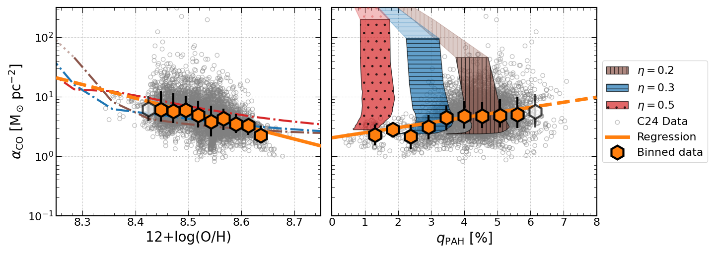
Figure 2: Relation between measured and modeled $\alpha_{\rm CO}$ and physical parameters, metallicity (left) and $q_{\mathrm{PAH}}$ (right). The small empty circles show the distribution of pixel-by-pixel measurements. The orange hexagons show the binned data distribution, while the orange line shows the linear regression of pixel-by-pixel measurements. We show the model prediction from H23 with different values of dense gas fraction in brown, blue and red lines (left panel) or shaded areas (right panel) as shown in the legend.

For the dependence of $\alpha_{\rm CO}$ on $q_{\mathrm{PAH}}$, there is a considerable difference between observed and model-predicted data sets. The observed $\alpha_{\rm CO}$ positively correlates with $q_{\mathrm{PAH}}$. The Spearman’s correlation coefficient ($\rho$) of $\alpha_{\rm CO}$ with $q_{\mathrm{PAH}}$ is 0.21, which is weaker than the ones with metallicity ($\rho=-0.41$) and $r_{\mathrm{g}}/R_{25}$ ($\rho=0.28$), meaning that this correlation between $\alpha_{\rm CO}$ and $q_{\mathrm{PAH}}$ is secondary compared to other correlations. Meanwhile, the model-predicted $q_{\mathrm{PAH}}$ has no clear correlation with $\alpha_{\rm CO}$. As shown in Section 4.1, $q_{\mathrm{PAH}}$ is roughly constant once $\eta$ is set, while $\alpha_{\rm CO}$ still varies with metallicity. Thus, although our model with $\eta=0.2$ broadly explains the $q_{\mathrm{PAH}}$–metallicity and $\alpha_{\rm CO}$–metallicity relations, it does not seem to reproduce the observed $\alpha_{\rm CO}$–$q_{\mathrm{PAH}}$ relation. In other words, the observed $\alpha_{\rm CO}$–$q_{\mathrm{PAH}}$ relation may be caused by mechanisms other than metal/dust enrichment; for example, by the local physical condition (radiation field, gas temperature, etc.). Besides $q_{\mathrm{PAH}}$, H23 predicted that $\alpha_{\rm CO}$ decreases with an increased presence of small dust grains, as stronger dust shielding occurs. However, we observe that $\alpha_{\rm CO}$ increases with $q_{\mathrm{PAH}}$. This could mean that $q_{\mathrm{PAH}}$ does not work well as an indicator for size distribution, or that the observed $\alpha_{\rm CO}$–$q_{\mathrm{PAH}}$ relation is dominated by a mechanism irrelevant to dust evolution.

The above result implies the limitation in our model. Our evolution model of grain size distribution is based on a one-zone treatment where all physical conditions are set to be uniform; thus, it does not consider local physical conditions. Therefore, we also investigate the same relations as above for the galaxy-integrated properties, where local variations are averaged. This is shown in Fig. 3. For the observational data set, we take $\Sigma_{\mathrm{dust}}$-weighted averaged $q_{\mathrm{PAH}}$, $\Sigma_{\mathrm{gas}}$-weighted $12+\log({\rm O/H})$ and $I_{\mathrm{CO}}$-weighted averaged $\alpha_{\rm CO}$.

In the left panel of Fig. 3, we show that the galaxy-integrated $\alpha_{\rm CO}$ still negatively correlates with metallicity, which is consistent with C24. The models are also consistent with the observed $\alpha_{\rm CO}$–metallicity relation. In the right panel, we find that the observed $\alpha_{\rm CO}$–$q_{\mathrm{PAH}}$ pairs of most galaxies fall within the prediction of the $\eta=0.2$ model on the $\alpha_{\rm CO}$–$q_{\mathrm{PAH}}$ plane. A weak correlation between $\alpha_{\rm CO}$ and $q_{\mathrm{PAH}}$ remains, which is not accounted for by our model. Nevertheless, our model successfully reproduces the overall galaxy-integrated $\alpha_{\rm CO}$–$q_{\mathrm{PAH}}$–metallicity relations.

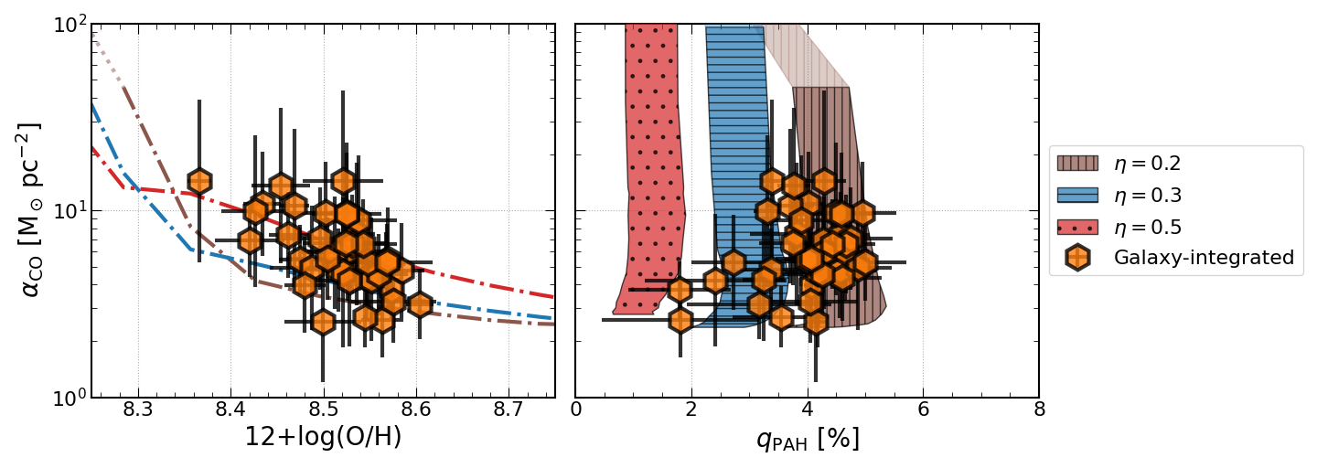
Figure 3: Measured and modelled $\alpha_{\rm CO}$ in terms of metallicity (left) and $q_{\mathrm{PAH}}$ (right) for galaxy-integrated observations. Each orange hexagon represents one observed galaxy. The completeness threshold is not considered for the galaxy-integrated regression. The lines for the model predictions are the same as those shown in Fig. 2.

We do not obtain significant evidence that the grain size distribution affects $\alpha_{\rm CO}$. The positive trend between $\alpha_{\rm CO}$ and $q_{\mathrm{PAH}}$ is opposite to what is expected from the grain size distribution. Indeed, a negative correlation would be expected since large $q_{\mathrm{PAH}}$ would mean more small grains which decrease $\alpha_{\rm CO}$ (H23). The positive correlation likely comes from the negative correlation between $q_{\mathrm{PAH}}$ and metallicity (or dust abundance); that is, if the metallicity (or dust abundance) is high, both $\alpha_{\rm CO}$ and $q_{\mathrm{PAH}}$ are lowered (Sections 4.1 and 4.2), producing a positive correlation between $\alpha_{\rm CO}$ and $q_{\mathrm{PAH}}$. Thus, the effect of dust enrichment (increase in dust abundance) is more prominent than the change in grain size distribution. However, this does not necessarily mean that the effect of grain size distribution is negligible. We further make an effort to extract the signature of grain size distribution in Section 5.2.

5 Discussion

5.1 Alternative indicator for grain size distribution

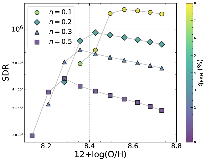
Figure 4: The model-predicted evolution of SDR with metallicity, colourized by $q_{\mathrm{PAH}}$. The symbols show tracks with different $\eta$ as indicated in the legend. As the colour scale indicates, $q_{\mathrm{PAH}}$ traces the variation in SDR with $\eta$, but not the variation at fixed $\eta$.

In Section 4, we used $q_{\mathrm{PAH}}$ as the indicator of dust grain size distribution. This might not be the ultimate solution, as theoretically, $q_{\mathrm{PAH}}$ only accounts for a portion of small carbonaceous grains. Instead of $q_{\mathrm{PAH}}$, the theoretical work H23 used the ratio between the total grain surface area and the total dust mass, SDR, as an indicator of grain size distribution, which better encompasses the overall size distribution. Higher SDR indicates that the grain size distribution is more biased towards smaller sizes. H23 suggested an empirical formula to correct $\alpha_{\rm CO}$ for the grain size distribution using SDR, which is expressed with the conversion from $X_{\mathrm{CO}}$ to $\alpha_{\rm CO}$ as:

$$\alpha_{\rm CO}=4.3\left(\frac{\mathcal{D}}{7\times 10^{-3}}\right)^{-2}\left(\frac{\mathrm{SDR}}{\mathrm{SDR}_{0}}\right)^{-0.5}\,{\rm M_{\odot}\,pc^{-2}\,(K\,km\,s^{-1})^{-1}},$$ (3)

where $\mathcal{D}$ is the dust-to-gas ratio, and $\mathrm{SDR}_{0}=2.9\times 10^{5}~\mathrm{cm^{2}~g^{-1}}$ is a reference SDR. We investigate whether we can find observational correspondence for SDR and then verify this prediction.

We first examine whether $q_{\mathrm{PAH}}$, a quantity shared by observation and model, can be used as an observational correspondence for SDR. In Fig. 4, we show the relation between SDR, $q_{\mathrm{PAH}}$ and metallicity. To the first order, the values of both $q_{\mathrm{PAH}}$ and SDR at high metallicity decrease with $\eta$, which results from the removal of small grains mainly due to coagulation. The variation in SDR is more significant. At lower metallicity, $q_{\mathrm{PAH}}$ is roughly constant at fixed $\eta$; meanwhile, SDR first increases with metallicity then decreases, spanning up to a factor of 2. In other words, we observe that, at fixed $\eta$, one $q_{\mathrm{PAH}}$ value could map to multiple SDR values. Moreover, the typical uncertainty for the observed $q_{\mathrm{PAH}}$ in the z0MGS-Herschel catalogue is $\sim 0.2\%$, which is similar to the predicted span of $q_{\mathrm{PAH}}$ at fixed $\eta$. These facts make $q_{\mathrm{PAH}}$ a suboptimal candidate for serving as the sole tracer for SDR.

We thus move on and examine whether the other quantities shared by the H23 model and C24 observation traces the change of SDR at fixed $\eta$. Since we assume fixed D/M in the observational data, there is practically only one shared observable left, which is metallicity. As shown in Fig. 4, at fixed $\eta$, each metallicity value only maps to one SDR value, which makes it a potential tracer for SDR. On the other hand, metallicity does not catch how SDR varies with $\eta$, which means that we need both $q_{\mathrm{PAH}}$ and metallicity to infer SDR.

Based on the above arguments, we expect that SDR could be expressed by a combination of $q_{\mathrm{PAH}}$ and metallicity. Thus, we interpolate SDR on the $q_{\mathrm{PAH}}$–metallicity 2-dimensional plane. In the interpolation, we used model-predicted values at various $\eta$, omitting the data points at early evolution stages (low metallicity) for smoothness. The resulting interpolation is shown in Fig. 5, and is used to infer SDR values for each observed pixel from their $q_{\mathrm{PAH}}$ and metallicity measurements.

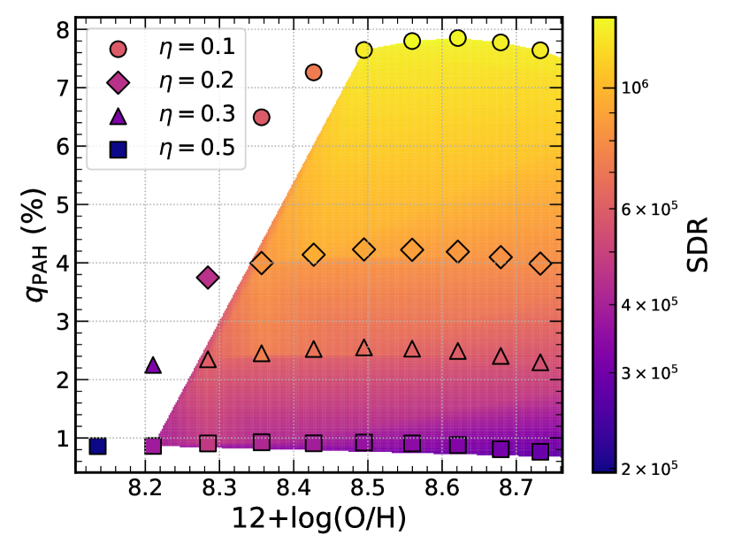
Figure 5: Relation among SDR, $q_{\mathrm{PAH}}$ and metallicity. The symbols show the model-predicted dataset, and the shaded region presents the 2-dimensional interpolation of SDR. We drop the low-metallicity points because we cannot reach a smooth interpolation with them.

5.2 Variation in $\alpha_{\rm CO}$ with SDR

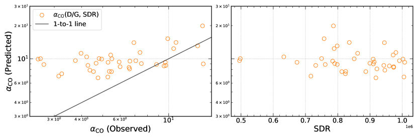
Figure 6: $\alpha_{\rm CO}$ and grain size distribution. Left: $\alpha_{\rm CO}$ predicted as a function of D/G and SDR (equation 18 in H23) versus the galaxy-integrated observations. Right: The predicted $\alpha_{\rm CO}$ versus SDR. There is no obvious trend between $\alpha_{\rm CO}$ and SDR, suggesting that the dependence of $\alpha_{\rm CO}$ on SDR is only secondary.

In Fig. 6 (left panel), we show the $\alpha_{\rm CO}$ values predicted by equation (3), which are compared with the observed $\alpha_{\rm CO}$ in each galaxy. The SDR value is from the interpolation described in Section 5.1. We find a systematic trend of overpredicting $\alpha_{\rm CO}$ at low observed $\alpha_{\rm CO}$. In other words, the $\alpha_{\rm CO}$ values from H23 models have a smaller dynamic range than those from the observations, implying that physical factors other than dust evolution also influence $\alpha_{\rm CO}$ strongly. The overestimating trend at low $\alpha_{\rm CO}$ could be explained by the $\alpha_{\rm CO}$ decline due to increased CO emissivity (e.g. Hayashi et al., 2019; Teng et al., 2024; Chiang et al., 2024; Schinnerer & Leroy, 2024), which is not taken into account in the H23 model. Recent studies on the molecular clouds in the MW and Large Magellanic Cloud also showed that $\alpha_{\rm CO}$ could vary by almost an order of magnitude at fixed metallicity (Kohno & Sofue, 2024b, a; Li et al., 2024), This is consistent with the arguments in Section 4.2 based on the $\alpha_{\rm CO}$–$q_{\mathrm{PAH}}$ relation.

To further understand the prediction with the dust evolution mechanisms only, we examine the components in equation (3): the total dust abundance (D/G) term and the grain size distribution (SDR) term. The D/G term is broadly consistent with literature values (e.g. Schruba et al., 2012; Bolatto et al., 2013; Hunt et al., 2015; Accurso et al., 2017; Schinnerer & Leroy, 2024); thus, we focus on the SDR term. In order to examine the effect of SDR, we first show in Fig. 6 (right panel) the $\alpha_{\rm CO}$ values predicted from equation (3) in terms of SDR. We do not find any significant trend. This indicates that the impact of grain size distribution on $\alpha_{\rm CO}$ is secondary compared to other mechanisms among the sample galaxies. However, the above result does not indicate that the grain size distribution is unimportant. It is fair to say that the dynamic range of SDR is small compared with other quantities affecting $\alpha_{\rm CO}$ at galaxy-integrated scales because the grain size distribution is converged to a functional shape determined by the balance between coagulation and shattering as we argued in Section 4.1.

5.3 Alternative explanations of high-metallicity $q_{\mathrm{PAH}}$ decline

In Section 4, we focused on coagulation in the discussion on PAH destruction mechanisms, especially at high metallicity, and neglected other possibilities, e.g. photodestruction of PAHs in hard radiation fields or weaker PAH emission with softer radiation in the bulge. We will discuss these two cases here.

5.3.1 Photodestruction of PAHs

Since the chemical structure of astronomical PAHs is not unique, we make a rough calculation of the energy required to dissociate a single bond in a benzene ring, the building block of PAHs. A rough calculation of the dissociation energy includes the C–C bond, the C=C bond and the resonance energy. The average bond energy of C–C and C=C bonds are 347 and 614 kJ mol^-1, respectively. The resonance energy of a benzene ring is 150 kJ mol^-1. Thus, to photodissociate a single bond in a benzene ring, a photon with an energy of at least 5.27 eV ($\lambda\sim 235$ nm) is required. Kislov et al. (2004) calculated the probability of various pathways of photodissociation of benzene at different wavelengths. They found that the dissociation of H atoms starts to occur at $\lambda\lesssim 193$ nm. They also predicted that the dissociation of C atoms might be observable at $\lambda\leq 157$ nm. Thus, it seems possible to observe the photodestruction of PAHs under a hard radiation field. Murga et al. (2019) calculated the PAH photodestruction time-scale as a function of ISRF strength. According to their calculation, the ISRFs in our dataset ($\log\overline{U}\lesssim 1.5$) would predict PAH destruction of $\gtrsim 10^{9}~\mathrm{yr}$, which is less efficient than the reference coagulation time-scale of $\gtrsim 10^{7}~\mathrm{yr}$ (Hirashita & Yan, 2009). Thus although photodestruction of PAHs is possible in our sample, it is expected to be less efficient than the processes included in our models.

Besides theoretical works, previous observations have found evidence of PAHs being destroyed by strong radiation fields. For example, Chastenet et al. (2019) showed that the destruction of PAHs, indicated by local $q_{\mathrm{PAH}}$ relative to the average $q_{\mathrm{PAH}}$ in each of their sample galaxies (the Magellanic Clouds), strongly correlates with the surface brightness of H$\alpha$ at 10 pc scale. They also showed that in the diffuse neutral medium, it is not clear whether the ISRF strength impacts the destruction of PAHs. Studies with Spitzer IRAC photometry (Khramtsova et al., 2013) and recent (sub-)cloud scale studies with JWST also showed lowered $q_{\mathrm{PAH}}$ in H ii regions (Chastenet et al., 2023; Egorov et al., 2023).

Meanwhile, this work examines $\sim$kpc scales, focusing on neutral gas-dominated environments. Therefore, we need to carefully interpret sub-cloud scale findings in H ii regions for our analysis. Sutter et al. (2024) used PHANGS-JWST observations and conducted several tests about how PAH band ratio ($R_{\mathrm{PAH}}\equiv\mathrm{[F770W+F1130W]/F2100W}$, which traces $q_{\mathrm{PAH}}$) varies depending on averaging methods. First, they confirmed that $R_{\mathrm{PAH}}$ is systematically lower in H ii regions compared to diffuse regions at 10–50 pc scales. However, this effect is only significant when $R_{\mathrm{PAH}}$ is calculated as H$\alpha$-weighted average. When they took simple averages over larger regions, there is no significant difference in $R_{\mathrm{PAH}}$ between diffuse and H ii regions, indicating that the photodestruction effect is easily diluted when working at coarser resolution. They then investigated whether $R_{\mathrm{PAH}}$ is affected by the presence of H ii regions in kpc-scale cells, and they did not find a significant trend of $R_{\mathrm{PAH}}$ with the percentage of pixels identified as H ii regions. In summary, photodestruction of PAHs is theoretically possible and effective on much smaller scales than our adopted resolution ($\sim$kpc). Thus, it is unlikely that the decreasing trend of $q_{\mathrm{PAH}}$ with metallicity presented in Section 4 is due to photodestruction.

5.3.2 Bulge correction for $q_{\mathrm{PAH}}$

The rate at which starlight heats dust differs with the starlight spectrum at a fixed mean ISRF strength ($\overline{U}$). This effect impacts small grains more than large grains, causing possible misestimate of $q_{\mathrm{PAH}}$ from the SED fitting when the starlight spectrum is different from the model assumption, e.g. when $\overline{U}$ is dominated by the older stellar population in the bulge (Draine et al., 2014; Whitcomb et al., 2024). Draine et al. (2014) provided a detailed strategy for correcting the underestimated $q_{\mathrm{PAH}}$ when $\overline{U}$ consists of the bulge ISRF ($U_{\mathrm{bulge}}$) and the disc ISRF ($U_{\mathrm{disc}}$). However, the derivation of $U_{\mathrm{bulge}}$ requires robust measurements of bulge core radius for all our sample galaxies, which is beyond the scope of this work. Thus, we do not include this correction in our fiducial analysis.

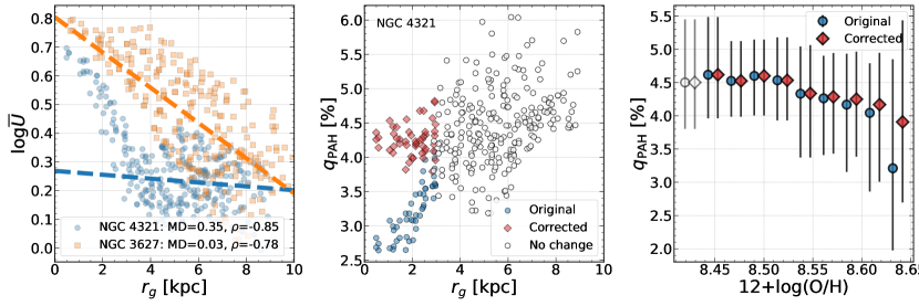
Figure 7: Left: Pixel-by-pixel $\overline{U}$ as a function of $r_{\mathrm{g}}$ in two example galaxies (orange circles and blue squares for NGC 4321 and NGC 3627, respectively). The dashed lines show the exponential disc fits ($U_{\mathrm{disc}}$) for each galaxy with corresponding colours. In NGC 4321, we could extract $U_{\mathrm{bulge}}$, while in NGC 3627, we could not extract $U_{\mathrm{bulge}}$ because of the small deviation between $\overline{U}$ and the extrapolated disc component in the inner galaxy. Middle: Pixel-by-pixel corrected $q_{\mathrm{PAH}}$ compared to original $q_{\mathrm{PAH}}$ as a function of $r_{g}$ in NGC 4321. The empty circles show where $q_{\mathrm{PAH}}$ remains the same. Right: Binned corrected $q_{\mathrm{PAH}}$ compared to original $q_{\mathrm{PAH}}$ as a function of metallicity. The errorbar shows the 16th and 84th percentiles in each bin. The empty symbols present data outside the completeness cut.

Here, we use a simplified strategy to estimate the impact from $U_{\mathrm{bulge}}$, inspired by the “scale-down” strategy in Draine et al. (2014) and the “flat $U_{\mathrm{disc}}$” strategy in Whitcomb et al. (2024). The key assumptions in our strategy are: (a) $\overline{U}=U_{\mathrm{bulge}}+U_{\mathrm{disc}}$, where $U_{\mathrm{disc}}$ dominates beyond a certain galactocentric distance ($r_{\mathrm{g}}$); (b) in each galaxy, $U_{\mathrm{disc}}(r_{\mathrm{g}})\propto\mathrm{exp}(-r_{\mathrm{g}}/r_{\mathrm{d}})$, where $r_{\mathrm{d}}$ is a galaxy-dependent scale length of the disc.

In each galaxy, we first fit $\overline{U}$ to $U_{\mathrm{disc}}(r_{g})$ at $r_{g}>3~\mathrm{kpc}$. We then extrapolate the fitted $U_{\mathrm{disc}}(r_{g})$ to the inner galaxy, and calculate $U_{\mathrm{bulge}}=\overline{U}-U_{\mathrm{disc}}$. We take galaxies that meet the following criteria to have a significant bulge component for our analysis: (a) the median deviation (MD) between log$\overline{U}$ and $\log U_{\mathrm{disc}}$ in the inner 2 kpc exceeds 0.1 dex, and (b) the Spearman’s correlation ($\rho$) between $U_{\mathrm{bulge}}$ and $r_{g}$ in the inner 2 kpc is stronger than $-0.5$, with a $p$-value below 0.05. We end up with 6 galaxies satisfying the above criteria: IC 342, NGC 3184, NGC 4051, NGC 4321, NGC 5457 and NGC 6946. Lastly, we adopt equation (21) in Draine et al. (2014) to calculate corrected $q_{\mathrm{PAH}}$. Overall, the median of increase in $q_{\mathrm{PAH}}$ after the correction is 1.12 per cent.

We show some example galaxies and the resulting corrected $q_{\mathrm{PAH}}$ in Fig. 7. In the left panel, we show the $\overline{U}$ (symbols) and fitted $U_{\mathrm{disc}}$ (dashed lines) in two galaxies. NGC 4321 satisfies both criteria, while NGC 3627 does not show large enough MD to extract $U_{\mathrm{bulge}}$. In the middle panel of Fig. 7, we show the corrected and original $q_{\mathrm{PAH}}$ in NGC 4321 as an example. This correction impacts $q_{\mathrm{PAH}}$ at $r_{\mathrm{g}}\lesssim 3~\mathrm{kpc}$ depending on how $\overline{U}$ behaves with $r_{g}$ and where we fit $U_{\mathrm{disc}}(r_{g})$. The corrected $q_{\mathrm{PAH}}$ significantly removes the decline of $q_{\mathrm{PAH}}$ in the inner galaxy shown with the original measurements. The median increase in $q_{\mathrm{PAH}}$ is 0.64 per cent for NGC 4321. In the right panel of Fig. 7, we show how corrected and original $q_{\mathrm{PAH}}$ vary with metallicity for all galaxies, in a manner similar to Fig. 1 (fiducial sample). In the highest metallicity bin, $q_{\mathrm{PAH}}$ rises by almost 1 per cent after the correction, while the other bins are barely affected. In summary, the correction for the bulge radiation field increases the $q_{\mathrm{PAH}}$ values only in the innermost (highest-metallicity) part of galaxies. It weakens the negative trend of $q_{\mathrm{PAH}}$ with metallicity but does not remove it. Thus, we conclude that the different stellar populations in high-metallicity regions do not significantly affect the observationally derived $q_{\mathrm{PAH}}$–metallicity relation.

6 Summary

We investigate how grain size distribution affects the CO-to-H₂ conversion factor ($\alpha_{\rm CO}$) and how the PAH fraction ($q_{\mathrm{PAH}}$), which is used as an indicator of grain size distribution, evolves with local environments with both observations and models. We adopt the C24 measurements of $\alpha_{\rm CO}$, metallicity, and $q_{\mathrm{PAH}}$ at 2 kpc resolution in 42 nearby galaxies. The $\alpha_{\rm CO}$ is derived from measured $W_{\mathrm{CO}}$, $\Sigma_{\mathrm{dust}}$, $\Sigma_{\mathrm{atom}}$ and metallicity assuming $\mathrm{D/M}=0.48$. The dust properties are derived from the IR SED fitting with the Draine & Li (2007) model as part of the z0MGS-Herschel work (Chastenet et al., 2024). We utilize the H23 analytical model that calculates $\alpha_{\rm CO}$ in a manner consistent with the evolution of dust abundance and grain size distribution. It is capable of predicting $\alpha_{\rm CO}$, D/G, metallicity, $q_{\mathrm{PAH}}$ and SDR at each evolutionary stage.

We find a weak anti-correlation between the observed $q_{\mathrm{PAH}}$ and metallicity, especially at $12+\log({\rm O/H})>8.4$. This anti-correlation is stronger in CO-bright environments. Meanwhile, the H23 models predict a roughly constant $q_{\mathrm{PAH}}$ at mid- to high-metallicity at fixed $\eta$ (dense gas fraction), which is more consistent with the broad sample (omitting S/N cuts). On the other hand, the equilibrium $q_{\mathrm{PAH}}$ is set by the balance between shattering and coagulation. Lower $\eta$ values yield higher equilibrium $q_{\mathrm{PAH}}$ due to weaker coagulation (or stronger shattering), and the $\eta=0.2$ prediction best matches our observations. The enPAH model, which assumes no coagulation for PAHs, does not align with observed trends. This suggests an important role of coagulation in reproducing the observed $q_{\mathrm{PAH}}$–metallicity relation.

We discuss how dust properties could impact $\alpha_{\rm CO}$. We first compare the observed and modelled $\alpha_{\rm CO}$ and examine the dependence on metallicity and $q_{\mathrm{PAH}}$. The observations and the model predictions show similar anti-correlation between $\alpha_{\rm CO}$ and metallicity, while the observations have a larger span of $\alpha_{\rm CO}$ at fixed metallicity than explained by the models. Meanwhile, the observations and the models show a considerable difference in the $\alpha_{\rm CO}$–$q_{\mathrm{PAH}}$ relation. The observed $\alpha_{\rm CO}$ shows a positive correlation with $q_{\mathrm{PAH}}$, whereas the model-predicted $\alpha_{\rm CO}$ lacks a clear correlation with $q_{\mathrm{PAH}}$. On the other hand, galaxy-integrated observations show consistent results with the predictions, indicating that the discrepancy we show in the pixel-by-pixel analysis is likely due to the limitation arising from the one-zone treatment in the model.

We also investigate how $\alpha_{\rm CO}$ depends on SDR, the ratio between the total grain surface area and the total dust mass, which is an alternative tracer of grain size distribution adopted by H23. We first examine the relation between SDR and observed quantities and find that $q_{\mathrm{PAH}}$ traces the variation of SDR with $\eta$. However, because of the uncertainty level and the lack of a one-to-one mapping, $q_{\mathrm{PAH}}$ does not trace the evolution of SDR at fixed $\eta$. Meanwhile, we find a one-to-one mapping from metallicity to SDR at fixed $\eta$. With the combination of $q_{\mathrm{PAH}}$ and metallicity, we build a 2-dimensional interpolation map to assign SDR values to observational data. We find that the $\alpha_{\rm CO}$ predicted from SDR and metallicity with the formula derived in H23 is more consistent with the observations at larger $\alpha_{\rm CO}$ values. While SDR affects $\alpha_{\rm CO}$, the impact of the SDR term to $\alpha_{\rm CO}$ value is secondary compared to other physical conditions in the ISM, e.g. the $\alpha_{\rm CO}$ decline due to increased CO emissivity.

We discuss the possible reasons for the $q_{\mathrm{PAH}}$ decline at high metallicity besides coagulation. PAHs could be destroyed by hard radiation fields in H ii regions. However, this effect is likely unobservable at our 2 kpc resolution. The bulge ISRF correction could raise $q_{\mathrm{PAH}}$ at near solar metallicity by almost 1 per cent from our estimation. However, this effect alone does not explain the negative $q_{\mathrm{PAH}}$–metallicity correlation. Given that the above two mechanisms do not completely explain this negative correlation, coagulation remains a viable process that naturally explains the decrease of $q_{\mathrm{PAH}}$ with metallicity.

Data Availability

Data related to this publication and its figures are available on reasonable request from the corresponding author.

Appendix A Galaxy samples

We present the properties of galaxies studies in this work and the references for adopted data in Table 1.

Table 1: Galaxy Sample.

Galaxy	Dist.	$i$	P.A.	$R_{25}$	$R_{e}$	$\log(M_{\star})$	Type	CO $(1{\scalebox{0.75}[1.0]{$-$}}0)$	CO $(2{\scalebox{0.75}[1.0]{$-$}}1)$	H i 21 cm Ref	12+log(O/H) Ref
	[Mpc]	[′]	[′]	[kpc]	[kpc]	[M⊙]
(1)	(2)	(3)	(4)	(5)	(6)	(7)	(8)	(9)	(10)	(11)	(12)
IC 342	3.5	31.0	42.0	10.1	4.4	10.2	5	CO Atlas	$~\cdots~$	EveryTHINGS	$f.$
NGC 253	3.7	75.0	52.5	14.4	4.7	10.5	5	CO Atlas	PHANGS-ALMA	$c.$	$g.$
NGC 300	2.1	39.8	114.3	5.9	2.0	9.3	6	$~\cdots~$	PHANGS-ALMA	$d.$	$h.$
NGC 598	0.9	55.0	201.0	8.1	2.4	9.4	5	$~\cdots~$	$a.$	$e.$	$h.$
NGC 628	9.8	8.9	20.7	14.1	3.9	10.2	5	COMING	PHANGS-ALMA	THINGS	PHANGS-MUSE
NGC 925*	9.2	66.0	287.0	14.3	4.5	9.8	6	$~\cdots~$	HERACLES	THINGS	$h.$
NGC 2403*	3.2	63.0	124.0	9.3	2.4	9.6	5	$~\cdots~$	HERACLES	THINGS	$h.$
NGC 2841	14.1	74.0	153.0	14.2	5.4	10.9	3	COMING	$~\cdots~$	THINGS	$g.$
NGC 2976*	3.6	65.0	335.0	3.0	1.3	9.1	5	COMING	HERACLES	THINGS	$g.$
NGC 3184	12.6	16.0	179.0	13.6	5.3	10.3	5	CO Atlas	HERACLES	THINGS	$h.$
NGC 3198	13.8	72.0	215.0	13.0	5.0	10.0	5	COMING	HERACLES	THINGS	$g.$
NGC 3351	10.0	45.1	193.2	10.5	3.1	10.3	3	CO Atlas	PHANGS-ALMA	THINGS	PHANGS-MUSE
NGC 3521	13.2	68.8	343.0	16.0	3.9	11.0	3	CO Atlas	PHANGS-ALMA	THINGS	$g.$
NGC 3596	11.3	25.1	78.4	6.0	1.6	9.5	5	$~\cdots~$	PHANGS-ALMA	EveryTHINGS	$g.$
NGC 3621	7.1	65.8	343.8	9.9	2.7	10.0	6	$~\cdots~$	PHANGS-ALMA	THINGS	$h.$
NGC 3627	11.3	57.3	173.1	16.9	3.6	10.7	3	CO Atlas	PHANGS-ALMA	THINGS	PHANGS-MUSE
NGC 3631	18.0	32.4	-65.6	9.7	2.9	10.2	5	CO Atlas	$b.$	EveryTHINGS	$g.$
NGC 3938	17.1	14.0	195.0	13.4	3.7	10.3	5	COMING	HERACLES	HERACLES-VLA	$g.$
NGC 3953	17.1	61.5	12.5	15.2	5.3	10.6	4	$~\cdots~$	$b.$	EveryTHINGS	$g.$
NGC 4030	19.0	27.4	28.7	10.5	2.1	10.6	4	COMING	$~\cdots~$	EveryTHINGS	$g.$
NGC 4051	17.1	43.4	-54.8	14.7	3.7	10.3	3	CO Atlas	$b.$	EveryTHINGS	$g.$
NGC 4207	15.8	64.5	121.9	3.5	1.4	9.6	7	$~\cdots~$	PHANGS-ALMA	PHANGS-VLA	$g.$
NGC 4254	13.1	34.4	68.1	9.6	2.4	10.3	5	CO Atlas	PHANGS-ALMA	HERACLES-VLA	PHANGS-MUSE
NGC 4258	7.6	68.3	150.0	18.8	5.9	10.7	4	COMING	$~\cdots~$	HALOGAS	$h.$
NGC 4321	15.2	38.5	156.2	13.5	5.5	10.7	3	CO Atlas	PHANGS-ALMA	HERACLES-VLA	PHANGS-MUSE
NGC 4450	16.8	48.5	-6.3	13.3	4.3	10.7	2	$~\cdots~$	$b.$	EveryTHINGS	$g.$
NGC 4496A*	14.9	53.8	51.1	7.3	3.0	9.6	6	$~\cdots~$	PHANGS-ALMA	EveryTHINGS	$g.$
NGC 4501	16.8	60.1	-37.8	21.1	5.2	11.0	3	CO Atlas	$~\cdots~$	EveryTHINGS	$g.$
NGC 4536	16.2	66.0	305.6	16.7	4.4	10.2	3	CO Atlas	PHANGS-ALMA	HERACLES-VLA	$g.$
NGC 4569	15.8	70.0	18.0	21.0	5.9	10.8	2	CO Atlas	PHANGS-ALMA	HERACLES-VLA	$g.$
NGC 4625	11.8	47.0	330.0	2.4	1.2	9.1	9	$~\cdots~$	HERACLES	HERACLES-VLA	$h.$
NGC 4651	16.8	50.1	73.8	9.5	2.4	10.3	5	$~\cdots~$	$b.$	EveryTHINGS	$h.$
NGC 4689	15.0	38.7	164.1	8.3	4.7	10.1	5	CO Atlas	PHANGS-ALMA	EveryTHINGS	$g.$
NGC 4725	12.4	54.0	36.0	17.5	6.0	10.8	1	$~\cdots~$	HERACLES	HERACLES-VLA	$g.$
NGC 4736	4.4	41.0	296.0	5.0	0.8	10.3	1	CO Atlas	HERACLES	THINGS	$g.$
NGC 4941	15.0	53.4	202.2	7.3	3.4	10.1	1	$~\cdots~$	PHANGS-ALMA	EveryTHINGS	$g.$
NGC 5055	9.0	59.0	102.0	15.5	4.2	10.7	4	CO Atlas	HERACLES	THINGS	$g.$
NGC 5248	14.9	47.4	109.2	8.8	3.2	10.3	3	CO Atlas	PHANGS-ALMA	PHANGS-VLA	$g.$
NGC 5457	6.7	18.0	39.0	23.4	13.5	10.3	5	CO Atlas	HERACLES	THINGS	$h.$
NGC 6946	7.3	33.0	243.0	12.1	4.4	10.5	5	CO Atlas	HERACLES	THINGS	$h.$
NGC 7331	14.7	76.0	168.0	19.8	3.7	11.0	4	COMING	HERACLES	THINGS	$g.$
NGC 7793*	3.6	50.0	290.0	5.4	1.9	9.3	6	$~\cdots~$	PHANGS-ALMA	THINGS	$h.$

• Notes: (1) Name of galaxies. We mark the galaxies not presented in C24 with “*”; (2) Distance (from EDD Tully et al., 2009); (3-4) inclination angle and position angle (Sofue et al., 1999; de Blok et al., 2008; Leroy et al., 2009; Muñoz-Mateos et al., 2009; Meidt et al., 2009; McCormick et al., 2013; Makarov et al., 2014; Lang et al., 2020); (5) isophotal radius (Makarov et al., 2014); (6) effective radius (Leroy et al., 2021); (7) logarithmic global stellar mass (Leroy et al., 2019); (8) numerical Hubble stage T; (9) References of CO $J=1\to 0$ observations (“$~\cdots~$” means no CO $J=1\to 0$ data adopted in this work): CO Atlas Kuno et al. (2007); COMING (Sorai et al., 2019); (10) References of CO $J=2\to 1$ observations (“$~\cdots~$” means no CO $J=2\to 1$ data adopted in this work): HERACLES Leroy et al. (2009); PHANGS-ALMA (Leroy et al., 2021); $a.$ M33 data from Gratier et al. (2010); Druard et al. (2014); $b.$ New HERA data (P.I.: A. Schruba; presented in Leroy et al., 2022); (11) References of Hi observations: THINGS (Walter et al., 2008); HALOGAS (Heald et al., 2011); HERACLES-VLA (Schruba et al., 2011); PHANGS-VLA (P.I. D. Utomo; I. Chiang et al. in preparation); EveryTHINGS (P.I. K. M. Sandstrom; presented in C24); $c.$ Puche et al. (1991); $d.$ Puche et al. (1990); $e.$ Koch et al. (2018); (12) References of $12+\log({\rm O/H})$ measurement: PHANGS-MUSE (Emsellem et al., 2022; Santoro et al., 2022); $f.$ private communication with K. Kreckel (see Chiang et al., 2021); $g.$ using the empirical formula described in C24; $h.$ data from Zurita et al. (2021) compilation.

References

- Accurso et al. (2017) Accurso G., et al., 2017, MNRAS, 470, 4750
- Aniano et al. (2020) Aniano G., et al., 2020, ApJ, 889, 150
- Arimoto et al. (1996) Arimoto N., Sofue Y., Tsujimoto T., 1996, PASJ, 48, 275
- Asano et al. (2013) Asano R. S., Takeuchi T. T., Hirashita H., Nozawa T., 2013, MNRAS, 432, 637
- Asplund et al. (2009) Asplund M., Grevesse N., Sauval A. J., Scott P., 2009, ARA&A, 47, 481
- Astropy Collaboration et al. (2013) Astropy Collaboration et al., 2013, A&A, 558, A33
- Astropy Collaboration et al. (2018) Astropy Collaboration et al., 2018, AJ, 156, 123
- Astropy Collaboration et al. (2022) Astropy Collaboration et al., 2022, ApJ, 935, 167
- Belfiore et al. (2023) Belfiore F., et al., 2023, A&A, 670, A67
- Bolatto et al. (2013) Bolatto A. D., Wolfire M., Leroy A. K., 2013, ARA&A, 51, 207
- Boulanger et al. (1996) Boulanger F., Abergel A., Bernard J. P., Burton W. B., Desert F. X., Hartmann D., Lagache G., Puget J. L., 1996, A&A, 312, 256
- Chastenet et al. (2019) Chastenet J., et al., 2019, ApJ, 876, 62
- Chastenet et al. (2021) Chastenet J., et al., 2021, ApJ, 912, 103
- Chastenet et al. (2023) Chastenet J., et al., 2023, ApJ, 944, L11
- Chastenet et al. (2024) Chastenet J., et al., 2024, arXiv e-prints, p. arXiv:2410.03835
- Chen et al. (2018) Chen L.-H., Hirashita H., Hou K.-C., Aoyama S., Shimizu I., Nagamine K., 2018, MNRAS, 474, 1545
- Chiang et al. (2021) Chiang I.-D., et al., 2021, ApJ, 907, 29
- Chiang et al. (2024) Chiang I.-D., et al., 2024, ApJ, 964, 18
- de Blok et al. (2008) de Blok W. J. G., Walter F., Brinks E., Trachternach C., Oh S.-H., Kennicutt R. C., 2008, AJ, 136, 2648
- Downes & Solomon (1998) Downes D., Solomon P. M., 1998, ApJ, 507, 615
- Downes et al. (1993) Downes D., Solomon P. M., Radford S. J. E., 1993, ApJ, 414, L13
- Draine & Li (2007) Draine B. T., Li A., 2007, ApJ, 657, 810
- Draine et al. (2007) Draine B. T., et al., 2007, ApJ, 663, 866
- Draine et al. (2014) Draine B. T., et al., 2014, ApJ, 780, 172
- Druard et al. (2014) Druard C., et al., 2014, A&A, 567, A118
- Egorov et al. (2023) Egorov O. V., et al., 2023, ApJ, 944, L16
- Emsellem et al. (2022) Emsellem E., et al., 2022, A&A, 659, A191
- Feldmann et al. (2012) Feldmann R., Gnedin N. Y., Kravtsov A. V., 2012, ApJ, 747, 124
- Galliano et al. (2018) Galliano F., Galametz M., Jones A. P., 2018, ARA&A, 56, 673
- Glover & Mac Low (2011) Glover S. C. O., Mac Low M. M., 2011, MNRAS, 412, 337
- Gordon et al. (2014) Gordon K. D., et al., 2014, ApJ, 797, 85
- Gratier et al. (2010) Gratier P., et al., 2010, A&A, 522, A3
- Grenier et al. (2005) Grenier I. A., Casandjian J.-M., Terrier R., 2005, Science, 307, 1292
- Groves et al. (2023) Groves B., et al., 2023, MNRAS, 520, 4902
- Hayashi et al. (2019) Hayashi K., Okamoto R., Yamamoto H., Hayakawa T., Tachihara K., Fukui Y., 2019, ApJ, 878, 131
- Heald et al. (2011) Heald G., et al., 2011, A&A, 526, A118
- Herrero-Illana et al. (2019) Herrero-Illana R., et al., 2019, A&A, 628, A71
- Hirashita (2023a) Hirashita H., 2023a, MNRAS, 518, 3827
- Hirashita (2023b) Hirashita H., 2023b, MNRAS, 522, 4612
- Hirashita & Aoyama (2019) Hirashita H., Aoyama S., 2019, MNRAS, 482, 2555
- Hirashita & Harada (2017) Hirashita H., Harada N., 2017, MNRAS, 467, 699
- Hirashita & Murga (2020) Hirashita H., Murga M. S., 2020, MNRAS, 492, 3779
- Hirashita & Yan (2009) Hirashita H., Yan H., 2009, MNRAS, 394, 1061
- Hirashita et al. (2020) Hirashita H., Deng W., Murga M. S., 2020, MNRAS, 499, 3046
- Hunt et al. (2015) Hunt L. K., et al., 2015, A&A, 583, A114
- Israel (1997) Israel F. P., 1997, A&A, 328, 471
- Israel (2009a) Israel F. P., 2009a, A&A, 493, 525
- Israel (2009b) Israel F. P., 2009b, A&A, 506, 689
- Israel (2020) Israel F. P., 2020, A&A, 635, A131
- Issa et al. (1990) Issa M. R., MacLaren I., Wolfendale A. W., 1990, A&A, 236, 237
- Jiao et al. (2021) Jiao Q., Gao Y., Zhao Y., 2021, MNRAS, 504, 2360
- Khramtsova et al. (2013) Khramtsova M. S., Wiebe D. S., Boley P. A., Pavlyuchenkov Y. N., 2013, MNRAS, 431, 2006
- Khramtsova et al. (2014) Khramtsova M. S., Wiebe D. S., Lozinskaya T. A., Egorov O. V., 2014, MNRAS, 444, 757
- Kislov et al. (2004) Kislov V. V., Nguyen T. L., Mebel A. M., Lin S. H., Smith S. C., 2004, J. Chem. Phys., 120, 7008
- Koch et al. (2018) Koch E. W., et al., 2018, MNRAS, 479, 2505
- Kohno & Sofue (2024a) Kohno M., Sofue Y., 2024a, PASJ, 76, 579
- Kohno & Sofue (2024b) Kohno M., Sofue Y., 2024b, MNRAS, 527, 9290
- Kuno et al. (2007) Kuno N., et al., 2007, PASJ, 59, 117
- Lang et al. (2020) Lang P., et al., 2020, ApJ, 897, 122
- Lee et al. (1996) Lee H. H., Herbst E., Pineau des Forets G., Roueff E., Le Bourlot J., 1996, A&A, 311, 690
- Leroy et al. (2009) Leroy A. K., et al., 2009, AJ, 137, 4670
- Leroy et al. (2011) Leroy A. K., et al., 2011, ApJ, 737, 12
- Leroy et al. (2019) Leroy A. K., et al., 2019, ApJS, 244, 24
- Leroy et al. (2021) Leroy A. K., et al., 2021, ApJS, 257, 43
- Leroy et al. (2022) Leroy A. K., et al., 2022, ApJ, 927, 149
- Li (2020) Li A., 2020, Nature Astronomy, 4, 339
- Li et al. (2024) Li Q., Li M., Zhang L., Pei S., 2024, Universe, 10, 200
- Madden et al. (2020) Madden S. C., et al., 2020, A&A, 643, A141
- Makarov et al. (2014) Makarov D., Prugniel P., Terekhova N., Courtois H., Vauglin I., 2014, A&A, 570, A13
- Martin et al. (2005) Martin D. C., et al., 2005, ApJ, 619, L1
- Matsumoto et al. (2024) Matsumoto K., et al., 2024, A&A, 689, A79
- McCormick et al. (2013) McCormick A., Veilleux S., Rupke D. S. N., 2013, ApJ, 774, 126
- Meidt et al. (2009) Meidt S. E., Rand R. J., Merrifield M. R., 2009, ApJ, 702, 277
- Muñoz-Mateos et al. (2009) Muñoz-Mateos J. C., et al., 2009, ApJ, 703, 1569
- Murga et al. (2019) Murga M. S., Wiebe D. S., Sivkova E. E., Akimkin V. V., 2019, MNRAS, 488, 965
- Narayanan et al. (2011) Narayanan D., Krumholz M., Ostriker E. C., Hernquist L., 2011, MNRAS, 418, 664
- Okamoto et al. (2017) Okamoto R., Yamamoto H., Tachihara K., Hayakawa T., Hayashi K., Fukui Y., 2017, ApJ, 838, 132
- Papadopoulos et al. (2002) Papadopoulos P. P., Thi W. F., Viti S., 2002, ApJ, 579, 270
- Papadopoulos et al. (2012) Papadopoulos P. P., van der Werf P. P., Xilouris E. M., Isaak K. G., Gao Y., Mühle S., 2012, MNRAS, 426, 2601
- Pilbratt et al. (2010) Pilbratt G. L., et al., 2010, A&A, 518, L1
- Pilyugin & Grebel (2016) Pilyugin L. S., Grebel E. K., 2016, MNRAS, 457, 3678
- Planck Collaboration et al. (2011) Planck Collaboration et al., 2011, A&A, 536, A19
- Puche et al. (1990) Puche D., Carignan C., Bosma A., 1990, AJ, 100, 1468
- Puche et al. (1991) Puche D., Carignan C., van Gorkom J. H., 1991, AJ, 101, 456
- Rémy-Ruyer et al. (2015) Rémy-Ruyer A., et al., 2015, A&A, 582, A121
- Sánchez et al. (2014) Sánchez S. F., et al., 2014, A&A, 563, A49
- Sánchez et al. (2019) Sánchez S. F., et al., 2019, MNRAS, 484, 3042
- Sandstrom et al. (2013) Sandstrom K. M., et al., 2013, ApJ, 777, 5
- Santoro et al. (2022) Santoro F., et al., 2022, A&A, 658, A188
- Schinnerer & Leroy (2024) Schinnerer E., Leroy A. K., 2024, ARA&A, 62, 369
- Schruba et al. (2011) Schruba A., et al., 2011, AJ, 142, 37
- Schruba et al. (2012) Schruba A., et al., 2012, AJ, 143, 138
- Shivaei et al. (2024) Shivaei I., et al., 2024, A&A, 690, A89
- Smith et al. (2007) Smith J. D. T., et al., 2007, ApJ, 656, 770
- Sofue & Kohno (2020) Sofue Y., Kohno M., 2020, MNRAS, 497, 1851
- Sofue et al. (1999) Sofue Y., Tutui Y., Honma M., Tomita A., Takamiya T., Koda J., Takeda Y., 1999, ApJ, 523, 136
- Sorai et al. (2019) Sorai K., et al., 2019, PASJ, 71, S14
- Sun et al. (2020) Sun J., et al., 2020, ApJ, 892, 148
- Sutter et al. (2024) Sutter J., et al., 2024, ApJ, 971, 178
- Teng et al. (2022) Teng Y.-H., et al., 2022, ApJ, 925, 72
- Teng et al. (2023) Teng Y.-H., et al., 2023, ApJ, 950, 119
- Teng et al. (2024) Teng Y.-H., et al., 2024, ApJ, 961, 42
- Tully et al. (2009) Tully R. B., Rizzi L., Shaya E. J., Courtois H. M., Makarov D. I., Jacobs B. A., 2009, AJ, 138, 323
- Vílchez et al. (2019) Vílchez J. M., Relaño M., Kennicutt R., De Looze I., Mollá M., Galametz M., 2019, MNRAS, 483, 4968
- Walter et al. (2008) Walter F., Brinks E., de Blok W. J. G., Bigiel F., Kennicutt Jr. R. C., Thornley M. D., Leroy A., 2008, AJ, 136, 2563
- Weiß et al. (2001) Weiß A., Neininger N., Hüttemeister S., Klein U., 2001, A&A, 365, 571
- Whitcomb et al. (2024) Whitcomb C. M., et al., 2024, ApJ, 974, 20
- Wolfire et al. (2010) Wolfire M. G., Hollenbach D., McKee C. F., 2010, ApJ, 716, 1191
- Wright et al. (2010) Wright E. L., et al., 2010, AJ, 140, 1868
- Zurita et al. (2021) Zurita A., Florido E., Bresolin F., Pérez-Montero E., Pérez I., 2021, MNRAS, 500, 2359
- den Brok et al. (2023) den Brok J. S., et al., 2023, A&A, 676, A93