Refining Concentration for
Gaussian Quadratic Chaos
Abstract
We visit and slightly modify the proof of Hanson-Wright inequality (HW inequality) for concentration of Gaussian quadratic chaos where we are able to tighten the bound by increasing the absolute constant in its formulation from its largest currently known value of 0.125 to at least 0.145 in the symmetric case. We also present a sharper version of the so-called Laurent-Massart inequality (LM inequality) through which we are able to increase the absolute constant in HW inequality from its largest currently available value of due to LM inequality itself to at least in the positive-semidefinite case. Generalizing HW inequality in the symmetric case, we derive a sequence of concentration bounds for Gaussian quadratic chaos indexed over that involves the Schatten norms of the underlying matrix. The case reduces to HW inequality. These bounds exhibit a phase transition in behaviour in the sense that results in the tightest bound if the deviation is smaller than a critical threshold and the bounds keep getting tighter as the index increases when the deviation is larger than the aforementioned threshold. Finally, we derive a concentration bound that is asymptotically tighter than HW inequality both in the small and large deviation regimes.
I Introduction
I-A Summary of prior art
This paper concerns the Gaussian version of Hanson-Wright (HW) inequality [1], a concentration of measure result that presents an upper bound on the tail probability for a quadratic form in a random vector of independent sub-Gaussian random variables also known as order 2 chaos. For fixed integer , let be a vector of independent standard Gaussian random variables and be an arbitrary matrix. Denote the difference between and its expected value by , i.e.,
| (1) |
HW inequality states that for every ,111Replacing by in (2) results in the same upper bound as in (2) on the left tail probability .
| (2) |
where is the Hilbert-Schmidt norm of , is the operator norm of and is an absolute constant that does not depend on , and . Without loss of generality, we assume is symmetric throughout the paper. This can be easily checked by noting that where is symmetric and and . These inequalities follow by applying the triangle inequality for norms and noting that and . In the original paper [1], was defined as the operator norm of the matrix whose entries are absolute values of entries of . Recently, reference [2] shows that the inequality indeed holds as stated in (2) with being the operator norm of itself. An explicit value for is missing or at least hard to identify in [1, 2]. More recently, the textbook[3] gives the explicit value at the end of the proof for Theorem B.8 on page 304. This value for can also be inferred form inequality (3.28) on page 120 in [4] given by
| (3) |
It is stated in [4] that (3) holds for arbitrary symmetric matrix . However, there is a mistake in the proof. Inequality in the middle of page 120 does not hold for . Nonetheless, inequality (3) certainly holds when is positive-semidefinite. Loosening the bound by writing , one arrives at HW inequality with . For a positive-semidefinite matrix , a key result in the literature on concentration of Gaussian quadratic chaos is inequality (4.1) on page 1325 in [5] given by
| (4) |
for all . We will refer to (4) as Laurent-Massart inequality (LM inequality). We will show in Section that LM inequality implies HW inequality at best with .
I-B Contributions and main results
The contributions in this paper are threefold:
-
1.
We visit and slightly modify the proof given in [3] for HW inequality. Reference [3] uses the bound
(5) which results in . Instead, we consider the bound
(6) for . For given , we determine the largest such that (6) holds. As a result, we are able to increase from to at least for arbitrary symmetric matrix . More precisely, we have the following proposition.
Proposition 1.
For and integer define
(7) If is symmetric, then HW inequality holds with
(8) where is the unique solution to the equation .
Proof.
See Section III.∎
-
2.
In the positive-semidefinite case, we present a sharper version of LM inequality. To prove (4), reference [5] relies on the bound
(9) Instead, we consider
(10) for . We show that for every , this inequality holds for at least as large as . As a result, we derive an improved LM inequality as presented in the next proposition.
Proposition 2.
Let be a positive-semidefinte matrix and
(11) For , let
(12) Then
(13) where
(16) Proof.
See Section IV. ∎
Choosing in (13) results in LM inequality. In Section we will minimize the upper bound on the right side of (13) in terms of and compare the resulting inequality with LM inequality to see the improvement. As we will exhibit in Section II, the “optimum” is the unique root inside the interval of a quintic polynomial equation which must be solved numerically. We are able to approximate this unique root by an analytic formula where the approximation error is shown to be less that regardless of the matrix and the deviation . For our last result in this part, we establish the next proposition which is a consequence of Proposition 2.
Proposition 3.
Proof.
See Section V. ∎
-
3.
We explore beyond HW inequality for arbitrary symmetric matrix by considering an extension of (6), i.e., an inequality of the form
(19) for arbitrary integer and . We show that for every integer and , the smallest (tightest upper bound) for which (19) holds is as defined in (7). As a consequence, we obtain a sequence of concentration bounds for Gaussian quadratic chaos which involve the Schatten norms222See Subsection I.C for definition of the Schatten -norm. of .
Proposition 4.
Let , be an integer and be the Schatten norm of a symmetric matrix of order . Then
(20) where
and
(21) with as defined in (7).
Proof.
See Section VI. ∎
Choosing in (20) recovers HW inequality in (2) with . The Schatten norm should not be mistaken with the -norm of with unless in which case is the Hilbert-Schmidt norm of . The upper bound in (20) is to be minimized over . In general, the sequence of upper bounds for is not monotone in for a given matrix and . However, it undergoes a phase transition in the sense that if is sufficiently small, then it is the tightest for and if is sufficiently large, then it keeps getting tighter as increases. In Section II, we study these bounds more closely both through numerical examples and analytically. In particular, two corollaries of Proposition 4 are stated. One offers a looser version of the upper bound in (20) which is in a sense more convenient to use for large enough values of as it will not involve minimization over anymore. The other looks into the limiting value of (20) as grows large. Finally, we are able to present a twin inequality to HW inequality which is tighter than HW inequality for sufficiently small and sufficiently large . This bound depends on all of and .
Proposition 5.
Let be a symmetric matrix and
(22) Also, let
(23) and
(24) Then
(25) where with as the unique solution in to the equation and is defined in (7).
Proof.
See section VII. ∎
The bound in (25) is dubbed a twin to HW inequality in the sense that as and as . Note that is slightly larger than the constant in HW inequality.
I-C Notations
The (real) eigenvalues of an symmetric matrix are denoted by . The operator norm of is
| (26) |
The Schatten -norm of for is defined by
| (27) |
The case gives the Hilbert-Schmidt norm of . If is positive-semidefinite, then
| (28) |
where is the trace operator. Random variables are denoted by boldfaced letters such as with expectation .
II Analysis of the bounds in Subsection I.B
III Proof of Proposition 1
The indispensable starting point in proving HW inequality is the exponential Markov inequality which gives
| (29) |
where is arbitrary. Let be the eigenvalue decomposition of where is an orthogonal matrix and the diagonal matrix carries the (real) eigenvalues of . Then
| (30) |
where are independent standard normal random variables that are the entries of the random vector . Then
| (31) |
Using for , we get
| (32) |
for all such that for all . Now, let be such that (6) holds. Then the bound in (32) can be loosened as
| (33) | |||||
for all such that for all , or equivalently, . The minimum for the function
over occurs at where . We consider two cases:
-
1.
Let . Then
(34) -
2.
Let . Then
(35)
| (36) | |||||
where
| (37) |
Next, let us explore the constants . Reference [3] provides and . This results in . But, one can do better. We need the special case of the following lemma for :
Lemma 1.
Proof.
See Appendix A. ∎
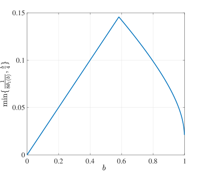
Using Lemma 1 with results in
| (38) |
for arbitrary . Since is decreasing in and is increasing in , the largest value for their minimum is achieved when , i.e., . This is solved for and the achieved maximum value is approximately as shown in Fig. 1
IV Proof of Proposition 2
Since is positive-semidefinite, its eigenvalues are all nonnegative. We begin with the inequality in (32). Assume (10) holds for some such that . Then
| (39) | |||||
for all such that , or equivalently, . Since by assumption, then
| (40) |
for every . Therefore, for every and we can loosen the upper bound in (39) as
| (41) | |||||
At this point, we adopt the notations
| (42) |
for notational simplicity. Let us call the exponent on the right side of (41) by , i.e.,
| (43) |
It is straightforward to check that the function is convex and achieves its minimum over its domain at
| (44) |
It follows that the expression on the right side of (41) achieves its minimum at
| (45) |
We consider two cases:
-
1.
Let , or equivalently,
(46) Then
(47) where we omit the simple algebra.
-
2.
Let . Then
(48)
Let us denote the expression on the right side of (46) by , i.e.,
| (49) |
To recap, we have shown that
| (50) |
and
| (53) |
Next, the next lemma explores a possibility for . It addresses an inequality for which (10) is a special case.
Lemma 2.
Let be an integer. For every , the inequality
| (54) |
holds with
| (55) |
Proof.
See Appendix B. ∎
V Proof of Proposition 3
To see how (13) implies HW inequality, let us write HW inequality in (2) as
| (58) |
Note
| (61) |
We aim to show that there is such that the upper bound in (50) is less than or equal to the upper bound in (58), or equivalently, . We want this to hold regardless of . Thus, we look for largest such that
| (62) |
Interestingly, the ratio depends on only through the ratio
| (63) |
For ease of comparing the right sides in (16) and (61), we fix such that , i.e., . This quadratic equation has only one root in the admissible domain . We denote this value of by given by
| (64) |
One can easily check that the corresponding value for by . Then we have
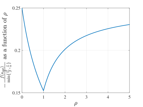
| (67) |
Fig. 2 shows the graph of the function of on the right side of (67). It achieves its absolute minimum value at . It follows that the value for the infimum on the right side of (62) is
| (68) |
It is shown in Appendix C that the choice of in (64) results in the largest value for .
Finally, we address LM inequality itself. Let us write LM inequality in (4) slightly differently as follows. Call where are as in (42). Solving for , we get . Relabeling as , LM inequality becomes
| (69) |
Consider HW inequality in (58). LM inequality implies HW inequality for all satisfying
| (70) |
Once again, we realize that the ratio on the right side of (70) depends entirely on the ratio . It is given by
| (73) |
One can easily check that this function of achieves it absolute minimum value of at . This establishes Proposition 3.
VI Proof of Proposition 4
We begin with the bound in (32). By Lemma 1 in Section III, for every integer and , the inequality in (19) is the tightest for . Then
| (74) | |||||
for all such that , or equivalently, . The value of that minimizes the right side of (74) in terms of is not tractable for arbitrary integer . Instead, let be the value of such that the sum of the first two terms in the exponent, i.e., is minimized. It is given by
| (75) |
We plug in on the right side in (74) where333
| (76) |
The third term in the exponent in (74) is bounded by
| (77) | |||||
where the last step is due to . Next, we bound the sum of the first two terms, namely, . We consider two cases:
-
1.
Let . Then and simple algebra shows that
(78) where
(79) -
2.
Let . Then and we have
(80) where
(81)
| (82) | |||||
VII Proof of Proposition 5
Consider the bound in (74) for , i.e.,
| (83) |
where is given by
| (84) |
and and are defined in (22). The function achieves it global minimum value over at given by
| (85) |
It follows that the minimum value for over the interval is achieved at
| (86) |
Two cases are considered:
-
1.
Let . Then and . To continue, we need the following lemma.
Lemma 3.
Let be positive numbers such that and . Then
(87) Proof.
See Appendix D. ∎
Applying Lemma 3 with , , and and noting that due to , we obtain
(88) -
2.
Let . Then and
(89) Next, we bound the two terms on the right side of (89). We write the second term as
(90) where the penultimate step uses the fact that is a decreasing function in terms of and . Alternatively, we can bound as
(91) where we simply use the fact that as . Using the tighter bound in (90) and (91), we get
(92) Regarding the third term on the right side of (89), note that where we used the trivial inequality for . Then
(93) (94)
Appendix A; Proof of Lemma 1
Define the function by
| (95) |
We study the cases and , separately.
-
•
Let . Then and we get
(96) The only positive first-order critical number for is . If , one easily checks that over an open interval around . Since , then the Mean Value Theorem (MVT) implies that over and hence, (6) can not hold for any . Conversely, let . Then , over and over . Note that . This tells us that rises about on right of , reaches an absolute maximum value at the critical number and then goes down from there on and escapes to on left of . As such, possesses a unique zero (x-crossing) somewhere over . We let be this zero. Then (6) clearly holds for . Finally, we show that is , or equivalently, . We have , i.e.,
(97) Recalling the Maclaurin series for , we have . Then (97) can be simplified as
(98) and hence,
(99) Changing the index to , we get , i.e., as promised.
-
•
Now, let . If is odd, is given by as in the previous case and one easily checks that for , given in (96) is negative for every . Then MVT implies that for every as desired. If is even, then . A similar computation as in (96) gives that
(100) Since is even, once again we have for every and MVT comes in one last time to confirm that for .
VIII Appendix B; Proof of Lemma 2
Assume is an integer and fix . Define the function by
(101) One can easily check that
(102) The only positive first-order critical number for over the interval is given by . Moreover, for and for . Since , then MVT implies that for all in the interval and hence, (10) holds with .
Appendix C; The choice of in (16) results in the largest
In order to compare in (53) with , we address the cases and separately.
-
1.
Let , or equivalently, . Then
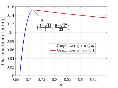
(106) One can easily check that this is a continuous function of and it achieves its absolute minimum value of at .
-
2.
Let , or equivalently, . Then
(110) It is routine to check that this is a continuous function of and it achieves its absolute minimum value of at .
We have shown that
| (113) |
We need to choose such that the right side of (113) is as large as possible. Fig. LABEL:pic_1111 shows the graph of this function over the interval . We see that it achieves its absolute maximum value of at .
Appendix D; Proof of Lemma 3
Define the function
| (114) |
Tedious algebra shows that
| (115) |
We show that is decreasing in for given . Another round of tedious algebra shows
| (116) |
Then follows by noting that for all .
References
- [1] D. L. Hanson and F. T. Wright, “A bound on tail probabilities for quadratic forms in independent random variables”, The Annals of Math. Statistics, vol. 42, no. 3, pp. 1079-1083, 1971.
- [2] M. Rudelson and R. Vershynin, “Hanson-Wright inequality and sub-gaussian concentration”, Electronic Commun. in Probability, vol. 18, no. 82, pp. 1-9, 2013.
- [3] C. Giraud, “Introduction to high-dimensional statistics”, CRC Press, 2nd Edition, 2022.
- [4] E. Giné and R. Nickl, “Mathematical foundations of infinite-dimensional statistical models", Cambridge University Press, 2016.
- [5] B. Laurent and P. Massart, “Adaptive estimation of a quadratic functional by model selection", The Annals of Statistics, vol. 28, no. 5, pp. 1302-1338, 2000.