Learning Networks from Wide-Sense Stationary Stochastic Processes

Abstract

Complex networked systems driven by latent inputs are common in fields like neuroscience, finance, and engineering. A key inference problem here is to learn edge connectivity from node outputs (potentials). We focus on systems governed by steady-state linear conservation laws: $X_{t}={L^{\ast}}Y_{t}$, where $X_{t},Y_{t}\in\mathbb{R}^{p}$ denote inputs and potentials, respectively, and the sparsity pattern of the $p\times p$ Laplacian $L^{\ast}$ encodes the edge structure. Assuming $X_{t}$ to be a wide-sense stationary stochastic process with a known spectral density matrix, we learn the support of $L^{\ast}$ from temporally correlated samples of $Y_{t}$ via an $\ell_{1}$-regularized Whittle’s maximum likelihood estimator (MLE). The regularization is particularly useful for learning large-scale networks in the high-dimensional setting where the network size $p$ significantly exceeds the number of samples $n$.

We show that the MLE problem is strictly convex, admitting a unique solution. Under a novel mutual incoherence condition and certain sufficient conditions on $(n,p,d)$, we show that the ML estimate recovers the sparsity pattern of $L^{\ast}$ with high probability, where $d$ is the maximum degree of the graph underlying $L^{\ast}$. We provide recovery guarantees for $L^{\ast}$ in element-wise maximum, Frobenius, and operator norms. Finally, we complement our theoretical results with several simulation studies on synthetic and benchmark datasets, including engineered systems (power and water networks), and real-world datasets from neural systems (such as the human brain).

Keywords Network topology inference, Conservation laws, $\ell_{1}$-regularized Whittle’s likelihood estimator, Spectral precision matrix.

1 Introduction

Complex networked systems, composed of nodes and edges that connect them are commonly used to model real-world systems in fields such as neuroscience, engineering, climate, and finance [1, 2]. We study networks governed by conservation laws that control edge flows; examples include current in electrical grids, fluids in pipelines, and traffic in transportation systems [3, 4]. In neuroscience, there is growing interest in identifying and understanding conservation laws [5, 6].

Networked systems driven by latent inputs (i.e., nodal injections) generate edge flows that are proportional to differences in node potentials. For example, in electrical networks, nodal current injections induce current flows that are proportional to potential differences between nodes. The overall dynamics of these edge flows are governed by conservation laws. Formally, for a network of size $p$, these dynamics are described by the balance equation $X=L^{\ast}Y$, where $L^{\ast}\in\mathbb{R}^{p\times p}$ is a weighted symmetric Laplacian matrix [7]. The off-diagonal entries of $L^{\ast}$ capture the edge connectivity structure of the network. Vectors $X,Y\in\mathbb{R}^{p}$ represent nodal injections and potentials respectively, and in this paper we treat them as random vectors. Further details on the balance equation are in Section 2.

In various practical situations, the network’s connectivity is typically not known and needs to be estimated for modeling, management, and control tasks. This involves determining the non-zero elements of the associated Laplacian matrix $L^{\ast}$. Previous methods such as [8] estimate $L^{\ast}$ given observations of node injection-potential pairs $\{X,Y\}$ by minimizing an appropriate least squares objective. Such methods critically rely on the ability to observe both injections and potentials simultaneously. However, node injections are often unobservable in various scenarios. For instance, in financial or brain networks, nodal injections correspond to economic shocks or unknown stimuli, and these are not observable by the measurement system in place. In these settings, the goal is to estimate $L^{\ast}$ with only samples of $Y$. Indeed this problem is ill-posed as multiple solutions of $X$ and $L^{\ast}$ can satisfy the equation $X=L^{\ast}Y$. To address the ill-posedness, we assume we have access to some information about the distribution of $X$. The challenge of estimating $L^{\ast}$ from $Y$ under such assumptions have been previously studied in [9, 10, 11].

This line of work relies on the observations of the potentials being independent and identically distributed (i.i.d.). When temporal dependencies exist in the data, such methods are insufficient. In this paper, we adopt a more realistic data model and suppose that the nodal injections ($X_{t}$) and potentials ($Y_{t}$) are wide-sense stationary processes (WSS). This generalization allows for a more flexible framework for network learning while posing some interesting technical challenges. Before we outline our major contributions, we will first state the problem more formally and outline the challenges it presents.

Structure learning problem: Given finite samples of node potentials $\{Y_{t}\}_{t=1}^{n}$ and assuming the node injections $X_{t}$ are generated from a WSS process with known spectral density matrix, the goal is to recover the matrix $L^{\ast}\in\mathbb{R}^{p\times p}$ such that the estimate $\widehat{L}$ approximately satisfies the balance equation $X_{t}\approx\widehat{L}Y_{t}$.

While the structure learning problem can be addressed through a two-step process—first estimating the spectral density of $Y_{t}$ from $\{Y_{t}\}_{t=1}^{n}$, then estimating $L^{\ast}$ from the spectral density of $X_{t}$—this approach is statistically inefficient, even when $Y_{t}$ is i.i.d., this is elaborated in Remark 3 of [9]. To overcome these limitations, we propose a novel single-step estimator for $L^{\ast}$ that integrates time-series data with the constraints imposed by conservation laws. Our method also ensures consistent estimation of $L^{\ast}$ in the high-dimensional setting where the number of samples $n$ is significantly smaller than the network size $p$ (i.e., $n\ll p$). This requires that $L^{\ast}$ is sparse, which is natural in all of our motivating examples; power grids, social networks, and brain connectivity graphs are inherently sparse, with nodes connected to only a small subset of others. We now provide a high-level overview of our methodology.

Suppose that $\{X_{t}\}_{t\in\mathbb{Z}}$ is a WSS process with a power spectral density matrix $f_{X}(\omega)$ with $\omega\in[-\pi,\pi]$ (see (3) for a formal definition). The conservation law forces the spectral density $f_{Y}(\omega)$ of $\{Y_{t}\}_{t\in\mathbb{Z}}$ to satisfy $f_{X}(\omega)=L^{\ast}f_{Y}(\omega)(L^{\ast})^{\mathsf{T}}$. Given samples from the node potential process $\{Y_{t}\}_{t=1}^{n}$ and assuming that $f_{X}(\omega)$ is known (this is all we assume we know about $X$), consider the optimization problem:

$$\underset{L\in\mathbb{R}^{p\times p}}{\text{maximize}} \mathcal{L}[\{Y_{t}\}_{t=1}^{n};f_{X}(\omega)]+\lambda_{n}\|L\|_{1}$$ (1)

subject to $$f_{X}(\omega)=Lf_{Y}(\omega)L^{\mathsf{T}},\quad\omega\in[-\pi,\pi],$$

where $\mathcal{L}[\cdot]$ is an appropriate log-likelihood that measures the fit to observed data, and $\lambda_{n}\geq 0$ is a regularization parameter. The $\ell_{1}$-norm $\|\cdot\|_{1}$ (which is the entry-wise absolute sum) helps promote sparsity in our estimate of $L^{\ast}$. Full details of (1) are in Section 2. While such optimization problems that target sparse matrix estimation have received considerable attention in the literature (see Section 5 and Section 1.2 for an account of this), (1) presents some unique challenges:

1. $\{Y_{t}\}_{t=1}^{n}$ is not i.i.d., making standard sample covariance matrix style analyses inapplicable;

2. it involves a continuum of constraints since $\omega\in[-\pi,\pi]$, rendering (1) an infinite-dimensional optimization problem; and

3. the constraint is non-convex for arbitrary matrices $L$, even when considering the symmetry of the Laplacian matrix.

Although a line of work [12, 13, 14, 15] addresses challenges of the form (i) and (ii) separately in the context of learning Gaussian graphical models from time-series data, and [9] tackles challenge (iii), no prior work, to the best of our knowledge addresses all three challenges simultaneously. The goal of this paper is to show that despite these challenges, the optimizer of (1) captures the sparsity pattern of $L^{\ast}$ with high probability. Thus, the optimizer of (1) is the estimator we seek to recover the sparse matrix $L^{\ast}$. This problem formulation is motivated by several applications where it plays a natural role; here we briefly outline two.

1) Topology learning in power distribution networks: Knowledge of network topology (or structure) enables better fault detection, efficient resource allocation, and better integration of decentralized energy resources, ensuring reliable operation of the power system. However, system operators may lack access to real-time topology information and use nodal voltages or current injections to learn the network topology. A balance equation of the form $X_{t}={L^{\ast}}Y_{t}$, where $L^{\ast}$ is the network admittance matrix and injected currents $X_{t}$ modeled by a WSS process, has been considered in this context [16].

2) Learning sensor to source mapping in the human brain: Learning the mapping from source signals to EEG electrodes is crucial for analyzing brain connections. Many studies [17, 18] suggest a model of the form in (2). Specifically, the Laplacian matrix plays the role of lead-field matrix and the potentials $Y_{t}$ are the EEG signals. The injections $X_{t}$ model the latent source signals and are thought to be generated by a vector auto-regressive process (VAR$(m)$): $X_{t}=\sum_{k=1}^{m}A_{k}x_{t-k}+\epsilon_{t}$, where $\epsilon_{t}$ could be non-Gaussian; and the integer $m$ and matrices $A_{k}$ could be known or unknown. Thus, learning the source mapping involves learning $L^{\ast}$ from WSS data.

1.1 Main contributions

1) A novel convex estimator: We propose an $\ell_{1}$-regularized log-likelihood estimator of the form (1) to estimate $L^{\ast}$ from finite samples of WSS data $\{Y_{t}\}_{t=1}^{n}$. This estimator builds on the Whittle log-likelihood approximation (details in Section 2.2). Our first theoretical result establishes that the proposed $\ell_{1}$-regularized estimator is convex in $L$ and under standard conditions, admits a unique minimum even in the high-dimensional regime ($n\ll p$).

Since the Whittle likelihood is closely tied to the likelihood of Gaussian WSS processes, our estimator maximizes an approximate Gaussian likelihood. However, the estimator remains meaningful even for non-Gaussian injections $\{X_{t}\}_{t\in\mathbb{Z}}$, including stationary linear processes with sub-exponential or finite fourth-moment error distributions (see the remark on Bregman divergence in Section 2.2).

2) Sample complexity and estimation consistency: We provide sufficient conditions on the sample size $n$ of the data $\{Y_{t}\}_{t=1}^{n}$ for the estimator to achieve two key properties: sparsistency, ensuring the recovery of the sparsity pattern of $L^{\ast}$, and norm consistency, providing error bounds in terms of element-wise maximum, Frobenius, and operator norms. Pivotal to our analysis is a novel irrepresentability-like condition on $L^{\ast}$, inspired by similar conditions commonly used in high-dimensional statistics [19, 20]. The sample complexity results are derived for both Gaussian and linear non-Gaussian WSS processes (see Theorem 1 and 2).

3) Experimental validation: We validate our theoretical results with extensive numerical experiments using synthetic and quasi-synthetic data from many benchmark networked systems, as well as a real-world dataset involving the brain network (see Section 4).

1.2 Related work

1.2.1 Structure learning in Gaussian graphical models (GGMs)

The graph underlying a GGM can be inferred from the sparsity pattern of the inverse covariance matrix, and numerous papers have focused on learning this pattern from i.i.d. data (see [21] for an overview). Pioneering works like  [22, 23] have developed key theoretical concepts for analyzing $\ell_{1}$-regularized likelihood estimators, and our analysis builds on these concepts. Other works like  [24, 25] focus on learning Cholesky factors of the inverse covariance matrix, but they lack theoretical guarantees. Survey papers like [26] provide a comprehensive overview of estimators for GGMs in various scenarios, including dynamic and grouped networks, while [27] presents detailed analyses of theoretical frameworks and sample complexity results for these models. However, these approaches face two significant limitations in our context. First, they are primarily designed for i.i.d. data, whereas the problem we address involves time-series data. Second, these methods aim to estimate the inverse covariance matrix, whereas our focus is to estimate the Laplacian $L^{\ast}$ directly, bypassing the need to first estimate the inverse covariance matrix.

1.2.2 Graph signal processing (GSP)

Recent research in GSP studied sparse inverse covariance estimation problems in GGMs by imposing Laplacian constraints. Both the regularized likelihood and spectral template-based (i.e., using eigenvectors of the sample covariance matrix) techniques are used to learn the Laplacian-constrained inverse covariance matrix [28, 29, 30]. However, many papers in this area focus only on estimation consistency or algorithmic convergence, but not on sample complexity. In our problem, the inverse covariance (or spectral density) matrix is represented as a quadratic matrix equation involving products of Laplacian matrices (see (1)), making existing methods in the cited works unsuitable for direct application. In addition, we provide sample complexity guarantees and establish precise rates of convergence for our proposed estimator.

1.2.3 Learning network structure from WSS process

Dahlhaus [31] showed that the sparsity pattern of the inverse spectral density (ISD) matrix represents the structure of the graphical model for a Gaussian WSS. Subsequently, many papers (see e.g., [12, 32]) have focused on estimating a sparse ISD matrix. Finally, a few more (see [13, 14, 15]) have focused on estimating parameter matrices of latent models (e.g., VAR or state-space) generating the ISD matrix. Our research falls into the latter category, with a parameter matrix that is a Laplacian of a conservation law. However, directly applying these methods often leads to a two-stage approach: first estimating the parameter matrix, followed by a refinement step to identify non-zero entries in $L^{\ast}$. In contrast, our estimator of the form in (1) directly estimates the Laplacian matrix $L^{\ast}$, thus avoiding the statistical inefficiencies inherent in the two-stage approach (see Section 1.2.1).

1.2.4 Electric power networks

While there are many motivating examples for the framework considered here, the authors were specifically motivated by the problem of topology learning in power networks. For i.i.d. data, works like [33, 34] infer the sparsity pattern of the Laplacian (associated with a conservation law under linear power flow) by learning the inverse covariance of node potentials and applying algebraic rules. This approach requires minimum cycle length conditions on the network, which we do not need (see Remark 3). Survey papers like [35] provide a good overview of state-of-the-art methods, including the likelihood approaches in [36].

We now contrast this work with a related paper by a subset of the authors [9]. First, the estimator in  [9] assumes i.i.d. Gaussian injections $X_{t}$, whereas the current work addresses non-i.i.d. $X_{t}$ and considers a broader class of Gaussian and non-Gaussian WSS processes; we outlined the unique challenges in the discussion following equation (1). Second, our analysis requires a comprehensive examination of Hermitian matrices in the optimization problem, which is more complex than dealing solely with symmetric matrices, as in [9]. Third, we empirically validate the performance of our estimator, particularly regarding sample complexity and error consistency, across a wide range of networked systems, and compare it directly with the estimator proposed in [9].

Notation: Let $\mathbb{Z},\mathbb{R}$, and $\mathbb{C}$ denote sets of integers, reals, and complex numbers, respectively. For sets $T_{1},T_{2}\subset[p]\times[p]$, denote by $A_{T_{1}T_{2}}$ the submatrix of $A$ with rows and columns indexed by $T_{1}$ and $T_{2}$. If $T_{1}=T_{2}$, we denote the submatrix by $A_{T_{1}}$. For a matrix $A=[A_{i,j}]$, $\|A\|_{F}$ and $\|A\|_{2}$ denote the Frobenius and the operator norm; $\|A\|_{\infty}\triangleq\max_{i,j}|A_{ij}|$ and $\|A\|_{1,\text{off}}=\sum_{i\neq j}|A_{ij}|$. The $\operatorname{\ell_{\infty}}$-matrix norm of $A$ is defined as $\nu_{A}=\left|\kern-1.07639pt\left|\kern-1.07639pt\left|A\right|\kern-1.07639pt\right|\kern-1.07639pt\right|_{\infty}\triangleq\max_{j=1,\ldots,p}\sum_{j=1}^{p}|A_{ij}|.$ We use $\operatorname*{\text{vec}}(A)$ to denote the $p^{2}$-vector formed by stacking the columns of $A$ and $\Gamma(A)=(I\otimes A)$ to denote the Kronecker product of $A$ with the identity matrix $I$. For two symmetric positive definite matrices $A_{1}$ and $A_{2}$, $A_{1}\succ A_{2}$ means $A_{1}-A_{2}$ is positive definite. We define $\text{sign}(A_{ij})=+1$ if $A_{ij}>0$ and $\text{sign}(A_{ij})=-1$ if $A_{ij}<0$. For two-real valued functions $f(\cdot)$ and $g(\cdot)$, we write $f(n)=\mathcal{O}(g(n))$ if $f(n)\leq cg(n)$ and $f(n)=\Omega(g(n))$ if $f(n)\geq c^{\prime}g(n)$ for constants $c,c^{\prime}>0.$

Organization of the paper: In Section 2, we define the structure learning problem and propose the modified $\ell_{1}$-regularized Whittle likelihood estimator for learning a network structure from WSS data. Section 3 establishes the convexity of the proposed estimator and provides guarantees for support recovery and norm consistency for both Gaussian and non-Gaussian node injections $X_{t}$. In Section 4, we evaluate the performance of our estimator on synthetic, benchmark, and real-world datasets. Section 5 emphasizes the parallels that our structure learning framework shares by drawing connections to other learning problems in the literature. Finally, Section 6 concludes with a summary and outlines future directions. Proofs of theoretical results and additional experimental details are provided in the supplementary material. Throughout, we use estimation and learning interchangeably, as well as network and graph.

2 Preliminaries and Problem Setup

For directed graph $\mathcal{G}=([p],E)$, where the node set is defined as $[p]\triangleq\{1,2,\ldots,p\}$ and the edge set is $E\subseteq[p]\times[p]$, let $\mathcal{D}$ denote the $p\times\left|E\right|$ incidence matrix. Each column of $\mathcal{D}$ corresponds to an edge $(i,j)$ and is populated with zeros except at the $i$-th and $j$-th positions, where it takes the values $-1$ and $+1$, respectively. Suppose $X\in\mathbb{R}^{p}$ denotes the vector of node injections. The basic conservation law is given by: $\mathcal{D}f+X=0$, where $f\in\mathbb{R}^{\left|E\right|}$ is the vector of edge flows. This law states that the sum of flows over the edges incident to a vertex equal the injected flow at that vertex. In other words, edge and injected flows are conserved.

In physical systems, edge flows are determined by potentials $Y\in\mathbb{R}^{p}$ at the vertices. Under natural linearity assumptions, the edge flow on the $(i,j)$-th edge is proportional to $Y_{j}-Y_{i}$. For all edges, $f=-\mathcal{D}^{\mathsf{T}}Y$. Substituting this edge flow relation in the basic conservation law yields the balance equation:

$$X-L^{\ast}Y=0,$$ (2)

where $L^{\ast}\triangleq\mathcal{D}\mathcal{D}^{\mathsf{T}}$ is the $p\times p$ real-valued symmetric Laplacian matrix. A typical system satisfying (2) is an electrical network with unit resistances, where $Y$ represents voltage potentials, $f$ edge currents, and $X$ injected currents. For examples involving hydraulic, social, and transportation systems, see [3, 4].

2.1 Structure learning problem

The sparsity pattern (locations of zero and non-zero entries) of $L^{\ast}$ reflects the edge connectivity of the underlying network. Specifically, $(i,j)\in E$ if and only if $L^{\ast}_{ij}\neq 0$. Our goal is to learn the unknown edge set $E$ (or the sparsity pattern of $L^{\ast}$) from data collected at the nodes of the graph.

Let $\{X_{t}\}_{t\in\mathbb{Z}}$ be a zero-mean $p$-dimensional vector-valued WSS process, where, for each $t\in\mathbb{Z}$, $X_{t}=(X_{t1},\ldots,X_{tp})^{\mathsf{T}}\in\mathbb{R}^{p}$. The auto-covariance function of this process is $\Phi_{X}(l)\triangleq\mathbb{E}[X_{t}X_{t-l}^{\mathsf{T}}],\text{ for all }t\in\mathbb{Z}$ and $l\in\mathbb{Z}$ is the lag parameter. We assume that $\Phi_{X}(l)\succ 0$. Because $\{X_{t}\}_{t\in\mathbb{Z}}$ is WSS, it holds that $\|\Phi_{X}(l)\|_{2}<\infty$. Hence, the power spectral density (PSD) function of $\{X_{t}\}_{t\in\mathbb{Z}}$ exists and is defined via the discrete-time Fourier transform of $\Phi_{X}(l)$:

$$f_{X}(\omega) \triangleq\frac{1}{2\pi}\sum_{l=-\infty}^{\infty}\Phi_{X}(l)e^{-\operatorname{i}l\omega},\quad\omega\in[-\pi,\pi],$$ (3)

where $\operatorname{i}=\sqrt{-1}$ and $f_{X}(\omega)\in\mathbb{C}^{p\times p}$ is a Hermitian positive definite matrix. Let $\Theta_{X}(\omega)\!\triangleq\!f_{X}^{-1}(\omega)$ be the inverse PSD.

Let $\{Y_{t}\}_{t\in\mathbb{Z}}$ be generated per the balance equation in (2). We want to obtain a sparse estimate of $L^{\ast}$ using the finite time-series potential data $\{Y_{t}\}_{t=1}^{n}$ and only the nodal injection’s inverse PSD matrix $\Theta_{X}(\omega)$; see Remark 2. We emphasize that our processes need not be Gaussian. A major challenge in developing maximum-likelihood parameter estimates from time-series data is obtaining tractable likelihood formulas. Whittle [37] developed a good approximation for the Gaussian case, and the later work extended this approach to other cases. Following [12], we provide likelihood approximations for $\{Y_{t}\}_{t=1}^{n}$.

2.2 Modified Whittle’s likelihood approximation

Suppose that $L^{\ast}$ is invertible (see Remark 1), the equation in (2) simplifies to $Y_{t}={(L^{\ast})}^{-1}X_{t}$. Due to this linear relationship, $\{Y_{t}\}_{t\in\mathbb{Z}}$ is also a WSS process with the auto-covariance matrix:

$$\Phi_{Y}(l)\triangleq\mathbb{E}[Y_{t},Y_{t-l}^{\mathsf{T}}]={(L^{\ast})}^{-1}\Phi_{X}(l){(L^{\ast})}^{-1},$$

and the PSD matrix:

$$f_{Y}(\omega)\triangleq\frac{1}{2\pi}\sum_{l=-\infty}^{\infty}\Phi_{Y}(l)e^{-\operatorname{i}l\omega}={(L^{\ast})}^{-1}f_{X}(\omega){(L^{\ast})}^{-1},$$ (4)

where $\omega\in[-\pi,\pi]$. Finally, define the inverse PSD matrix:

$$\Theta_{Y}(\omega)\triangleq f^{-1}_{Y}(\omega)={L^{\ast}}\Theta_{X}(\omega){L^{\ast}}.$$ (5)

For now assume that $\{Y_{t}\}_{t\in\mathbb{Z}}$ is a WSS Gaussian process. We will relax this assumption later. Define $\omega_{j}=2\pi j/n$ and denote $\mathcal{F}_{n}=\{\omega_{0},\ldots,\omega_{n-1}\}$ to be the set of Fourier frequencies. The discrete Fourier transform (DFT) of $\{Y_{t}\}_{t=1}^{n}$ is then given by $d_{j}=\frac{1}{\sqrt{n}}\sum_{t=1}^{n}Y_{t}e^{-\operatorname{i}t\omega_{j}}\in\mathbb{C}^{p}$. Observe that DFT is a linear transformation; and hence, $d_{j}$s are complex-valued multivariate Gaussian with the inverse covariance $\Theta_{Y}(\omega_{j})\in\mathbb{C}^{p\times p}$.

The log-likelihood of the finite-time series data $\{Y_{t}\}_{t=1}^{n}$ as per the Whittle approximation [37] is given by

$$\frac{1}{2}\sum_{j\in\mathcal{F}_{n}}\left[\log\det(\Theta_{Y}(\omega_{j}))-\operatorname{Tr}(\Theta_{Y}(\omega_{j})d_{j}d^{\dagger}_{j})\right],$$ (6)

where $\dagger$ is the conjugate transpose and we dropped the constants in the approximation that do not depend on $L^{\ast}$. Expression in (6) resembles the log-likelihood formula for i.i.d. $\{Y_{t}\}_{t=1}^{n}$. Thus, we can view $\hat{f}_{j}\triangleq\hat{f}(\omega_{j})=d_{j}d_{j}^{\dagger}$ as playing the role of sample covariance for the spectral density matrix $f_{Y}(\omega_{j})$.

The log-likelihood in (6) requires modifications to serve as a suitable objective function in $\mathcal{L}[\cdot]$ in (1). First, for $\widehat{L}$ to have better statistical performance, the spectral density estimate $\hat{f}_{j}$, which has a high variance (see [38, Proposition 10.3.2]), needs to be smoothed.

We use the averaged periodogram [38]:

$$P_{j}\triangleq P(\omega_{j})=\frac{1}{2\pi(2m+1)}\sum_{|k|\leq m}d(\omega_{j+k})d^{\dagger}(\omega_{j+k}),$$ (7)

where $\omega_{j}\in\mathcal{F}_{n}$ and $P_{j}\in\mathbb{C}^{p\times p}$. The bandwidth $m$ regulates the bias and variance of $P_{j}$ [38], which in turn impact the estimation consistency results for $L^{\ast}$ in Theorem 1 and 2. For a theoretical discussion on periodograms consult [38].

Second, substituting $P_{j}$ given by (7) in (6) results in an approximate likelihood that is analytically intractable because of the double summation that appears within the $\operatorname{Tr}[\cdot]$ operator. We address this by further approximating the likelihood in (6) as suggested by [12]. The idea here is to consider the likelihood in the neighborhood of a frequency $\omega_{j}$, where $j\in\mathcal{F}_{n}$. Thus, for $j-m\leq l\leq j+m$, a reasonable likelihood near $\omega_{j}$ is

$$\frac{1}{2}\sum_{l=j-m}^{j+m}\left[\log\det(\Theta_{Y}(\omega_{l}))-\operatorname{Tr}(\Theta_{Y}(\omega_{l})d_{l}d^{\dagger}_{l})\right].$$ (8)

This local likelihood could be simplified by assuming $\Theta_{X}(\omega)$ is a smooth function of $\omega\in[-\pi,\pi]$. Thus, $\Theta_{X}(\omega_{l})$ is constant for the frequencies neighboring $\omega_{j}$. This smoothness assumption along with the relationship in (5) implies $\Theta_{Y}(\omega_{j})=\Theta_{Y}(\omega_{l})$, for all $j-m\leq l\leq j+m$. Consequently, (8) simplifies to

$$\frac{(2m+1)}{2}\left[\log\det(\Theta_{Y}(\omega_{j}))-\text{Tr}(\Theta_{Y}(\omega_{j})P_{j})\right],$$ (9)

which we call as the modified Whittle’s approximate likelihood for the Gaussian node potentials $\{Y_{t}\}_{t=1}^{n}$.

The modified (per frequency) likelihood in (9) is valid even if $\{Y_{t}\}_{t=1}^{n}$ is non-Gaussian. This is because as $n\to\infty$, the DFT vectors $d_{j}$ converge to a complex-valued multivariate Gaussian with inverse covariance $\Theta_{Y}(\omega_{j})$, per [38, Propositions 11.7.4 and 11.7.3]. Thus, the likelihood either in (6) or in (9) remains applicable for non-Gaussian $\{Y_{t}\}_{t\in Z}$. However, this standard justification relies on $n$ being large and might not be appropriate for smaller $n$. A more robust theoretical justification can be given using Bregman divergences, which we discuss next.

The Bregman divergence between $p\times p$ Hermitian matrices $A$ and $B$ is $D_{\phi}(A;B)\triangleq\phi(A)-\phi(B)-\langle\nabla\phi(B),A-B\rangle$, where $\phi(\cdot)$ is a differentiable, strictly convex function mapping matrices to reals [23, 39]. The log-det Bregman divergence is a special case for $\phi(\cdot)=\log\det[\cdot]$. Thus for $A\succ 0$ and $B\succ 0$ (either real or complex-valued matrices), we have,

$$D_{\phi}(A;B) =-\log\det(A)+\log\det(B)+\operatorname{Tr}(B^{-1}(A-B)).$$

Let $A=\Theta_{Y}(\omega)$; and $B=\Theta^{\ast}_{Y}(\omega)$ be the true inverse spectral density matrix with $f^{\ast}_{Y}={\Theta_{Y}^{\ast}}^{-1}$. We drop terms that do not depend on $\Theta_{Y}(\omega)$ in $D_{\phi}(A;B)$ and note that $D_{\phi}(A;B)$ is proportional to $-\log|\Theta_{Y}(\omega)|+\operatorname{Tr}(f^{\ast}_{Y}(\omega)\Theta_{Y}(\omega))$. Finally, replacing $f^{\ast}_{Y}(\omega)$ in this expression with the periodogoram estimator $P(\omega)$ gives us the negative of the modified likelihood given in (9).

In view of the foregoing discussion, we see that our modified approximate likelihood function in (9) is a good candidate for the loss function $\mathcal{L}[\cdot]$ in (1) even for non-Gaussian $\{Y_{t}\}_{t\in\mathbb{Z}}$.

Remark 1.

(Inverse of $L^{\ast}$). The invertibility assumption is necessary for identifying $L^{\ast}$ from the time series data $\{Y_{t}\}_{t=1}^{n}$. However, $L^{\ast}$ might not be invertible because it has single or multiple zero eigenvalues. A workaround is to use the reduced-order Laplacian, which is obtained by removing $k$ rows and columns from $L^{\ast}$ (see [40]), or to perturb the diagonal of $L^{\ast}$ with a small positive quantity. In power networks, this perturbation corresponds to adding shunt impedance (self-loops in graph theory) at the nodes. We assume that one of the either approaches are in place and that $L^{\ast}$ is invertible.

3 Convexity and Statistical Guarantees

Using the modified Whittle’s approximate likelihood in (9), we first introduce our $\ell_{1}$-regularized estimator as a convex optimization problem. We then present our main results that theoretically characterize the performance of this estimator when $\{X_{t}\}_{t\in\mathbb{Z}}$ is Gaussian and more generally a linear process. Complete proofs are in Appendix.

The invertibility assumption (see Remark 1) and the diagonal dominance property of $L^{\ast}$ imply that $L^{\ast}$ is a symmetric positive definite matrix. Recall that $f^{-1}(\omega)=\Theta(\omega)$, for $\omega\in[-\pi,\pi]$. Given these conditions and the likelihood formula in (9), the optimization problem in (1) modifies to:

$$\hat{L}_{j} =\underset{L\succ 0}{\operatorname{arg\,min}}\,\,\operatorname{Tr}(\Theta_{Y}(\omega_{j})P_{j})\!-\!\log\det(\Theta_{Y}(\omega_{j}))\!+\!\lambda_{n}\|L\|_{1,\text{off}}$$

$$\quad\,\,\text{subject to}\,\,\,\,\Theta_{Y}(\omega_{j})=L\Theta_{X}(\omega_{j})L^{\mathsf{T}},$$ (10)

where $j=\{0,\ldots,n-1\}$, $\lambda_{n}>0$, and $\|L\|_{1,\text{off}}=\sum_{i\neq j}|L_{ij}|$ is the $\ell_{1}$-norm applied to the off-diagonals of $L\in\mathbb{R}^{p\times p}$. Note that the constraint in (1) is stated in terms of the density matrix $f(\omega)$. But note that the constraint in (3) is in terms of the inverse matrix $f^{-1}(\omega)=\Theta(\omega)$.

For ease of notation, we drop $\omega_{j}$ from $\Theta_{X}(\omega_{j})$ and $\Theta_{Y}(\omega_{j})$ and keep the frequency index $j$ only for the averaged periodogram $P_{j}$ (since it captures the influence of periodograms computed at neighboring frequencies of $j$) and the estimator $\widehat{L}_{j}$. Let $D\in\mathbb{C}^{p\times p}$ be the unique Hermitian positive-definite square root of $\Theta_{X}$ satisfying $D^{2}=\Theta_{X}$. Then substituting $\Theta_{Y}=LD^{2}L^{\mathsf{T}}$ and $L=L^{\mathsf{T}}$ in the cost function of (3), followed by an application of the cyclic property of the trace, results in the following unconstrained estimator:

$$\widehat{L}_{j}=\operatorname*{arg\,min}_{L\succ 0}\,\,\operatorname{Tr}(DLP_{j}LD)\!-\!\log\det(L^{2})\!+\!\lambda_{n}\|L\|_{1,\text{off}}.$$ (11)

We dropped constants that bear no effect on the optimization problem. In summary, for $\omega_{j}\in\mathcal{F}_{n}$, we propose a point-wise estimator $\widehat{L}_{j}$ via (11). Hereafter, we refer to $P_{j}$ and $\widehat{L}_{j}$ as $P$ and $\widehat{L}$, respectively, since our results hold for all $\omega_{j}\in\mathcal{F}_{n}$. Finally, we use $P_{1}=\mathfrak{R}(P)$ and $P_{2}=\mathfrak{I}(P)$ to denote the real and imaginary parts of the periodogram $P$ and $\Psi_{1},\Psi_{2}$ to denote the real and imaginary parts of $D^{2}$ respectively.

The following lemma establishes two crucial properties of (11): (i) the objective function is strictly convex in $L$ and (ii) $\widehat{L}$ is unique. The proof of this lemma is in Appendix A.

Lemma 1.

For any $\lambda_{n}\!>\!0$ and $L\!\succ\!0$, if all the diagonals of the averaged periodogram $P_{ii}>0$, then (i) the $\ell_{1}$-regularized Whittle likelihood estimator in (11) is strictly convex and (ii) $\widehat{L}$ in (11) is the unique minima satisfying the sub-gradient condition $2\Psi_{1}\widehat{L}P_{1}-2\Psi_{2}\widehat{L}P_{2}-2\widehat{L}^{-1}\!+\!\lambda_{n}\widehat{Z}\!=\!0$, where $\widehat{Z}$ belong to the sub-gradient $\partial\|L\|_{1,\text{off}}$ evaluated at $\widehat{L}$.

Establishing strict convexity of the objective function in (11) is non-trivial and crucial to derive sample complexity and estimation consistency results discussed in Section 3.3. Furthermore, this strict convexity enforces the existence of unique minima even in the high-dimensional regime ($n\ll p$), where the Hessian of the objective function is rank deficient. The key ingredient in establishing such minima is the coercivity of the objective function (discussed later). The combination of convexity, coercivity, and separable property of the $\ell_{1}$-regularizer also facilitates the development of efficient coordinate descent algorithms, which we leave for future research.

Remark 2.

(Unknown spectral density $\Theta^{-1}_{X}(\omega)$) Our work assumes that $\Theta^{-1}_{X}$ is known. If not, we can use (11) to estimate the product matrix $L^{\ast}D$ instead of $L^{\ast}$, where $D$ is the unique Hermitian positive definite square root of $\Theta_{X}$. The resulting estimator is still meaningful for recovering network structure if the sparsity patterns of $L^{\ast}$ and $L^{\ast}D$ are approximately equal.

Remark 3.

(Advantage of directly estimating $L^{\ast}$) The estimator in (11) directly estimates $L^{\ast}$ subject to the constraint $\Theta_{Y}=L^{\ast}\Theta_{X}L^{\ast}$. In contrast, prior methods (see for e.g., [34]) learn the network structure by first estimating the ISD matrix $\Theta_{Y}$ corresponding to $\{Y_{t}\}_{t=1}^{n}$ and then perform a post-processing step of applying algebraic rules to recover the support of $L^{\ast}$. Ref. [9] explains in great detail as to why this top-stage procedure is inferior to direct estimation in terms of sample complexity for the i.i.d. setting (see Fig. 1 in Ref. [9]). Mutatis mutandis, the same reasoning applies to our problem setup.

3.1 Statement of main results

This section features two main results. The first one concerns the theoretical characterization of the convex estimator in (11) when $\{X_{t}\}_{t\in\mathbb{Z}}$ is a Gaussian time series. And the second one gives such a characterization when $\{X_{t}\}_{t\in\mathbb{Z}}$ is a non-Gaussian linear process. At a high level our result for the Gaussian setting states that as long as the time domain samples $n$ scales as $\Omega(d^{3}\log p)$, the estimate $\widehat{L}$ correctly recovers the true support and is close to $L^{\ast}$ (measured in Frobenius and operator norms) with high probability. Here $d$ is the maximum degree of the graph underlying $L^{\ast}$. In the linear process setting, such a performance is guaranteed if $n$ scales as $\Omega(d^{3}(\log p)^{4+\rho})$ for sub-exponential families with parameter $\rho$ and $\Omega(d^{3}p^{2})$ for distributions with finite fourth moment, respectively.

Our main results rely on three assumptions. These type of assumptions, but not identical, appeared in the literature of $\ell_{1}$-constrained least squares problem [19, 41] and in the literature of $\ell_{1}$-regularized inverse-covariance and spectral density estimation [23, 12]. Define the edge set $\mathcal{E}(L^{\ast})=\{(i,j):L^{\ast}_{ij}\neq 0,\text{for all}\hskip 3.01125pti\neq j\}$. Let $E=\{\mathcal{E}(L^{\ast})\cup(1,1)\ldots\cup(p,p)\}$ be the augmented edge set including edges for the diagonal elements of $L^{\ast}$. Let $E^{c}$ be the set complement of $E$.

[A1] Mutual incoherence condition: Let $\Gamma^{\ast}$ be the Hessian of the log-determinant in (11):

$$\Gamma^{\ast}\triangleq\nabla_{L}^{2}\log\det(L)|_{L=L^{\ast}}={L^{\ast}}^{-1}\otimes{L^{\ast}}^{-1}.$$ (12)

We say that $L^{\ast}$ satisfies the mutual incoherence condition if $\left|\kern-1.07639pt\left|\kern-1.07639pt\left|\Gamma^{\ast}_{E^{c}E}{\Gamma^{\ast}_{EE}}^{-1}\right|\kern-1.07639pt\right|\kern-1.07639pt\right|_{\infty}\leq 1-\alpha$, for some $\alpha\in(0,1]$.

The incoherence condition on $L^{\ast}$ controls the influence of irrelevant variables (elements of the Hessian matrix restricted to $E^{c}\times E$ on relevant ones (elements restricted to $E\times E$). The $\alpha$-incoherence assumption, commonly used in the literature, has been validated for various graphs like chain and grid graphs [23]. While $\alpha$-incoherence in [23, 12] is imposed on the inverse covariance or spectral density matrix, we enforce it on $L^{\ast}$. A similar condition has also been explored in [9].

[A2] Bounding temporal dependence: $\{Y_{t}\}_{t\in\mathbb{Z}}$ has short range dependence: $\sum_{l=-\infty}^{\infty}\|\Phi_{Y}(l)\|_{\infty}<\infty$. Thus, the autocorrelation function $\Phi_{Y}(l)$ decreases quickly as the time lag $l$ increases, leading to negligible temporal dependence between samples that are far apart in time.

This mild assumption holds if the nodal injections $\{X_{t}\}_{t\in\mathbb{Z}}$ exhibits short range dependence: $\sum_{l=-\infty}^{\infty}\|\Phi_{X}(l)\|_{\infty}<\infty$. In fact, $\sum_{l=-\infty}^{\infty}\|\Phi_{Y}(l)\|_{\infty}=\sum_{l=-\infty}^{\infty}\|{L^{\ast}}^{-1}\Phi_{X}(l){L^{\ast}}^{-1}\|_{\infty}\leq\nu_{{L^{\ast}}^{-1}}^{2}\sum_{l=-\infty}^{\infty}\|\Phi_{X}(l)\|_{\infty}<\infty$, where $\nu_{{L^{\ast}}^{-1}}$ is the $\operatorname{\ell_{\infty}}$-matrix norm of ${L^{\ast}}^{-1}$. Notice that in real-systems like power networks, injections typically are short range-dependent processes [42].

[A3] Condition number bound on the Hessian: The condition number $\kappa(\Gamma^{\ast})$ of the Hessian matrix in (12) satisfies:

$$\kappa(\Gamma^{\ast})\triangleq\left|\kern-1.07639pt\left|\kern-1.07639pt\left|{\Gamma^{\ast}}\right|\kern-1.07639pt\right|\kern-1.07639pt\right|_{\infty}\left|\kern-1.07639pt\left|\kern-1.07639pt\left|{\Gamma^{\ast}}^{-1}\right|\kern-1.07639pt\right|\kern-1.07639pt\right|_{\infty}\leq\frac{1}{4d\nu_{D^{2}}\|\Theta^{-1}_{Y}\|_{\infty}C_{\alpha}},$$ (13)

where $C_{\alpha}=1+\frac{24}{\alpha}$, $\alpha\in(0,1]$, and $d$ is the maximum degree of the graph underlying $L^{\ast}$. Bounding $\kappa(\Gamma^{\ast})$ to derive estimation consistency results are standard in the high dimensional graphical model literature [43, 44].

3.1.1 Structure learning with Gaussian injections

Let $\{X_{t}\}_{t\in\mathbb{Z}}$ in (2) be a WSS Gaussian process. Consequently, $\{Y_{t}\}_{t\in\mathbb{Z}}$, a linear transformation of $X_{t}$, is also a WSS Gaussian process. Under this assumption, Theorem 1 provides sufficient conditions on the number of samples $n$ of $Y_{t}$ required so that the estimator $\widehat{L}$ in (11) exactly recovers the sparsity structure of $L^{\ast}$ and achieves norm and sign consistency. Here, sign consistency is defined as $\text{sign}(\widehat{L}_{ij})=\text{sign}(L^{\ast}_{ij})$, for all $(i,j)\in E$. We recall that $\nu_{A}=\left|\kern-1.07639pt\left|\kern-1.07639pt\left|A\right|\kern-1.07639pt\right|\kern-1.07639pt\right|_{\infty}\triangleq\max_{j=1,\ldots,p}\sum_{j=1}^{p}|A_{ij}|$.

Define the two model-dependent quantities:

$$\Omega_{n}(\Theta_{Y}^{-1}) =\max_{r\geq 1,s\leq p}\sum_{|l|<n}|l||\Phi_{Y,rs}(l)|$$ (14)

$$L_{n}(\Theta_{Y}^{-1}) =\max_{r\geq 1,s\leq p}\sum_{|l|>n}|\Phi_{Y,rs}(l)|.$$ (15)

These quantities play a crucial role in the norm consistency bounds presented in Theorem 1 and Theorem A.1 (see Remark 4).

Below is an informal version of the main theorem. A formal statement with all numerical and model-dependent constants is in Appendix A. We define $|L^{\ast}_{\min}|\triangleq\min_{(i,j)\in E}|L^{\ast}_{ij}|$ to be the minimum absolute value of the non-zero entries in $L^{\ast}$. We use $x\underset{\smash{\raisebox{2.58334pt}{$\scriptstyle\sim$}\!}}{\succ}y$ to denote $x\geq cy$, the constant $c$ is independent of model parameters and dimensions.

Theorem 1.

Let the injections $\{X_{t}\}_{t=1}^{n}$ be a WSS Gaussian time series. Consider a single Fourier frequency $\omega_{j}\in[-\pi,\pi]$. Suppose that assumptions in [A1-A3] hold. Define $\alpha>0$ and $C_{\alpha}=1+24/\alpha$. Let $\lambda_{n}=96\nu_{D^{2}}\nu_{L^{\ast}}\delta_{\Theta_{Y}^{-1}}(m,n,p)/\alpha$ and the bandwidth parameter $m\underset{\smash{\raisebox{2.58334pt}{$\scriptstyle\sim$}\!}}{\succ}\left|\kern-1.07639pt\left|\kern-1.07639pt\left|\Theta_{Y}^{-1}\right|\kern-1.07639pt\right|\kern-1.07639pt\right|_{\infty}^{2}\zeta^{2}d^{2}\log p$, where $\zeta=\max\{\nu_{{\Gamma^{\ast}}^{-1}}\nu_{{L^{\ast}}^{-1}}\nu_{L^{\ast}}\nu_{D^{2}}C^{2}_{\alpha},\nu^{2}_{{\Gamma^{\ast}}^{-1}}\nu^{3}_{{L^{\ast}}^{-1}}\nu_{L^{\ast}}\nu_{D^{2}}C^{2}_{\alpha}\}$.

If the sample size $n\underset{\smash{\raisebox{2.58334pt}{$\scriptstyle\sim$}\!}}{\succ}\Omega_{n}(\Theta_{Y}^{-1})\zeta md$. Then with probability greater than $1-1/p^{\tau-2}$, for some $\tau>2$, we have

1. $\widehat{L}$ exactly recovers the sparsity structure ie. $\widehat{L}_{E^{c}}=0$.

2. The estimate $\widehat{L}$ which is the solution of (11) satisfies

   $$\|\widehat{L}-L^{\ast}\|_{\infty}\leq 8\nu^{\prime}\delta_{\Theta_{Y}^{-1}}(m,n,p).$$ (16)

3. $\widehat{L}$ satisfies sign consistency if:

   $$|L^{\ast}_{\min}(E)|\geq 8\nu^{\prime}\delta_{\Theta_{Y}^{-1}}(m,n,p),$$ (17)

where, $\nu^{\prime}=\nu_{{\Gamma^{\ast}}^{-1}}\nu_{D^{2}}\nu_{L^{\ast}}C_{\alpha}$ and $\delta_{\Theta_{Y}^{-1}}(m,n,p)\!=\!\sqrt{\frac{\tau\log p}{m}}+\frac{m+\frac{1}{2\pi}}{n}\Omega_{n}(\Theta_{Y}^{-1})+\frac{1}{2\pi}L_{n}(\Theta_{Y}^{-1})$.

Some remarks are in order. Assume that $\zeta$ and $\left|\kern-1.07639pt\left|\kern-1.07639pt\left|\Theta_{Y}^{-1}\right|\kern-1.07639pt\right|\kern-1.07639pt\right|_{\infty}$ are independent of $(n,p,d)$ and that we are in the high-dimensional regime where $\log p/n\rightarrow 0$ as $(n,p)\rightarrow\infty$. Under assumptions in Theorem 1, and when $n=\Omega(d^{3}\log p)$,

with high probability: (a) The support of $\widehat{L}$ is contained within $L^{\ast}$; meaning there are no false negatives. Furthermore, when $(m/n)\Omega_{n}(\Theta_{Y}^{-1})\rightarrow 0$ as $(m,n)\rightarrow\infty$, part (b) asserts that the element-wise $\operatorname{\ell_{\infty}}$-norm, $\|\widehat{L}-L^{\ast}\|_{\infty}$, vanishes asymptotically (see Remark 4 for further discussion on the asymptotic decay of the error norm). Finally, part (c) establishes the sign consistency of $\widehat{L}$. Crucial is the requirement of $|L^{\ast}_{\min}|=\Omega\left(\delta_{\Theta_{Y}^{-1}}(m,n,p)\right)$, which limits the minimum value (in absolute) of the nonzero entries in $L^{\ast}$. This condition parallels the familiar beta-min condition in the LASSO literature (see [19, 23, 12]).

We state a corollary to Theorem 1 that gives error-consistency rates for $\widehat{L}$ in the Frobenius and operator norms. Let $\mathcal{E}(L^{\ast})=\{(i,j):L^{\ast}_{ij}\neq 0,\text{for all}\hskip 3.01125pti\neq j\}$ be the edge set.

Corollary 1.

Let $s=|\mathcal{E}(L^{\ast})|$ be the cardinality of the edge set $\mathcal{E}(L^{\ast})$. Under the hypothesis as in Theorem 1, with probability greater than $1-\frac{1}{p^{\tau-2}}$, the estimator $\widehat{L}$ defined in (11) satisfies

$$\|\widehat{L}\!-\!L^{\ast}\|_{F} \leq 8\nu^{\prime}(\sqrt{s+p})\delta_{\Theta_{Y}^{-1}}(m,n,p)\quad\text{ and }$$

$$\|{\widehat{L}\!-\!L^{\ast}}\|_{2} \leq 8\nu^{\prime}\min\{d,\sqrt{s+p}\}\delta_{\Theta_{Y}^{-1}}(m,n,p),$$

where $\nu^{\prime}$ and $\delta_{\Theta_{Y}^{-1}}(m,n,p)$ are defined in Theorem 1.

Proof sketch:. Both the Frobenius and operator norm bounds follow by applying standard matrix norm inequalities to the $\operatorname{\ell_{\infty}}$ consistency bound in part (b) of Theorem 1. Importantly, $s+p$ is the bound on maximum number of non-zero entries in $L^{\ast}$, where $s$ is the total number of off-diagonal non-zeros in $L^{\ast}$. Complete details are in Appendix A.

3.1.2 Structure learning for non-Gaussian injections

We consider a class of WSS processes $\{X_{t}\}_{t\in\mathbb{Z}}$ that are not necessarily Gaussian. Examples include Vector Auto Regressive (VAR($p$)) and Vector Auto Regressive Moving Average (VARMA ($p,q$)) models with non-Gaussian noise terms. Such models, and many others, belong to the family of linear WSS processes with absolute summable coefficients:

$$X_{t}=\sum_{l=0}^{\infty}A_{l}\epsilon_{t-l},$$ (18)

where $A_{l}\in\mathbb{R}^{p\times p}$ is known and $\epsilon_{t}\in\mathbb{R}^{p}$ is a zero mean i.i.d. process with tails possibly heavier than Gaussian. The absolute summability $\sum_{l=0}^{\infty}|A_{l}(i,j)|<\infty$ ensures stationarity for all $i,j\in\{1,\ldots,p\}$ [45]. We assume that $\epsilon_{kl}$ (for all $k\in[p]$), the $k$-th component of $\epsilon_{l}\in\mathbb{R}^{p}$, is given by one of the distributions below:

[B1] Sub-Gaussian: There exists $\sigma>0$ such that for all $\eta>0$, we have $\mathbb{P}[|\epsilon_{kl}|>\eta]\leq 2\exp(-\frac{\eta^{2}}{2\sigma^{2}})$.

[B2] Generalized sub-exponential with parameter $\rho>0$: There exists constants $a$ and $b$ such that for all $\eta>0$: $\mathbb{P}[|\epsilon_{kl}|>\eta^{\rho}]\leq a\exp(-b\eta)$.

[B3] Distributions with finite $4^{\text{th}}$ moment: There exists a constant $M>0$ such that $\mathbb{E}[\epsilon_{kl}^{4}]\leq M<\infty$.

We need additional notation. Let $n_{k}=\Omega(d^{3}\mathcal{T}_{k})$ represent the family of sample sizes indexed by $k=\{1,2,3\}$, where $\mathcal{T}_{1}=\log p$ correspond to the distribution in [B1], $\mathcal{T}_{2}=(\log p)^{4+4\rho}$ in [B2], and $\mathcal{T}_{3}=p^{2}$ in [B3].

Theorem 2.

Let $X_{t}$ be given by (18) and $Y_{t}={L^{\ast}}^{-1}X_{t}$. Fix $\omega_{j}\in[-\pi,\pi]$. Let $n_{k}=\Omega(d^{3}\mathcal{T}_{k})$, where $k=\{1,2,3\}$. Then for some $\tau>2$, with probability greater than $1-1/p^{\tau-2}$:

1. $\widehat{L}$ exactly recovers the sparsity structure ie. $\widehat{L}_{E^{c}}=0$.

2. The $\operatorname{\ell_{\infty}}$ bound of the error satisfies:

   $$\|\widehat{L}-L^{\ast}\|_{\infty}=\mathcal{O}(\delta_{\Theta_{Y}^{-1}}^{(k)}(n,m,p)).$$ (19)

3. $\widehat{L}$ satisfies sign consistency if:

   $$|L^{\ast}_{\min}(E)|=\Omega(\delta_{\Theta_{Y}^{-1}}^{(k)}(n,m,p)),$$ (20)

where $\delta_{\Theta_{Y}^{-1}}^{(k)}(n,m,p)$ for $k=\{1,2,3\}$ is given by

$$\delta_{\Theta_{Y}^{-1}}^{(1)}(n,m,p) =\left|\kern-1.07639pt\left|\kern-1.07639pt\left|\Theta_{Y}^{-1}\right|\kern-1.07639pt\right|\kern-1.07639pt\right|_{\infty}\frac{(\tau\log p)^{1/2}}{\sqrt{m}}+\bigtriangleup(n,m,\Theta_{Y}^{-1})$$

$$\delta_{\Theta_{Y}^{-1}}^{(2)}(n,m,p) =\left|\kern-1.07639pt\left|\kern-1.07639pt\left|\Theta_{Y}^{-1}\right|\kern-1.07639pt\right|\kern-1.07639pt\right|_{\infty}\frac{(\tau\log p)^{2+2\rho}}{\sqrt{m}}+\bigtriangleup(n,m,\Theta_{Y}^{-1})$$

$$\delta_{\Theta_{Y}^{-1}}^{(3)}(n,m,p) =\left|\kern-1.07639pt\left|\kern-1.07639pt\left|\Theta^{-1}_{Y}\right|\kern-1.07639pt\right|\kern-1.07639pt\right|_{\infty}\frac{p^{1+\tau}}{\sqrt{m}}+\bigtriangleup(n,m,\Theta_{Y}^{-1}),$$

where $\bigtriangleup(n,m,\Theta_{Y}^{-1})=\frac{m+\frac{1}{2\pi}}{n}\Omega_{n}(\Theta_{Y}^{-1})+\frac{1}{2\pi}L_{n}(\Theta_{Y}^{-1})$.

Remark 4.

(Asymptotic decay rate of the error $\|\widehat{L}-L^{\ast}\|_{\infty}$) The model-dependent quantities $\Omega_{n}(\Theta^{-1}_{Y})$ and $L_{n}(\Theta^{-1}_{Y})$, as defined in (14) and (15), are critical for bounding the element-wise $\ell_{\infty}$-norm of the error $\|\widehat{L}-L^{\ast}\|_{\infty}$ in Theorems 1 and 2. We examine conditions under which this error vanishes asymptotically. Specifically, by definition in (15), the quantity $(\sqrt{\log p/m},L_{n}(\Theta^{-1}_{Y}))\rightarrow 0$ as $(m,n)\rightarrow\infty$. Furthermore, if $(m/n)\Omega_{n}(\Theta^{-1}_{Y})\rightarrow 0$ as $(m,n)\rightarrow\infty$, then the error norm vanishes asymptotically. This condition holds in scenarios where the autocovariance function $\Phi_{Y}(l)$ exhibits a geometric decay rate or if $\{Y_{t}\}_{t\in\mathbb{Z}}$ is a VAR(d) process or other stationary processes with strong mixing conditions (see Proposition 3.4 in [46]). As a consequence, the condition $(m/n)\Omega_{n}(\Theta^{-1}_{Y})\rightarrow 0$ as $(m,n)\rightarrow\infty$ holds for a wide range of stationary processes, leading to asymptotic decay of the error norm.

3.2 Outline of technical analysis for main results

We summarize the key techniques used to prove Theorems 1 and 2. Complete details are in Appendix A. We leverage the primal-dual witness (PDW) method—a general technique used to derive statistical guarantees for sparse convex estimators [23, 19]. Before detailing the PDW method, we state differences in our proof approach compared to the cited literature. First, our analysis is in the frequency domain, this accounts for temporal dependencies from WSS process, requiring careful treatment of the Hermitian matrices $P_{j}$ and $D^{2}$ in (11). Second, unlike most literature where the objective function’s dependence on the optimization variable $L$ is linear, our objective function in (11) has a quadratic dependence. This distinction in the frequency domain necessitates stricter control of the Hessian matrix $\Gamma^{\ast}$ via our assumption [A3].

In the PDW method we construct an optimal primal-dual pair $(\widetilde{L},\widetilde{Z})$ that satisfies the zero sub-gradient condition of the problem in (11). (i) The primal $\widetilde{L}$ is constrained to have the correct signed support $E$ of the true Laplacian matrix $L^{\ast}$ and (ii) The dual $\widetilde{Z}$ is the sub-gradient of $\|L\|_{1,\text{off}}$ evaluated at $\widetilde{L}$. If the dual $\widetilde{Z}$ satisfies the strict dual feasibility condition $\|\widetilde{Z}_{E^{c}}\|_{\infty}<1$. Then the dual acts as a witness to certify that $\widetilde{L}=\widehat{L}$ and $\widetilde{L}$ is indeed the unique global optimum.

3.3 The primal-dual construction and supporting lemmata

We construct an optimal primal-dual pair $(\widetilde{L},\widetilde{Z})$. Lemma 2 gives conditions under which this construction succeeds. First, we determine $\widetilde{L}$ by solving the restricted problem:

$$\widetilde{L}\triangleq\operatorname*{arg\,min}_{L\succ 0,L_{E^{c}}=0}\operatorname{Tr}(DLPLD)\!-\!\log\det(L^{2})\!+\!\lambda_{n}\|L\|_{1,\text{off}}.$$ (21)

Notice that $\widetilde{L}\succ 0$ and $\widetilde{L}_{E^{c}}=0$. We choose the dual $\widetilde{Z}\in\|\widetilde{L}\|_{1,\text{off}}$ to satisfy the zero sub-gradient condition of (21) by setting $\lambda_{n}\widetilde{Z}_{ij}\!=\!-2[\Psi_{1}\widetilde{L}P_{1}]_{ij}+2[\Psi_{2}\widetilde{L}P_{2}]_{ij}+2[\widetilde{L}^{-1}]_{ij}$, for all $(i,j)\in E^{c}$, where $P_{1}$ (resp. $\Psi_{1}$) and $P_{2}$ (resp. $\Psi_{1}$) are the real and imaginary parts of $P$ (resp. $D$). Therefore the pair $(\widetilde{L},\widetilde{Z})$ satisfies the zero sub-gradient condition of the restricted problem in (21).

We verify the strict dual feasibility condition: $|\widetilde{Z}_{ij}|<1$, for any $(i,j)\in E^{c}$. We introduce three quantities. First, $W\triangleq P-\Theta^{-1}_{Y}$ quantifies the error between the averaged periodogram $P$ and the true spectral density matrix $\Theta^{-1}_{Y}$. Second, let $\Delta\triangleq\widetilde{L}-L^{\ast}$ be the measure of distortion between $\widetilde{L}$ given by (21) and the true Laplacian matrix $L^{\ast}$. The final quantity $R(\Delta)$ captures higher order terms in the Taylor expansion of the gradient $\nabla\log\det(\widetilde{L})$ centered around $L^{\ast}$. In fact, expand $\nabla\log\det(\widetilde{L})=\widetilde{L}^{-1}={L^{\ast}}^{-1}+{L^{\ast}}^{-1}\Delta{L^{\ast}}^{-1}+{\widetilde{L}^{-1}-{L^{\ast}}^{-1}-{L^{\ast}}^{-1}\Delta{L^{\ast}}^{-1}}$, and then define $\widetilde{L}^{-1}-{L^{\ast}}^{-1}-{L^{\ast}}^{-1}\Delta{L^{\ast}}^{-1}=R(\Delta)$.

The following lemma establishes the sufficient conditions for ensuring strict dual feasibility.

Lemma 2.

(Conditions for strict-dual-feasibility) Let $\lambda_{n}>0$ and $\alpha$ be defined as in [A1]. Suppose that $\max\{2\nu_{D^{2}}(d\|\Delta\|_{\infty}+\nu_{L^{\ast}})\|W\|_{\infty},\|R(\Delta)\|_{\infty},2\nu_{D^{2}}d\|\Delta\|_{\infty}\|\Theta^{-1}_{Y}\|_{\infty}\}\leq\frac{\alpha\lambda_{n}}{24}$. Then the dual vector $\widetilde{Z}_{E^{c}}$ satisfies $\|\widetilde{Z}_{E^{c}}\|_{\infty}<1$, and hence, $\widetilde{L}=\widehat{L}$.

Proof sketch: Express the sub-gradient condition in Lemma 1 in a vectorized form as a function of $R(\Delta)$, $W=P-\Theta_{Y}^{-1}$, and $\Theta^{-1}_{Y}$. We decompose the vectorized sub-gradient condition into two linear equations corresponding to the edge set $E$ and it’s compliment $E^{c}$. An expression for $\widetilde{Z}_{E^{c}}$ is obtained as a function of $R(\Delta),W$ and $\Theta_{Y}^{-1}$. We finish the proof by utilizing the mutual incoherence condition stated in [A1].

The following results provides us with dimension and model complexity dependent bounds on the remainder term $R(\Delta)$. The proof, adapted from [23, lemma 5], relies on matrix expansion techniques; see Appendix A for details.

Lemma 3.

Suppose that the $\ell_{\infty}$-norm $\|\Delta\|_{\infty}\leq{1}/{(3\nu_{{L^{\ast}}^{-1}}d)}$, then $\|R(\Delta)\|_{\infty}\leq\frac{3}{2}d\|\Delta\|_{\infty}^{2}\nu_{{L^{\ast}}^{-1}}^{3}$.

The result below provides a sufficient condition under which $\operatorname{\ell_{\infty}}$-bound on $\Delta$ in Lemma 3 holds. Full proof in Appendix A.

Lemma 4.

Define $r\!\triangleq\!8\nu_{{\Gamma^{\ast}}^{-1}}[\nu_{D^{2}}\nu_{L^{\ast}}\|W\|_{\infty}\!+\!\lambda_{n}/4]$ and suppose $r\leq\min\{{1}/{(3\nu_{{L^{\ast}}^{-1}}d)},{1}/{(6\nu_{{\Gamma^{\ast}}^{-1}}\nu_{{L^{\ast}}^{-1}}^{3}d)}\}$. Then we have the element-wise $\ell_{\infty}$-bound: $\|\Delta\|_{\infty}=\|\widetilde{L}-L^{\ast}\|_{\infty}\leq r$.

Proof sketch: Since $\widetilde{L}_{E^{c}}=L^{\ast}_{E^{c}}=0$, we note $\|\Delta\|_{\infty}=\|\Delta_{E}\|_{\infty}$, where $\Delta_{E}=\widetilde{L}_{E}-L^{\ast}_{E}$ and it is the solution of the sub-gradient associated with the restricted problem in (21). We construct a continuous function $F:\mathbb{R}^{|E|}\rightarrow\mathbb{R}^{|E|}$ with two properties: (i) it has a unique fixed point $\Delta_{E}$ and (ii) On invoking assumption [A3], $F$ is a contraction—specifically, $F(\mathbb{B}_{r})\subseteq\mathbb{B}_{r}$, where $\mathcal{B}_{r}=\{A\in\mathbb{R^{|E|}}:\|A\|_{\infty}\leq r\}$ and $r$. The proof follows by invoking Brower’s fixed point theorem [47] and exploiting the unique fixed point property of $F$ to show that $\Delta_{E}\in\mathcal{B}_{r}$, and hence, $\|\Delta\|_{\infty}\leq r$.

Remark 5.

A consequence of assumption [A3] is the lower bound on the norm of the Hessian $\left|\kern-1.07639pt\left|\kern-1.07639pt\left|\Gamma^{\ast}\right|\kern-1.07639pt\right|\kern-1.07639pt\right|_{\infty}$. This implies that the curvature at the true minimum $L^{\ast}$ is lower bounded. This bound on the curvature is specific to our problem and helps in attaining a control on the distortion parameter $\Delta$, as demonstrated in Lemma 4.

4 Simulations

We report the results of multiple simulations to validate our theoretical claims. The results in Theorems 1 and 2 involve several constants, along with the dimensional parameters $(n,m,d,p)$. Therefore, we do not expect the theoretical results to capture the nuanced behavior of the simulations in every detail. However, we observe that the learning performance of the estimator in (11) improves as the rescaled sample size $n/({d^{3}\log(p)})$ increases, and that the error norm decreases with increasing $n/\log p$. Additionally, the experimental results are also influenced by the choice of the regularization $\lambda_{n}$. We ran the experiments using CVXPY 1.2, an open-source Python package. The reproducible code for generating simulation results in this paper is publicly available at https://tinyurl.com/LNSWSSP.

4.1 Setup and accuracy evaluation metrics

Our experiments assess the finite-sample performance of the proposed estimator for two families of stochastic injections $\{X_{t}\}_{t\in\mathbb{Z}}$, namely, vector autoregressive (VAR (1)) and vector autoregressive moving average (VARMA (2,2)) processes. These processes not only satisfy our technical assumptions but are also widely used for empirical studies.

(i) VAR(1) process: Here the injections $\{X_{t}\}_{t\in\mathbb{Z}}$ satisfy $X_{t}=AX_{t-1}+\epsilon_{t}$ where $\epsilon_{t}\overset{\text{i.i.d.}}{\sim}\mathcal{N}(0,1)$ and $A=0.7I_{p}$. The PSD matrix of this process, for $z=e^{-i\omega}$ and $\omega\in[-\pi,\pi]$, is

$$f_{X}(\omega)=\frac{1}{2\pi}\left(I_{p}-Az\right)\left(I_{p}-Az^{-1}\right)^{-1}.$$

(ii) VARMA(2,2) process: We let $X_{t}=A_{1}X_{t-1}+A_{2}X_{t-2}+\epsilon_{t}+B_{1}\epsilon_{t-1}+B_{2}\epsilon_{t-2}$ where $\epsilon_{t}\overset{\text{i.i.d.}}{\sim}\mathcal{N}(0,1)$. The PSD matrix of this process, for $z=e^{-i\omega}$ and with $\omega\in[-\pi,\pi]$, is [38]

$$f_{X}(\omega)=\frac{1}{2\pi}\mathcal{A}(z)\mathcal{B}(z)\mathcal{B}^{\dagger}(z)(\mathcal{A}^{-1}(z^{-1}))^{\dagger},$$ (22)

where $\mathcal{A}(z)=I_{p}-\sum_{t=1}^{2}A_{t}z^{t}$ and $\mathcal{B}(z)=I_{p}-\sum_{t=1}^{2}B_{t}z^{t}$. We set $A_{1}=0.4I_{p}$ and $A_{2}=0.2I_{p}$. Furthermore, $B_{1}=1.5(I_{5}+J_{5})$ and $B_{2}=0.75(I_{5}+J_{5})$, where $J_{k}\in\mathbb{R}^{k\times k}$ is the matrix of all ones.

For the above processes, we assume that the nodal observation data $\{Y_{t}\}_{t\in\mathbb{Z}}$ satisfy $Y_{t}={L^{\ast}}^{-1}X_{t}$, where we consider $L^{\ast}$ for synthetic, benchmark, and real-world networks (discussed later). The periodogram of $\{Y_{t}\}_{t=1}^{n}$ at frequency $\omega_{j}$ is then computed as $P(\omega_{j})=\frac{1}{2\pi(2m+1)}\sum_{|k|\leq m}d(\omega_{j+k})d(\omega_{j+k})^{\dagger}$. For simplicity, we set the centering frequency as $\omega_{j}=0$. However, our numerical and theoretical analysis applies to any non-zero Fourier frequency. Further, the bandwidth parameter $m=\sqrt{n}$, which is theoretically justified because we consider the regime $m/n\to 0$ as $(m,n)\to\infty$ where the periodogram is asymptotically unbiased (see Remark 4 and [46]).

We consider sparsistency (the ability to recover the correct edge structure) and norm-consistency (the Frobenius norm of the deviation between $\widehat{L}$ and $L^{\ast}$) metrics to evaluate the estimation performance. We assess sparsistency via the F-score: $\text{F-score}={2\text{TP}}/({2\text{TP}+\text{FP}+\text{FN})}\in[0,1]$, where TP (true positives) is the number of correctly detected edges, FP (false positives) is the number of non-existent edges detected, and FN (false negatives) is the number of actual edges not detected. The higher the F-score the better the estimator’s performance in learning the true structure, with $\text{F-score}=1$ signifying perfect structure recovery.

4.2 Synthetic networks

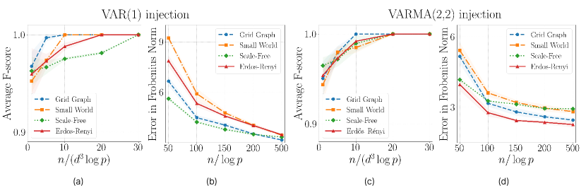
Figure 1: We evaluate the support recovery metric (F-score) and the Frobenius norm error for synthetic random networks under VAR(1) and VARMA(2,2) stochastic injections. Synthetic networks of size $p=30$ are examined, with results averaged over 50 independent trials. Solid curves represent mean performance, while shaded regions around each curve indicate one-sigma standard deviations. The random networks analyzed include grid, small-world, scale-free, and Erdős-Rényi, with maximum degrees $d=\{4,3,9,4\}$, respectively. Panels (a,b) present the average F-score and Frobenius norm error versus rescaled sample size for VAR(1) injection, while panels (c,d) display the same metrics for VARMA(2,2) injection. The rescaled sample size for the F-score is $n/(d^{3}\log p)$, and for the Frobenius norm error, it is $n/\log p$, based on asymptotic convergence rates in Theorem 1. Notably, rescaling the sample size to $n/(d^{3}\log p)$ aligns all curves on top of each other as predicted by Theorem 1.

We present simulations evaluating the performance of the proposed estimator on synthetic random networks. All synthetic networks have a fixed size of $p=30$. The random networks examined in Figure 1 include Erdős-Rényi, Small-World (Watts-Strogatz model), and Scale-Free (Barabási-Albert model) networks, with maximum degrees $d=\{4,3,9\}$, respectively. Additionally, a synthetic grid graph ($d=4$) is constructed by connecting each node to its fourth-nearest neighbor.

For details on constructing synthetic random networks, we refer the readers to [48] and the GitHub repository. In Figure 1 we plot the average F-score and the average Frobenius norm of the error (averaged over 50 independent trials) versus rescaled sample size under VAR(1) and VARMA(2,2) injections. Panels (a-b) depict these metrics for VAR(1) injection, while panels (c-d) show results for VARMA(2,2). The rescaled sample size is $n/(d^{3}\log p)$ for F-score and $n/{\log p}$ for Frobenius norm error—based on asymptotic convergence rates in Theorem 1. As shown in panels (a) and (c), the F-score increases with $n/(d^{3}\log p)$, achieving perfect structure recovery, as predicted by Theorem 1. This causes all plots in panels (a) and (c) to align on top of each other. Panels (b) and (d) demonstrate similar behavior for the Frobenius norm error metric, where the error norm decreases with increase in $n/\log p$.

In Figure 2, we compare F-scores for i.i.d., VAR(1), and VARMA(2,2) injections on an Erdős-Rényi network with size $p=30$ and maximum degree $d=4$. The results indicate that fewer samples are needed to achieve perfect structure recovery (that is, $\text{F-score}=1$) with i.i.d. injections compared to injections of VAR (1) and VARMA (2,2). This trend aligns with theoretical expectations: structure recovery under i.i.d. injections requires $n=\mathcal{O}(d^{2}\log p)$ samples (see [9]), compared to the higher sample complexity of $n=\mathcal{O}(d^{3}\log p)$ for VAR(1) and VARMA(2,2) (see Theorem 1).

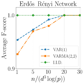
Figure 2: Average F-score comparison for $\{X_{t}\}_{t\in\mathbb{Z}}$ governed by i.i.d., VAR(1), and VARMA(2,2) processes versus rescaled sample size for an Erdős-Rényi network ($p=30$, $d=4$). Perfect structure recovery under VAR(1) and VARMA(2,2) injections requires more samples than under i.i.d. injections.

Finally, we comment on obtaining the regularization parameter $\lambda_{n}$ for experiments in Figure 1 and 2. We apply the extended Bayesian information criterion (EBIC) [49] to select $\lambda_{n}$,

The EBIC is given by:

$$\text{EBIC}_{\gamma}(\widehat{L})=-2\mathcal{L}_{n}(\widehat{L})+|\widehat{E}|\log n+4\gamma|\widehat{E}|\log p,$$ (23)

where $\mathcal{L}_{n}(\widehat{L})$ is the log-likelihood in (11), $\widehat{E}=E(\widehat{L})$ represents the edge set of the candidate graph $\widehat{L}$, and $\gamma\in[0,1]$ is a tuning parameter that influences the penalization. Higher values of $\gamma$ lead to sparser networks. The optimal regularization parameter is $\lambda_{n}=\operatorname*{arg\,min}_{\lambda>0}\text{EBIC}_{\gamma}(\widehat{L})$.

The results in Figure 1 and Figure 2 are for $\gamma=0.4$. In Figure 3, we fix a sample size $n=1000$ and plot the regularization path for both the F-score and Frobenius norm error across various network types. Notably, we observe that for a class of random networks, and the fixed sample size $n=1000$ the value $\log(\lambda_{n})\approx-2$ simultaneously maximizes both the F-score and minimizes the Frobenius norm error.

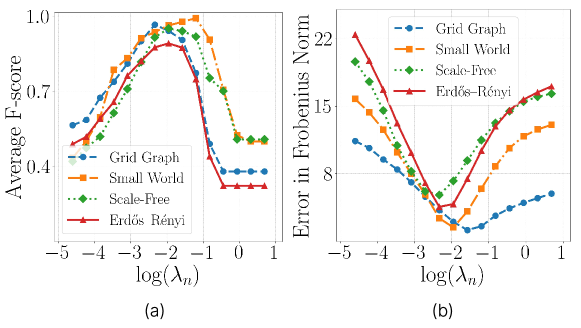
Figure 3: For a fixed sample size $n=1000$, we plot (a) Regularization path for F-score and (b) regularization path for Frobenius norm error, both on a linear-log scale. All networks have $p=30$ nodes, with maximum degrees as follows: grid ($d=4$), small-world ($d=3$), scale-free ($d=9$), and Erdős–Rényi ($d=4$).

4.3 Benchmark networks

For $\{X_{t}\}_{t\in\mathbb{Z}}$ governed by the VARMA(2,2) process, we evaluate the performance of our estimator on three benchmark networks: the power distribution network, water network, and the brain network. Each network has an associated ground truth matrix $L^{\ast}=A+\epsilon I_{p}$, where $A$ is the adjacency matrix that defines the edge structure of the network, $\epsilon=\{2,2,3\}$ for the power, water, and brain networks, respectively, and $I_{p}$ is the $p$-dimensional identity matrix.

1) Power distribution network: We consider the IEEE 33-bus power distribution network whose raw data files are publicly available. An adjacency matrix $A$ can be constructed from this dataset. The network corresponding to $A$ consists of 33 buses and 32 branches (edges) with maximum degree $d=3$.

2) Water distribution network: We examine the Bellingham water distribution network, using data sourced from the database described in [50]. The raw data files are publicly accessible. The ground truth adjacency matrix $A$, containing 121 nodes and 162 edges with maximum degree $d=6$, is generated by loading the raw data files into the WNTR simulator. Complete details on obtaining the adjacency matrix are provided in [51].

3) Brain network: The ground truth adjacency matrix $A$ for this study is publicly accessible, with the detailed methodology regarding its construction described in [52]. The matrix $A$ is a $90\times 90$ matrix (ie. $90$ nodes), where each row and column corresponds to a specific region of interest (ROI) in the brain, as defined by the Automated Anatomical Labeling (AAL) atlas. From 88 patient-derived connectivity matrices found in the database, one was selected (filename: S001.csv) for numerical analyses. The selected network consists of $90$ nodes, $141$ edges and maximum degree $d=7$.

Figure 4 shows the F-score and element-wise $\ell_{\infty}$-norm of the error versus the rescaled sample size. For benchmark networks with varying sizes $p$ and maximum degrees $d$, there is a sharp increase in the F-score when the sample size is $n/(d^{3}\log p)\approx 1$, thus validating the sample complexity of $n=\mathcal{O}(d^{3}\log p)$ as suggested by Theorem 1. This sharp increase in F-score is consistent across different benchmark networks with differing size $p$ and maximum degree $d$. Similarly, across the benchmark networks the element-wise $\ell_{\infty}$-norm of the error decreases sharply at $n/(\log p)\approx 1$.

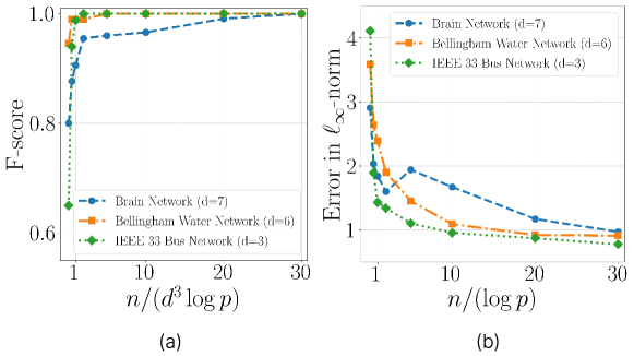
Figure 4: (a) F-score versus rescaled sample size $(n/({d^{3}\log p}))$ across different benchmark networks. (b) Element-wise $\ell_{\infty}$-norm of the error versus rescaled sample size $(n/\log p)$ for the same networks. Both panels compare the human brain structural connectivity network (size $p=90$), Bellingham water network ($p=120$), and IEEE 33 bus power distribution network ($p=33$).

4.4 Real world brain network

We aim to estimate the brain networks for the control and autism groups using fMRI data (obtained under resting-state conditions) from the Autism Brain Imaging Data Exchange (ABIDE) dataset. The pre-processed dataset is accessible, we refer to [53] for more details. For each subject, we have access to $249$ samples of time series measurements across 90 anatomical regions of interest (ROIs) that result in a data matrix, $\{Y_{t}\}_{t=1}^{249}\in\mathbb{R}^{90}$. We collect such measurements for 86 subjects (46 from the autism group and 40 from the control group), from https://github.com/jitkomut/cvxsem.

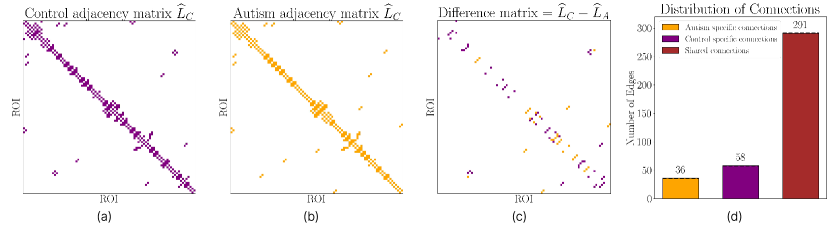
Figure 5: The results here are obtained using a fixed regularization parameter of $\lambda_{n}=0.23$. Each dot in the heatmaps represents a statistically significant edge, i.e., an edge present in more than $90\%$ of the subjects. Panels (a) and (b) display the heatmaps of the estimated common adjacency matrices for the control group ($\widehat{L}_{C}$) and autism group ($\widehat{L}_{A}$), respectively, while panel (c) illustrates the difference matrix, $\widehat{L}_{C}-\widehat{L}_{A}$. This difference matrix captures both control-specific and autism-specific connections. Panel (d) provides a bar plot representing the distribution of connections, detailing the number of group-specific and shared connections. The bar plot indicates that the control adjacency matrix is denser than that of the autism group.

Using this dataset, we estimate a common brain network for each group: one for the control group (among $40$ subjects) and one for the autism group (among $46$ subjects). The common networks are constructed by identifying the statistically significant edges (to be defined later) present across subjects in each group. While our goal is to evaluate the common brain network estimates against the ground truth using metrics like the F-score and Frobenius norm, this is not possible since the true network $L^{\ast}$ is unknown for both groups. Instead, we analyze the relative similarities and differences between the estimated common networks for the control and autism groups.

We begin the experiment by modeling the autocovariance matrix of the noise $\{X_{t}\}$ as $\Phi_{X}(l)=\rho^{|l|}I_{p}$ with $\rho=0.1$, $l=\{1,\ldots,248\}$ and $I_{p}$ is the p-dimensional identity matrix. The noise $\{X_{t}\}$ is therefore a WSS process. The PSD matrix $f_{X}(\omega)=D^{2}$ is computed as the Fourier transform of the autocovariance function $\Phi_{X}(l)$ at $\omega=0$. Our estimator is then applied with regularization $\lambda_{n}=0.23$ across all 86 subjects. The common brain networks for each group are then constructed by retaining the statistically significant edges, that is, the edges that appear in over 90% of the subjects.

Figure 5 (a,b) illustrates the sparsity pattern of the estimated common adjacency matrix for the control group ($\widehat{L}_{C}$) and the autism group ($\widehat{L}_{A}$) brain networks. Each colored point in Figure 5 (a,b) represents a statistically significant edge. We observe that the estimated adjacency matrix for both groups exhibit sparsity as proposed in [54, 55]. In Figure 5 (c), we plot the difference matrix $\widehat{L}_{C}-\widehat{L}_{A}$ to highlight control-specific connections, indicating more connections in the control group than in the autism group. Furthermore, we identify connections that are unique to each group as well as shared across groups. Figure 5 (d) displays a bar plot of the distribution of the group-specific and shared connections, showing that while both groups share numerous connections, the control group exhibits greater connectivity, suggesting a denser network compared to the autism group.

5 Parallels with other structure learning problems

In this section, we loop back to emphasize the generality of the network learning framework considered in this paper. Towards this, we present four examples here that fit well into the framework presented in (1). It is worth noting that many of these assume that $\{Y_{t}\}_{t\in\mathbb{Z}}$ is i.i.d.; so $f_{Y}(\omega)$ is constant. However, we allow for ${\{Y_{t}\}_{t\in\mathbb{Z}}}$ to be a WSS process (which subsumes the i.i.d. case); that is, we do not require $f_{Y}(\omega)$ to be a constant.

1) Graph signal processing (GSP) extends classical signal processing by analyzing signals supported on a graph. For random signals, a simple generative model is $Y_{t}=H(\alpha)X_{t}$. Here $X_{t}$ is white noise and $H(\alpha)=\sum_{k=0}^{K-1}\alpha_{k}S^{k}$ is the graph filter for a given $\alpha_{k}$ and $K$. The shift matrix $S$ (e.g., adjacency or Laplacian) encodes the edge connectivity of the graph. [56] discusses several methods to infer sparsity pattern of $S$ from finitely many observations of $Y_{t}$ for a variety of loss functions $\mathcal{L}[\cdot]$. Note that when $K\to\infty$, $\alpha_{k}=1$, and $S=L-I$, we have $H(\alpha)=(I-S)^{-1}=L^{-1}$. Thus, $f_{Y}(\omega)=H(\alpha)f_{X}(\omega)H(\alpha)^{\mathsf{T}}$ becomes the constraint in our learning problem in (3).

2) Structural equation models (SEMs) are used to model cause-and-effect relationships between variables, allowing us to infer the causal structure of systems in medicine, economics, and social sciences. Networks generated by SEMs, including directed acyclic graphs are of great interest [21].

A random vector $Y_{t}\in\mathbb{R}^{p}$ follows linear SEM if $Y_{t}=B^{\mathsf{T}}Y_{t}+X_{t}$. The path (or autoregressive) matrix $B$ is upper triangular—a structure essential for modeling causal relationships. Therefore we can take $L=I-B^{\mathsf{T}}$ in (3) to reproduce this problem setup. However, our theoretical results need to be suitably adapted to handle a non-symmetric matrix $L$ needed for SEMs, and we leave this for future work.

3) Cholesky decomposition for correlation networks: Let $Y_{t}\sim\mathcal{N}(0,\Sigma)$. The sparsity pattern of $\Sigma$ or the inverse $\Omega=\Sigma^{-1}$ allows us to construct the correlation and partial correlation networks, respectively [57]. Learning sparse covariance or inverse covariance matrices has been well-studied (see Section 1.2).

However, for a clear statistical interpretation, one wants to learn the underlying Cholesky matrices $T$ or $W$, where $\Sigma=TD_{1}T^{\mathsf{T}}$ or $\Omega=WD_{2}W^{\mathsf{T}}$. The sparse triangular matrices $T$ and $W$ can be learned using our framework in (11) by letting $f_{X}(\omega)=D$ and $L^{\ast}=W^{-1}$. However, our approach is more general and does not constrain $L^{\ast}$ to be triangular.

4) Factor analysis (FA) is a statistical method that discovers latent structures within high-dimensional data and is used in Finance and Psychology. The fundamental FA equation is $\tilde{X}_{t}=\Lambda Y_{t}+\Phi U_{t}$. Here $Y_{t}$ and $U_{t}$ are called the common and unique factors; and $\Lambda$ (loading) and $\Phi$ (diagonal) are parametric matrices [58, Chapter 5]. Assuming the contribution from the unique factor is known, define $X_{t}\triangleq\tilde{X}_{t}-\Phi U_{t}=\Lambda Y_{t}$, where $\Lambda$ plays the role of $L^{\ast}$. Then by treating $\tilde{X}_{t}$ as a latent random signal, we can use the estimator in (3) to learn $\Lambda$.

6 Conclusion and Future Work

We study the structure learning problem in systems obeying conservation laws under wide-sense stationary (WSS) stochastic injections. This problem appears in domains like power, the human brain, financial and social networks. We propose a novel $\ell_{1}$-regularized (approximate) Whittle likelihood estimator to solve the network learning problem for WSS injections that include Gaussian and a few classes of non-Gaussian processes. Our theoretical analysis demonstrates that the estimator is convex and has a unique minimum in the high-dimensional setting. We establish sample complexity guarantees for recovering the sparsity structure of $L^{\ast}$, along with norm-consistency bounds (that is, estimation error computed using element-wise maximum, Frobenius, and operator norms). We validate our theoretical results on synthetic, benchmark, and real-world networks under VAR(1) and VARMA(2,2) injections.

We identify three significant future extensions. First, deriving minimax lower bounds to establish the statistical optimality of our estimator building upon the tools developed in [59]. Second, the work in [60] showed that incorporating diagonal dominance and non-positive off-diagonal constraints of Laplacian matrices could improve the estimation performance for precision matrices modeled as Laplacians. Thus, it would be interesting to exploit such constraints into the estimator in (3), and also to relax the symmetry assumption. Non-symmetric Laplacian matrices model directional flows and appear in many fields like transportation, hydrodynamics, and neuronal networks; see [3].

Finally, we could broaden the class of distributions considered for the nodal injection process $X_{t}$. Although we model $X_{t}$ as a WSS process, non-stationarity often arises in applications such as task-based fMRI signals in neuroscience [61] and stock market data, which is frequently modeled by Brownian or Lévy processes [62, 63]. Characterizing sample complexity results for non-stationary processes is challenging and much work needs to be done.

Learning Network Structures from Wide-Sense Stationary Processes: Supplemental Material
Anirudh Rayas, Jiajun Cheng, Rajasekhar Anguluri, Deepjyoti Deka, and Gautam Dasarathy

We restate all theorems, lemmas, and corollaries with their original numbering consistent with the main text. For any new numbered environments introduced exclusively in the appendix, we prefix the labels with "A" (e.g., Lemma A.1). We use $\det(A)$ or $|A|$ to denote the determinant of matrix $A$.

A Proofs of all technical results

After giving a brief overview of the problem set-up and the necessary assumptions, we provide proof for all the technical results. Recall that our observation model is $Y_{t}={L^{\ast}}^{-1}X_{t}$, where $L^{\ast}$ is a $p\times p$ Laplacian matrix (which encodes network structure, that is, $L^{\ast}_{ij}=0$ for all $(i,j)\in E^{c}$); $X_{t}\in\mathbb{R}^{p}$ is a wide sense stationary stochastic (WSS) process with a spectral density matrix $f_{X}(\omega_{j})$ and $Y_{t}\in\mathbb{R}^{p}$ is a random vector of node potentials. Given $n$ samples of $\{Y_{t}\}_{t\in\mathbb{Z}}$ our goal is to learn the sparsity structure of the matrix $L^{\ast}$. We propose the following $\ell_{1}$-regularized Whittle likelihood estimator $\widehat{L}_{j}$ to obtain a sparse estimate of $L^{\ast}$:

$$\widehat{L}_{j}=\operatorname*{arg\,min}_{L\succ 0}\,\,\operatorname{Tr}(DLP_{j}LD)\!-\!\log|L^{2}|\!+\!\lambda_{n}\|L\|_{1,\text{off}},$$ (A.1)

where $D\in\mathbb{R}^{p\times p}$ is the unique Hermitian positive definite square root matrix of $\Theta_{X}$, and $P_{j}=P(\omega_{j})$ is the averaged periodogram. Hereafter, we refer to $P_{j}$ and $\widehat{L}_{j}$ as $P$ and $\widehat{L}$, respectively, since our results hold for all $\omega_{j}\in\mathcal{F}_{n}$. We recall the assumptions to prove our results.

[A1] Mutual incoherence condition: Let $\Gamma^{\ast}$ be the Hessian of the log-determinant in (A.1):

$$\Gamma^{\ast}\triangleq\nabla_{L}^{2}\log\det(L)|_{L=L^{\ast}}={L^{\ast}}^{-1}\otimes{L^{\ast}}^{-1}.$$ (A.2)

We say that the Laplacian $L^{*}$ satisfies the mutual incoherence condition if $\left|\kern-1.07639pt\left|\kern-1.07639pt\left|\Gamma^{\ast}_{E^{c}E}{\Gamma^{\ast}_{EE}}^{-1}\right|\kern-1.07639pt\right|\kern-1.07639pt\right|_{\infty}\leq 1-\alpha$, for some $\alpha\in(0,1]$.

The incoherence condition on $L^{\ast}$ controls the influence of irrelevant variables (elements of the Hessian matrix restricted to $E^{c}\times E$ on relevant ones (elements restricted to $E\times E$). The $\alpha$-incoherence assumption, commonly used in the literature, has been validated for various graphs like chain and grid graphs [23]. While $\alpha$-incoherence in [23, 12] is imposed on the inverse covariance or spectral density matrix, we enforce it on $L^{\ast}$.

[A2] Bounding temporal dependence: $\{Y_{t}\}_{t\in\mathbb{Z}}$ has short range dependence: $\sum_{l=-\infty}^{\infty}\|\Phi_{Y}(l)\|_{\infty}<\infty$. Thus, the autocorrelation function $\Phi_{Y}(l)$ decreases quickly as the time lag $l$ increases, leading to negligible temporal dependence between samples that are far apart in time.

This mild assumption holds if the nodal injections $\{X_{t}\}_{t\in\mathbb{Z}}$ exhibits short range dependence: $\sum_{l=-\infty}^{\infty}\|\Phi_{X}(l)\|_{\infty}<\infty$. In fact, $\sum_{l=-\infty}^{\infty}\|\Phi_{Y}(l)\|_{\infty}=\sum_{l=-\infty}^{\infty}\|{L^{\ast}}^{-1}\Phi_{X}(l){L^{\ast}}^{-1}\|_{\infty}\leq\nu_{{L^{\ast}}^{-1}}^{2}\sum_{l=-\infty}^{\infty}\|\Phi_{X}(l)\|_{\infty}<\infty$, where $\nu_{{L^{\ast}}^{-1}}$ is the $\operatorname{\ell_{\infty}}$ matrix norm of ${L^{\ast}}^{-1}$.

[A3] Condition number bound on the Hessian: The condition number $\kappa(\Gamma^{\ast})$ of the Hessian matrix in A.2 satisfies:

$$\kappa(\Gamma^{\ast})\triangleq\left|\kern-1.07639pt\left|\kern-1.07639pt\left|{\Gamma^{\ast}}\right|\kern-1.07639pt\right|\kern-1.07639pt\right|_{\infty}\left|\kern-1.07639pt\left|\kern-1.07639pt\left|{\Gamma^{\ast}}^{-1}\right|\kern-1.07639pt\right|\kern-1.07639pt\right|_{\infty}\leq\frac{1}{4d\nu_{D^{2}}\|\Theta^{-1}_{Y}\|_{\infty}C_{\alpha}},$$ (A.3)

where $C_{\alpha}=1+\frac{24}{\alpha}$, $\alpha\in(0,1]$, and $d$ is the maximum number of non-zero entries across all rows in $L^{\ast}$ (or equivalently the maximum degree of the network underlying $L^{*}$). Bounding $\kappa(\Gamma^{\ast})$ to derive estimation consistency results are standard in the high dimensional graphical model literature [43, 44].

We employ the primal-dual witness (PDW) construction to validate the behavior of the estimator $\widehat{L}$. The PDW technique involves the construction of a primal-dual pair $(\widetilde{L},\widetilde{Z})$, where $\widetilde{L}$ represents the optimal primal solution defined as the minimum of the following restricted $\ell_{1}$-regularized problem:

$$\widetilde{L}\triangleq\operatorname*{arg\,min}_{L\succ 0,L_{E^{c}}=0}\left[\operatorname{Tr}(DLPLD)\!-\!\log|L^{2}|\!+\!\lambda_{n}\|L\|_{1,\text{off}}\right],$$ (A.4)

where $\widetilde{Z}\in\partial\|\widetilde{L}\|_{1,\text{off}}$ denotes the optimal dual solution. By definition, the primal solution $\widetilde{L}$ satisfies $\widetilde{L}_{E^{c}}=L^{\ast}_{E^{c}}=0$. Further, $(\widetilde{L},\widetilde{Z})$ satisfies the zero gradient conditions of the restricted problem $\eqref{appeq: rest whittle}$. Therefore, when the PDW construction succeeds, the solution $\widehat{L}$ is equal to the primal solution $\widetilde{L}$, ensuring the support recovery property, i.e., $\widehat{L}_{E^{c}}=0$.

Key Technical Contributions: We show that the estimator in (A.1) is convex and admits a unique solution $\widehat{L}$ (Lemma A). We derive sufficient conditions under which the PDW construction succeeds (Lemma A). We then guarantee that the remainder term $R(\Delta)$ is bounded if $\Delta$ is bounded (see Lemma A). Furthermore, for a specific choice of radius $r$ as a function of $\|W\|_{\infty}$, we show that $\Delta$ lies in a ball $\mathbb{B}_{r}$ of radius $r$ (see Lemma A). Using known concentration results on the averaged periodogram for Gaussian and linear processes, we derive sufficient conditions on the number of samples required for the proposed estimator $\widehat{L}$ to recover the exact sparsity structure of $L^{\ast}$. We also show that under these sufficient conditions $\widehat{L}$ is consistent with $L^{\ast}$ in the element-wise $\operatorname{\ell_{\infty}}$-norm and achieves sign consistency if $|L^{\ast}_{\min}|$ (the minimum non-zero entries of $L^{\ast}$) is lower bounded (see Theorem A and Theorem A.1). Finally, we show that $\widehat{L}$ is consistent in the Frobenius and spectral norm.

Lemma 0.

(Convexity and uniqueness): For any $\lambda_{n}\!>\!0$ and $L\!\succ\!0$, if all the diagonals of the averaged periodogram $P_{ii}>0$, then (i) the $\ell_{1}$-regularized Whittle likelihood estimator in (A.1) is strictly convex and (ii) $\widehat{L}$ in (A.1) is the unique minima satisfying the sub-gradient condition $2\Psi_{1}\widehat{L}P_{1}-2\Psi_{2}\widehat{L}P_{2}-2\widehat{L}^{-1}\!+\!\lambda_{n}\widehat{Z}\!=\!0$, where $\widehat{Z}\in\partial\|L\|_{1,\text{off}}$ is evaluated at $\widehat{L}$.

Proof.

The proof follows the same argument as in [9, Lemma 1], but needs to account for complex-valued matrices. To show convexity, we re-write the objective in (A.1) as

$$\mathcal{L}_{\lambda}(L)\triangleq\|DLM\|^{2}_{F}-2\log\det(L)+\lambda_{n}\|L\|_{1,\text{off}},$$ (A.5)

where $M$ is the unique positive semidefinite square root of the averaged periodogram $P$. Then the objective (A.5) is strictly convex since the Frobenius norm $\|DLM\|^{2}_{F}$ is strictly convex and $\log\det(L)$ is convex for any positive definite $L\succeq 0$. However, this does not guarantee that the estimator is unique since strictly convex have unique minima, if attained [64]. To show that the minima is attained it is sufficient if the convex objective (A.5) is coercive (see Def 11.10 and Proposition 11.14 in [65]). The proof of coercivity follows along the same lines as that provided in [9] (see proof of lemma 1), with the exception that the matrices $D$ and $M$ are complex-valued. It remains to show the sub-gradient condition of the $\ell_{1}$-regularized Whittle likelihood estimator in (A.1). The sub-gradient satisfies

$$\frac{\partial}{\partial L}[\operatorname{Tr}(D^{2}LPL)-2\log\det(L)+\|L\|_{1,\text{off}}]|_{L=\widehat{L}}=0.$$ (A.6)

Let $D^{2}=\Psi_{1}+\operatorname{i}\Psi_{2}$, where $\Psi_{1}=\mathfrak{R}(D^{2})$ is the real part of $D^{2}$ and $\Psi_{2}=\mathfrak{I}(D^{2})$ is the imaginary part of $D^{2}$. Similarly, let $P=P_{1}+\operatorname{i}P_{2}$. Then

$$\operatorname{Tr}((\Psi_{1}+\operatorname{i}\Psi_{2})L(P_{1} +\operatorname{i}P_{2})L)=\operatorname{Tr}(\Psi_{1}LP_{1}L-\Psi_{2}LP_{2}L)+\operatorname{i}[Tr(\Psi_{2}LP_{1}L)+\operatorname{Tr}(\Psi_{1}LP_{2}L)].$$

Since $D^{2}$ and $P$ are Hermitian, it follows that $\Psi_{1}=\mathfrak{R}(D^{2})$ and $\mathfrak{R}(P)$ are symmetric and the imaginary part $\Psi_{2}=\mathfrak{I}(D^{2})$ and $\mathfrak{I}(P)$ are skew-symmetric. As a result

$$\frac{\partial}{\partial L}[\operatorname{Tr}(D^{2}LPL)] =\frac{\partial}{\partial L}[\mathfrak{R}(\operatorname{Tr}(D^{2}LPL))\!+\!\operatorname{i}\mathfrak{I}(\operatorname{Tr}(D^{2}LPL))]$$

$$=2\Psi_{1}LP_{1}-2\Psi_{2}LP_{2}+\operatorname{i}0,$$

where in the second equality we used the matrix trace derivative result in [66] and fact that the $D^{2}$ and $P$ are skew-symmetric.

The derivative of $\log\det(L)$ with respect to $L$ is $L^{-1}$. Finally, the sub-gradient of $\|L\|_{1,\text{off}}$ is given by

$$\frac{\partial}{\partial L}\|L\|_{1,\text{off}}=\frac{\partial}{\partial L}\sum_{i\neq j}|L_{ij}|=\begin{cases}0&i=j\\ \text{sign}(L_{ij})&i\neq j,L_{ij}\neq 0\\ \in[-1,1]&i\neq j,L_{ij}=0.\end{cases}$$

Putting all these pieces together, the sub-gradient condition of (11) evaluated at $\widehat{L}$ is then given by

$$\partial\mathcal{L}_{\lambda}(L)\triangleq 2\Psi_{1}\widehat{L}P_{1}-2\Psi_{2}\widehat{L}P_{2}-2\widehat{L}^{-1}\!+\!\lambda_{n}\widehat{Z}=0,$$ (A.7)

where $\widehat{Z}\in\partial\|L\|_{1,\text{off}}$ is evaluated at $\widehat{L}$. ∎

Lemma 0.

(Conditions for strict dual feasibility) Let $\lambda_{n}>0$ and $\alpha$ be defined as in [A1]. Suppose that $\max\{2\nu_{D^{2}}(d\|\Delta\|_{\infty}+\nu_{L^{\ast}})\|W\|_{\infty},\|R(\Delta)\|_{\infty},2\nu_{D^{2}}d\|\Delta\|_{\infty}\|\Theta^{-1}_{Y}\|_{\infty}\}\leq\frac{\alpha\lambda_{n}}{24}$. Then the dual vector $\widetilde{Z}_{E^{c}}$ satisfies $\|\widetilde{Z}_{E^{c}}\|_{\infty}<1$, and hence, $\widetilde{L}=\widehat{L}$.

Proof.

We start by deriving a suitable expression for the sub-gradient $\widetilde{Z}_{E^{c}}$ by using the optimality condition of the restricted $\ell_{1}$-regularized problem defined in (A.4). From (A.7) we have,

$$\partial\mathcal{L}_{\lambda}(\tilde{L})\triangleq 2\Psi_{1}\widetilde{L}P_{1}-2\Psi_{2}\widetilde{L}P_{2}-2\widetilde{L}^{-1}\!+\!\lambda_{n}\widetilde{Z}\!=\!0.$$ (A.8)

where $\widetilde{L}$ is the primal solution given by (A.4) and $\widetilde{Z}\in\|\widetilde{L}\|_{1,\text{off}}$ is the optimal dual. Recall that the measure of distortion is given by $\Delta=\widetilde{L}-L^{\ast}$ and the measure of noise is given by $W=P-\Theta_{Y}^{-1}$. We have the following chain of equations:

$$\partial\mathcal{L}_{\lambda}(\tilde{L}) =2(\Psi_{1}\Delta P_{1}+\Psi_{1}L^{\ast}P_{1})-2(\Psi_{2}\Delta P_{2}+\Psi_{2}L^{\ast}P_{2})-2\widetilde{L}^{-1}+\lambda_{n}\widetilde{Z}$$

$$=2(\Psi_{1}\Delta W_{1}+\Psi_{1}L^{\ast}W_{1}+\Psi_{1}\Delta\mathfrak{R}(\Theta_{Y}^{-1})+\Psi_{1}L^{\ast}\mathfrak{R}(\Theta_{Y}^{-1}))-2(\Psi_{2}\Delta W_{2}+\Psi_{2}L^{\ast}W_{2}$$

$$\quad+\Psi_{2}\Delta\mathfrak{I}(\Theta_{Y}^{-1})+\Psi_{2}L^{\ast}\mathfrak{I}(\Theta_{Y}^{-1}))-2\widetilde{L}^{-1}+\lambda_{n}\widetilde{Z}.$$

Define the following terms:

$$T_{1} =\Psi_{1}\Delta W_{1}+\Psi_{1}L^{\ast}W_{1}+\Psi_{1}\Delta\mathfrak{R}(\Theta_{Y}^{-1})$$ (A.9)

$$T_{2} =\Psi_{2}\Delta W_{2}+\Psi_{2}L^{\ast}W_{2}+\Psi_{2}\Delta\mathfrak{I}(\Theta_{Y}^{-1})$$ (A.10)

$$T_{3} =\Psi_{1}L^{\ast}\mathfrak{R}(\Theta_{Y}^{-1})+\Psi_{2}L^{\ast}\mathfrak{I}(\Theta_{Y}^{-1}),$$ (A.11)

and note that

$$\partial\mathcal{L}_{\lambda}(\tilde{L})=2T_{1}-2T_{2}+2T_{3}-2\widetilde{L}^{-1}\lambda_{n}\tilde{Z}.$$ (A.12)

We now show that $T_{3}={L^{\ast}}^{-1}$. By definition $\Theta_{Y}={L^{\ast}}\Theta_{X}{L^{\ast}}$, where $\Theta_{Y}$ and $\Theta_{X}$ are Hermitian positive definite matrices. So $L^{\ast}\mathfrak{R}(\Theta_{Y}^{-1})=\mathfrak{R}(\Theta_{X}^{-1}){L^{\ast}}^{-1}$ and $L^{\ast}\mathfrak{I}(\Theta_{Y}^{-1})=\mathfrak{I}(\Theta_{X}^{-1}){L^{\ast}}^{-1}$. From these two identities we establish that

$$\Psi_{1}L^{\ast}\mathfrak{R}(\Theta_{Y}^{-1})-\Psi_{2}L^{\ast}\mathfrak{I}(\Theta_{Y}^{-1})=[\Psi_{1}\mathfrak{R}(\Theta_{X}^{-1})-\Psi_{2}\mathfrak{I}(\Theta_{X}^{-1})]{L^{\ast}}^{-1}.$$

To show $\Psi_{1}\mathfrak{R}(\Theta_{X}^{-1})-\Psi_{2}\mathfrak{I}(\Theta_{X}^{-1})=I$ proceed as follows. Recall that $D^{2}\triangleq\Psi_{1}+\operatorname{i}\Psi_{2}=\Theta_{X}$. Thus, $\Psi_{1}\Theta_{X}^{-1}+\operatorname{i}\Psi_{2}\Theta_{X}^{-1}=I$. Decompose $\Theta_{X}^{-1}$ into real and imaginary parts to see that $\Psi_{1}\mathfrak{R}(\Theta_{X}^{-1})-\Psi_{2}\mathfrak{I}(\Theta_{X}^{-1})=I_{p\times p}$.

Substituting $T_{3}=(L^{*})^{-1}$ in (A.12), followed by algebraic manipulations (Taylor series of ${L^{\ast}}^{-1}$ around $\tilde{L}$), yield us

$$\partial\mathcal{L}_{\lambda}(\tilde{L})=T_{1}-T_{2}-R(\Delta)-{L^{\ast}}^{-1}\Delta{L^{\ast}}^{-1}+\lambda_{n}^{\prime}\widetilde{Z},$$ (A.13)

where $\lambda_{n}^{\prime}=0.5\lambda$ and $R(\Delta)=\tilde{L}^{-1}-{L^{\ast}}^{-1}-{L^{\ast}}^{-1}\Delta{L^{\ast}}^{-1}$ is the remainder term of the Taylor series. Apply vec operator on both sides and use the relation in (A.8) to finally obtain

$$\operatorname*{\text{vec}}(-{L^{\ast}}^{-1}\Delta{L^{\ast}}^{-1}+T_{1}-R(\Delta)-T_{2}+\lambda^{\prime}_{n}\widetilde{Z})=0.$$ (A.14)

From standard Kronecker product matrix rules [67], we have $\operatorname*{\text{vec}}({L^{\ast}}^{-1}\Delta{L^{\ast}}^{-1})=\Gamma^{\ast}\hbox{\vbox{\hrule height=0.5pt\kern 1.72218pt\hbox{\kern-1.49994pt$\Delta$\kern-1.49994pt}}}$, where $\Gamma^{\ast}={L^{\ast}}^{-1}\otimes{L^{\ast}}^{-1}$ and $\hbox{\vbox{\hrule height=0.5pt\kern 1.72218pt\hbox{\kern-1.49994pt$\Delta$\kern-1.49994pt}}}=\operatorname*{\text{vec}}(\Delta)$. For compatible matrices $A,B,C$, we have $\operatorname*{\text{vec}}(ABC)=\Gamma(AB)\hbox{\vbox{\hrule height=0.5pt\kern 1.72218pt\hbox{\kern-1.49994pt$C$\kern-1.49994pt}}}$, where $\Gamma(AB)=I\otimes AB$ and $I$ is the $p\times p$ identity matrix. Using the Kronecker product rules, (A.14) becomes

$$\hbox{\vbox{\hrule height=0.5pt\kern 1.72218pt\hbox{\kern-1.49994pt$T$\kern-1.49994pt}}}_{1}-\hbox{\vbox{\hrule height=0.5pt\kern 1.72218pt\hbox{\kern-1.49994pt$T$\kern-1.49994pt}}}_{2}-\Gamma^{\ast}\hbox{\vbox{\hrule height=0.5pt\kern 1.72218pt\hbox{\kern-1.49994pt$\Delta$\kern-1.49994pt}}}-\hbox{\vbox{\hrule height=0.5pt\kern 1.72218pt\hbox{\kern-1.49994pt$R$\kern-1.49994pt}}}(\Delta)+\lambda_{n}^{\prime}\hbox{\vbox{\hrule height=0.5pt\kern 1.72218pt\hbox{\kern-1.49994pt$\widetilde{Z}$\kern-1.49994pt}}}=0,$$ (A.15)

where

$$\hbox{\vbox{\hrule height=0.5pt\kern 1.72218pt\hbox{\kern-1.49994pt$T$\kern-1.49994pt}}}_{1} =(\Gamma(\Psi_{1}\Delta)\hbox{\vbox{\hrule height=0.5pt\kern 1.72218pt\hbox{\kern-1.49994pt$W$\kern-1.49994pt}}}_{1}+\Gamma(\Psi_{1}L^{\ast})\hbox{\vbox{\hrule height=0.5pt\kern 1.72218pt\hbox{\kern-1.49994pt$W$\kern-1.49994pt}}}_{1}+\Gamma(\Psi_{1}\Delta)\hbox{\vbox{\hrule height=0.5pt\kern 1.72218pt\hbox{\kern-1.49994pt$\mathfrak{R}$\kern-1.49994pt}}}(\Theta_{Y}^{-1}))$$ (A.16)

$$\hbox{\vbox{\hrule height=0.5pt\kern 1.72218pt\hbox{\kern-1.49994pt$T$\kern-1.49994pt}}}_{2} =(\Gamma(\Psi_{2}\Delta)\hbox{\vbox{\hrule height=0.5pt\kern 1.72218pt\hbox{\kern-1.49994pt$W$\kern-1.49994pt}}}_{2}+\Gamma(\Psi_{2}L^{\ast})\hbox{\vbox{\hrule height=0.5pt\kern 1.72218pt\hbox{\kern-1.49994pt$W$\kern-1.49994pt}}}_{2}+\Gamma(\Psi_{2}\Delta)\hbox{\vbox{\hrule height=0.5pt\kern 1.72218pt\hbox{\kern-1.49994pt$\mathfrak{I}$\kern-1.49994pt}}}(\Theta_{Y}^{-1})).$$ (A.17)

We partition equation (A.15) above into two separate equations corresponding to the sets $E$ and $E^{c}$. Recall that $E$ is the augmented edge set defined as $E=\{\mathcal{E}(L^{\ast})\cup(1,1),\ldots,\cup(p,p)\}$, where $\mathcal{E}(L^{\ast})$ is the edge set of $L^{\ast}$ and $E^{c}$ is the complement of the set $E$. Recall that we use the notation $A_{E}$ to denote the sub-matrix of $A$ containing all elements $A_{ij}$ such that $(i,j)\in E$. We partition the above linear equation into two separate linear equations corresponding to the sets $E$ and $E^{c}$:

$$-\Gamma^{\ast}_{EE}\hbox{\vbox{\hrule height=0.5pt\kern 1.72218pt\hbox{\kern-1.49994pt$\Delta$\kern-1.49994pt}}}_{E}+\hbox{\vbox{\hrule height=0.5pt\kern 1.72218pt\hbox{\kern-1.49994pt$T_{1}$\kern-1.49994pt}}}_{E}-\hbox{\vbox{\hrule height=0.5pt\kern 1.72218pt\hbox{\kern-1.49994pt$T_{2}$\kern-1.49994pt}}}_{E}-\hbox{\vbox{\hrule height=0.5pt\kern 1.72218pt\hbox{\kern-1.49994pt$R$\kern-1.49994pt}}}_{E}(\Delta)+\lambda^{\prime}_{n}\hbox{\vbox{\hrule height=0.5pt\kern 1.72218pt\hbox{\kern-1.49994pt$\widetilde{Z}$\kern-1.49994pt}}}_{E} =0$$ (A.18)

$$-\Gamma^{\ast}_{E^{c}E}\hbox{\vbox{\hrule height=0.5pt\kern 1.72218pt\hbox{\kern-1.49994pt$\Delta$\kern-1.49994pt}}}_{E}+\hbox{\vbox{\hrule height=0.5pt\kern 1.72218pt\hbox{\kern-1.49994pt$T_{1}$\kern-1.49994pt}}}_{E^{c}}-\hbox{\vbox{\hrule height=0.5pt\kern 1.72218pt\hbox{\kern-1.49994pt$T_{2}$\kern-1.49994pt}}}_{E^{c}}-\hbox{\vbox{\hrule height=0.5pt\kern 1.72218pt\hbox{\kern-1.49994pt$R$\kern-1.49994pt}}}_{E^{c}}(\Delta)+\lambda^{\prime}_{n}\hbox{\vbox{\hrule height=0.5pt\kern 1.72218pt\hbox{\kern-1.49994pt$\widetilde{Z}$\kern-1.49994pt}}}_{E^{c}} =0,$$ (A.19)

where the latter equation follows by definition $\Delta_{E^{c}}=0$. From (A.18) solving for $\hbox{\vbox{\hrule height=0.5pt\kern 1.72218pt\hbox{\kern-1.49994pt$\Delta$\kern-1.49994pt}}}_{E}$ gives us

$$\hbox{\vbox{\hrule height=0.5pt\kern 1.72218pt\hbox{\kern-1.49994pt$\Delta$\kern-1.49994pt}}}_{E}=(\Gamma^{\ast}_{EE})^{-1}\underbrace{\left[\hbox{\vbox{\hrule height=0.5pt\kern 1.72218pt\hbox{\kern-1.49994pt$T_{1}$\kern-1.49994pt}}}_{E}-\hbox{\vbox{\hrule height=0.5pt\kern 1.72218pt\hbox{\kern-1.49994pt$T_{2}$\kern-1.49994pt}}}_{E}-\hbox{\vbox{\hrule height=0.5pt\kern 1.72218pt\hbox{\kern-1.49994pt$R$\kern-1.49994pt}}}_{E}(\Delta)+\lambda^{\prime}_{n}\hbox{\vbox{\hrule height=0.5pt\kern 1.72218pt\hbox{\kern-1.49994pt$\widetilde{Z}$\kern-1.49994pt}}}_{E}\right].}_{\triangleq M}$$ (A.20)

Substituting for $\hbox{\vbox{\hrule height=0.5pt\kern 1.72218pt\hbox{\kern-1.49994pt$\Delta$\kern-1.49994pt}}}_{E}$ in (A.19) we have

$$\hbox{\vbox{\hrule height=0.5pt\kern 1.72218pt\hbox{\kern-1.49994pt$T_{1}$\kern-1.49994pt}}}_{E^{c}}\!-\!\hbox{\vbox{\hrule height=0.5pt\kern 1.72218pt\hbox{\kern-1.49994pt$T_{2}$\kern-1.49994pt}}}_{E^{c}}\!-\!\Gamma^{\ast}_{E^{c}E}{\Gamma^{\ast}_{EE}}^{-1}M\!-\!\hbox{\vbox{\hrule height=0.5pt\kern 1.72218pt\hbox{\kern-1.49994pt$R$\kern-1.49994pt}}}_{E^{c}}(\Delta)\!-\!\lambda^{\prime}_{n}\hbox{\vbox{\hrule height=0.5pt\kern 1.72218pt\hbox{\kern-1.49994pt$\widetilde{Z}$\kern-1.49994pt}}}_{E^{c}}=0.$$ (A.21)

Solving for $\hbox{\vbox{\hrule height=0.5pt\kern 1.72218pt\hbox{\kern-1.49994pt$\widetilde{Z}$\kern-1.49994pt}}}_{E^{c}}$ in (A.21) we get

$$\hbox{\vbox{\hrule height=0.5pt\kern 1.72218pt\hbox{\kern-1.49994pt$\widetilde{Z}$\kern-1.49994pt}}}_{E^{c}}\leq\frac{1}{\lambda_{n}^{\prime}}\left[\Gamma^{\ast}_{E^{c}E}{\Gamma^{\ast}_{EE}}^{-1}M\!-\!\hbox{\vbox{\hrule height=0.5pt\kern 1.72218pt\hbox{\kern-1.49994pt$T_{1}$\kern-1.49994pt}}}_{E^{c}}\!-\!\hbox{\vbox{\hrule height=0.5pt\kern 1.72218pt\hbox{\kern-1.49994pt$T_{2}$\kern-1.49994pt}}}_{E^{c}}+\hbox{\vbox{\hrule height=0.5pt\kern 1.72218pt\hbox{\kern-1.49994pt$R$\kern-1.49994pt}}}_{E^{c}}(\Delta)\right].$$ (A.22)

From this inequality the element-wise $\ell_{\infty}$ norm is bounded as

$$\|\hbox{\vbox{\hrule height=0.5pt\kern 1.72218pt\hbox{\kern-1.49994pt$\widetilde{Z}$\kern-1.49994pt}}}_{E^{c}}\|_{\infty} \leq\frac{1}{\lambda_{n}^{\prime}}[\left|\kern-1.07639pt\left|\kern-1.07639pt\left|\Gamma^{\ast}_{E^{c}E}(\Gamma^{\ast}_{EE})^{-1}\right|\kern-1.07639pt\right|\kern-1.07639pt\right|_{\infty}\|M\|_{\infty}+\|\hbox{\vbox{\hrule height=0.5pt\kern 1.72218pt\hbox{\kern-1.49994pt$T$\kern-1.49994pt}}}_{1}\|_{\infty}+\|\hbox{\vbox{\hrule height=0.5pt\kern 1.72218pt\hbox{\kern-1.49994pt$T$\kern-1.49994pt}}}_{2}\|_{\infty}+\|\hbox{\vbox{\hrule height=0.5pt\kern 1.72218pt\hbox{\kern-1.49994pt$R$\kern-1.49994pt}}}(\Delta)\|_{\infty}].$$ (A.23)

The term $M$ in (A.20), with the facts that $\|A_{E}\|_{\infty}\leq\|A\|_{\infty}$ and $\|\hbox{\vbox{\hrule height=0.5pt\kern 1.72218pt\hbox{\kern-1.49994pt$\widetilde{Z}$\kern-1.49994pt}}}_{E}\|_{\infty}\leq 1$, satisfies:

$$\|M\|_{\infty}{\leq}\underbrace{\|\hbox{\vbox{\hrule height=0.5pt\kern 1.72218pt\hbox{\kern-1.49994pt$T_{1}$\kern-1.49994pt}}}\|_{\infty}+\|\hbox{\vbox{\hrule height=0.5pt\kern 1.72218pt\hbox{\kern-1.49994pt$T_{2}$\kern-1.49994pt}}}\|_{\infty}+\|\hbox{\vbox{\hrule height=0.5pt\kern 1.72218pt\hbox{\kern-1.49994pt$R$\kern-1.49994pt}}}(\Delta)\|_{\infty}}_{\triangleq H}+\lambda_{n}^{\prime}.$$ (A.24)

Finally, from Assumption [A1], we have

$$\|\hbox{\vbox{\hrule height=0.5pt\kern 1.72218pt\hbox{\kern-1.49994pt$\widetilde{Z}$\kern-1.49994pt}}}_{E^{c}}\|_{\infty} \leq\frac{1}{\lambda_{n}^{\prime}}\left[(1-\alpha)(H+\lambda_{n}^{\prime})+H\right]$$ (A.25)

$$=(1-\alpha)+\frac{2-\alpha}{\lambda_{n}^{\prime}}H.$$ (A.26)

We now upper bound $H$. Recall from (A.24) we have

$$H=\|\hbox{\vbox{\hrule height=0.5pt\kern 1.72218pt\hbox{\kern-1.49994pt$T_{1}$\kern-1.49994pt}}}\|_{\infty}+\|\hbox{\vbox{\hrule height=0.5pt\kern 1.72218pt\hbox{\kern-1.49994pt$T_{2}$\kern-1.49994pt}}}\|_{\infty}+\|\hbox{\vbox{\hrule height=0.5pt\kern 1.72218pt\hbox{\kern-1.49994pt$R$\kern-1.49994pt}}}(\Delta)\|_{\infty}.$$ (A.27)

Substituting for  $T_{1}$ and  $T_{2}$ from equation (A.16) and (A.17) in equation (A.27) we have,

$$H =\|\Gamma(\Psi_{1}\Delta)\hbox{\vbox{\hrule height=0.5pt\kern 1.72218pt\hbox{\kern-1.49994pt$W_{1}$\kern-1.49994pt}}}+\Gamma(\Psi_{1}L^{\ast})\hbox{\vbox{\hrule height=0.5pt\kern 1.72218pt\hbox{\kern-1.49994pt$W_{1}$\kern-1.49994pt}}}+\Gamma(\Psi_{1}\Delta)\hbox{\vbox{\hrule height=0.5pt\kern 1.72218pt\hbox{\kern-1.49994pt$\mathfrak{R}$\kern-1.49994pt}}}(\Theta^{-1}_{Y})\|_{\infty}$$

$$+\|\Gamma(\Psi_{2}\Delta)\hbox{\vbox{\hrule height=0.5pt\kern 1.72218pt\hbox{\kern-1.49994pt$W_{2}$\kern-1.49994pt}}}+\Gamma(\Psi_{2}L^{\ast})\hbox{\vbox{\hrule height=0.5pt\kern 1.72218pt\hbox{\kern-1.49994pt$W_{2}$\kern-1.49994pt}}}+\Gamma(\Psi_{2}\Delta)\hbox{\vbox{\hrule height=0.5pt\kern 1.72218pt\hbox{\kern-1.49994pt$\mathfrak{I}$\kern-1.49994pt}}}(\Theta^{-1}_{Y})\|_{\infty}$$

$$+\|\hbox{\vbox{\hrule height=0.5pt\kern 1.72218pt\hbox{\kern-1.49994pt$R$\kern-1.49994pt}}}(\Delta)\|_{\infty}.$$

From the sub-multiplicative property of $\|\cdot\|_{\infty}$-norm

$$H \leq\left|\kern-1.07639pt\left|\kern-1.07639pt\left|\Gamma(\Psi_{1}\Delta)\right|\kern-1.07639pt\right|\kern-1.07639pt\right|_{\infty}\|W_{1}\|_{\infty}+\left|\kern-1.07639pt\left|\kern-1.07639pt\left|\Gamma(\Psi_{1}L^{\ast})\right|\kern-1.07639pt\right|\kern-1.07639pt\right|_{\infty}\|W_{1}\|_{\infty}+\left|\kern-1.07639pt\left|\kern-1.07639pt\left|\Gamma(\Psi_{1}\Delta)\right|\kern-1.07639pt\right|\kern-1.07639pt\right|_{\infty}\|\mathfrak{R}(\Theta^{-1}_{Y})\|_{\infty}$$

$$+\left|\kern-1.07639pt\left|\kern-1.07639pt\left|\Gamma(\Psi_{2}\Delta)\right|\kern-1.07639pt\right|\kern-1.07639pt\right|_{\infty}\|W_{2}\|_{\infty}+\left|\kern-1.07639pt\left|\kern-1.07639pt\left|\Gamma(\Psi_{2}L^{\ast})\right|\kern-1.07639pt\right|\kern-1.07639pt\right|_{\infty}\|W_{2}\|_{\infty}+\left|\kern-1.07639pt\left|\kern-1.07639pt\left|\Gamma(\Psi_{2}\Delta)\right|\kern-1.07639pt\right|\kern-1.07639pt\right|_{\infty}\|\mathfrak{I}(\Theta^{-1}_{Y})\|_{\infty}$$

$$+\|R(\Delta)\|_{\infty}.$$

Further, $\max\{\left|\kern-1.07639pt\left|\kern-1.07639pt\left|\mathfrak{R}(A)\right|\kern-1.07639pt\right|\kern-1.07639pt\right|_{\infty},\left|\kern-1.07639pt\left|\kern-1.07639pt\left|\mathfrak{I}(A)\right|\kern-1.07639pt\right|\kern-1.07639pt\right|_{\infty}\}\leq\left|\kern-1.07639pt\left|\kern-1.07639pt\left|A\right|\kern-1.07639pt\right|\kern-1.07639pt\right|_{\infty}$ for any $A\in\mathbb{C}^{p\times p}$. Thus,

$$H \leq 2\Big{[}\left(\left|\kern-1.07639pt\left|\kern-1.07639pt\left|\Gamma(D^{2}\Delta)\right|\kern-1.07639pt\right|\kern-1.07639pt\right|_{\infty}+\left|\kern-1.07639pt\left|\kern-1.07639pt\left|\Gamma(D^{2}L^{\ast})\right|\kern-1.07639pt\right|\kern-1.07639pt\right|_{\infty}\right)\|W\|_{\infty}+\left|\kern-1.07639pt\left|\kern-1.07639pt\left|\Gamma(D^{2}\Delta)\right|\kern-1.07639pt\right|\kern-1.07639pt\right|_{\infty}\|\Theta^{-1}_{Y}\|_{\infty}]+\|R(\Delta)\|_{\infty}\Big{]}.$$ (A.28)

Once again using the sub-multiplicative property of $\ell_{\infty}$-norm,

$$H \leq 2\Big{[}(\nu_{D^{2}}\left|\kern-1.07639pt\left|\kern-1.07639pt\left|\Delta\right|\kern-1.07639pt\right|\kern-1.07639pt\right|_{\infty}+\nu_{D^{2}}\nu_{L^{\ast}})\|W\|_{\infty}+\nu_{D^{2}}\left|\kern-1.07639pt\left|\kern-1.07639pt\left|\Delta\right|\kern-1.07639pt\right|\kern-1.07639pt\right|_{\infty}\|\Theta^{-1}_{Y}\|_{\infty}+\|R(\Delta)\|_{\infty}\Big{]}$$

$$\overset{(a)}{\leq}2\Big{[}\nu_{D^{2}}(d\|\Delta\|_{\infty}+\nu_{L^{\ast}})\|W\|_{\infty}+\nu_{D^{2}}d\|\Delta\|_{\infty}\|\Theta^{-1}_{Y}\|_{\infty}+\|R(\Delta)\|_{\infty}\Big{]}=H^{\prime},$$ (A.29)

where (a) follows from $\left|\kern-1.07639pt\left|\kern-1.07639pt\left|\Delta\right|\kern-1.07639pt\right|\kern-1.07639pt\right|_{\infty}\leq d\|\Delta\|_{\infty}$ since there are at most $d$ non-zeros in every row in $\Delta$. Using the above bound in (A.29), expression in (A.26) becomes

$$\|\hbox{\vbox{\hrule height=0.5pt\kern 1.72218pt\hbox{\kern-1.49994pt$\widetilde{Z}$\kern-1.49994pt}}}_{E^{c}}\|_{\infty}\leq(1-\alpha)+\frac{2-\alpha}{\lambda_{n}^{\prime}}H^{\prime}.$$ (A.30)

Setting $H^{\prime}\leq\frac{\alpha\lambda_{n}^{\prime}}{4}$, we can conclude that $\|\hbox{\vbox{\hrule height=0.5pt\kern 1.72218pt\hbox{\kern-1.49994pt$\widetilde{Z}$\kern-1.49994pt}}}_{E^{c}}\|_{\infty}<1$ (the strict dual feasibility condition) in the following way:

$$\|\hbox{\vbox{\hrule height=0.5pt\kern 1.72218pt\hbox{\kern-1.49994pt$\widetilde{Z}$\kern-1.49994pt}}}_{E^{c}}\|_{\infty} \leq(1-\alpha)+\frac{2-\alpha}{\lambda_{n}^{\prime}}H^{\prime}$$

$$\leq(1-\alpha)+\frac{2-\alpha}{\lambda_{n}^{\prime}}\left(\frac{\alpha\lambda_{n}^{\prime}}{4}\right)$$

$$\leq(1-\alpha)+\frac{\alpha}{2}<1.$$

This concludes the proof. ∎

The following lemma shows that the remainder term $R(\Delta)$ is bounded if $\Delta$ is bounded. The proof is adapted from [23, 9], where a similar result is derived using matrix expansion techniques. We omit the proof and refer the readers to [23, 9]. This lemma is used in the proof of our main results (see Theorem A and Theorem A.1) to show that with a sufficient number of samples, $\|R(\Delta)\|_{\infty}\leq\alpha\lambda_{n}/24$.

Lemma 0.

Suppose the $\ell_{\infty}$-norm $\|\Delta\|_{\infty}\leq\frac{1}{3\nu_{{L^{\ast}}^{-1}}d}$, then $\|R(\Delta)\|_{\infty}\leq\frac{3}{2}d\|\Delta\|_{\infty}^{2}\nu_{{L^{\ast}}^{-1}}^{3}$.

We show that for a specific choice of radius $r$, the distortion defined as $\Delta=\widetilde{L}-L^{\ast}$ lies in a ball of radius $r$.

Lemma 0.

(Control of $\Delta$) Let

$$r \triangleq 8\nu_{{\Gamma^{\ast}}^{-1}}[\nu_{D^{2}}\nu_{L^{\ast}}\|W\|_{\infty}+0.25\lambda_{n}]\quad\text{be such that}$$

$$r \leq\min\Big{\{}\frac{1}{3\nu_{{L^{\ast}}^{-1}}d},\frac{1}{6\nu_{{\Gamma^{\ast}}^{-1}}\nu_{{L^{\ast}}^{-1}}^{3}d}\Big{\}}.$$ (A.31)

Then the element-wise $\ell_{\infty}$-bound $\|\Delta\|_{\infty}=\|\widetilde{L}-L^{\ast}\|_{\infty}\leq r$.

Proof.

We adopt the proof techniques from [23, 9]. Let $G(\widetilde{L})$ be the zero sub-gradient condition of the restricted $\ell_{1}$-regularized Whittle likelihood estimator given in (A.4):

$$G(\widetilde{L})=\Psi_{1}\widetilde{L}P_{1}-\Psi_{2}\widetilde{L}P_{2}-\widetilde{L}^{-1}+\lambda_{n}^{\prime}\widetilde{Z}=0.$$ (A.32)

where $\{\Psi_{1},P_{1}\}=\mathfrak{R}\{D^{2},P\}$ is the real part of $D^{2}$ and $P$ respectively. Similarly, $\{\Psi_{2},P_{2}\}=\mathfrak{I}\{D^{2},P\}$ is the imaginary part of $D^{2}$ and $P$ respectively. Recall that $\widetilde{L}$ is the primal solution of the $\ell_{1}$-regularized Whittle likelihood given in (A.4), $\widetilde{Z}\in\partial\|\widetilde{L}\|_{1,\text{off}}$ is the sub-gradient and $\lambda_{n}^{\prime}=0.5\lambda_{n}$ is the regularization parameter.

For any matrix $A$, let  $A$ or $\operatorname*{\text{vec}}(A)$ denote the vectorization of $A$ obtained by stacking the rows of $A$ and let $A_{E}$ or $[A]_{E}$ denote the sub-matrix of $A$ containing all elements $A_{ij}$ such that $(i,j)\in E$. Recall that the goal is to establish that $\|\Delta\|_{\infty}\leq r$, towards this it suffices to show that $\|\Delta_{E}\|_{\infty}\leq r$ since $\Delta_{E^{c}}=0$ from the primal dual witness construction. Equivalently we show $\hbox{\vbox{\hrule height=0.5pt\kern 1.72218pt\hbox{\kern-1.49994pt$\Delta$\kern-1.49994pt}}}_{E}\in\mathcal{B}_{r}\triangleq\{\hbox{\vbox{\hrule height=0.5pt\kern 1.72218pt\hbox{\kern-1.49994pt$A$\kern-1.49994pt}}}\in\mathbb{R}^{|E|}:\|A\|_{\infty}\leq r\}$. Towards this end we define a continuous vector valued map $F:\mathbb{R}^{|E|}\rightarrow\mathbb{R}^{{|E|}}$, given by

$$F(\hbox{\vbox{\hrule height=0.5pt\kern 1.72218pt\hbox{\kern-1.49994pt$\Delta$\kern-1.49994pt}}}_{E})=-(\Gamma^{\ast}_{EE})^{-1}[\hbox{\vbox{\hrule height=0.5pt\kern 1.72218pt\hbox{\kern-1.49994pt$G$\kern-1.49994pt}}}(\Delta+L^{\ast})]_{E}+\hbox{\vbox{\hrule height=0.5pt\kern 1.72218pt\hbox{\kern-1.49994pt$\Delta$\kern-1.49994pt}}}_{E},$$ (A.33)

where $G(\cdot)$ is given by (A.32). We first outline the strategy to show $\|\Delta_{E}\|_{\infty}\in\mathcal{B}_{r}$, with radius $r$ specified in the lemma. We use the following two key properties (i) $\widetilde{L}$ that satisifes $\hbox{\vbox{\hrule height=0.5pt\kern 1.72218pt\hbox{\kern-1.49994pt$G$\kern-1.49994pt}}}(\widetilde{L})=0$ is unique (see Lemma A), since $\widetilde{L}=\Delta+L^{\ast}$, we have that $\Delta$ satisfies $\hbox{\vbox{\hrule height=0.5pt\kern 1.72218pt\hbox{\kern-1.49994pt$G$\kern-1.49994pt}}}(\Delta+L^{\ast})=0$, (ii) $F(\hbox{\vbox{\hrule height=0.5pt\kern 1.72218pt\hbox{\kern-1.49994pt$\Delta$\kern-1.49994pt}}}_{E})=\hbox{\vbox{\hrule height=0.5pt\kern 1.72218pt\hbox{\kern-1.49994pt$\Delta$\kern-1.49994pt}}}_{E}$ if and only if $\hbox{\vbox{\hrule height=0.5pt\kern 1.72218pt\hbox{\kern-1.49994pt$G$\kern-1.49994pt}}}(\cdot)=0$. From (i) and (ii) we conclude that $F$ has a unique fixed point $\hbox{\vbox{\hrule height=0.5pt\kern 1.72218pt\hbox{\kern-1.49994pt$\Delta$\kern-1.49994pt}}}_{E}$. Now suppose $F(\mathcal{B}_{r})\subseteq\mathcal{B}_{r}$ is a contraction, then by Brower’s fixed point theorem there exists a point $C\in\mathcal{B}_{r}$ such that $F(C)=C$ ie. $C$ is a fixed point. Since $\hbox{\vbox{\hrule height=0.5pt\kern 1.72218pt\hbox{\kern-1.49994pt$\Delta$\kern-1.49994pt}}}_{E}$ is a unique fixed point of $F$, it follows that $C=\hbox{\vbox{\hrule height=0.5pt\kern 1.72218pt\hbox{\kern-1.49994pt$\Delta$\kern-1.49994pt}}}_{E}\in\mathcal{B}_{r}$. It remains to show that $F$ is a contraction on $\mathcal{B}_{r}$. Let $\Delta^{\prime}\in\mathbb{R}^{p\times p}$ be a zero padded matrix on $E^{c}$ such that $\hbox{\vbox{\hrule height=0.5pt\kern 1.72218pt\hbox{\kern-1.49994pt$\Delta^{\prime}$\kern-1.49994pt}}}_{E}\in\mathbb{B}_{r}$. We show that $\|F(\hbox{\vbox{\hrule height=0.5pt\kern 1.72218pt\hbox{\kern-1.49994pt$\Delta^{\prime}$\kern-1.49994pt}}}_{E})\|_{\infty}\leq r$. In fact,

$$F(\hbox{\vbox{\hrule height=0.5pt\kern 1.72218pt\hbox{\kern-1.49994pt$\Delta^{\prime}$\kern-1.49994pt}}}_{E}) =-(\Gamma^{\ast}_{EE})^{-1}[\hbox{\vbox{\hrule height=0.5pt\kern 1.72218pt\hbox{\kern-1.49994pt$G$\kern-1.49994pt}}}(\Delta^{\prime}+L^{\ast})]_{E}+\hbox{\vbox{\hrule height=0.5pt\kern 1.72218pt\hbox{\kern-1.49994pt$\Delta^{\prime}$\kern-1.49994pt}}}_{E}$$

$$=-(\Gamma^{\ast}_{EE})^{-1}[\operatorname*{\text{vec}}(\Psi_{1}(\Delta^{\prime}+L^{\ast})P_{1}-\Psi_{2}(\Delta^{\prime}+L^{\ast})P_{2}-(\Delta^{\prime}+L^{\ast})^{-1}+\lambda^{\prime}Z)]_{E}+\hbox{\vbox{\hrule height=0.5pt\kern 1.72218pt\hbox{\kern-1.49994pt$\Delta^{\prime}$\kern-1.49994pt}}}_{E}$$

$$\overset{(a)}{=}-{\Gamma^{\ast}_{EE}}^{-1}[\operatorname*{\text{vec}}(\Psi_{1}(\Delta^{\prime}+L^{\ast})W_{1}-\Psi_{2}(\Delta^{\prime}+L^{\ast})W_{2}+\Psi_{1}\Delta^{\prime}\mathfrak{R}(\Theta^{-1}_{Y})-\Psi_{2}\Delta^{\prime}\mathfrak{I}(\Theta^{-1}_{Y}))]_{E}$$

$$-{\Gamma^{\ast}_{EE}}^{-1}[\hbox{\vbox{\hrule height=0.5pt\kern 1.72218pt\hbox{\kern-1.49994pt$\Psi_{1}L^{\ast}\mathfrak{R}(\Theta^{-1}_{Y})$\kern-1.49994pt}}}-\hbox{\vbox{\hrule height=0.5pt\kern 1.72218pt\hbox{\kern-1.49994pt$\Psi_{2}L^{\ast}\mathfrak{I}(\Theta^{-1}_{Y})$\kern-1.49994pt}}}-\hbox{\vbox{\hrule height=0.5pt\kern 1.72218pt\hbox{\kern-1.49994pt$(\Delta^{\prime}+L^{\ast})^{-1}$\kern-1.49994pt}}}]_{E}+{\Gamma^{\ast}_{EE}}^{-1}\Big{[}\Gamma^{\ast}_{EE}\hbox{\vbox{\hrule height=0.5pt\kern 1.72218pt\hbox{\kern-1.49994pt$\Delta^{\prime}$\kern-1.49994pt}}}_{E}+\lambda_{n}^{\prime}\hbox{\vbox{\hrule height=0.5pt\kern 1.72218pt\hbox{\kern-1.49994pt$Z$\kern-1.49994pt}}}_{E}\Big{]},$$ (A.34)

where (a) follows from substituting $P_{1}=W_{1}+\mathfrak{R}(\Theta^{-1}_{Y})$ and $P_{2}=W_{2}+\mathfrak{I}(\Theta^{-1}_{Y})$. As shown in the proof of Lemma A, we have $\Psi_{1}L^{\ast}\mathfrak{R}(\Theta^{-1}_{Y})-\Psi_{2}L^{\ast}\mathfrak{I}(\Theta^{-1}_{Y})={L^{\ast}}^{-1}$, with this equation(A.34) becomes,

$$F(\hbox{\vbox{\hrule height=0.5pt\kern 1.72218pt\hbox{\kern-1.49994pt$\Delta^{\prime}$\kern-1.49994pt}}}_{E}) =-{\Gamma^{\ast}_{EE}}^{-1}[\operatorname*{\text{vec}}(\Psi_{1}(\Delta^{\prime}+L^{\ast})W_{1}-\Psi_{2}(\Delta^{\prime}+L^{\ast})W_{2}+\Psi_{1}\Delta^{\prime}\mathfrak{R}(\Theta^{-1}_{Y})$$

$$-\Psi_{2}\Delta^{\prime}\mathfrak{I}(\Theta^{-1}_{Y}))+\lambda_{n}^{\prime}\hbox{\vbox{\hrule height=0.5pt\kern 1.72218pt\hbox{\kern-1.49994pt$Z$\kern-1.49994pt}}}_{E}]_{E}-{\Gamma^{\ast}_{EE}}^{-1}\Big{[}[\operatorname*{\text{vec}}({L^{\ast}}^{-1}-(\Delta^{\prime}+L^{\ast})^{-1})]_{E}+\Gamma^{\ast}_{EE}\hbox{\vbox{\hrule height=0.5pt\kern 1.72218pt\hbox{\kern-1.49994pt$\Delta^{\prime}$\kern-1.49994pt}}}_{E}\Big{]}.$$

By definition, the vectorized expression,

$$\operatorname*{\text{vec}}({L^{\ast}}^{-1}-(\Delta^{\prime}+L^{\ast})^{-1})]_{E}=-\hbox{\vbox{\hrule height=0.5pt\kern 1.72218pt\hbox{\kern-1.49994pt$R(\Delta^{\prime})$\kern-1.49994pt}}}_{E}.$$

Thus $F(\hbox{\vbox{\hrule height=0.5pt\kern 1.72218pt\hbox{\kern-1.49994pt$\Delta^{\prime}$\kern-1.49994pt}}}_{E})$ becomes,

$$F(\hbox{\vbox{\hrule height=0.5pt\kern 1.72218pt\hbox{\kern-1.49994pt$\Delta^{\prime}$\kern-1.49994pt}}}_{E}) =\Big{[}\overbrace{-(\Gamma^{\ast}_{EE})^{-1}\operatorname*{\text{vec}}(\Psi_{1}L^{\ast}W_{1}-\Psi_{2}L^{\ast}W_{2}+\lambda_{n}^{\prime}Z)}^{T1}\Big{]}_{E}\!+\!\overbrace{\Big{[}{\Gamma^{\ast}_{EE}}^{-1}\hbox{\vbox{\hrule height=0.5pt\kern 1.72218pt\hbox{\kern-1.49994pt$R$\kern-1.49994pt}}}(\Delta^{\prime})}^{T2}\Big{]}_{E}$$

$$\!-\!\Big{[}\overbrace{(\Gamma^{\ast}_{EE})^{-1}\operatorname*{\text{vec}}(\Psi_{1}\Delta^{\prime}W_{1}\!-\!\Psi_{2}\Delta^{\prime}W_{2})}^{T3}\Big{]}_{E}-\overbrace{\Big{[}(\Gamma^{\ast}_{EE})^{-1}\operatorname*{\text{vec}}(\Psi_{1}\Delta^{\prime}\Theta^{-1}_{Y}-\Psi_{2}\Delta^{\prime}\Theta_{Y}^{-1})}^{T4}\Big{]}_{E}.$$

We now show that $\|F(\hbox{\vbox{\hrule height=0.5pt\kern 1.72218pt\hbox{\kern-1.49994pt$\Delta^{\prime}$\kern-1.49994pt}}}_{E})\|_{\infty}\leq r$ by bounding the $\ell_{\infty}$-norms of the terms $(T_{1})$-$(T_{4})$ defined above. Recall that $\nu_{A}=\left|\kern-1.07639pt\left|\kern-1.07639pt\left|A\right|\kern-1.07639pt\right|\kern-1.07639pt\right|_{\infty}\triangleq\max_{j=1,\ldots,p}\sum_{j=1}^{p}|A_{ij}|$ and it is sub-multiplicative; that is $\left|\kern-1.07639pt\left|\kern-1.07639pt\left|AB\right|\kern-1.07639pt\right|\kern-1.07639pt\right|_{\infty}\leq\left|\kern-1.07639pt\left|\kern-1.07639pt\left|A\right|\kern-1.07639pt\right|\kern-1.07639pt\right|_{\infty}\left|\kern-1.07639pt\left|\kern-1.07639pt\left|B\right|\kern-1.07639pt\right|\kern-1.07639pt\right|_{\infty}$. Notice that this is not true for the max norm ($\ell_{\infty}$). Recall also that $\Gamma(AB)=(I\otimes AB)$.

(i) Upper bound on $\|T_{1}\|_{\infty}$: Consider the following chain of inequalities.

$$\|T_{1}\|_{\infty}=\|{\Gamma^{\ast}_{EE}}^{-1}\left[\operatorname*{\text{vec}}(\Psi_{1}L^{\ast}W_{1}-\Psi_{2}L^{\ast}W_{2}+\lambda_{n}^{\prime}Z)\right]_{E}\|_{\infty}$$

$$\overset{(a)}{\leq}\left|\kern-1.07639pt\left|\kern-1.07639pt\left|(\Gamma^{\ast}_{EE})^{-1}\right|\kern-1.07639pt\right|\kern-1.07639pt\right|_{\infty}\Big{[}\|\Gamma(\Psi_{1}L^{\ast})\hbox{\vbox{\hrule height=0.5pt\kern 1.72218pt\hbox{\kern-1.49994pt$W$\kern-1.49994pt}}}_{1}+\Gamma(\Psi_{2}L^{\ast})\hbox{\vbox{\hrule height=0.5pt\kern 1.72218pt\hbox{\kern-1.49994pt$W$\kern-1.49994pt}}}_{2}+\lambda_{n}^{\prime}\hbox{\vbox{\hrule height=0.5pt\kern 1.72218pt\hbox{\kern-1.49994pt$Z$\kern-1.49994pt}}}\|_{\infty}\Big{]}$$

$$\overset{(b)}{\leq}\nu_{{\Gamma^{\ast}}^{-1}}\Big{[}\nu_{\Psi_{1}}\nu_{L^{\ast}}\|W_{1}\|_{\infty}+\nu_{\Psi_{2}}\nu_{L^{\ast}}\|W_{2}\|_{\infty}+\lambda_{n}^{\prime}\Big{]}$$

$$\overset{(c)}{\leq}2\nu_{{\Gamma^{\ast}}^{-1}}\Big{[}\nu_{D^{2}}\nu_{L^{\ast}}\|W\|_{\infty}+0.5\lambda_{n}^{\prime}\Big{]}\overset{(d)}{\leq}r/4,$$

where (a) follows because $\|Av\|_{\infty}\leq\left|\kern-1.07639pt\left|\kern-1.07639pt\left|A\right|\kern-1.07639pt\right|\kern-1.07639pt\right|_{\infty}\|v\|_{\infty}$; (b) follows from applying triangle inequality on the element-wise $\operatorname{\ell_{\infty}}$-norm and $\|Z\|_{\infty}\leq 1$, where $Z$ is the sub-gradient is in Lemma A; (c) for any complex matrix $\|A\|_{\infty}\geq\max\{\|\mathfrak{R}(A)\|_{\infty},\|\mathfrak{I}(A)\|_{\infty}\}$; and (d) from the definition of radius $r$ in Lemma A.

(ii) Upper bound on $\|T_{2}\|_{\infty}$: Consider the inequality:

$$\|T_{2}\|_{\infty} =\|(\Gamma^{\ast}_{EE})^{-1}\hbox{\vbox{\hrule height=0.5pt\kern 1.72218pt\hbox{\kern-1.49994pt$R$\kern-1.49994pt}}}(\Delta^{\prime})_{E}\|_{\infty}$$

$$\overset{(a)}{\leq}\frac{3}{2}\nu_{{\Gamma^{\ast}}^{-1}}d\nu^{3}_{{L^{\ast}}^{-1}}\|\Delta^{\prime}\|^{2}_{\infty}$$

$$\overset{(b)}{\leq}\frac{3}{2}\nu_{{\Gamma^{\ast}}^{-1}}d\nu^{3}_{{L^{\ast}}^{-1}}r^{2}=\left(\frac{3}{2}\nu_{{\Gamma^{\ast}}^{-1}}d\nu^{3}_{{L^{\ast}}^{-1}}r\right)r$$

$$\overset{(c)}{\leq}\frac{r}{4},$$

where inequality (a) follows because Lemma A guarantees that $\|R(\Delta^{\prime})\|_{\infty}\leq(3/2)d\nu_{{L^{\ast}}^{-1}}^{3}\|\Delta^{\prime}\|^{2}_{\infty}$ whenever $\|\Delta^{\prime}\|_{\infty}\leq 1/(3d\nu_{{L^{\ast}}^{-1}})$. The latter inequality is a consequence of the hypothesis in Lemma A; (b) follows by construction $\Delta^{\prime}\in\mathbb{B}_{r}$, and hence, $\|\ \Delta^{\prime}\|_{\infty}\leq r$; (c) follows by invoking the hypothesis in Lemma A, where $r$ satisfies $r\leq 1/(6d\nu_{{\Gamma^{\ast}}^{-1}}\nu_{{L^{\ast}}^{-1}}^{3})$.

(iii) Upper bound on $\|T_{3}\|_{\infty}$: Consider the inequality:

$$\|T_{3}\|_{\infty} =\|-(\Gamma^{\ast}_{EE})^{-1}\left[\operatorname*{\text{vec}}(\Psi_{1}\Delta^{\prime}W_{1}-\Psi_{2}\Delta^{\prime}W_{2})\right]_{E}\|_{\infty}$$

$$\leq\nu_{{\Gamma^{\ast}}^{-1}}\|\left[\Gamma(\Psi_{1}\Delta^{\prime})W_{1}-\Gamma(\Psi_{2}\Delta^{\prime})W_{2}\right]_{E}\|_{\infty}$$

$$\leq\nu_{{\Gamma^{\ast}}^{-1}}\left[\nu_{\Psi_{1}}\left|\kern-1.07639pt\left|\kern-1.07639pt\left|\Delta^{\prime}\right|\kern-1.07639pt\right|\kern-1.07639pt\right|_{\infty}\|W_{1}\|_{\infty}+\nu_{\Psi_{2}}\left|\kern-1.07639pt\left|\kern-1.07639pt\left|\Delta^{\prime}\right|\kern-1.07639pt\right|\kern-1.07639pt\right|_{\infty}\|W_{2}\|_{\infty}\right]$$

$$\overset{(a)}{\leq}2\nu_{{\Gamma^{\ast}}^{-1}}\nu_{D^{2}}\left|\kern-1.07639pt\left|\kern-1.07639pt\left|\Delta^{\prime}\right|\kern-1.07639pt\right|\kern-1.07639pt\right|_{\infty}\|W\|_{\infty}$$

$$\overset{(b)}{\leq}2\nu_{{\Gamma^{\ast}}^{-1}}\nu_{D^{2}}d\|\Delta^{\prime}\|_{\infty}\|W\|_{\infty}$$

$$\overset{(c)}{\leq}2\nu_{{\Gamma^{\ast}}^{-1}}\nu_{D^{2}}\|W\|_{\infty}d\left(\frac{1}{3d\nu_{{L^{\ast}}^{-1}}}\right)$$

$$\overset{(d)}{\leq}\frac{r}{4\nu_{L^{\ast}}}\left(\frac{1}{3\nu_{{L^{\ast}}^{-1}}}\right)=\frac{r}{12}\left(\frac{1}{\nu_{{L^{\ast}}^{-1}}\nu_{L^{\ast}}}\right)\overset{(e)}{\leq}\frac{r}{12}\leq\frac{r}{4},$$

where (a) follows since for any complex matrix $\|A\|_{\infty}\geq\max\{\|\mathfrak{R}(A)\|_{\infty},\|\mathfrak{I}(A)\|_{\infty}\}$; (b) follows because by construction $\Delta^{\prime}$ has at-most $d$ non-zeros in every row and that $\left|\kern-1.07639pt\left|\kern-1.07639pt\left|\Delta^{\prime}\right|\kern-1.07639pt\right|\kern-1.07639pt\right|_{\infty}\leq d\|\Delta^{\prime}\|_{\infty}$; (c) follows because $\Delta^{\prime}$ is a zero-padded matrix of $\Delta$. Hence $\|\Delta\|=\|\Delta^{\prime}\|_{\infty}\leq r$, which can be upper bounded by $1/(3d\nu_{{L^{\ast}}^{-1}})$ in light of the hypothesis in Lemma A; (d) follows from the choice of $r=8\nu_{{\Gamma^{\ast}}^{-1}}(\nu_{D^{2}}\nu_{L^{\ast}}\|W\|_{\infty}+\lambda^{\prime}_{n})$ in Lemma A, which is lower bounded by $8\nu_{{\Gamma^{\ast}}^{-1}}\nu_{D^{2}}\nu_{L^{\ast}}\|W\|_{\infty}$, for all $\lambda^{\prime}_{n}\geq 0$. Thus, $\|W\|_{\infty}\leq r/(8\nu_{{\Gamma^{\ast}}^{-1}}\nu_{D^{2}}\nu_{L^{\ast}})$; and finally, (e) follows because $\nu_{L^{\ast}}\nu_{{L^{\ast}}^{-1}}\geq 1$.

(iv) Upper bound on $\|T_{4}\|_{\infty}$: Consider the inequality:

$$\|T_{4}\|_{\infty}=\|(\Gamma^{\ast}_{EE})^{-1}\left[\operatorname*{\text{vec}}(\Psi_{1}\Delta^{\prime}\Theta^{-1}_{Y}-\Psi_{2}\Delta^{\prime}\Theta_{Y}^{-1})\right]_{E}\|_{\infty}$$

$$\leq\nu_{{\Gamma^{\ast}}^{-1}}\Big{[}\|\Gamma(\Psi_{1}\Delta^{\prime})\mathfrak{R}(\Theta_{Y}^{-1})\|_{\infty}+\|\Gamma(\Psi_{2}\Delta^{\prime})\mathfrak{I}(\Theta_{Y}^{-1})\|_{\infty}\Big{]}$$

$$\leq\nu_{{\Gamma^{\ast}}^{-1}}\Big{(}d\nu_{D^{2}}\|\Delta^{\prime}\|_{\infty}\Big{(}\|\mathfrak{R}(\Theta^{-1}_{Y})\|_{\infty}+\mathfrak{I}(\Theta^{-1}_{Y})\|_{\infty}\Big{)}$$

$$\leq 2\nu_{{\Gamma^{\ast}}^{-1}}\nu_{D^{2}}dr\|\Theta^{-1}_{Y}\|_{\infty}$$

$$\overset{(a)}{\leq}\frac{r}{2C_{\alpha}}\overset{(b)}{\leq}\frac{r}{4},$$

where (a) follows from the condition number of the Hessian [A3] in 3.1; (b) follows since $C_{\alpha}=1+12/\alpha>2$, for $\alpha\in(0,1]$. Putting together the pieces, we conclude that $F(\Delta^{\prime}_{E})\|_{\infty}\leq\sum_{i=1}^{4}\|T_{i}\|_{\infty}\leq r$, therefore $F$ is a contraction as claimed. ∎

Theorem 0.

Let the injections $\{X_{t}\}_{t=1}^{n}$ be a WSS Gaussian time series. Consider a single Fourier frequency $\omega_{j}\in[-\pi,\pi]$. Suppose that assumptions in [A1-A3] hold. Define $\alpha>0$ and $C_{\alpha}=1+24/\alpha$. Let $\lambda_{n}=96\nu_{D^{2}}\nu_{L^{\ast}}\delta_{\Theta_{Y}^{-1}}(m,n,p)/\alpha$ and the bandwidth parameter $m\geq\left|\kern-1.07639pt\left|\kern-1.07639pt\left|\Theta_{Y}^{-1}\right|\kern-1.07639pt\right|\kern-1.07639pt\right|_{\infty}^{2}\zeta^{2}d^{2}\log p$, where $\zeta=\max\{\nu_{{\Gamma^{\ast}}^{-1}}\nu_{{L^{\ast}}^{-1}}\nu_{L^{\ast}}\nu_{D^{2}}C^{2}_{\alpha},\nu^{2}_{{\Gamma^{\ast}}^{-1}}\nu^{3}_{{L^{\ast}}^{-1}}\nu_{L^{\ast}}\nu_{D^{2}}C^{2}_{\alpha}\}$. If the sample size $n\geq 144\Omega_{n}(\Theta_{Y}^{-1})\zeta md$. Then with probability greater than $1-1/p^{\tau-2}$, for some $\tau>2$, we have

1. $\widehat{L}$ exactly recovers the sparsity structure ie. $\widehat{L}_{E^{c}}=0$.

2. The estimate $\widehat{L}$ which is the solution of (11) satisfies

   $$\|\widehat{L}-L^{\ast}\|_{\infty}\leq 8\nu^{\prime}\delta_{\Theta_{Y}^{-1}}(m,n,p).$$ (A.35)

3. $\widehat{L}$ satisfies sign consistency if:

   $$|L^{\ast}_{\min}(E)|\geq 8\nu^{\prime}\delta_{\Theta_{Y}^{-1}}(m,n,p),$$ (A.36)

where, $\nu^{\prime}=\nu_{{\Gamma^{\ast}}^{-1}}\nu_{D^{2}}\nu_{L^{\ast}}C_{\alpha}$ and

$$\delta_{\Theta_{Y}^{-1}}(m,n,p)\!=\!\sqrt{\frac{\log p}{m}}+\frac{m+\frac{1}{2\pi}}{n}\Omega_{n}(\Theta_{Y}^{-1})+\frac{1}{2\pi}L_{n}(\Theta_{Y}^{-1}).$$

Proof.

Our goal is to derive the sufficient conditions on the tuple $(n,m,p,d)$ to establish support recovery, error norm bound and sign consistency of the estimator $\widehat{L}$. We begin by showing that with an optimal selection of the regularization parameter, the primal solution $\widetilde{L}$ of (A.4) is equal to $\widehat{L}$ of the original $\ell_{1}$-regularized problem (A.1) by showing that the primal dual witness construction succeeds with high probability. Towards this, we proceed by verifying the sufficient conditions of the strict dual feasibility. From Lemma A, the sufficient conditions for strict dual feasibility imply that

$$T_{1} =2\nu_{D^{2}}(d\|\Delta\|_{\infty}+\nu_{L^{\ast}})\|W\|_{\infty}\leq\frac{\alpha\lambda_{n}}{24}$$ (A.37)

$$T_{2} =\|R(\Delta)\|_{\infty}\leq\frac{\alpha\lambda_{n}}{24}$$ (A.38)

$$T_{3} =2\nu_{D^{2}}d\|\Delta\|_{\infty}\|\Theta^{-1}_{Y}\leq\frac{\alpha\lambda_{n}}{24}.$$ (A.39)

Let $\mathcal{A}$ denote the event that $\|W\|_{\infty}\leq\delta_{\Theta^{-1}_{Y}}(n,m,p)$, where $W$ is the measure of noise in the averaged periodogram. From this point forward, we will adopt a slight abuse of notation by using $\delta$ instead of $\delta_{\Theta^{-1}_{Y}}$. We condition on the event $\mathcal{A}$ in the analysis that follows. We proceed by first choosing the regularization parameter as $\lambda_{n}=96\nu_{D^{2}}\nu_{L^{\ast}}\delta/{\alpha}$ , the radius $r$ defined in Lemma A satisfies the bound

$$r =8\nu_{{\Gamma^{\ast}}^{-1}}\left[\nu_{D^{2}}\nu_{L^{\ast}}\|W\|_{\infty}+\frac{24\nu_{D^{2}}\nu_{L^{\ast}}\delta}{\alpha}\right]$$

$$\overset{(a)}{\leq}8\nu_{{\Gamma^{\ast}}^{-1}}\nu_{D^{2}}\nu_{L^{\ast}}C_{\alpha}\delta,$$ (A.40)

where (a) follows from conditioning on event $\mathcal{A}$ and $C_{\alpha}=1+24/\alpha$. We proceed to select $\delta$ according to the following criterion, which is permissible since $\delta$ can be made arbitrarily small with sufficient number of samples. The specific conditions on the tuple $(n,m,p)$ to attain such a $\delta$ will be derived subsequently. Choose $\delta$ such that

$$8\nu_{{\Gamma^{\ast}}^{-1}}\nu_{D^{2}}\nu_{L^{\ast}}C^{2}_{\alpha}\delta\leq\min\left\{\frac{1}{3\nu_{{L^{\ast}}^{-1}}d},\frac{1}{6\nu_{{\Gamma^{\ast}}^{-1}}\nu^{3}_{{L^{\ast}}^{-1}}d}\right\}.$$ (A.41)

Substituting this choice of $\delta$ in (A.40) we get

$$r\leq\min\left\{\frac{1}{3\nu_{{L^{\ast}}^{-1}}d},\frac{1}{6\nu_{{\Gamma^{\ast}}^{-1}}\nu^{3}_{{L^{\ast}}^{-1}}d}\right\}.$$ (A.42)

We now have the necessary ingredients to verify the sufficient condition for strict dual feasibility condition (A.37)-(A.39).

(i) Upper bound on $T_{1}$:

$$T_{1} =2\nu_{D^{2}}(d\|\Delta\|_{\infty}+\nu_{L^{\ast}})\|W\|_{\infty}$$ (A.43)

$$\overset{(a)}{\leq}2\nu_{D^{2}}(d\|\Delta\|_{\infty}+\nu_{L^{\ast}})\delta$$ (A.44)

$$\overset{(b)}{\leq}2\nu_{D^{2}}\nu_{L^{\ast}}\left(\frac{d}{3\nu_{L^{\ast}}\nu_{{L^{\ast}}^{-1}}d}+1\right)\delta$$ (A.45)

$$\overset{(c)}{\leq}2\nu_{D^{2}}\nu_{L^{\ast}}\left(\frac{1}{3}+1\right)\frac{\alpha\lambda_{n}}{96\nu_{D^{2}}\nu_{L^{\ast}}}$$ (A.46)

$$\leq\frac{\alpha\lambda_{n}}{24},$$ (A.47)

where (a) follows from conditioning on the event $\mathcal{A}$ ie. $\|W\|_{\infty}\leq\delta$; (b) since the radius $r$ in (A.42) satisfies condition in Lemma A therefore $\|\Delta\|_{\infty}\leq r$; (c) follows since $\nu_{L^{\ast}}\nu_{{L^{\ast}}}^{-1}\geq 1$ and substituting for $\delta$ in terms of the regularization $\lambda_{n}$ and $\alpha$.

(ii) Upper bound on $T_{2}$:

$$T_{2} =\|R(\Delta)\|_{\infty}$$ (A.48)

$$\overset{(a)}{\leq}\frac{3}{2}d\|\Delta\|^{2}_{\infty}\nu^{3}_{{L^{\ast}}^{-1}}$$ (A.49)

$$\overset{(b)}{\leq}\frac{3}{2}dr^{2}\nu^{3}_{{L^{\ast}}^{-1}}$$ (A.50)

$$\overset{(c)}{\leq}\frac{3}{2}d(64\nu^{2}_{{\Gamma^{\ast}}^{-1}}\nu^{2}_{D^{2}}\nu^{2}_{L^{\ast}}C_{\alpha}^{2}\nu^{3}_{{L^{\ast}}^{-1}}\delta)\delta$$ (A.51)

$$\overset{(d)}{\leq}(2\nu_{D^{2}}\nu_{L^{\ast}})\frac{\alpha\lambda_{n}}{96\nu_{D^{2}}\nu_{L^{\ast}}}\leq\frac{\alpha\lambda_{n}}{24},$$ (A.52)

where (a) follows since the radius $r$ in (A.42) satisfies the condition in Lemma A; (b) follows since the radius $r$ in (A.42) satisfies the condition in Lemma A and therefore $\|\Delta\|_{\infty}\leq r$; (c) follows from substituting for $r$ in (A.40); (d) follows from choice of $\delta$ in (A.41).

(ii) Upper bound on $T_{3}$:

$$T_{3} =2\nu_{D^{2}}d\|\Delta\|_{\infty}\|\Theta^{-1}_{Y}\|_{\infty}$$ (A.53)

$$\overset{(a)}{\leq}2\nu_{D^{2}}dr\|\Theta^{-1}_{Y}\|_{\infty}$$ (A.54)

$$\overset{(b)}{\leq}2\nu_{D^{2}}dr\left(\frac{1}{4d\nu_{{\Gamma^{\ast}}^{-1}}\nu_{D^{2}}C_{\alpha}}\right)$$ (A.55)

$$\overset{(c)}{\leq}16d\nu_{{\Gamma^{\ast}}^{-1}}\nu^{2}_{D^{2}}\nu_{L^{\ast}}C_{\alpha}\delta\left(\frac{1}{4d\nu_{{\Gamma^{\ast}}^{-1}}\nu_{D^{2}}C_{\alpha}}\right)$$ (A.56)

$$=\frac{\alpha\lambda_{n}}{24},$$ (A.57)

where (a) follows since $\|\Delta\|_{\infty}\leq r$; (b) follows from the bounded Hessian condition in (3.1); (c) substituting for $r$ in (A.40). We therefore have verified the sufficient conditions for strict dual feasibility. It remains to derive the sufficient conditions on the tuple $(n,m,p,d)$ such that the event $\mathcal{A}$ ie. $\|W\|_{\infty}\leq\delta$ holds with high probability, where $\delta$ is chosen as in (A.41). From Lemma C.5, the threshold is

$$\delta_{\Theta^{-1}_{Y}}(n,m,p) =\left|\kern-1.07639pt\left|\kern-1.07639pt\left|\Theta^{-1}_{Y}\right|\kern-1.07639pt\right|\kern-1.07639pt\right|_{\infty}\sqrt{\frac{\tau\log p}{m}}+\frac{m+1/{2\pi}}{n}\Omega_{n}(\Theta^{-1}_{Y})+\frac{1}{2\pi}L_{n}(\Theta^{-1}_{Y}),$$ (A.58)

where $\Omega_{n}(\Theta^{-1}_{Y})$ and $L_{n}(\Theta^{-1}_{Y})$ are defined as in (14) and (15). We derive sufficient condition on $(n,m,p,d)$ such that $\delta_{\Theta^{-1}_{Y}}(n,m,p)$ satisfies the criterion in (A.41). Towards this we set the first term in the RHS of (A.58) to

$$\left|\kern-1.07639pt\left|\kern-1.07639pt\left|\Theta^{-1}_{Y}\right|\kern-1.07639pt\right|\kern-1.07639pt\right|_{\infty}\sqrt{\frac{\tau\log p}{m}} \leq\min\Bigg{\{}\frac{1}{72\underbrace{\nu_{{\Gamma^{\ast}}^{-1}}\nu_{D^{2}}\nu_{L^{\ast}}\nu_{{L^{\ast}}^{-1}}C_{\alpha}^{2}}_{\widetilde{\zeta}}d},\frac{1}{144\underbrace{\nu^{2}_{{\Gamma^{\ast}}^{-1}}\nu_{D^{2}}\nu_{L^{\ast}}\nu^{3}_{{L^{\ast}}^{-1}}C_{\alpha}^{2}}_{\zeta^{\prime}}d}\Bigg{\}}.$$ (A.59)

Solving for $m$ we get

$$m\geq(144)^{2}\zeta^{2}\left|\kern-1.07639pt\left|\kern-1.07639pt\left|\Theta^{-1}_{Y}\right|\kern-1.07639pt\right|\kern-1.07639pt\right|^{2}_{\infty}d^{2}\log p,$$ (A.60)

where $\zeta=\max\{\widetilde{\zeta},\zeta^{\prime}\}$, similarly we bound the second term in the RHS of (A.58) as

$$\frac{m+1/{2\pi}}{n}\Omega_{n}(\Theta^{-1}_{Y}) \leq\min\Bigg{\{}\frac{1}{72\underbrace{\nu_{{\Gamma^{\ast}}^{-1}}\nu_{D^{2}}\nu_{L^{\ast}}\nu_{{L^{\ast}}^{-1}}C_{\alpha}^{2}}_{\widetilde{\zeta}}d},\frac{1}{144\underbrace{\nu^{2}_{{\Gamma^{\ast}}^{-1}}\nu_{D^{2}}\nu_{L^{\ast}}\nu^{3}_{{L^{\ast}}^{-1}}C_{\alpha}^{2}}_{\zeta^{\prime}}d}\Bigg{\}}.$$ (A.61)

For large $n$ we have

$$\frac{m+1/{2\pi}}{n}\Omega_{n}(\Theta^{-1}_{Y})\approx\frac{m}{n}\Omega_{n}(\Theta^{-1}_{Y}).$$ (A.62)

Solving for $n$ we get

$$n\geq 144\zeta\Omega_{n}(\Theta^{-1}_{Y})md.$$ (A.63)

For large $n$, Assumption [A2] guarantees that

$$\frac{1}{2\pi}L_{n}(\Theta^{-1}_{Y}) \leq\min\Bigg{\{}\frac{1}{72\underbrace{\nu_{{\Gamma^{\ast}}^{-1}}\nu_{D^{2}}\nu_{L^{\ast}}\nu_{{L^{\ast}}^{-1}}C_{\alpha}^{2}}_{\widetilde{\zeta}}d},\frac{1}{144\underbrace{\nu^{2}_{{\Gamma^{\ast}}^{-1}}\nu_{D^{2}}\nu_{L^{\ast}}\nu^{3}_{{L^{\ast}}^{-1}}C_{\alpha}^{2}}_{\zeta^{\prime}}d}\Bigg{\}}.$$ (A.64)

Combining equations (A.59),(A.61) and (A.64) we can guarantee that $\delta_{\Theta^{-1}_{Y}}(n,m,p)$ satisfies the criterion in $\eqref{appeq: choice of delta}$. ∎

Corollary 0.

Let $s=|\mathcal{E}(L^{\ast})|$ be the cardinality of the edge set $\mathcal{E}(L^{\ast})$. Under the hypothesis as in Theorem A, with probability greater than $1-\frac{1}{p^{\tau-2}}$, the estimator $\widehat{L}$ defined in (A.1) satisfies

$$\|\widehat{L}\!-\!L^{\ast}\|_{F} \leq 8\nu^{\prime}(\sqrt{s+p})\delta_{\Theta_{Y}^{-1}}(m,n,p)\quad\text{ and }$$

$$\|{\widehat{L}\!-\!L^{\ast}}\|_{2} \leq 8\nu^{\prime}\min\{d,\sqrt{s+p}\}\delta_{\Theta_{Y}^{-1}}(m,n,p).$$

Proof.

First note the following inequality:

$$\|\widehat{L}-L^{\ast}\|_{F}^{2} =\sum_{i,j}\left(\widehat{L}_{ij}-L^{\ast}_{ij}\right)^{2}$$ (A.65)

$$=\sum_{i}\left(\widehat{L}_{ii}-L^{\ast}_{ii}\right)^{2}+\sum_{i\neq j}\left(\widehat{L}_{ij}-L^{\ast}_{ij}\right)^{2}$$ (A.66)

$$\leq p\|\widehat{L}-L^{\ast}\|^{2}_{\infty}+s\|\widehat{L}-L^{\ast}\|^{2}_{\infty}$$ (A.67)

$$=(s+p)\|\widehat{L}-L^{\ast}\|_{\infty}^{2}.$$ (A.68)

where the inequality follows because there are at most $p$ non-zero diagonal terms and $s$ non-zero off-diagonal terms in $\widehat{L}-L^{\ast}$. The latter fact is a consequence of part (a) of Theorem A, which ensures that $\widehat{L}_{E^{c}}=L^{\ast}_{E^{c}}$ with high probability when $n=\Omega(d^{3}\log p)$. We obtain the Frobenius norm bound in the above corollary by upper bounding $\|\widehat{L}-L^{\ast}\|_{\infty}$ using part (b) of Theorem A.

We now establish spectral norm consistency. From matrix norm equivalence conditions [68], we have,

$$\|\widehat{L}-L^{\ast}\|_{2}\leq\left|\kern-1.07639pt\left|\kern-1.07639pt\left|\widehat{L}-L^{\ast}\right|\kern-1.07639pt\right|\kern-1.07639pt\right|_{\infty}\leq d\|\widehat{L}-L^{\ast}\|_{\infty},$$ (A.69)

and that

$$\|\widehat{L}-L^{\ast}\|_{2}\leq\|\widehat{L}-L^{\ast}\|_{F}\leq\sqrt{s+p}\|\widehat{L}-L^{\ast}\|_{\infty}.$$ (A.70)

These two bounds can be unified to give

$$\|\widehat{L}-L^{\ast}\|_{2}\leq\min\{\sqrt{s+p},d\}\|\widehat{L}-L^{\ast}\|_{\infty}.$$ (A.71)

This concludes the proof. ∎

A.1 Linear processes

In this section, we consider a class of WSS processes that are not necessarily Gaussian. Examples include Vector Auto Regressive (VAR($p$)) and Vector Auto Regressive Moving Average (VARMA ($p,q$)) models. Such models, and many others, belong to the family of a linear WSS process with absolute summable coefficients:

$$X_{t}=\sum_{l=0}^{\infty}A_{l}\epsilon_{t-l},$$ (A.72)

where $A_{l}\in\mathbb{R}^{p\times p}$ is known and $\epsilon_{t}\in\mathbb{R}^{p}$ is a zero mean i.i.d. process with tails possibly heavier than Gaussian tails. The absolute summability $\sum_{l=0}^{\infty}|A_{l}(i,j)|<\infty$ ensures stationarity for all $i,j\in\{1,\ldots,p\}$ [45]. We assume that $\epsilon_{kl}$, the $k$-th component of $\epsilon_{l}\in\mathbb{R}^{p}$, is given by one the distributions below:

[B1] Sub-Gaussian: There exists $\sigma>0$ such that for $\eta>0$, we have $\mathbb{P}[|\epsilon_{kl}|>\eta]\leq 2\exp(-\frac{\eta^{2}}{2\sigma^{2}})$.

[B2] Generalized sub-exponential with parameter $\rho>0$: For constants $a$ and $b$, and $\eta>0$: $\mathbb{P}[|\epsilon_{kl}|>\eta^{\rho}]\leq a\exp(-b\eta)$.

[B3] Distributions with finite $4^{\text{th}}$ moment: There exists a constant $M>0$ such that $\mathbb{E}[\epsilon_{kl}^{4}]\leq M<\infty$.

We need additional notation. Let $n_{k}=\Omega(d^{3}\mathcal{T}_{k})$ represent the family of sample sizes indexed by $k=\{1,2,3\}$, where $\mathcal{T}_{1}=\log p$ correspond to the distribution in [B1], $\mathcal{T}_{2}=(\log p)^{4+4\rho}$ in [B2], and $\mathcal{T}_{3}=p^{2}$ in [B3].

Theorem 0.

Let $X_{t}$ be given by (A.72) and $Y_{t}={L^{\ast}}^{-1}X_{t}$. Fix $\omega_{j}\in[-\pi,\pi]$. Let $n_{k}=\Omega(d^{3}\mathcal{T}_{k})$, where $k=\{1,2,3\}$. Then for some $\tau>2$, with probability greater than $1-1/p^{\tau-2}$:

1. $\widehat{L}$ exactly recovers the sparsity structure ie. $\widehat{L}_{E^{c}}=0$

2. The $\operatorname{\ell_{\infty}}$ bound of the error satisfies:

   $$\|\widehat{L}-L^{\ast}\|_{\infty}=\mathcal{O}(\delta_{\Theta_{Y}^{-1}}^{(k)}(n,m,p)).$$ (A.73)

3. $\widehat{L}$ satisfies sign consistency if:

   $$|L^{\ast}_{\min}(E)|=\Omega(\delta_{\Theta_{Y}^{-1}}^{(k)}(n,m,p)),$$ (A.74)

where $\delta_{\Theta_{Y}^{-1}}^{(k)}(n,m,p)$ for $k=\{1,2,3\}$ is given by,

$$\delta_{\Theta_{Y}^{-1}}^{(1)}(n,m,p) =\left|\kern-1.07639pt\left|\kern-1.07639pt\left|\Theta_{Y}^{-1}\right|\kern-1.07639pt\right|\kern-1.07639pt\right|_{\infty}\frac{(\tau\log p)^{1/2}}{\sqrt{m}}+\bigtriangleup(n,m,\Theta_{Y}^{-1}),$$

$$\delta_{\Theta_{Y}^{-1}}^{(2)}(n,m,p) =\left|\kern-1.07639pt\left|\kern-1.07639pt\left|\Theta_{Y}^{-1}\right|\kern-1.07639pt\right|\kern-1.07639pt\right|_{\infty}\frac{(\tau\log p)^{2+2\rho}}{\sqrt{m}}+\bigtriangleup(n,m,\Theta_{Y}^{-1}),$$

$$\delta_{\Theta_{Y}^{-1}}^{(3)}(n,m,p) =\left|\kern-1.07639pt\left|\kern-1.07639pt\left|\Theta^{-1}_{Y}\right|\kern-1.07639pt\right|\kern-1.07639pt\right|_{\infty}\frac{p^{1+\tau}}{\sqrt{m}}+\bigtriangleup(n,m,\Theta_{Y}^{-1}),$$

and $\bigtriangleup(n,m,\Theta_{Y}^{-1})=\frac{m+\frac{1}{2\pi}}{n}\Omega_{n}(\Theta_{Y}^{-1})+\frac{1}{2\pi}L_{n}(\Theta_{Y}^{-1})$.

Proof.

The proof follows along the same lines of Theorem A, where the sufficient conditions for $(n_{k},m_{k},p,d)$ are derived for the three families of distribution defined in [B1-B3] using the concentration result in Lemma C.6. ∎

B Concentration results on the Averaged Periodogram

This section restates the concentration results for the averaged periodogram of Gaussian time series and linear processes, as originally presented in [46]. Here we use $A\underset{\smash{\raisebox{2.58334pt}{$\scriptstyle\sim$}\!}}{\succ}B$ to denote that there exists a universal constant $c$ that does not depend on the model parameters such that $A\geq cB$.

Lemma C.5.

(Gaussian time series)[46]: Let $\{Z_{t}\}_{t=1}^{n}$, be $n$ observations from a stationary Gaussian time series satisfying assumption [A2]. Consider a single Fourier frequency $\omega_{j}\in[-\pi,\pi]$. If $n\underset{\smash{\raisebox{2.58334pt}{$\scriptstyle\sim$}\!}}{\succ}\Omega_{n}(\Theta_{Z}^{-1})\left|\kern-1.07639pt\left|\kern-1.07639pt\left|\Theta_{Z}^{-1}\right|\kern-1.07639pt\right|\kern-1.07639pt\right|^{2}_{\infty}\log p$, then for any $m$ satisfying $m\underset{\smash{\raisebox{2.58334pt}{$\scriptstyle\sim$}\!}}{\succ}\left|\kern-1.07639pt\left|\kern-1.07639pt\left|\Theta_{Z}^{-1}\right|\kern-1.07639pt\right|\kern-1.07639pt\right|^{2}_{\infty}\log p$ and $m\underset{\smash{\raisebox{2.58334pt}{$\scriptstyle\sim$}\!}}{\prec}n/\Omega_{n}(\Theta_{Z}^{-1})$ let $c,c^{\prime}$ and $R$ be universal constants, then choosing a threshold

$$\delta_{\Theta^{-1}_{Z}}(m,n,p) =\left|\kern-1.07639pt\left|\kern-1.07639pt\left|\Theta_{Z}^{-1}\right|\kern-1.07639pt\right|\kern-1.07639pt\right|_{\infty}\sqrt{\frac{R\log p}{m}}+\frac{m+1/{2\pi}}{n}\Omega_{n}(\Theta_{Z}^{-1})$$

$$+\frac{1}{2\pi}L_{n}(\Theta_{Z}^{-1}).$$ (B.1)

the error of averaged periodogram satisfies

$$\mathbb{P}[\|P_{Z}(\omega_{j})-\Theta^{-1}_{Z}(\omega_{j})\|_{\infty}\geq\delta_{\Theta^{-1}_{Z}}(m,n,p)]\leq c^{\prime}p^{-(cR-2)}.$$

Lemma C.6.

(Linear process)[46]: Let $\{Z_{t}\}_{t=1}^{n}$, be $n$ observations from a linear process as defined in (A.72) satisfying assumption [A2]. Consider a single Fourier frequency $\omega_{j}\in[-\pi,\pi]$. If $n\underset{\smash{\raisebox{2.58334pt}{$\scriptstyle\sim$}\!}}{\succ}\Omega_{n}(\Theta^{-1}_{Y})\mathcal{T}_{k}$, for $k=\{1,2,3\}$, where $\mathcal{T}_{1}=\left|\kern-1.07639pt\left|\kern-1.07639pt\left|\Theta^{-1}_{Y}\right|\kern-1.07639pt\right|\kern-1.07639pt\right|^{2}_{\infty}\log p,\mathcal{T}_{2}=\left|\kern-1.07639pt\left|\kern-1.07639pt\left|\Theta^{-1}_{Y}\right|\kern-1.07639pt\right|\kern-1.07639pt\right|^{2}_{\infty}(\log p)^{4+\rho}$ and $\mathcal{T}_{3}=p^{2}$ for the three families [B1,B2,B3] respectively. Then for $m$ satisfying $m\underset{\smash{\raisebox{2.58334pt}{$\scriptstyle\sim$}\!}}{\succ}\left|\kern-1.07639pt\left|\kern-1.07639pt\left|\Theta_{Y}^{-1}\right|\kern-1.07639pt\right|\kern-1.07639pt\right|_{\infty}\mathcal{T}_{k}$ and $m\underset{\smash{\raisebox{2.58334pt}{$\scriptstyle\sim$}\!}}{\prec}n/\Omega_{n}(\Theta^{-1}_{Y})$ and the following choice of threshold for the family [B1,B2,B3] respectively:

1. $\delta^{(1)}_{\Theta^{-1}_{Y}}=\left|\kern-1.07639pt\left|\kern-1.07639pt\left|\Theta^{-1}_{Y}\right|\kern-1.07639pt\right|\kern-1.07639pt\right|_{\infty}\frac{(R\log p)^{1/2}}{\sqrt{m}}+\frac{m+1/{2\pi}}{n}\Omega_{n}(\Theta^{-1}_{Y})+\frac{1}{2\pi}L_{n}(\Theta_{Y}^{-1})$

2. $\delta^{(2)}_{\Theta^{-1}_{Y}}=\left|\kern-1.07639pt\left|\kern-1.07639pt\left|\Theta^{-1}_{Y}\right|\kern-1.07639pt\right|\kern-1.07639pt\right|_{\infty}\frac{(R\log p)^{2+2\alpha}}{\sqrt{m}}+\frac{m+1/{2\pi}}{n}\Omega_{n}(\Theta^{-1}_{Y})+\frac{1}{2\pi}L_{n}(\Theta_{Y}^{-1})$

3. $\delta^{(3)}_{\Theta^{-1}_{Y}}=\left|\kern-1.07639pt\left|\kern-1.07639pt\left|\Theta^{-1}_{Y}\right|\kern-1.07639pt\right|\kern-1.07639pt\right|_{\infty}+\frac{m+1/{2\pi}}{n}\Omega_{n}(\Theta^{-1}_{Y})+\frac{1}{2\pi}L_{n}(\Theta_{Y}^{-1})$,

the error of the averaged periodogram satisfies

$$\mathbb{P}[\|P_{Z}(\omega_{j})-\Theta^{-1}_{Z}(\omega_{j})\|_{\infty}\geq\delta_{\Theta^{-1}_{Z}}(m,n,p)]\leq\mathcal{T}_{k},$$ (B.2)

where the tail probability $\mathcal{T}_{k}$ for $k=\{1,2,3\}$ are given by

$$\mathcal{T}_{1} =c_{1}p^{-(c_{2}R-2)}$$

$$\mathcal{T}_{2} =c_{3}p^{-(c_{4}R-2)}$$

$$\mathcal{T}_{3} =c_{5}p^{-2R},$$

where $c_{i}$, for $i=1,\ldots,5$, and $R$ are some universal constants.

C Automated Anatomical Labeling Atlas

Table 1: A list of regions of interest (ROIs) used in fMRI connectivity modeling, defined according to the widely recognized Automated Anatomical Labeling (AAL) template. This overview includes the names and abbreviations of the ROIs from which functional magnetic resonance imaging (fMRI) data were collected. The AAL template is a standard framework in neuroimaging studies for categorizing and standardizing brain regions for analysis.

No.	Name	No.	name
1	Left precentral gyrus (PreCG.L)	2	Right precentral gyrus (PreCG.R)
3	Left superior frontal gyrus (SFGdor.L)	4	Right superior frontal gyrus (SFGdor.R)
5	Left superior frontal gyrus, orbital part (ORBsup.L)	6	Right superior frontal gyrus, orbital part (ORBsup.R)
7	Left middle frontal gyrus (MFG.L)	8	Right middle frontal gyrus (MFG.R)
9	Left middle frontal gyrus, orbital part (ORBmid.L)	10	Right middle frontal gyrus, orbital part (ORBmid.R)
11	Left inferior frontal gyrus, pars opercularis (IFGoperc.L)	12	Right inferior frontal gyrus, pars opercularis (IFGoperc.R)
13	Left inferior frontal gyrus, pars triangularis (IFGtriang.L)	14	Right inferior frontal gyrus, pars triangularis (IFGtriang.R)
15	Left inferior frontal gyrus, pars orbitalis (ORBinf.L)	16	Right inferior frontal gyrus, pars orbitalis (ORBinf.R)
17	Left Rolandic operculum (ROL.L)	18	Right Rolandic operculum (ROL.R)
19	Left supplementary motor area (SMA.L)	20	Right supplementary motor area (SMA.R)
21	Left olfactory cortex (OLF.L)	22	Right olfactory cortex (OLF.R)
23	Left medial frontal gyrus (SFGmed.L)	24	Right medial frontal gyrus (SFGmed.R)
25	Left medial orbitofrontal cortex (ORBsupmed.L)	26	Right medial orbitofrontal cortex (ORBsupmed.R)
27	Left gyrus rectus (REC.L)	28	Right gyrus rectus (REC.R)
29	Left insula (INS.L)	30	Right insula (INS.R)
31	Left anterior cingulate gyrus (ACG.L)	32	Right anterior cingulate gyrus (ACG.R)
33	Left midcingulate area (DCG.L)	34	Right midcingulate area (DCG.R)
35	Left posterior cingulate gyrus (PCG.L)	36	Right posterior cingulate gyrus (PCG.R)
37	Left hippocampus (HIP.L)	38	Right hippocampus (HIP.R)
39	Left parahippocampal gyrus (PHG.L)	40	Right parahippocampal gyrus (PHG.R)
41	Left amygdala (AMYG.L)	42	Right amygdala (AMYG.R)
43	Left calcarine sulcus (CAL.L)	44	Right calcarine sulcus (CAL.R)
45	Left cuneus (CUN.L)	46	Right cuneus (CUN.L)
47	Left lingual gyrus (LING.L)	48	Right lingual gyrus (LING.R)
49	Left superior occipital (SOG.L)	50	Right superior occipital (SOG.R)
51	Left middle occipital gyrus (MOG.L)	52	Right middle occipital gyrus (MOG.R)
53	Left inferior occipital cortex (IOG.L)	54	Right inferior occipital cortex (IOG.R)
55	Left fusiform gyrus (FFG.L)	56	Right fusiform gyrus (FFG.R)
57	Left postcentral gyrus (PoCG.L)	58	Rightpostcentral gyrus (PoCG.R)
59	Left superior parietal lobule (SPG.L)	60	Right superior parietal lobule (SPG.R)
61	Left inferior parietal lobule (IPL.L)	62	Right inferior parietal lobule (IPL.R)
63	Left supramarginal gyrus (SMG.L)	64	Right supramarginal gyrus (SMG.R)
65	Left angular gyrus (ANG.L)	66	Right angular gyrus (ANG.R)
67	Left precuneus (PCUN.L)	68	Right precuneus (PCUN.R)
69	Left paracentral lobule (PCL.L)	70	Right paracentral lobule (PCL.R)
71	Left caudate nucleus (CAU.L)	72	Right caudate nucleus (CAU.R)
73	Left putamen (PUT.L)	74	Right putamen (PUT.R)
75	Left globus pallidus (PAL.L)	76	Right globus pallidus (PAL.R)
77	Left thalamus (THA.L)	78	Right thalamus (THA.R)
79	Left transverse temporal gyrus (HES.L)	80	Right transverse temporal gyrus (HES.R)
81	Left superior temporal gyrus (STG.L)	82	Right superior temporal gyrus (STG.R)
83	Left superior temporal pole (TPOsup.L)	84	Right superior temporal pole (TPOsup.R)
85	Left middle temporal gyrus (MTG.L)	86	Right right middle temporal gyrus (MTG.R)
87	Left middle temporal pole (TPOmid.L)	88	Right middle temporal pole (TPOmid.R)
89	Left inferior temporal gyrus (ITG.L)	90	Right inferior temporal gyrus (ITG.R)

In section 4.4, we conduct experiments to estimate the brain networks for the control and autism groups using fMRI data (obtained under resting-state conditions) from the Autism Brain Imaging Data Exchange (ABIDE) dataset. We observed that the estimate for the control group brain network exibhits greater connectivity than the autism group (see section 4.4) for more details. The connections between the the ROI’s that are specific to only the control group identified in our experiment in Section 4.4 are the following: MFG(L) $\leftrightarrow$ MFG(R), ROL(R) $\leftrightarrow$ HES(R), HIP(R) $\leftrightarrow$ PHG(R), LING(L) $\leftrightarrow$ CAL(L), MOG(R) $\leftrightarrow$ SOG(L), IOG(R) $\leftrightarrow$ MOG(R), PoCG(L) $\leftrightarrow$ PoCG(R), IPL(L) $\leftrightarrow$ SPG(L), PCUN(L) $\leftrightarrow$ SPG(L), PUT(R) $\leftrightarrow$ PAL(L), STG(L) $\leftrightarrow$ HES(L), STG(R) $\leftrightarrow$ STG(L), MTG(L) $\leftrightarrow$ MTG(R), PreCG(L) $\leftrightarrow$ IFGoperc(L), ORBinf(L) $\leftrightarrow$ ORBinf(R), PCG(L) $\leftrightarrow$ PCG(R). The abbreviations for the above ROI’s can be found in [69] or Table 1. In Table 2, we validate several connections identified in our experiment that are specific to the control group. These connections (see Appendix C for the complete list), absent in the autism group, are associated with cognitive functions such as social interaction, face and image recognition, learning, and working memory. Thus our algorithm effectively extracts well-verified ground truths distinguishing the control and autism groups (see references in Table 2 and [70]).

Table 2: Estimated neural connections specific only to the control group and their functionalities with respect to autism spectrum disorder. The listed connections, absent in the autism group, are validated by prior studies, highlighting their role in functions such as social interaction, language comprehension, and memory.

	Estimated neural connections specific to control group	Cognitive role & supporting literature
1.	Superior temporal gyrus (STG.L $\leftrightarrow$ STG.R).	Left STG is critical for speech perception and language comprehension while right STG is important for interpreting speech’s emotional tone and intonation. Reduced connectivity between these regions impairs language comprehension, auditory processing, and ability to process prosody [71].
2.	Middle temporal gyrus (MTG.L $\leftrightarrow$ MTG.R)	Left MTG is involved in the comprehension of semantics (context, sentence meaning) while right MTG is critical for interpreting social and emotional facial cues and is implicated in the theory of mind processing [72]. Reduced MTG connectivity affects understanding of conversational context giving rise to challenges in social communication.
3.	Middle frontal gyrus (MFG.L $\leftrightarrow$ MFG.R)	Connection between MFG.L and MFG.R plays a key role in higher-order cognitive functions such as working memory, executive control, and decision-making [73]. Disrupted connectivity contributes to difficulties in cognitive flexibility and task execution.
4.	Right hippocampus (HIP.R) $\leftrightarrow$ Right parahippocampal gyrus (PHG.R)	The right hippocampus is involved in memory formation, spatial navigation, and retrieving autobiographical memory [74]. The parahippocampal gyrus supports contextual and spatial memory, linking visual and spatial information with memory processing [75]. Deficits in connectivity between HIP.R and PHG.R contribute to memory impairments, affecting spatial awareness and navigation, which are often observed in autism spectrum disorder [74].

References

- [1] S. H. Strogatz, “Exploring complex networks,” nature, vol. 410, no. 6825, pp. 268–276, 2001.
- [2] S. Boccaletti, V. Latora, Y. Moreno, M. Chavez, and D. Hwang, “Complex networks: Structure and dynamics,” Physics reports, vol. 424, no. 4-5, pp. 175–308, 2006.
- [3] A. van der Schaft, “Modeling of physical network systems,” Systems & Control Letters, vol. 101, pp. 21–27, 2017.
- [4] A. Bressan, S. Čanić, M. Garavello, M. Herty, and B. Piccoli, “Flows on networks: recent results and perspectives,” EMS Surveys in Mathematical Sciences, vol. 1, pp. 47–111, 2014.
- [5] H. U. Voss and N. D. Schiff, “Searching for conservation laws in brain dynamics—bold flux and source imaging,” Entropy, vol. 16, no. 7, pp. 3689–3709, 2014.
- [6] B. Podobnik, M. Jusup, Z. Tiganj, W.-X. Wang, J. M. Buldú, and H. E. Stanley, “Biological conservation law as an emerging functionality in dynamical neuronal networks,” Proceedings of the National Academy of Sciences, vol. 114, no. 45, pp. 11,826–11,831, 2017.
- [7] F. R. Chung and F. C. Graham, Spectral graph theory. American Mathematical Soc., 1997, no. 92.
- [8] R. Shafipour, S. Segarra, A. G. Marques, and G. Mateos, “Network topology inference from non-stationary graph signals,” in 2017 IEEE International Conference on Acoustics, Speech and Signal Processing (ICASSP). IEEE, 2017, pp. 5870–5874.
- [9] A. Rayas, R. Anguluri, and G. Dasarathy, “Learning the Structure of Large Networked Systems Obeying Conservation Laws,” in Advances in Neural Information Processing Systems, vol. 35, 2022, pp. 14,637–14,650.
- [10] D. Deka, S. Talukdar, M. Chertkov, and M. V. Salapaka, “Graphical models in meshed distribution grids: Topology estimation, change detection limitations,” IEEE Transactions on Smart Grid, vol. 11, no. 5, pp. 4299–4310, 2020.
- [11] R. Anguluri, G. Dasarathy, O. Kosut, and L. Sankar, “Grid topology identification with hidden nodes via structured norm minimization,” IEEE Control Systems Letters, vol. 6, pp. 1244–1249, 2021.
- [12] N. Deb, A. Kuceyeski, and S. Basu, “Regularized estimation of sparse spectral precision matrices,” arXiv preprint arXiv:2401.11128, 2024.
- [13] A. Dallakyan, R. Kim, and M. Pourahmadi, “Time series graphical Lasso and sparse VAR estimation,” Computational Statistics & Data Analysis, vol. 176, 2022.
- [14] S. Basu and G. Michailidis, “Regularized estimation in sparse high-dimensional time series models,” Annals of Statistics, pp. 1535–1567, 2015.
- [15] H. Doddi, D. Deka, S. Talukdar, and M. V. Salapaka, “Learning networked linear dynamical systems under non-white excitation from a single trajectory.” CoRR, 2021.
- [16] H. Doddi, S. Talukdar, D. Deka, and M. Salapaka, “Exact topology learning in a network of cyclostationary processes,” in 2019 American Control Conference (ACC). IEEE, 2019, pp. 4968–4973.
- [17] S. Ranciati, A. Roverato, and A. Luati, “Fused graphical Lasso for brain networks with symmetries,” Journal of the Royal Statistical Society Series C: Applied Statistics, vol. 70, no. 5, pp. 1299–1322, 2021.
- [18] R. P. Monti, P. Hellyer, D. Sharp, R. Leech, C. Anagnostopoulos, and G. Montana, “Estimating time-varying brain connectivity networks from functional MRI time series,” NeuroImage, vol. 103, pp. 427–443, 2014.
- [19] M. J. Wainwright, “Sharp thresholds for high-dimensional and noisy sparsity recovery using -constrained quadratic programming (LASSO),” IEEE transactions on information theory, vol. 55, no. 5, pp. 2183–2202, 2009.
- [20] S. A. Van de Geer, “High-dimensional generalized linear models and the Lasso,” The Annals of Statistics, vol. 36, no. 2, pp. 614–645, 2008.
- [21] M. Drton and M. H. Maathuis, “Structure learning in graphical modeling,” Annual Review of Statistics and Its Application, vol. 4, no. Volume 4, 2017, pp. 365–393, 2017.
- [22] M. Yuan and Y. Lin, “Model selection and estimation in the Gaussian graphical model,” Biometrika, vol. 94, no. 1, pp. 19–35, 2007.
- [23] P. Ravikumar, M. J. Wainwright, G. Raskutti, and B. Yu, “High-dimensional covariance estimation by minimizing -penalized log-determinant divergence,” Electronic Journal of Statistics, vol. 5, pp. 935–980, 2011.
- [24] A. Dallakyan and M. Pourahmadi, “Fused-Lasso regularized Cholesky factors of large nonstationary covariance matrices of replicated time series,” Journal of Computational and Graphical Statistics, vol. 32, no. 1, pp. 157–170, 2023.
- [25] C. Chang and R. S. Tsay, “Estimation of covariance matrix via the sparse Cholesky factor with Lasso,” Journal of Statistical Planning and Inference, vol. 140, no. 12, pp. 3858–3873, 2010.
- [26] K. Tsai, O. Koyejo, and M. Kolar, “Joint gaussian graphical model estimation: A survey,” Wiley Interdisciplinary Reviews: Computational Statistics, vol. 14, no. 6, 2022.
- [27] L. Chen, “Estimation of graphical models: An overview of selected topics,” International Statistical Review, vol. 92, no. 2, pp. 194–245, 2024.
- [28] J. Ying, J. V. d. M. Cardoso, and D. P. Palomar, “Does the norm learn a sparse graph under Laplacian constrained graphical models?” arXiv preprint arXiv:2006.14925, 2020.
- [29] S. Kumar, J. Ying, J. V. de Miranda Cardoso, and D. Palomar, “Structured graph learning via laplacian spectral constraints,” Advances in neural information processing systems, vol. 32, 2019.
- [30] J. Ying, X. Han, R. Zhou, X. Wang, and H. C. So, “Network topology inference with sparsity and laplacian constraints,” in 2023 IEEE 11th International Conference on Information, Communication and Networks (ICICN). IEEE, 2023, pp. 283–288.
- [31] R. Dahlhaus, “Graphical interaction models for multivariate time series,” Metrika, vol. 51, pp. 157–172, 2000.
- [32] C. Baek, M.C. Düker, and V. Pipiras, “Local Whittle estimation of high-dimensional long-run variance and precision matrices,” arXiv preprint arXiv:2105.13342, 2021.
- [33] D. Deka, S. Backhaus, and M. Chertkov, “Structure learning in power distribution networks,” IEEE Transactions on Control of Network Systems, vol. 5, no. 3, pp. 1061–1074, 2018.
- [34] D. Deka, S. Talukdar, M. Chertkov, and M. V. Salapaka, “Graphical models in meshed distribution grids: Topology estimation, change detection & limitations,” IEEE Transactions on Smart Grid, vol. 11, no. 5, pp. 4299–4310, 2020.
- [35] D. Deka, V. Kekatos, and G. Cavraro, “Learning distribution grid topologies: A tutorial,” IEEE Transactions on Smart Grid, vol. 15, no. 1, pp. 999–1013, 2023.
- [36] S. Grotas, Y. Yakoby, I. Gera, and T. Routtenberg, “Power systems topology and state estimation by graph blind source separation,” IEEE Transactions on Signal Processing, vol. 67, no. 8, pp. 2036–2051, 2019.
- [37] P. Whittle, “Estimation and information in stationary time series,” Arkiv för matematik, vol. 2, no. 5, pp. 423–434, 1953.
- [38] P. J. Brockwell and R. A. Davis, Time series: theory and methods. Springer science & business media, 2009.
- [39] I. S. Dhillon and J. A. Tropp, “Matrix nearness problems with Bregman divergences,” SIAM Journal on Matrix Analysis and Applications, vol. 29, no. 4, pp. 1120–1146, 2008.
- [40] F. Dorfler and F. Bullo, “Kron reduction of graphs with applications to electrical networks,” IEEE Transactions on Circuits and Systems I: Regular Papers, vol. 60, no. 1, pp. 150–163, 2012.
- [41] P. Zhao and B. Yu, “On model selection consistency of Lasso,” The Journal of Machine Learning Research, vol. 7, pp. 2541–2563, 2006.
- [42] H. Doddi, D. Deka, S. Talukdar, and M. Salapaka, “Efficient and passive learning of networked dynamical systems driven by non-white exogenous inputs,” in International Conference on Artificial Intelligence and Statistics. PMLR, 2022, pp. 9982–9997.
- [43] T. Cai, W. Liu, and X. Luo, “A constrained -minimization approach to sparse precision matrix estimation,” Journal of the American Statistical Association, vol. 106, no. 494, pp. 594–607, 2011.
- [44] A. J. Rothman, P. J. Bickel, E. Levina, and J. Zhu, “Sparse permutation invariant covariance estimation,” Electronic Journal of Statistics, vol. 2, pp. 494–515, 2008.
- [45] M. Rosenblatt, Stationary sequences and random fields. Springer Science & Business Media, 2012.
- [46] Y. Sun, Y. Li, A. Kuceyeski, and S. Basu, “Large spectral density matrix estimation by thresholding,” arXiv preprint arXiv:1812.00532, 2018.
- [47] R. B. Kellogg, T.Y. Li, and J. Yorke, “A constructive proof of the Brouwer fixed-point theorem and computational results,” SIAM Journal on Numerical Analysis, vol. 13, no. 4, pp. 473–483, 1976.
- [48] S. Jayadev, S. Narasimhan, and N. Bhatt, “Learning conserved networks from flows,” arXiv preprint arXiv:1905.08716, 2019.
- [49] J. Chen and Z. Chen, “Extended Bayesian information criteria for model selection with large model spaces,” Biometrika, vol. 95, no. 3, pp. 759–771, 2008.
- [50] E. Hernadez, S. Hoagland, and L. Ormsbee, “Water distribution database for research applications,” in World Environmental and Water Resources Congress, 2016, pp. 465–474.
- [51] F. Seccamonte, “Bilevel optimization in learning and control with applications to network flow estimation,” Ph.D. dissertation, UC Santa Barbara, 2023.
- [52] A. Škoch, B. Rehák Bučková, J. Mareš, J. Tintěra, P. Sanda, L. Jajcay, J. Horáček, F. Španiel, and J. Hlinka, “Human brain structural connectivity matrices–ready for modelling,” Scientific Data, vol. 9, no. 1, 2022.
- [53] A. Pruttiakaravanich and J. Songsiri, “Convex formulation for regularized estimation of structural equation models,” Signal Processing, vol. 166, 2020.
- [54] P. Hagmann, L. Cammoun, X. Gigandet, R. Meuli, C. J. Honey, V. J. Wedeen, and O. Sporns, “Mapping the structural core of human cerebral cortex,” PLoS biology, vol. 6, no. 7, 2008.
- [55] D. S. Bassett and E. Bullmore, “Small-world brain networks,” The neuroscientist, vol. 12, no. 6, pp. 512–523, 2006.
- [56] G. Mateos, S. Segarra, A. G. Marques, and A. Ribeiro, “Connecting the dots: Identifying network structure via graph signal processing,” IEEE Signal Processing Magazine, vol. 36, no. 3, pp. 16–43, 2019.
- [57] M. Pourahmadi, “Covariance Estimation: The GLM and Regularization Perspectives,” Statistical Science, vol. 26, pp. 369 – 387, 2011.
- [58] N. Trendafilov and M. Gallo, Multivariate data analysis on matrix manifolds. Springer, 2021.
- [59] J. Ying, J. V. de Miranda Cardoso, and D. Palomar, “Minimax estimation of Laplacian constrained precision matrices,” in International Conference on Artificial Intelligence and Statistics. PMLR, 2021, pp. 3736–3744.
- [60] S. Kumar, J. Ying, J. V. d. M. Cardoso, and D. P. Palomar, “A unified framework for structured graph learning via spectral constraints,” Journal of Machine Learning Research, vol. 21, no. 22, pp. 1–60, 2020.
- [61] M. G. Preti, T. A. Bolton, and D. Van De Ville, “The dynamic functional connectome: State-of-the-art and perspectives,” Neuroimage, vol. 160, pp. 41–54, 2017.
- [62] C. Peng and C. Simon, “Financial modeling with geometric brownian motion,” Open Journal of Business and Management, vol. 12, no. 2, pp. 1240–1250, 2024.
- [63] S. Engelke, J. Ivanovs, and J. D. Thøstesen, “Lévy graphical models,” arXiv preprint arXiv:2410.19952, 2024.
- [64] S. P. Boyd and L. Vandenberghe, Convex optimization. Cambridge university press, 2004.
- [65] H. H. Bauschke, P. L. Combettes, H. H. Bauschke, and P. L. Combettes, Convex analysis and monotone operator theory in Hilbert spaces. Springer, 2017.
- [66] K. B. Petersen, M. S. Pedersen et al., “The matrix cookbook,” Technical University of Denmark, vol. 7, no. 15, p. 510, 2008.
- [67] A. J. Laub, Matrix analysis for scientists and engineers. Siam, 2005, vol. 91.
- [68] R. A. Horn and C. R. Johnson, Matrix analysis. Cambridge university press, 2012.
- [69] G. Feng, H.C. Chen, Z. Zhu, Y. He, and S. Wang, “Dynamic brain architectures in local brain activity and functional network efficiency associate with efficient reading in bilinguals,” Neuroimage, vol. 119, pp. 103–118, 2015.
- [70] S. Yoo, Y. Jang, S. Hong, H. Park, S. L. Valk, B. C. Bernhardt, and B. Park, “Whole-brain structural connectome asymmetry in autism,” NeuroImage, vol. 288, p. 120534, 2024.
- [71] E. D. Bigler, S. Mortensen, E. S. Neeley, S. Ozonoff, L. Krasny, M. Johnson, J. Lu, S. L. Provencal, W. McMahon, and J. E. Lainhart, “Superior temporal gyrus, language function, and autism,” Developmental neuropsychology, vol. 31, no. 2, pp. 217–238, 2007.
- [72] W. Cheng, E. T. Rolls, H. Gu, J. Zhang, and J. Feng, “Autism: reduced connectivity between cortical areas involved in face expression, theory of mind, and the sense of self,” Brain, vol. 138, no. 5, pp. 1382–1393, 2015.
- [73] Z. Khandan Khadem-Reza, M. A. Shahram, and H. Zare, “Altered resting-state functional connectivity of the brain in children with autism spectrum disorder,” Radiological Physics and Technology, vol. 16, no. 2, pp. 284–291, 2023.
- [74] D. Godwin, R. L. Barry, and R. Marois, “Breakdown of the brain’s functional network modularity with awareness,” Proceedings of the National Academy of Sciences, vol. 112, no. 12, pp. 3799–3804, 2015.
- [75] E. Courchesne and K. Pierce, “Why the frontal cortex in autism might be talking only to itself: local over-connectivity but long-distance disconnection,” Current opinion in neurobiology, vol. 15, no. 2, pp. 225–230, 2005.