Universal structure of spherically symmetric astrophysical objects in $f(R)$ gravity

Abstract

Static spherically symmetric (SSS) gravitational configurations in $f(R)$ gravity are studied in case of a sufficiently large scalaron mass $\mu$. The primary focus is on vacuum SSS solutions describing asymptotically flat systems. In different $f(R)$ models $\mu$ varies from several meV to $\sim 10^{13}$Gev yielding very large dimensionless (in Planck units) parameter $M\mu$ for a typical astrophysical mass $M$. We identify a class of scalaron potentials in the Einstein frame of $f(R)$ gravity that encompasses several well-known models and permits a straightforward analytical description of SSS objects for $M\mu\gg 1$. The approximate solutions describe well the SSS configurations in regions of both strong and weak scalaron fields and demonstrate remarkably similar properties across the considered class of scalaron potentials for astrophysically significant cases. The results are confirmed by numerical simulations.

Keywords: modified gravity, scalar fields, naked singularities

I Introduction

Among various modifications of the General Relativity caused by cosmological problems, $f(R)$ gravity is probably the most direct and natural generalization (see [1, 2, 3] for reviews). This theory has been extensively used in considerations of the early inflation [4, 5, 6, 7], late inflation [8, 9, 10, 11] and in the dark matter models [12, 13, 14, 15, 16, 17, 18, 19, 20].

In the $f(R)$ gravity, the Einstein-Hilbert Lagrangian in the gravitational action is replaced by a more general function $f(R)$ of the scalar curvature $R$ with the quadratic term of the expansion containing an additional parameter $\mu$ – the scalaron mass.

Natural questions arise about the possible role of the $f(R)$ gravity in compact astrophysical objects. In this case we deal with the total mass $M$ of the astrophysical configuration that can be combined with $\mu$ to yield a dimensionless (in geometrized units) parameter $M\mu$. In different $f(R)$ theories, the scalaron masses vary widely, e.g., from $\sim 10^{13}~{}\text{Gev}$ [4], to $\sim 4~{}\text{meV}$ [20]. Note that the latter, comparatively small, value is still consistent with the experimental lower bound [21, 22, 13, 14]. Even this value of $\mu$ corresponds to the length scale $l_{\mu}=\mu^{-1}\sim 5\cdot 10^{-3}~{}\text{cm}$ yielding $M\mu>>1$ for typical masses of astrophysical objects. This opens the way to finding approximate solutions of dynamic equations in the Einstein frame, although some difficulties arise in numerical modeling. Note that numerical results of [23, 24], dealing with modest $M\mu$, cannot be used in the case of typical astrophysical objects.

In this paper we consider properties of static spherically symmetric (SSS) solutions in the limit of high $M\mu$ for a class of astrophysically interesting scalaron potentials arising in the Einstein frame of the $f(R)$ gravity. First of all, we mean the well-known potentials with an extended plateau, as in the Starobinsky model [4], and/or table-top potentials discussed in [7].

Our paper is organized as follows. In Section II, we review basic relations of $f(R)$ gravity in the Einstein frame for SSS configurations. The conditions on the scalaron potentials used in this paper are described in Section III. In Section IV we write down relations for a region of exponentially small scalaron field (this will be called interval A). The basic equations in a form suitable for making approximations and for numerical simulations in case of large $M\mu$ are presented in Section V. In Section VI illustrate the solutions by numerical calculations. In Section VII, we discuss our results.

II Basic equations in the Einstein frame

The $f(R)$ gravity deals with the fourth-order system for physical metric $g_{\mu\nu}$ (Jordan frame). Using a well-known transformation

$$\hat{g}_{\mu\nu}=e^{2\xi}g_{\mu\nu}\,,$$ (1)

it is possible to find the scalar field $\xi$ dubbed scalaron, such that the dynamics is described using Einstein equations for $\hat{g}_{\mu\nu}$ along with an additional equation for $\xi$ (Einstein frame, see, e.g., [1, 2, 3]). The right-hand side of these Einstein equations and the equation for the scalaron contains a self-interaction potential $W(\xi)$ defined parametrically by means of $f(R)$:

$$e^{2\xi}=f^{\prime}(u)\,,\quad W(\xi)=\frac{1}{2}e^{-4\xi}\left[f(u)-uf^{\prime}(u)\right]\,.$$

For a SSS space-time we use the Schwarzschild coordinate system (curvature coordinates) with

$$d\hat{s}^{2}\equiv\hat{g}_{\mu\nu}dx^{\mu}dx^{\nu}=e^{\alpha}dt^{2}-e^{\beta}dr^{2}-r^{2}dO^{2},$$ (2)

where $r>0$, $\alpha\equiv\alpha(r)$, $\beta\equiv\beta(r)$; $dO^{2}=d\theta^{2}+\sin^{2}\theta d\varphi^{2}$ stands for the metric element on the unit sphere.

In absence of non-gravitational fields, the nontrivial equations for the static metric (2) in the Einstein frame are (see, e.g., [24])

$$\frac{d}{dr}(\alpha+\beta) =6r\left(\frac{d\xi}{dr}\right)^{2}\,,$$ (3)

$$\frac{d}{dr}(\alpha-\beta) =-\frac{2}{r}+\frac{2e^{\beta}}{r}\left[1-r^{2}W(\xi)\right]\,.$$ (4)

where $\xi\equiv\xi(r)$. Equations (3), (4) for $\alpha$ and $\beta$ must be supplemented by an equation for the scalaron [24]:

$$\frac{d}{dr}\left[r^{2}e^{\frac{\alpha-\beta}{2}}\frac{d\xi}{dr}\right]=\frac{r^{2}}{6}e^{\frac{\alpha+\beta}{2}}W^{\prime}(\xi)\,.$$ (5)

III Scalaron potentials

Various scalaron potentials arising in the Einstein‘s frame of the $f(R)$ gravity have been discussed in [7], see also [1, 2, 3]. It was repeatedly pointed out (see, e.g., [7]) that the potentials, which have a plateau-like form (as in the case of the Starobinsky model [4]) and/or the table-top (flattened hill-top) potentials [7]) are preferable for physical reasons.

In what follows we restrict ourselves to positive $\xi$; however, our method and its limitations can easily be extended to negative $\xi$. We consider the scalaron potentials such that

$$W(\xi)=\mu^{2}w(\xi)\,,\,\,$$ (6)

where

$$w(\xi)=3\xi^{2}(1+O(\xi))\,,\,\,w^{\prime}(\xi)=6\xi(1+O(\xi))$$ (7)

for $|\xi|<<1$. We also assume

$$|w(\xi)|\leq w_{0}\,,\,\,|w^{\prime}(\xi)|\leq w_{1}\,,$$ (8)

and

$$\gamma(\xi)=1-\frac{w(\xi)}{3\xi^{2}}>0\,,\quad\xi>0,$$ (9)

where $w_{0},\,w_{1}$ and $\gamma(\xi)$ do not depend on $\mu$. These properties are fulfilled in case of the quadratic $f(R)$ gravity [13, 4], however, the scope of application of the results following from these conditions is much wider; it covers, e.g., the case of the hill-top and table-top potentials listed in [7].

IV SSS configuration parameters and asymptotic properties

We consider an asymptotically flat static space-time, assuming that $\xi(r)\to 0$ as $r\to\infty$, and for sufficiently large values of the radial variable Eq. (5) can be well approximated by the standard equation for the linear massive scalar field on the Schwarzschild background

$$\exp[\alpha(r)]=1-r_{g}/r,\quad\exp[\beta(r)]=(1-r_{g}/r)^{-1}\,,$$ (10)

where $r_{g}=2{M}$, where ${M}>0$ is the configuration mass. The asymptotics (10) hold true as long as $\xi\to 0$ approaches zero sufficiently rapidly for $r\to\infty$. However, this is not enough to determine the unique solution of the system (3),(4),(5), therefore more exact information about $\xi(r)$ is needed. For large $r$, small $\xi(r)$ must decay exponentially [25, 26, 27] with the asymptotic behavior

$$\xi(r)=Q\left(\frac{r_{g}}{r}\right)^{1+M\mu}e^{-\mu r}\,.$$ (11)

The constant $Q$, which characterizes the strength of the scalaron field at infinity, will be called the “scalar charge”. For given $M$ and $Q$, the asymptotic formulas (10),(11) determine the solution in a unique way [24].

Moreover, if $M\mu\gg 1$ and $\xi\ll 1$, then (10) holds even for $r>r_{g}$ comparable to $r_{g}$. In this case, application of the WKB method to equation (5) yields [24]

$$\xi(r)=\frac{Q(4/e)^{M\mu}\exp\left(-\mu r\sqrt{1-\frac{r_{g}}{r}}\right)}{(1-\frac{r_{g}}{r})^{1/4}\left(1+\sqrt{1-\frac{r_{g}}{r}}\right)^{\mu r_{g}}}\left(\frac{r_{g}}{r}\right)^{1+M\mu},$$ (12)

which is valid up to terms of the order of $(M\mu)^{-1}$. This formula leads to (11) for $r\gg r_{g}$; it is effective for $\xi(r)\ll 1$, $\mu\sqrt{r(r-r_{g})}\gg\ln(r/r_{g})$. Note that in this approximation

$$\frac{d\xi}{dr}=-\frac{\mu\xi}{\sqrt{1-r_{g}/r}}\left[1+O\left(\frac{1}{M\mu}\right)\right],$$ (13)

V Approximate solutions for $M\mu\gg 1$

From rigorous analytical considerations [24] (cf. also a case of a minimally coupled scalar field [28]), it follows that in any non-trivial case, even with arbitrarily small $\xi(r)\neq 0$, there must be some ”scalarization region” with significant deviations from the Schwarzschild solution, where one can hope to see a smoking gun of the modified gravity. We will focus in the astrophysically interesting case, when the size of this region is large enough, say $r_{0}\sim(10\div 1000)r_{g}$. On the other hand, there must be an interval of small exponentially decaying $\xi(r)$ for $r\geq r_{0}$; the metric in this region quickly takes on the Schwarzschild values (10) as $r$ grows. This will be labeled as interval A. We assume that $r_{0}$ marks a boundary between these two regions and $\xi_{0}\equiv\xi(r_{0})$ is sufficiently small so as to use formulas (12), (13) for $r\geq r_{0}$. For given $\xi(r_{0})$, the value of $r_{0}$ can be related with the scalar charge according to (12).

Also there must be some transition interval B for $r\leq r_{0}$ close to $r_{0}$, where metric begins to deviate from the Schwarzschild values. We shall see that the size of interval B is very small, so $r_{0}$ may also be approximately considered as the size of the scalarization region (interval C). Below we will clarify the definition of intervals A,B,C more precisely.

It may be difficult to perform direct numerical integration of the basic equations in the form (3),(4),(5) for $M\mu\gg 1$ with a standard software because of exponentially large numbers involved. In order to consider the problem for $M\mu\gg 1$, we introduce new independent variable $p$ by means of the relations

$$r\mu=X_{0}+\frac{p}{X_{0}}\equiv X_{0}U(p)\,,\,\,U(p)=1+\frac{p}{X^{2}_{0}}\,,$$ (14)

where $X_{0}=\mu r_{0}\gg 1$ and the interval $r\in(0,r_{0}]$ corresponds to negative $p\in(-X_{0}^{2},0]$. We will move from $p=0$ to negative values.

Denote

$$\chi=\frac{\alpha+\beta}{2}\,,\quad Y=U\exp\left(\frac{\alpha-\beta}{2}\right)$$ (15)

Equation (3) yields

$$\frac{d\chi}{dp}=3U\left(\frac{d\xi}{dp}\right)^{2}\,,$$ (16)

Equation (4) multiplied by $\exp[(\alpha-\beta)/2]$ can be transformed to

$$\frac{dY}{dp}=e^{\chi}\left[\frac{1}{X^{2}_{0}}-U^{2}w(\xi)\right]\,.$$ (17)

In terms of (14) and (15), from equation (5) we get

$$\frac{d}{dp}\left[UY\frac{d\xi}{dp}\right]=\frac{U^{2}}{6X_{0}^{2}}e^{\chi}w^{\prime}(\xi)\,.$$ (18)

By denoting

$$Z=-X_{0}UY\frac{d\xi}{dp}\,,$$ (19)

we obtain from (18) two first-order equations

$$\frac{d\xi}{dp}=-\frac{Z}{X_{0}UY}\,,$$ (20)

$$\frac{dZ}{dp}=-\frac{U^{2}}{6X_{0}}e^{\chi}w^{\prime}(\xi)\,.$$ (21)

Substitution of (20) into (16) yields

$$\frac{d\chi}{dp}=\frac{3Z^{2}}{UY^{2}}\,.$$ (22)

Now we have a closed system of four equations (17),(20),(21),(22) in a normal form, which is ready for the backwards numerical integration, starting from $p=0$. Correspondingly, we set the initial data at $p=0$, which corresponds to $r=r_{0}>r_{g}$:

$$\xi(0)=\xi_{0}\,,\,\,Y_{0}\equiv Y(0)=1-\frac{r_{g}}{r_{0}}\,,\,\,\chi(0)=0\,.$$ (23)

From (13) and (19) we get

$$Z_{0}=-X_{0}Y_{0}\left(\frac{d\xi}{dp}\right)_{0}=\xi_{0}\sqrt{1-\frac{r_{g}}{r_{0}}}$$ (24)

Now we consider the transition region B, where

$$\xi(p)\approx\xi_{0},\quad Z(p)\approx Z_{0},\quad U(p)\approx 1.$$ (25)

We will see that to satisfy these relations it is sufficient to restrict $p$ as follows: $0>p>p_{1}\simeq-\sqrt{X_{0}}$.

For sufficiently large $M\mu$ the $X_{0}^{-2}$ term in the right-hand side of (17) can be neglected and equations (17),(22) yield

$$\frac{d\chi}{dp}=\frac{3Z^{2}}{Y^{2}}\,,\quad\frac{dY}{dp}=-e^{\chi}w(\xi)\,.$$ (26)

Combining these equations, we have

$$\frac{1}{Y^{2}}\frac{dY}{dp}=-\frac{w(\xi_{0})}{3Z^{2}_{0}}e^{\chi}\frac{d\chi}{dp}\,,$$

whence

$$\frac{1}{Y(p)}=\frac{1}{Y_{0}}+\frac{w(\xi_{0})}{3Z_{0}^{2}}\left[e^{\chi(p)}-1\right]\,.$$ (27)

Because of (24) and (9) we have $Y_{0}/Z_{0}^{2}=1/\xi_{0}^{2}$ and $1-Y_{0}w(\xi_{0})/(3Z_{0}^{2})=\gamma(\xi_{0})>0$. Then

$$\frac{Y_{0}}{Y(p)}\approx\frac{1}{Y_{*}}+e^{\chi(p)}\,,\quad Y_{*}=\frac{1}{\gamma(\xi_{0})}\,.$$ (28)

Using (28) and $Z\approx Z_{0}$ from (24), equation (22) can be integrated to obtain

$$\ln\left(\frac{\gamma(\xi_{0})+e^{\chi}}{\gamma(\xi_{0})+1}\right)-\chi- \frac{\gamma(\xi_{0})(1-e^{\chi})}{[\gamma(\xi_{0})+e^{\chi}][\gamma(\xi_{0})+1]}$$

$$=-\frac{3\gamma^{2}(\xi_{0})}{Y_{0}}\xi_{0}^{2}X_{0}^{2}\ln\left(\frac{r}{r_{0}}\right)$$ (29)

where we take account of $\chi(0)=0$. From this we have inequality for $-\sqrt{X_{0}}\leq p\leq 0$

$$\chi(p)\lesssim-3\frac{\gamma^{2}(\xi_{0})}{Y_{0}}\,\xi_{0}^{2}\,|p|\,.$$ (30)

Using (30) and (8), we get from (21), because of the factor $X_{0}^{-1}$ in the right-hand side of this equation,

$$|Z(z)-Z_{0}|\leq\frac{C_{1}(\xi_{0})}{X_{0}}\,,\quad|p|\leq\sqrt{X_{0}}\,,$$ (31)

and using (28), from (20)

$$|\xi(p)-\xi_{0}|\approx\frac{Z_{0}}{X_{0}}\left(\gamma(\xi_{0})+e^{\chi}\right)\leq\frac{C_{2}(\xi_{0})}{\sqrt{X_{0}}}\,,$$ (32)

where $-\sqrt{X_{0}}\leq p\leq 0$ and constants $C_{1}(\xi_{0}),C_{2}(\xi_{0})$ do not depend on $X_{0}$. These are rough estimates, but they are sufficient for further consideration in case of $X_{0}\to\infty$ and fixed $\xi_{0}$ to justify approximations (25) in the region (B).

Owing to (30), for $p_{1}=-\sqrt{X_{0}}$ and $M\mu$ large enough

$$\exp[\chi(p_{1})]<\exp{(-3\gamma^{2}(\xi_{0})Y_{0}\xi_{0}^{2}\sqrt{X_{0}})}\ll\gamma(\xi_{0})\,;$$ (33)

this means that $Y(p)$ practically reaches maximal value $Y_{*}$ on a left end of interval B.

Now we can consider interval C, where $p<p_{1}$ and we can deal with the exact equations (17) and (21). In consequence of (22) function ${\chi(p)}$ is monotonous, therefore $\exp{\chi(p)}<\exp{\chi(p_{1})}$ is bounded by very small constant

$$e^{\chi(p)}<\exp{\left(-3\frac{\gamma^{2}(\xi_{0})}{Y_{0}}\,\xi_{0}^{2}\,\sqrt{X_{0}}\right)}$$ (34)

This value enters into right-hand sides of (17) and (21) as an exponentially small factor (for $X_{0}\to\infty$). Though we have a very large interval of $p\in(-X_{0}^{2},p_{1})$, this factor suppresses these right-hand sides and leads to practically constant values in interval C

$$Y(p)=Y_{f}\equiv\lim\limits_{r\to 0}Y(r)\,,\quad Z(p)=Z_{f}\equiv\lim\limits_{r\to 0}Z(r)\,,$$ (35)

and

$$Z_{f}\approx Z_{0},\quad Y_{f}/Y_{0}\approx Y_{*}\,,$$ (36)

for $M\mu\gg 1$. On account of definitions (15) of $Y$ and (19) of $Z$, this means

$$r\exp\left(\frac{\alpha-\beta}{2}\right)\approx const,\quad r\frac{d\xi}{dr}\approx const$$ (37)

with very good accuracy for large $M\mu$. Formula (29) can be extended for $p<p_{1}$, i.e. to all interval C. Owing to the above estimates we get from (20) in this region (including $r\to 0$)

$$\xi(r)=-\frac{\xi_{0}}{\sqrt{Y_{0}}}\gamma(\xi_{0})X_{0}\ln\left(\frac{r}{r_{0}}\right)+\xi_{0}\,,$$ (38)

and from (22)

$$\chi(r)=3\frac{\xi_{0}^{2}}{Y_{0}}\gamma^{2}(\xi_{0})X_{0}^{2}\ln\left(\frac{r}{r_{0}}\right)\,.$$ (39)

The metric coefficients in the Einstein frame are obtained from (15):

$$e^{\alpha}=\frac{Y_{0}}{\gamma(\xi_{0})}\left(\frac{r}{r_{0}}\right)^{H-1}\,,\quad e^{\beta}=\frac{\gamma(\xi_{0})}{Y_{)}}\left(\frac{r}{r_{0}}\right)^{H+1}\,,$$ (40)

where $H\equiv 3\xi_{0}^{2}\gamma^{2}(\xi_{0})X_{0}^{2}/Y_{0}\gg 1$ for $M\mu\gg 1$ and fixed $\xi_{0}$. Return to the Jordan frame is carried out according to formula (1). We have

$$ds^{2}=A(r)dt^{2}-B(r)dr^{2}-C(r)dO^{2}\,,$$ (41)

where

$$A(r)\approx Y_{*}\left(\frac{r}{r_{0}}\right)^{H_{1}-1},\quad e^{\beta}=\frac{1}{Y_{*}}\left(\frac{r}{r_{0}}\right)^{H_{1}+1},$$

$$C(r)=r^{2}\left(\frac{r}{r_{0}}\right)^{h},\quad H_{1}=H+h\,,$$ (42)

$h=2\xi_{0}[\gamma(\xi_{0})X_{0}/\sqrt{Y_{0}}-1]\gg 1$ for $M\mu\gg 1$ and fixed $\xi_{0}\sim 10^{-3}\div 10^{-5}$.

VI Numerical simulations

The scalaron potential of the quadratic model [13, 4] is

$$W(\xi)=\frac{3}{4}\mu^{2}\left(1-e^{-2\xi}\right)^{2}\,;$$ (43)

it satisfies conditions (7), (8), (9) for $\xi>0$. In the region of positive $\xi$ it agrees very well with current observational data [29] (see, e.g., [7]). As $\xi$ increases, $w^{\prime}(\xi)\to 0$.

In numerical investigations we typically worked with $\xi_{0}\sim 10^{-3}\div 10^{-5}$, $r_{0}\sim(10\div 1000)r_{g}$, $M\mu\sim 10^{5}\div 10^{50}$. For the above parameters the corresponding values of $Q$ are exponentially large; nevertheless, due to large $M\mu$ in the exponent of (12), the effects of the scalaron field are hardly detectable far from the system.

Numerical simulations confirm that approximate formulas (35),(36) in region C hold with a good accuracy for $M\mu\gtrsim 10^{11}$. Examples of dependence of limiting parameter $Y_{f}$ upon $M\mu$ are shown in Fig. 1 for different sizes of the strong scalaron region corresponding to different values of the scalar charge. Values of $Y(r)$ and $Z(r)$ for interval C at large $M\mu$ are in good agreement with formulas (28), (36). In Fig. 1 we assumed $\xi_{0}=0.001$, but the other values of $\xi_{0}$ from the interval $10^{-3}\div 10^{-5}$ show the same behavior.

Our formulas are also were tested using the hilltop and tabletop potentials described in [7]. The results are essentially the same, though the numerical values of $\gamma(\xi)$ are of course different for different potentials. The reason lies in the similar behavior of the potentials near minimum, which is described by (9). Some qualitative difference in case of the hilltop potentials is due to sign of the right-hand side of (17) because in this case the potential goes to zero after the maximum. In case of (43) $w(\xi)\to 3/4$ as $\xi>0$ increases and there is only a small region near the center ($r\sim 1/\mu$, $U(p)\to 0$), where the right-hand side of (17) changes its sign. However, these differences are almost invisible because of strong suppression of this right-hand side by $\exp(\chi)$.

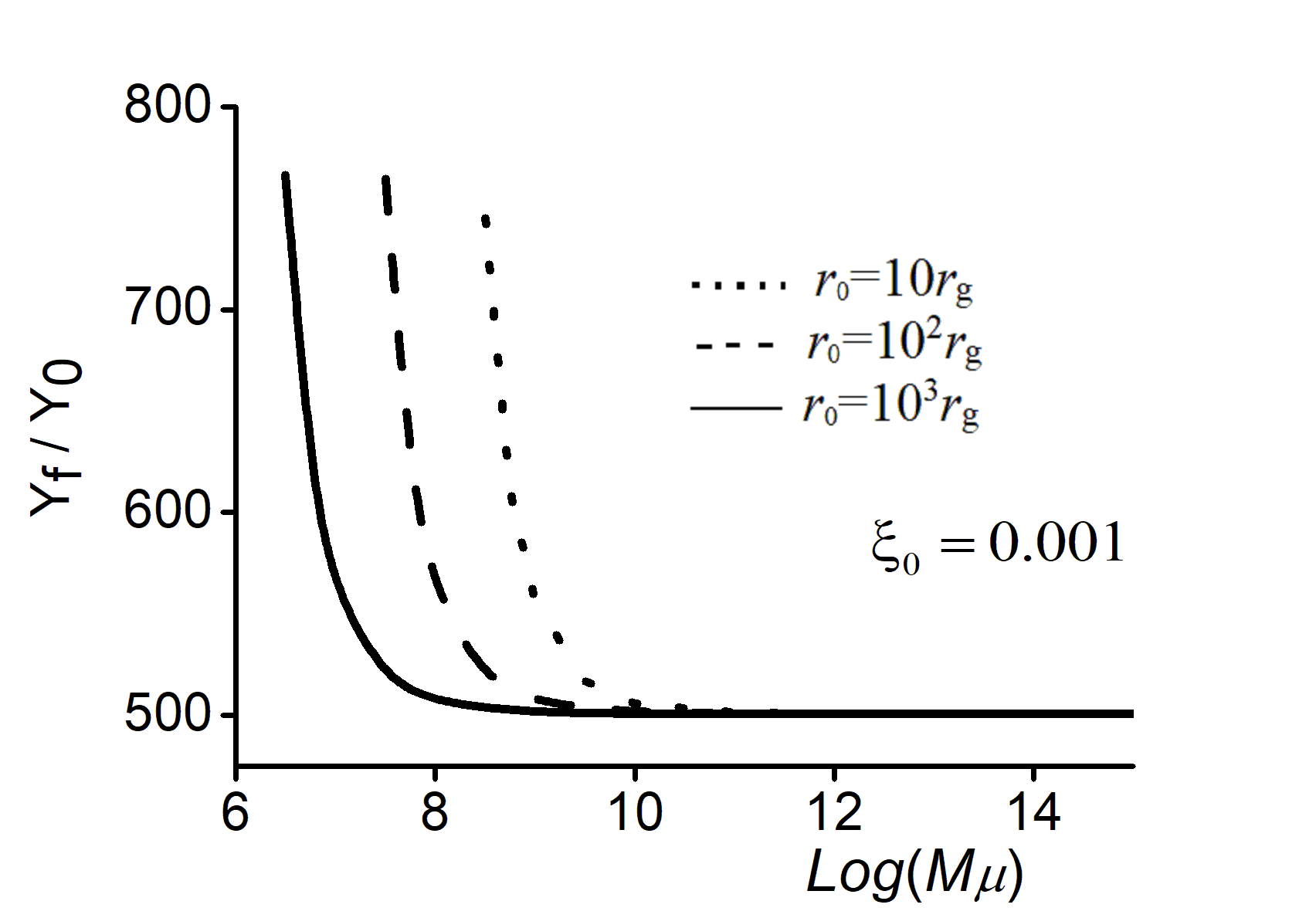
Figure 1: The case of potential (43): dependence of limiting value $Y_{f}/Y_{0}$ upon $M\mu$ for three sizes $r_{0}$ of the scalarization region determined by condition $\xi(r_{0})=0.001$. Dotted line ($r_{0}=10r_{g}$) corresponds to $\log(Q)\approx 4.8\mu r_{g}$; dashed ($r_{0}=10^{2}r_{g}$) – to $\log(Q)\approx 44.4\mu r_{g}$; solid ($r_{0}=10^{3}r_{g}$) – to $\log(Q)\approx 435.8\mu r_{g}$.

VII Discussion

We studied asymptotically flat SSS configurations in the Einstein frame of the $f(R)$ gravity with potentials satisfying conditions (6),(7),(8) that are typical for a number of known $f(R)$ gravity models. We found a representation of the equations that describe the SSS configuration that allowed us to derive approximate solutions and to perform numerical calculations for rather high values of $M\mu=10^{6}\div 10^{50}$.

For large enough $M\mu$, the SSS solutions exhibit remarkably similar behavior for $f(R)$ models satisfying (6),(7),(8). There are three main regions of the radial variable with different types of behavior of every SSS solution.

Region A. Here we have small scalaron field that decays exponentially according to (12) as $r$ grows. The metric and, accordingly, the distribution of circular orbits are practically the same as in the case of the Schwarzschild metric. We typically considered this region according to $r>r_{0}$ with $r_{0}=(10\div 1000)r_{g}$; although this does not seem to limit our qualitative findings. However, if such $f(R)$ structures really exist, then the value of $r_{0}$ is unlikely to be very large, since objects with a large scalarization region could somehow manifest themselves in observations.

Region B. This is a small ($\Delta r\sim l_{\mu}$) transition region from A to C with a strong jump-like variation of essential parameters.

Region C. This is a region of strong scalaron field ($r\lesssim r_{0}$); here the qualitative behavior of the solution is significantly different from the Schwarzschild case. For large $M\mu$ we have practically constant values of $rd\xi/dr$ and $r\exp((\alpha-\beta)/2)$ right up to the naked singularity at the origin. This enables us to write explicit approximate expressions for the scalaron field and for the metric coefficients in the Einstein and Jordan frames (40), (41),(42). One can easily deduce from (41),(42) that there are no circular orbits in region C, and no evidence of an accretion disk should be expected.

Thus we have an approximate solution, which satisfactory describes static spherically symmetric configuration of the $f(R)$ gravity for sufficiently large $M\mu$; the larger $M\mu$, the better is the accuracy of the approximation.

Our findings relate to vacuum solutions of the $f(R)$ gravity. However, our results can be applied to the case where a non-zero spherically symmetric continuous distribution of mass-energy is present in the central region. In this case, the gravitational field in the interior region is determined by the energy-momentum tensor inside the body. Outside this body, the field is completely determined by total configuration mass $M$ and the “scalar charge” $Q$ after appropriate matching with the internal region.

Acknowledgements. I am grateful to Yu. Shtanov and O. Stashko for useful discussions. This work was supported by the National Research Foundation of Ukraine under project No. 2023.03/0149.

References

- Sotiriou and Faraoni [2010] T. P. Sotiriou and V. Faraoni, theories of gravity, Reviews of Modern Physics 82, 451 (2010), arXiv:0805.1726 [gr-qc] .
- De Felice and Tsujikawa [2010] A. De Felice and S. Tsujikawa, theories, Living Reviews in Relativity 13, 3 (2010), arXiv:1002.4928 [gr-qc] .
- Nojiri et al. [2017] S. Nojiri, S. D. Odintsov, and V. K. Oikonomou, Modified gravity theories on a nutshell: Inflation, bounce and late-time evolution, Phys. Rept. 692, 1 (2017), arXiv:1705.11098 [gr-qc] .
- Starobinsky [1980] A. A. Starobinsky, A new type of isotropic cosmological models without singularity, Phys. Lett. B 91, 99 (1980).
- Vilenkin [1985] A. Vilenkin, Classical and quantum cosmology of the Starobinsky inflationary model, Phys. Rev. D 32, 2511 (1985).
- Starobinsky [2007] A. A. Starobinsky, Disappearing cosmological constant in f(R) gravity, Soviet Journal of Experimental and Theoretical Physics Letters 86, 157 (2007), arXiv:0706.2041 [astro-ph] .
- Shtanov et al. [2023] Y. Shtanov, V. Sahni, and S. S. Mishra, Tabletop potentials for inflation from gravity, J. Cosmol. Astroparticle Phys. 03, 023 (2023), arXiv:2210.01828 [gr-qc] .
- Nojiri and Odintsov [2003] S. Nojiri and S. D. Odintsov, Modified gravity with negative and positive powers of curvature: Unification of inflation and cosmic acceleration, Phys. Rev. D 68, 123512 (2003).
- Appleby and Battye [2008] S. A. Appleby and R. A. Battye, Aspects of cosmological expansion in F(R) gravity models, JCAP 2008 (5), 019, arXiv:0803.1081 [astro-ph] .
- Oikonomou and Giannakoudi [2022] V. K. Oikonomou and I. Giannakoudi, A panorama of viable f(r) gravity dark energy models, International Journal of Modern Physics D 31, 2250075 (2022), https://doi.org/10.1142/S0218271822500754 .
- Amendola and Tsujikawa [2015] L. Amendola and S. Tsujikawa, Dark Energy (2015).
- Capozziello et al. [2006] S. Capozziello, V. F. Cardone, and A. Troisi, Dark energy and dark matter as curvature effects, J. Cosmol. Astroparticle Phys. 08, 001 (2006), arXiv:astro-ph/0602349 .
- Cembranos [2009] J. A. R. Cembranos, Dark matter from gravity, Phys. Rev. Lett. 102, 141301 (2009), arXiv:0809.1653 [hep-ph] .
- Cembranos [2016] J. A. R. Cembranos, Modified gravity and dark matter, J. Phys. Conf. Ser. 718, 032004 (2016), arXiv:1512.08752 [hep-ph] .
- Corda et al. [2012] C. Corda, H. J. Mosquera Cuesta, and R. Lorduy Gomez, High-energy scalarons in gravity as a model for Dark Matter in galaxies, Astropart. Phys. 35, 362 (2012), arXiv:1105.0147 [gr-qc] .
- Katsuragawa and Matsuzaki [2017] T. Katsuragawa and S. Matsuzaki, Dark matter in modified gravity?, Phys. Rev. D 95, 044040 (2017), arXiv:1610.01016 [gr-qc] .
- Katsuragawa and Matsuzaki [2018] T. Katsuragawa and S. Matsuzaki, Cosmic history of chameleonic dark matter in gravity, Phys. Rev. D 97, 064037 (2018), [Erratum: Phys. Rev. D 97, 129902 (2018)], arXiv:1708.08702 [gr-qc] .
- Yadav and Verma [2019] B. K. Yadav and M. M. Verma, Dark matter as scalaron in gravity models, J. Cosmol. Astroparticle Phys. 10, 052 (2019), arXiv:1811.03964 [gr-qc] .
- Parbin and Goswami [2021] N. Parbin and U. D. Goswami, Scalarons mimicking dark matter in the Hu–Sawicki model of gravity, Mod. Phys. Lett. A 36, 2150265 (2021), arXiv:2007.07480 [gr-qc] .
- Shtanov [2021] Y. Shtanov, Light scalaron as dark matter, Physics Letters B 820, 136469 (2021), arXiv:2105.02662 [hep-ph] .
- Kapner et al. [2007] D. J. Kapner, T. S. Cook, E. G. Adelberger, J. H. Gundlach, B. R. Heckel, C. D. Hoyle, and H. E. Swanson, Tests of the gravitational inverse-square law below the dark-energy length scale, Phys. Rev. Lett. 98, 021101 (2007), arXiv:hep-ph/0611184 .
- Adelberger et al. [2007] E. G. Adelberger, B. R. Heckel, S. A. Hoedl, C. D. Hoyle, D. J. Kapner, and A. Upadhye, Particle-physics implications of a recent test of the gravitational inverse-square law, Phys. Rev. Lett. 98, 131104 (2007), arXiv:hep-ph/0611223 .
- Hernandéz-Lorenzo and Steinwachs [2020] E. Hernandéz-Lorenzo and C. F. Steinwachs, Naked singularities in quadratic gravity, Phys. Rev. D 101, 124046 (2020), arXiv:2003.12109 [gr-qc] .
- Zhdanov et al. [2024] V. I. Zhdanov, O. S. Stashko, and Y. V. Shtanov, Spherically symmetric configurations in the quadratic f (R ) gravity, Phys. Rev. D 110, 024056 (2024), arXiv:2403.16741 [gr-qc] .
- Asanov [1968] R. A. Asanov, Static scalar and electric fields in Einstein’s theory of relativity, Soviet Journal of Experimental and Theoretical Physics 26, 424 (1968).
- Asanov [1974] R. A. Asanov, Point source of massive scalar field in gravitational theory, Theoretical and Mathematical Physics 20, 667 (1974).
- Rowan and Stephenson [1976] D. J. Rowan and G. Stephenson, The massive scalar meson field in a Schwarzschild background space, Journal of Physics A Mathematical General 9, 1261 (1976).
- Zhdanov and Stashko [2020] V. I. Zhdanov and O. S. Stashko, Static spherically symmetric configurations with nonlinear scalar fields: Global and asymptotic properties, Phys. Rev. D 101, 064064 (2020), arXiv:1912.00470 [gr-qc] .
- Akrami et al. [2020] Y. Akrami et al. (Planck Collaboration), Planck 2018 results. X. Constraints on inflation, Astron. Astrophys. 641, A10 (2020), arXiv:1807.06211 [astro-ph.CO] .