Economic Geography and Structural Change

Abstract

As countries develop, the relative importance of agriculture declines and economic activity becomes spatially concentrated. We develop a model integrating structural change and regional disparities to jointly capture these phenomena. A key modeling innovation ensuring analytical tractability is the introduction of non-homothetic Cobb-Douglas preferences, which are characterized by constant unitary elasticity of substitution and non-constant income elasticity. As labor productivity increases over time, economic well-being rises, leading to a declining expenditure share on agricultural goods. Labor reallocates away from agriculture, and industry concentrates spatially, further increasing aggregate productivity: structural change and regional disparities are two mutually reinforcing outcomes and propagators of the growth process.

Keywords: New Economic Geography, Structural Change, Non-Homothetic Preferences.

JEL Codes: D11, F11, O40, R10.

1 Introduction

The geographic and sectoral distributions of economic activity jointly evolve along the development path. Figure 1 shows how, as income per capita grows, the share of value added in agriculture declines (Figure 1a) and the share of population in urban areas increases (Figure 1b) for a panel of 38 countries spanning very different income levels. Combining these two patterns, Figure 1c shows a strong, negative correlation between agricultural value added shares and spatial concentration of economic activity as proxied by urbanization rates. What is the relationship between structural change and spatial concentration? Does one drive the other or are they jointly determined? Are there any feedback effects between them?

The purpose of this paper is to provide a parsimonious framework to analyze these questions, bringing together elements of economic geography and structural change. In particular, we combine an economic geography framework with a demand-driven theory of structural change in which we introduce a novel non-homothetic demand system – “Heterothetic Cobb-Douglas” (henceforth hcd). These preferences feature a variable income elasticity of demand while maintaining a constant, unitary elasticity of substitution. This combination of elements (particularly, the unitary elasticity of substitution) results in a tractable unified framework that enables us to study a rich set of two-way interactions between structural change and the evolution of regional disparities. Our central result is to show how rising incomes yield spatial concentration through structural change, and how rising spatial concentration increases incomes, fueling structural change. Importantly, our framework allows us to show how both structural change and spatial concentration arise as an outcome of economic growth, without needing a fall in transportation and trade costs. The theory can also shed light on the evolution of earnings inequality.

Figure 1: The Joint Evolution of Agricultural and Urban Economic Activity

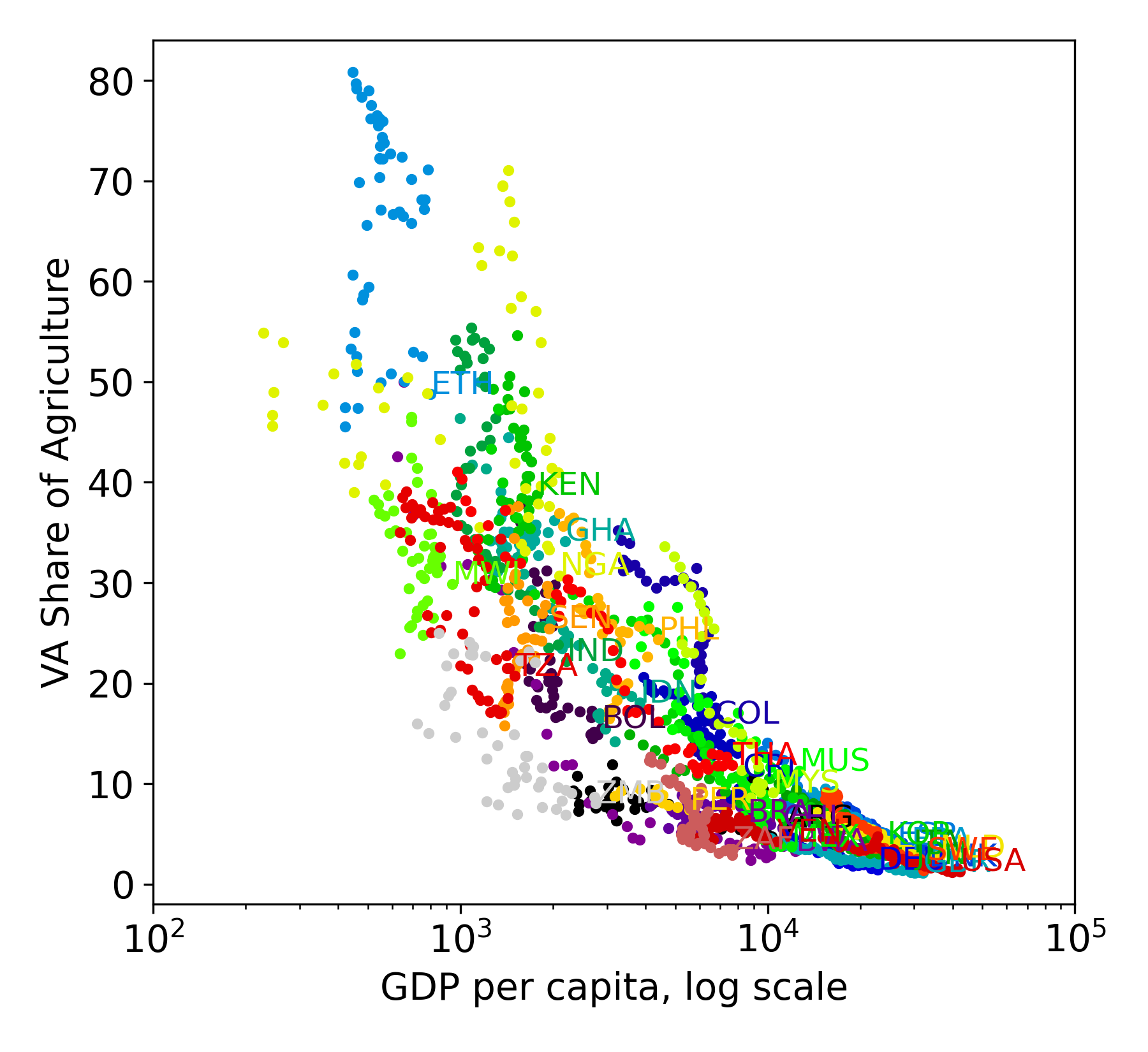
(a) Agricultural Shares and Income pc

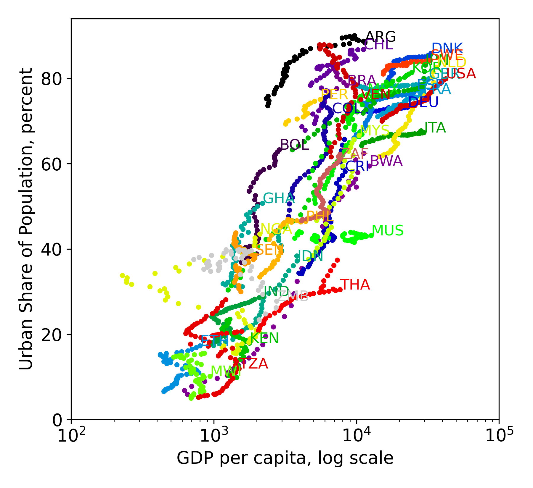
(b) Urbanization and Income pc

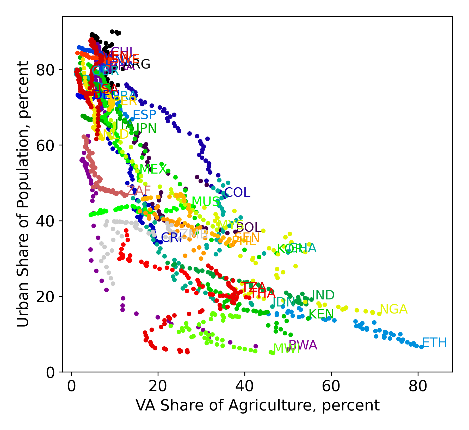
(c) Agri. Shares and Urbanization

Notes: Data for agricultural value-added shares comes from the Groningen 10-sector database as computed in Comin, Lashkari, and Mestieri (2021). Urbanization rates comes from the United Nations Urban Indicators Database. Income per capita corresponds to 2017 US dollars (PPP-adjusted) from the PWT. See Appendix E for more details.

For simplicity, we consider only two factors of production, two sectors, and two regions endowed with identical fundamentals, as in the seminal “new” economic geography (henceforth neg) paper by Krugman (1991). The factors are labor (owned by “workers”) and human capital (owned by “entrepreneurs”). We label the sectors agriculture and manufacturing, where manufacturing lumps together the manufacturing and service industries. In line with empirical evidence, the income elasticity of demand for this composite good is larger than one, hence its share in national income increases as real income per capita grows over time. Conversely, agriculture is a necessity, and its share in employment and in national income falls over time: the economy undergoes a structural transformation (see, e.g., Caselli and Coleman II, 2001, and Kongsamut, Rebelo, and Xie, 2001).

In our model, agriculture is tied to the land, and the workers it employs are a source of geographically immobile demand for the composite good; this so-called dispersion force tends to disperse economic activity across space. Conversely, entrepreneurs are mobile and the manufacturing firms they manage tend to move to the region with the larger demand to save on trade and transportation costs; in turn, the region with the larger demand tends to be the one hosting the most entrepreneurs since they also consume manufacturing goods. Thus, the larger their expenditure share on manufacturing, the stronger this positive feedback loop, and the more likely these self-enforcing agglomeration economies dominate dispersion forces leading to the spatial concentration of manufacturing in equilibrium. This expenditure share in manufacturing is a key parameter in Krugman’s core-periphery model. In our model, by contrast, it is an endogenous outcome that depends on the income level of the economy. As we explain below, unlike the fall of transportation costs, whose impact on regional disparities depends on subtle modeling assumptions, the rise of labor productivity and of the equilibrium expenditure share on manufacturing has an unambiguous impact on the emergence of regional disparities. In particular, regional disparities are an equilibrium outcome regardless of the level of transportation costs if labor productivity and the equilibrium expenditure share on manufacturing are high enough. The endogenous emergence of such a “black hole” cannot arise in original neg models featuring homothetic preferences and constant expenditure shares.

Our framework highlights the two-way relationship between regional disparities and structural change: growth-led structural change generates regional disparities, and the emergence of regional disparities induces further structural change. Consider the following thought experiment. Assume that labor productivity is initially low: the economy is predominantly agricultural and manufacturing firms are evenly dispersed across regions at the unique stable equilibrium. As labor productivity monotonically increases over time, per capita incomes and economic well-being rises. In turn, due to the non-homothetic demand system, the share of spending on manufactures increases and that on agriculture falls. The first implication of this process is that labor reallocates from agriculture to manufacturing: structural change unfolds.

As the share of spending on manufactures increases, a second implication is that agglomeration forces strengthen and dispersion forces weaken since entrepreneurs benefit from locating in the same region. Eventually, the spatial concentration of manufacturing becomes the only stable equilibrium outcome: regional disparities emerge. This result illustrates how structural change fuels regional disparities, and it is thus unlikely to happen uniformly across space. Industrialization may only take place in a few “cores” (Puga and Venables, 1996). Furthermore, the spatial concentration of manufacturing exerts a positive feedback effect on income growth and structural change. As industry concentrates geographically, the price of the consumption basket of manufacturing falls for the entrepreneurs – since by consuming in the same location of production, they minimize the trade and transportation costs. As a result, the utility levels of entrepreneurs increase and, since manufacturing is a luxury, their expenditure share on manufacturing increases. This mechanism illustrates how spatial concentration of manufacturing fuels income growth and structural change.

Finally, structural change brought about by the combination of steady growth of labor productivity and of manufacturing being a luxury good also has an effect on income inequality. Though economic growth benefits both types of factor owners, productivity growth disproportionately benefits the owners of the factor used intensively in the sector growing the most – entrepreneurs. This logic is well-known since at least Jones (1965), and here it extends to the case of a factor-specific model featuring monopolistic competition.

2 Relation to the Literature

Our paper combines elements from the fields of economic geography and from structural change.

The first major ingredient of our model borrows from the arguably no-longer aptly named “new” economic geography. It features two regions with identical fundamentals, some geographically mobile factors, monopolistic competition, scale economies, and trade and transportation costs, as in Krugman (1991) and in the vast literature that followed (Baldwin, Forslid, Martin, Ottaviano, and Robert-Nicoud, 2003; Fujita, Krugman, and Venables, 1999). Under some conditions, the combination of these ingredients gives rise to self-enforcing agglomeration economies and to the emergence of regional disparities. The basic structure of Krugman’s model is simple but its analysis is complex, and it took fifteen years and combined efforts of several authors to complete a comprehensive analysis of standard neg models. Even though we add one source of complexity to this framework – non-homothetic preferences – our model does so in a relatively parsimonious way. It encompasses the variant of Krugman’s model introduced by Forslid and Ottaviano (2003) as a special case (when preferences are homothetic Cobb-Douglas). Our paper also complements the works of Baldwin, Martin, and Ottaviano (2001), who study how innovation and growth interact in an neg framework, and of Ottaviano, Tabuchi, and Thisse (2002) and Pfluger (2004), who introduce neg models with quasi-linear (and hence non-homothetic) preferences. Both models are analytically more amenable than Krugman’s original. However, manufacturing is a necessity and agricultural goods are a luxury in these models, which is counterfactual.

Krugman’s original focus, as well as that of much of the neg literature’s, was on the role of trade and transportation costs in fostering regional disparities. This focus resonated to Europeans in particular, as it shed light on the European Single Market Program from an original angle at the time. The economic mechanisms unveiled by the neg suggest that globalization and European economic integration may contribute to deepening of regional disparities rather than fostering spatial convergence (Puga, 2002). In this paper, we shift the narrative by demonstrating that falling transportation costs are neither necessary nor even likely to be the main driver of regional disparities. Rather, our analysis emphasizes that structural change associated with economic growth induces regional disparities on its own.

This approach addresses two critiques of Krugman’s original model. First, Helpman (1998) includes consumption of housing (a non-traded service) instead of agriculture (a freely traded good in Krugman’s model) in his alternative neg model. Helpman shows that competition among mobile workers for this non-tradable service contributes to regional convergence, and that falling transportation costs actually amplify this dispersion force: trade integration does not cause regional disparities; quite the opposite, it contributes to regional convergence. Our theory is robust to Helpman’s critique, as increasing agglomeration forces are driven by a rising expenditure share in the good that exhibits increasing returns to scale – manufacturing – and this force persists even when land is included, as long as housing is a necessity (which is empirically the case).

Second, Krugman himself nuanced the findings of his paper, by emphasizing that his model features a region of the parameter space (when the expenditure share on the sector featuring economies of scale is sufficiently large) that implies the emergence of regional disparities in equilibrium regardless of the level of transportation costs. He addressed this caveat by introducing the “No Black-Hole Condition” ruling out this outcome by assumption. From the perspective of our paper with endogenous expenditure shares, the black hole becomes an equilibrium outcome, and therefore a feature of the model rather than a bug. As labor productivity rises and the expenditure share on manufacturing consequently increases, the economy transitions from having no regional disparities, to having the potential of regional disparities, to inevitably featuring regional disparities in equilibrium, i.e. the black hole. An important implication of this results is that prohibitive transportation costs in a sector are not inconsistent with its spatial clustering. Our model can thus accommodate the agglomeration of non-traded services as an equilibrium outcome.

The second major ingredient of our model is demand-driven structural change: expenditure and resources reallocate away from agriculture as economic well-being rises. Dennis and Iscan (2009) document a preponderant role of income effects in the United States’ structural change out of agriculture from 1800 to 1950. We deliberately switch-off the relative price-effect channel by setting the elasticity of substitution between manufacturing and agriculture to one. Thus, for any given fixed level of utility, any form of technical progress on the supply side leaves expenditure shares and employment shares unchanged. It would be conceptually straightforward to extend the analysis of our paper to allow this channel to operate by using the non-homothetic constant elasticity of substitution (nh-ces) to model structural change (Comin, Lashkari, and Mestieri, 2021) in a spatial context as in Finlay and Williams (2022) and Takeda (2022). Such an extension is ancillary to the main point we make here: economic growth is a source of both structural change and regional disparities when preferences are non-homothetic.

Our paper contributes to the growing literature that studies structural change and economic geography jointly. A few of these papers also use non-homothetic preferences. The closest paper to ours is Murata (2008), who uses Stone-Geary preferences (Geary, 1950; Stone, 1954) in an otherwise standard two-region neg model. His analysis focuses on the role of trade and transportation costs, as do most neg contributors. Caselli and Coleman II (2001) show that structural transformation is a source of regional income convergence in neoclassical models in the presence of decreasing marginal returns of mobile factors of production and in the absence of trade costs among regions. They also use Stone-Geary preferences, which feature non-unitary income and price elasticities of demand. By contrast, Chatterjee, Giannone, Kleineberg, and Kuno (2024) document that regional convergence has stalled since the 1980s for a panel of 34 countries and relate it to the rise of the service sector. Eckert and Peters (2022) and Budi-Ors and Pijoan-Mas (2022) build quantitative spatial general equilibrium models to study the spatial dimension of structural change in the United States at the turn of the twentieth century (Eckert and Peters, 2022) and in Spain from 1940 to 2000 (Budi-Ors and Pijoan-Mas, 2022). Caselli and Coleman II (2001), Budi-Ors and Pijoan-Mas (2022) and Chatterjee, Giannone, Kleineberg, and Kuno (2024) use Stone-Geary preferences, which, like all explicitly additively separable preferences, display fundamental flaws (Matsuyama, 2016). The hcd preferences we use to model structural change do not suffer from these flaws. Eckert and Peters (2022) follow Boppart (2014) in using price-independent generalized linear (pigl) preferences. These preferences have more desirable properties than Stone-Geary preferences while maintaining aggregation, but they only accommodate two sectors. By contrast, our hcd preferences are a limiting case of nh-ces preferences; they accommodate an arbitrary number of goods and sectors and have a constant unitary price elasticity. They also yield a “generalized separable” demand system (Fally, 2022; Gorman, 1995; Pollak, 1972). We anticipate that hcd preferences will be of independent interest and applied to a wide range of contexts.

3 Heterothetic Cobb-Douglas Preferences

We begin by characterizing hcd preferences in their general form after which we introduce them to the NEG model of spatial and structural change. All proofs are contained in the appendix.

Consider the utility function $U:\times_{i\in I}\left[\gamma_{i},\infty\right)\mapsto\left(1,\infty\right)$ that maps the consumption vector $\left\{C_{i}\right\}_{i\in I}$ into a level of utility $u$, where $u$ is implicitly defined by:

$$\ln u=\sum_{i}\omega_{i}\left(u\right)\ln\left(\frac{C_{i}}{\gamma_{i}}\right)-\sum_{i}\omega_{i}\left(u\right)\ln\left(\frac{\omega_{i}\left(u\right)}{\omega(u)}\right),$$ (1)

and where $\omega(u)\equiv\sum_{i}\omega_{i}(u)$. The parameter $\gamma_{i}$ defines some minimal amount of good $i$ over which $U$ is defined. The distinction from homothetic Cobb-Douglas is that the weights $\omega_{i}$ are a no longer a parameter, but a function of the utility level $u$. We impose the following regularity conditions on these weight functions, which ensure interior solutions for the utility maximization program, and in turn that the expenditure and indirect utility functions are well-behaved:

Assumption 1.

Self-Consistency. There exist real numbers $\{\text{\text@underline{s}}_{i}\}\in(0,1)$, such that $\forall i\in I,\forall u\geq 1$: (i) $\text{\text@underline{s}}_{i}\leq\frac{\omega_{i}(u)}{\omega(u)}$, (ii) $\partial\omega_{i}/\partial u\leq 0$ (with strict inequality for at least one good), and (iii) the vector of prices and income $\left(\left\{P_{i}\right\},y\right)$ obeys

$$P_{i}\gamma_{i}<\uline{s}_{i}y.$$ (2)

Parts (i) and (iii) of this assumption together ensure that the share of income that the preferences imply should be allocated to any given good exceeds the minimum required level of expenditures for that good $P_{i}\gamma_{i}$. Without the assumption, the preferences may be internally inconsistent, requiring a level of consumption on a good that is higher than the expenditure share the preferences imply should be allocated toward it. The assumption also implies a limit on the realized variance of prices, which are an endogenous outcome. Generally, one would have to make assumptions on fundamentals that ensure that this inequality is verified in equilibrium, and we will highlight the needed parameter restrictions below (see Lemma 7). In the limiting case of $\gamma_{i}\rightarrow 0$, however, this inequality is verified as long as prices remain finite. This case imposes the most minimalist residual restrictions, and we therefore make the following assumption:

Assumption 2.

Regularity conditions. $\forall i\in I:\gamma_{i}\in\mathbb{R}_{++}$. We choose units of measurement for these goods so that $\gamma_{i}=\gamma$ for all $i\in I$, and let $\gamma\rightarrow 0$, in which case $U$ is defined almost everywhere. For simplicity, we will also assume that $\uline{s}_{i}=\uline{s}$ for all $i\in I$.

Existence and global convexity of the function $U$.

Note that the requirement $C_{i}\geq\gamma$ and assumptions 1 and 2 together imply that $\ln\left(\frac{\omega C_{i}}{\omega_{i}\gamma}\right)>0$ holds for any good $i$, and that the right-hand side of equation (1) is decreasing in $u$. We obtain the following result.

Lemma 3.

Regularity conditions. Assume preferences obey equation (9), and assumptions 1 and 2 hold; then in equilibrium (i) $C_{i}>\gamma$ and (ii) $\nicefrac{{\partial u}}{{\partial C_{i}}}>0$ for all $i\in I$.

Indirect utility and expenditure functions.

The indirect utility function $V:\times_{i}\left(0,\infty\right)\mapsto\left(1,\infty\right)$, maps the vector of prices and income $\left(\left\{P_{i}\right\},y\right)$ into a level of utility. Under assumptions 1 and 2, which we maintain throughout the paper as they ensure an interior solution, the optimal consumption allocations under hcd preferences imply relative expenditure shares that are proportional to the the relative preference weights, as is the case under homothetic Cobb-Douglas. We can therefore define and write expenditure shares as

$$m_{i}\left(u\right)\equiv\frac{P_{i}C_{i}}{y}=\frac{\omega_{i}\left(u\right)}{\omega\left(u\right)}.$$ (3)

To obtain the indirect utility function, plug $C_{i}=\frac{\omega_{i}y}{\omega P_{i}}$ and $v=u$ into (1) to get:

$$\ln v=\sum_{i}\omega_{i}\left(v\right)\ln\left(\frac{y}{\gamma P_{i}}\right).$$ (4)

The derivative of the left hand side in the expression above with respect to $v$ is positive by inspection, while the derivative of its right-hand side is negative by assumptions 1 and 2. It then follows from $\omega_{i}>0$ that $v$ is increasing in $y$ and decreasing in $P_{i}$. We can then establish the following results:

Lemma 4.

Indirect utility function. Assume assumptions 1 and 2 hold. Then the indirect utility $V\left(\{P_{i}\},y\right)$ associated with the preferences in equation (1) can be written implicitly as the fixed point for $v$ of expression (4). This fixed point exists and is unique. Furthermore, $V$ is increasing in $y$, decreasing in $P_{i}$, and homogeneous of degree zero in its arguments. Hence $V$ is a proper indirect utility function.

Lemma 5.

Expenditure function. Assume assumptions 1 and 2 hold. Then the expenditure function $E\left(u,\{P_{i}\}\right)$ associated with the preferences in equation (1) can be written as:

$$\ln E\left(u,\{P_{i}\}\right) =\ln\Omega\left(u\right)+\sum_{i}m_{i}\left(u\right)\ln\left(P_{i}\right),$$ (5)

where

$$\ln\Omega\left(u\right)\equiv\ln\gamma+\frac{\ln u}{\omega\left(u\right)}.$$ (6)

The function $E$ is increasing in its arguments and it is homogeneous of degree one in prices. Hence $E$ is a proper expenditure function.

Equating expenditure with nominal income $y$, it follows from equation (5) that we can naturally interpret $\Omega$ as the real income: $\Omega=y/\mathbb{P}$, where $\ln\mathbb{P}\equiv\sum_{i}m_{i}\left(u\right)\ln\left(P_{i}\right)$ is a (utility-dependent) price index. Notably, this price index is computable with readily observable data: expenditure shares and prices. It follows from $u>1$ and $\omega^{\prime}<0$ that $\Omega$ is monotonically increasing in $u$. Since utility is an ordinal concept, we can interchangeably use $u$ or $\Omega$ as our metric for utility. We will make use of this property in section 5 below.

4 A Two-Region Model of Spatial and Structural Change

After having introduced hcd preferences, we now present our application to a model of spatial and structural changes. Our full model is a succession of static equilibriums in which growth is driven by exogenous increases in labor productivity. We begin by presenting the static equilibrium in this section and next. To maximize analytical tractability, the static model follows the structure of Forslid and Ottaviano (2003), a more analytically tractable variant of Krugman’s seminal 1991 paper, as closely as possible.

Model Overview

The economy consists of two regions, $r,s\in\left\{1,2\right\}$, and two sectors, agriculture and manufacturing $i\in\{A,M\}$. Agricultural production is a constant returns to scale sector that is tied to the land. It produces a homogeneous good competitively and its output is traded at no cost between the two regions. Manufacturing consists of differentiated goods produced under increasing returns that are internal to each firm. Each firm produces a different variety. Market conduct is monopolistically competitive as in Dixit and Stiglitz (1977). Manufacturing firms may locate in either region, and their output is traded at a cost, which takes the standard iceberg form, as in Samuelson (1954). There are two factors of production, labor (workers), and human capital (entrepreneurs). Workers are geographically immobile but they may work in either sector, as in Forslid and Ottaviano (2003). We normalize the mass of workers to one, so there is a mass of $\frac{1}{2}$ workers in each region. We denote their wage by $w^{r}$. Entrepreneurs manage manufacturing firms and may move across regions in search of the highest real returns. We also normalize the mass of entrepreneurs to one, and denote by $\lambda^{r}$ the share of entrepreneurs who live and produce in region $r$ and denote their nominal earnings by $\pi^{r}$. Finally, we denote the prices of the agriculture good and of the composite manufacturing good by $P_{A}$ and $P_{M}$, respectively.

4.1 Production and Trade Technologies

Agricultural Technology.

The production technology for agriculture is linear in labor $A^{r}=\alpha L_{A}^{r},$ where $A^{r}$ and $L_{A}^{r}$ denote output and labor input in region $r$, and $\alpha>1$ is the marginal product of labor in agriculture.

Manufacturing Technology.

Each manufacturing firm produces a differentiated variety and is run by a single manager. Labor is the sole variable input. Let $\mu>0$ denote the marginal product of labor in manufacturing and $\pi^{r}$ the nominal earnings of the entrepreneur running the firm. The cost function of an arbitrary manufacturing firm established in region $r$ and producing $x$ units of output is

$$c^{r}\left(x\right)=\pi^{r}+\frac{w^{r}}{\mu}x.$$ (7)

Trade Technology.

Agricultural output is freely traded and is produced in both regions. By contrast, trade in manufactures is costly. Firms may ship their output at no cost within their own region, but need to ship $\tau>1$ units of output for one unit to arrive in the other region (the rest melts in transit). We henceforth refer to $\tau$ as “trade costs” for short, which encapsulates any physical or legal cost borne from conducting inter-regional trade.

4.2 Endowments and Preferences

Workers.

Each worker is endowed with one unit of labor that is inelastically supplied. Workers consume manufacturing goods only. The utility they derive from consuming manufacturing varieties is a constant-elasticity-of-substitution (CES) aggregate $C_{M}$,

$$C_{M}=\left[\int_{0}^{N}\left(c\left(n\right)\right)^{\frac{\sigma-1}{\sigma}}dn\right]^{\frac{\sigma}{\sigma-1}},$$ (8)

where $\sigma>1$ is the elasticity of substitution, and $N$ is the endogenous mass of active firms, which is pinned down in equilibrium.

Entrepreneurs.

Entrepreneurs are endowed with one unit of human capital, which they use to run firms. Entrepreneurs hold two-tiered preferences. The upper tier is defined over the agricultural and composite manufacturing good, and the lower tier is defined over manufacturing varieties with the same ces aggregator $C_{M}$ in equation (8) as for workers. For the upper tier, entrepreneurs have hcd preferences over agriculture and manufacturing as laid out in the previous section. The utility function $U:\times_{i\in\left\{A,M\right\}}\left[\gamma,\infty\right)\mapsto\left(1,\infty\right)$ maps the consumption vector $\left\{C_{A},C_{M}\right\}$ into a level of utility $u$ implicitly defined by

$$\ln u=\omega_{A}\left(u\right)\ln\left(\frac{C_{A}}{\gamma}\right)+\omega_{M}\left(u\right)\ln\left(\frac{C_{M}}{\gamma}\right)-\sum_{i\in A,M}\omega_{i}(u)\ln\left(\frac{\omega_{i}(u)}{\omega(u)}\right).$$ (9)

As discussed in Section 3, the associated expenditure function is

$$\ln E\left(P_{A},P_{M},u\right) =\ln(\Omega\left(u\right))+m\left(u\right)\ln\left(P_{M}\right)+(1-m(u))\ln(P_{A}).$$ (10)

In order to have the manufacturing composite good be a luxury and the agricultural good be a necessity, we impose the additional assumption:

Assumption 6.

Manufacturing is a luxury. $\frac{\omega_{M}}{\omega_{A}}$ is increasing everywhere in $u$.

It follows from assumptions 1(i) and 6 that the expenditure share on manufactures belongs to the interior of the unit interval and is increasing in $u$:

$$\forall u\in\left(1,\infty\right):\qquad 0<m\left(u\right)<1,\quad 0<m^{\prime}\left(u\right).$$ (11)

4.3 Markets and Equilibrium conditional on Location Choices

Agriculture.

The market for the agricultural good is competitive. Hence, in any equilibrium the law of one price holds. The agricultural good is then a natural choice for numeraire, and we set $P_{A}=1$. Marginal cost pricing and the absence of trade and transportation costs together imply that

$$w^{r}=\alpha.$$ (12)

Henceforth, we refer to parameter $\alpha$ as “labor productivity.” An increase in $\alpha$ rises labor productivity in the agricultural sector and, ultimately, the equilibrium wage for labor in the economy. Labor productivity will be a central parameter of interest in the analysis of spatial structural change.

Manufacturing.

Manufacturing operates under monopolistic competition. Markets are segmented and firms set prices in both regions $r\in\left\{1,2\right\}$ independently. Since all firms are managed by exactly one manager, all managers are fully employed in equilibrium, hence $N=1$. The combination of ces preferences among manufactures on the demand side and monopolistic competition with segmented markets on the supply side gives rise to the equilibrium f.o.b. prices $p^{r}=\frac{\sigma}{\left(\sigma-1\right)\mu}w^{r}$. Without loss of generality, we set $\mu=\frac{\alpha\sigma}{\sigma-1}$ so that the equilibrium f.o.b. price is equal to

$$p^{r}=1,\qquad\forall r\in\left\{1,2\right\}.$$ (13)

Due to trade costs, the location and pricing decisions of firms affect the price index for the composite manufacturing good, $P_{M}^{r}$. Workers and atomistic entrepreneurs take as given the location of firms as characterized by the density of entrepreneurs in each region $\left\{\lambda^{r},1-\lambda^{r}\right\}$. This results in a region-specific manufacturing price-index, $P_{M}^{r}$, which is a generalized weighted average of consumer prices:

$$\left(P_{M}^{r}\right)^{1-\sigma}=\lambda^{r}+\left(1-\lambda^{r}\right)\tau^{1-\sigma},$$ (14)

where we use the normalization that there is no trade costs for shipments to the own region.

Individual consumer prices are equal to producer prices for the domestically produced varieties and to $\tau$ times the producer price for varieties that are imported from region $r\neq s$.

Equilibrium Earnings, Sales, and Expenditures.

Let $R^{r}\equiv p^{r}x$ and $\Pi^{r}\equiv R^{r}-c^{r}$ respectively denote revenue and profits of a representative firm in region $r$ producing output $x$. Using $\mu=\frac{\alpha\sigma}{\sigma-1}$, as well as equations (7) and (13), we obtain $\Pi^{r}=-\pi^{r}+\frac{R^{r}}{\sigma}$. By free entry, firm owners compete for entrepreneurs until profits are exhausted ($\Pi^{r}=0$), so that in equilibrium the individual earnings of an entrepreneur $\pi^{r}$ are a constant fraction $\frac{1}{\sigma}$ of the revenues of the firm they manage. The rest of the revenue of the firm accrues to workers. If all firms are of the same size in equilibrium (which will be the case), then $w^{r}L_{M}^{r}=\frac{\sigma-1}{\sigma}R^{r}$. Summing up,

$$\pi^{r}=\frac{1}{\sigma}R^{r},\qquad w^{r}L_{M}^{r}=\left(1-\frac{1}{\sigma}\right)R^{r}.$$ (15)

The combination of monopolistic competition, iso-elastic demand curves, and iceberg trade costs yields the following expression for sales of a firm:

$$\sigma\pi^{r}=\frac{\lambda^{r}m\left(u^{r}\right)\pi^{r}+\frac{\alpha}{2}}{\lambda^{r}+\left(1-\lambda^{r}\right)\tau^{1-\sigma}}+\tau^{1-\sigma}\frac{\left(1-\lambda^{r}\right)m\left(u^{s}\right)\pi^{s}+\frac{\alpha}{2}}{\left(1-\lambda^{r}\right)+\lambda^{r}\tau^{1-\sigma}},\qquad r\neq s,$$ (16)

where we have used the fact that $R^{r}=\sigma\pi^{r}$ in equilibrium. That is, the revenue of a representative firm located in region $r$ is equal to the sum of its domestic sales and of its exports. The term $\frac{\alpha}{2}$ above corresponds to the demand from workers, and it follows from equation (12).

Combining the budget constraint of an entrepreneur, $\pi^{s}=E^{s}$, with the equilibrium value of $(P_{A},P_{M})$ from equation (14) into the expenditure function (10), and using the definition of the real earnings of entrepreneurs (6), yields the following equilibrium expression for location $r$:

$$\ln\pi^{r}=\ln\Omega(u^{r})+m\left(u^{r}\right)\ln P_{M}^{r}.$$ (17)

We can now return to assumption 1 and lay out sufficient conditions on the parameters of the model that ensure this assumption holds.

Lemma 7.

Sufficient regularity conditions. If parameter values are such that the following inequality holds:

$$\frac{\gamma\sigma\tau}{\text{$\underline{s}$}}<1,$$ (18)

then the sufficient condition in assumption 1 holds.

Note that this condition is satisfied as long as trade costs $\tau$ are finite since we let $\gamma\rightarrow 0$.

Sectoral Employment.

In equilibrium, the value added of each factor equals its contribution to the generation of revenue. If real and nominal earnings of entrepreneurs are equalized across regions, then we can write $\sum_{r}w^{r}L_{A}^{r}=\frac{1-m}{\sigma}\sum_{r}R^{r}$ (the value of labor in agriculture is equal to expenditure in agriculture, where $1-m$ is the expenditure share of entrepreneurs in agriculture) and $\sum_{r}w^{r}L_{M}^{r}=\frac{\sigma-1}{\sigma}\sum_{r}R^{r}$ (the value of labor in manufacturing is a fraction $\frac{\sigma-1}{\sigma}$ of sales). Finally, full-employment of labor implies $L_{A}+L_{M}=1$, where $L_{i}\equiv\sum_{r}L_{i}^{r}$ for $i=A,M$. Combining these expressions yields the following equilibrium allocation of workers across sectors

$$\frac{L_{M}}{1-L_{M}}=\frac{\sigma-1}{1-m}.$$ (19)

Equation (19) implies that the employment share in manufacturing depends on the level of development as captured by how the desired consumption share of manufacturing $m(u)$ depends on the level of utility, $u.$ We obtain the following result:

Proposition 8.

Engel curves and structural change. The allocation of workers across sectors follows the expenditure shares. Given assumption 6, which implies that manufactures are a luxury good (and the agricultural good is a necessity), it follows that, $L_{M}$ is increasing in the level of utility $u$ in equilibrium.

This proposition implies that, as sustained technological progress raises living standards over time, consumption and employment gradually shift away from agriculture and the economy industrializes. Is this structural change even across space? Does it lead to regional disparities? And is there a feedback effect of equilibrium location choices on structural change? The next sections address these questions. We first characterize the equilibrium conditional on a level of technological progress (labor productivity $\alpha$ in our model) and then analyze the effect of rising productivity.

5 Spatial Equilibriums

The previous section only provided a partial characterization of the equilibrium by taking the location of the mobile skilled workers (entrepreneurs) $\left\{\lambda^{r},1-\lambda^{r}\right\}$ and their utility levels $\left\{u^{r},u^{s}\right\}$ as given. Here we finalize the characterization of the equilibrium by solving for the spatial allocation of entrepreneurs. Several expressions in this section are more compact if we evaluate utility using real earnings $\Omega$ instead of $u$ – recall from equation (6) that $\Omega$ is increasing in $u$ and thus also in indirect utility $v$.

Entrepreneurs are freely mobile. They locate where they obtain their highest utility, and the spatial allocation of firms is an equilibrium outcome. It is useful to think about the spatial equilibrium as a complementarity slackness condition. We say that a spatial equilibrium arises whenever real earnings obey $\Omega^{r}\leq\Omega$, for some $\Omega>0$, for all $r\in\left\{1,2\right\}$, with equality if $\lambda^{r}>0$. Following Krugman (1991), when $\lambda^{r}=1$, we label region $r$ the “core” and region $s\neq r$ the “periphery.” We focus our analysis on the two potentially stable equilibriums that can arise: the symmetric equilibrium $\lambda^{r}=\frac{1}{2}$ for $r\in\left\{1,2\right\}$, in which both regions are identical, and the so-called “core-periphery” equilibrium, in which $\lambda^{r}=1$ for some $r\in\left\{1,2\right\}$ and regions with identical fundamentals diverge in equilibrium (region $r$ hosts all manufactures and region $s\neq r$ fully specializes in agriculture). Note that in each of these two equilibriums, all entrepreneurs enjoy the same level of utility, and hence spend the same share $m\left(\Omega\right)$ on manufactures – but the level of utility itself typically differs across equilibrium configurations.

A core-periphery equilibrium with all entrepreneurs agglomerated in a single region, i.e., $\lambda^{r}=1$ or $\lambda^{r}=0$, may exist. The symmetric configuration $\lambda^{r}=\frac{1}{2}$ is always an equilibrium of this symmetric model. It may not always be stable, though. We start by characterizing the core-periphery equilibrium and the condition under which it exists. We then characterize the conditions under which the symmetric equilibrium is stable.

5.1 The Core-Periphery Equilibrium

Necessary Condition: The Sustain Point.

What are the conditions that ensure $\lambda^{r}\in\left\{0,1\right\}$ is an equilibrium outcome? Without loss of generality, we proceed by assuming $\lambda^{r}=1$, i.e., $r$ is the core and $s$ the periphery (we think about “$s$” as a mnemonic for “small” region). In this case, $P_{M}^{r}=1$ by equation (14) and $\pi^{r}=\frac{\alpha}{\sigma-m}$ by equation (16). Using equation (17) yields the level of real earnings $\Omega^{C}$of entrepreneurs operating from the core,

$$\Omega^{C}=\pi^{C}=\frac{\alpha}{\sigma-m\left(\Omega^{C}\right)},$$ (20)

where the superscript “$C$” refers to “Core-Periphery” equilibrium values. Equation (20) gives us an equilibrium relationship between real earning $\Omega^{C}$ and parameters $\left\{\alpha,\sigma,\tau\right\}$. Note that all entrepreneurs access all manufacturing varieties at f.o.b. prices, hence $\tau=1$ in the triplet above, and their real income $\Omega^{C}$ is equal to their nominal income $\pi^{C}$. In turn, by equation (11), we also obtain an equilibrium relationship between the expenditure share on manufactures, $m^{C}$, and parameters $\left\{\alpha,\sigma,\tau\right\}$, where $\tau=1$. We impose the following regularity condition to ensure that this equilibrium relationship is not degenerate, in which case $\Omega^{C}$ and $m^{C}$ are functions that are increasing in labor productivity $\alpha$ and decreasing in product differentiation $\sigma$:

Assumption 9.

Assume the functions $\omega_{A}$ and $\omega_{M}$ and parameter $\sigma$ are such that

$$\frac{\partial\ln m}{\partial\ln\Omega}<\sigma-1.$$

This assumption, which requires that income effects are bounded above, ensures that equation (20) admits a unique fixed point, and that real earnings $\Omega^{C}$ and manufacturing expenditure share $m^{C}\equiv m\left(\Omega^{C}\right)=m^{C}\left(\alpha,\sigma,1\right)$ are increasing in productivity $\alpha$ and increasing in product differentiation (decreasing in $\sigma$):

$$\frac{\partial\ln m}{\partial\ln\Omega}<\sigma-1\qquad\Rightarrow\qquad\frac{\partial m^{C}}{\partial\sigma},\frac{\partial\Omega^{C}}{\partial\sigma}<0<\frac{\partial m^{C}}{\partial\alpha},\frac{\partial\Omega^{C}}{\partial\alpha}.$$ (21)

Consider now an atomistic entrepreneur entertaining the possibility of supplying their variety from the periphery instead (region $s$). Using equation (16), their (shadow) income $\pi^{s}$ would be equal to

$$\pi^{s} =\frac{\tau^{1-\sigma}}{\sigma}\left[m\left(\Omega^{s}\right)\frac{\alpha}{\sigma-m\left(\Omega^{s}\right)}+\frac{\alpha}{2}\left(1+\frac{1}{\tau^{2(1-\sigma)}}\right)\right],$$ (22)

and they would face consumer price $P_{M}^{s}=\tau$. Hence, their potential real income $\Omega^{s}$ would be:

$$\ln\Omega^{s}=\ln\pi^{s}-m\left(\Omega^{s}\right)\ln\tau.$$ (23)

Such a move would leave them at best equally well-off if and only if $\Omega^{s}\leq\Omega^{C}$, in which case the core-periphery outcome is said to be “sustainable.” Using equations (20) and (23), we find that $\Omega^{s}=\Omega^{C}$ if and only if

$$1-\frac{2\sigma}{\sigma-m^{C}\left(\alpha,\sigma,1\right)}\tau^{m^{C}\left(\alpha,\sigma,1\right)+1-\sigma}+\frac{\sigma+m^{C}\left(\alpha,\sigma,1\right)}{\sigma-m^{C}\left(\alpha,\sigma,1\right)}\tau^{2\left(1-\sigma\right)}=0.$$ (24)

Observe that $\tau=1$ is always a root of equation (24), regardless of $\left(\alpha,\sigma\right)$. By Descartes’ generalization of Laguerre’s rule of signs, this expression does not admit any solution for $\tau$ in $\left(1,\infty\right)$ if $m^{C}\left(\alpha,\sigma,1\right)\geq\sigma-1$. Conversely, if $m^{C}\left(\alpha,\sigma,1\right)<\sigma-1$, equation (24) defines a hyperplane for $\left(\alpha,\sigma,\tau\right)\in\left(1,\infty\right)^{3}$, and in particular it admits a root for $\tau>1$, which we denote by $\tau_{1}$. Standard algebra reveals that $\tau_{1}$ is increasing in $\alpha$. In turn, the core-periphery outcome is an equilibrium ($\Omega^{s}\leq\Omega^{C}$) only if trade costs are sufficiently low and productivity is sufficiently high. Formally, we establish the following proposition in the appendix:

Lemma 10.

Sustain point. Let $\alpha_{1}\left(\sigma\right)>0$ be defined implicitly by $m\left(\alpha_{1},\sigma,1\right)=\sigma-1$ when $\sigma\in\left(1,2\right]$, with $\alpha_{1}^{\prime}>0$ by equation (21). (i) If $\sigma\in\left(1,2\right]$ and $0<\alpha\leq\alpha_{1}\left(\sigma\right)$, then $\Omega^{s}\leq\Omega^{C}$ if $\lambda^{r}=1$ for any value of $\tau$ in $\left[1,\tau_{1}\right]$. (ii) If $\sigma\in\left(1,2\right]$ and $\alpha>\alpha_{1}\left(\sigma\right)$, then $\Omega^{s}\leq\Omega^{C}$ if $\lambda^{r}=1$ for any $\tau\geq 1$. (iii) If $\sigma>2$, then $\Omega^{s}\leq\Omega^{C}$ if $\lambda^{r}=1$ for any value of $\tau$ in $\left[1,\tau_{1}\right]$.

In words, we have that for low values of elasticity of substitution, $\sigma\in(1,2],$ when productivity is low, $0<\alpha\leq\alpha_{1}\left(\sigma\right)$, the core-periphery equilibrium equilibrium exists only for transportation costs below $\tau_{1}\left(\alpha\right)$. Instead, when labor productivity is high, $\alpha>\alpha_{1}\left(\sigma\right),$ the core-periphery equilibrium exists regardless of the level of transportation costs. By contrast, for high values of the elasticity of substitution $\sigma>2,$ the equilibrium exists for transportation costs below $\tau_{1}$ regardless of the level of labor productivity. We next turn to the so-called “break point” which provides sufficient conditions for the existence of a core-periphery equilibrium.

5.2 The Symmetric Equilibrium

A symmetric equilibrium with $\lambda^{r}=\frac{1}{2}$ always exists in this model – this can be shown by direct inspection of the equilibrium conditions. In this case, prices and earnings are equalized across regions, with $\left(P_{M}\right)^{1-\sigma}=\frac{1+\tau^{1-\sigma}}{2}$ by equation (14) and $\pi=\frac{\alpha}{\sigma-m}$ by equation (16). In turn, using indirect utility equation (4), the equilibrium real income level $\Omega^{B}$ obeys:

$$\ln\Omega^{B}=\ln\frac{\alpha}{\sigma-m\left(\Omega^{B}\right)}-\frac{m\left(\Omega^{B}\right)}{\sigma-1}\ln\left(\frac{2}{1+\tau^{1-\sigma}}\right).$$ (25)

This expression admits at most one interior fixed point for real earnings $\Omega^{B}$ as a function of parameters $\left(\alpha,\sigma,\tau\right)$.

Sufficient Condition: The Break Point

This symmetric equilibrium is said to be unstable if, following an exogenous migration shock $\hat{\lambda}$, the change in income, $\hat{\pi}$, is larger than the change in expenditure, $\hat{E}$, required to maintain utility, and to be stable otherwise (here we use “hats” to denote log changes). We are interested in the parameter configuration such that the two effects are exactly equal at the margin, $\hat{\pi}=\hat{E}=m^{B}\hat{P}_{M}$, in which case utility (and hence expenditure shares) are invariant. This condition admits at most one root for $\tau\neq 1$, and this root is the solution to:

$$\tau^{\mathrm{1-\sigma}}=\frac{\sigma-1-m^{B}\left(\alpha,\sigma,\tau\right)}{\sigma-1+m^{B}\left(\alpha,\sigma,\tau\right)}\frac{\sigma-m^{B}\left(\alpha,\sigma,\tau\right)}{\sigma+m^{B}\left(\alpha,\sigma,\tau\right)}.$$ (26)

This expression does not admit any root for $\tau$ in $\left(1,\infty\right)$ if $m^{B}\left(\alpha,\sigma,\infty\right)\geq\sigma-1$. Conversely, if $m^{B}\left(\alpha,\sigma,\infty\right)<\sigma-1$, equation (24) defines a hyperplane for $\left(\alpha,\sigma,\tau\right)\in\left(1,\infty\right)^{3}$, and in particular it admits a root for $\tau>1$, which we denote by $\tau_{0}$. Standard algebra reveals that $\tau_{0}$ is increasing in $\alpha$. In turn, the symmetric equilibrium is unstable ($\hat{\pi}\geq m^{B}\hat{P}_{M}$) if trade costs are sufficiently low and productivity is sufficiently high.

We can establish the following result:

Lemma 11.

Break point. Let $\alpha_{\infty}\left(\sigma\right)>0$ be defined implicitly by $m\left(\alpha_{\infty},\sigma,\infty\right)=\sigma-1$ when $\sigma\in\left(1,2\right]$, with $\alpha_{\infty}^{\prime}>0$ by equation (21). (i) If $\sigma\in\left(1,2\right]$ and $0<\alpha<\alpha_{\infty}\left(\sigma\right)$, then, the symmetric equilibrium is unstable for any value of $\tau$ in $\left[1,\tau_{0}\right]$. (ii) If $\sigma\in\left(1,2\right]$ and $\alpha>\alpha_{\infty}\left(\sigma\right)$, then the symmetric equilibrium is unstable for any $\tau\geq 1$. (iii) If $\sigma>2$, then the symmetric equilibrium is unstable for any value of $\tau$ in $\left[1,\tau_{0}\right]$.

5.3 Equilibrium Configurations

The symmetric and core-periphery equilibrium configurations share similarities. In both equilibriums, given the expenditure share $m$, the nominal earnings of each type of agent are related to parameters $\left\{\alpha,\sigma,\tau\right\}$ and they are determined by the same equations, $w=\alpha$ and $\pi=\frac{\alpha}{\sigma-m}$. The key difference is that the equilibrium expenditure shares and levels of utility differ. Using equations (23) and (25), we obtain the following result.

Lemma 12.

Equilibriums ranking. (i) Given parameter values $\left\{\alpha,\sigma,\tau\right\}$, the real earnings of entrepreneurs are strictly higher at the core-periphery equilibrium than at the symmetric equilibrium:

$$\forall\left\{\alpha,\sigma,\tau\right\}:\quad\Omega^{B}\left(\alpha,\sigma,\tau\right)<\Omega^{C}\left(\alpha,\sigma,1\right).$$ (27)

This result implies in turn $m^{B}<m^{C}$, and $\pi^{B}<\pi^{C}$. (ii) Given parameter values $\left\{\alpha,\sigma\right\}$, $\tau_{1}>\tau_{0}$. (iii) Any spatial equilibrium other than $\lambda\in\left\{0,\frac{1}{2},1\right\}$, if it exists, is not stable.

Part (iii) of this lemma allows us to study only two potential equilibrium configurations – the core-periphery pattern, and the symmetric equilibrium. We are now in position to establish the main results of this section.

Proposition 13.

If $\sigma\in\left(1,2\right]$, then $\exists\alpha_{1}\left(\sigma\right),\alpha_{\infty}\left(\sigma\right)>0$ defined implicitly as $m^{C}\left(\alpha_{1},\sigma,1\right)=\sigma-1$ and $m^{B}\left(\alpha_{\infty},\sigma,\infty\right)=\sigma-1$, respectively, with $0<\alpha_{1}\left(\sigma\right)<\alpha_{\infty}\left(\sigma\right)$. (i) The symmetric equilibrium is the unique stable equilibrium configuration in either of the following cases: if $\sigma>2$ and $\tau>\tau_{1}\left(\alpha,\sigma\right)$; or if $\sigma\in\left(1,2\right]$, $0<\alpha<\alpha_{1}\left(\sigma\right)$, and $\tau>\tau_{1}\left(\alpha,\sigma\right)$. (ii) The core-periphery configuration is the unique stable equilibrium in any of the following cases: if $\sigma>2$ and $\tau\leq\tau_{0}\left(\alpha,\sigma\right)$; if $\sigma\in\left(1,2\right]$, $0<\alpha<\alpha_{\infty}\left(\sigma\right)$, and $\tau\leq\tau_{0}\left(\alpha,\sigma\right)$; if $\sigma\in\left(1,2\right]$ and $\alpha\geq\alpha_{\infty}$$\left(\sigma\right)$. (iii) The symmetric equilibrium and the core-periphery pattern are both stable equilibrium configurations in any of the following cases: if $\sigma>2$ and $\tau_{0}\left(\alpha,\sigma\right)<\tau\leq\tau_{1}\left(\alpha,\sigma\right)$; or if $\sigma\in\left(1,2\right]$, $0<\alpha<\alpha_{1}\left(\sigma\right)$, and $\tau_{0}\left(\alpha,\sigma\right)<\tau\leq\tau_{1}\left(\alpha,\sigma\right)$; or if $\sigma\in\left(1,2\right]$, $\alpha_{1}\left(\sigma\right)<\alpha<\alpha_{\infty}\left(\sigma\right)$, and $\tau>\tau_{0}\left(\alpha,\sigma\right)$.

Figure 2 graphically depicts the type of equilibriums that we can obtain depending on the level of productivity, $\alpha,$ and transportation costs, $\tau$ for low and high values of $\sigma,$ respectively $\sigma\in(1,2]$ and $\sigma>2.$ We return to these alternative equilibrium configurations in the next section, where we consider an economy in which long-run growth is driven by labor productivity growth.

Figure 2: Equilibrium Configurations

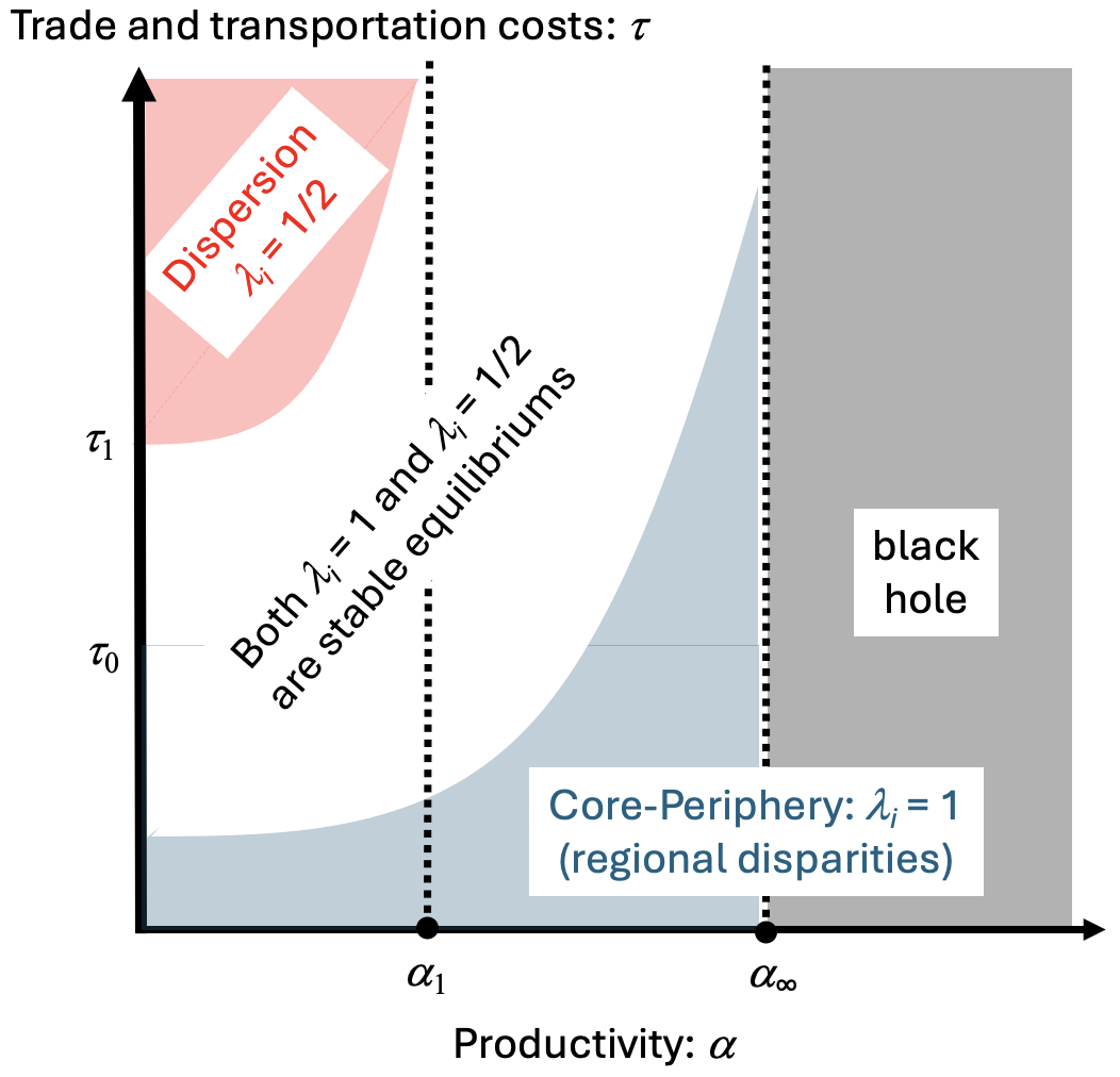
(a) Case $\sigma\in(1,2]$

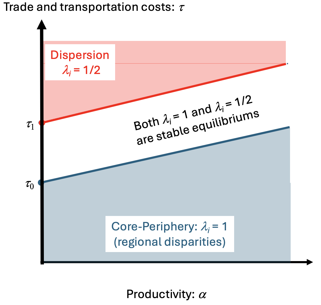
(b) Case $\sigma>2$

The Emergence of Black Holes.

Note that the core-periphery configuration emerges as the unique stable equilibrium for any level of trade costs $\tau>1$ if $\sigma\in\left(1,2\right]$ and $\alpha>\alpha_{\infty}\left(\sigma\right)$ because, in this case, agglomeration forces, as captured by the share of mobile expenditure $m^{B}$, always dominate dispersion forces, as captured by $\sigma-1$, and hence $m^{B}\geq\sigma-1$. Krugman (1991) refers to this case as a “black hole.” In his model, $m$ is a preference parameter and he rules out this case by imposing his famous “no black-hole condition”, as in this case his model fails to feature the richness of equilibrium configurations that the complementary parameter space provides. In our model, $m$ is an endogenous variable and the black hole configuration emerges as an equilibrium outcome when labor productivity is high enough. An important implication of this results is that prohibitive transportation costs in a sector are not inconsistent with its spatial clustering. Our model can thus accommodate the agglomeration of non-traded services as an equilibrium outcome.

Robustness to the Helpman Critique.

The qualitative results in this section are robust to Helpman’s critique of Krugman’s model (Helpman, 1998). In Krugman’s original model, the source of immobile demand is agriculture. This good produces under constant returns to labor and it is freely traded. Its price depends only on model parameters in equilibrium. Helpman (1998) points out the fragility of the result by reversing the model assumptions. He introduces housing as the source of immobile demand. Housing is among the most inherently non-tradable of services and its equilibrium return depends on the spatial distribution of economic activity. As a result, Helpman shows that in this alternative setting dispersion forces dominate agglomeration forces when inter-regional trade and transportation costs in manufacturing are low enough, turning this specific result of Krugman’s on its head. We show formally in Appendix D that our results are robust to Helpman’s criticism. We develop an extension of the model with a non-traded factor – structures – which yields a dispersion force that is independent of transportation costs in manufacturing. Thus, the symmetric equilibrium is stable for arbitrarily small levels of transportation costs in this alternative setting. Nevertheless, we show that the symmetric equilibrium is unstable for arbitrarily large levels of trade costs if $m>\sigma-1$, which is the exact same condition as in our current model.

6 Structural Change and Spatial Disparities

We are now ready to close the analysis of the interplay between structural change and the emergence of spatial disparities. Building on the tradition of the neoclassical growth model, we consider an economy in which growth is driven by exogenous labor-augmenting technical progress. As in Kongsamut, Rebelo, and Xie (2001), this uniform productivity growth drives the reallocation of labor from agriculture to manufacturing due to non-homothetic demand. For simplicity, there is no capital accumulation in our model, and different periods of time are a succession of static equilibriums. Given the spatial equilibrium configuration $j\in\left\{B,C\right\}$, the national (nominal) income is equal to

$$Y^{j}\left(\alpha,\sigma,\tau\right)\equiv w+\pi^{j}\left(\alpha,\sigma,\tau\right)=\alpha\left(1+\frac{1}{\sigma-m\left(\alpha,\sigma,\tau\right)}\right).$$ (28)

Per capita nominal income is equal to $\frac{Y}{2}$.The share of manufacturing in national income is equal to

$$\tilde{m}^{j}\left(\alpha,\sigma,\tau\right)\equiv\frac{\pi^{j}\left(\alpha,\sigma,\tau\right)}{\pi^{j}\left(\alpha,\sigma,\tau\right)+w}=\frac{1}{1+\sigma-m^{j}\left(\alpha,\sigma,\tau\right)},$$ (29)

and the earnings premium of entrepreneurs is equal to:

$$\tilde{\pi}^{j}\left(v\right)\equiv\frac{\pi^{j}\left(v\right)}{w}=\frac{1}{\sigma-m^{j}\left(\alpha,\sigma,\tau\right)}.$$ (30)

By inspection, all these variables are increasing in the manufacturing expenditure share $m$. Thus, labor-augmenting technical progress – modeled as a continuous increase of $\alpha$ over time – raises national and per-capita incomes (by equation 28), the share of manufacturing in the economy (by equation 29), and the earnings premium of entrepreneurs (by equation 30). Formally:

Proposition 14.

Growth and structural change. Assume labor productivity $\alpha$ increases over time. Then, given any spatial equilibrium $j\in\left\{B,C\right\}$, national income $Y$, per-capita income $\frac{Y}{2}$, the share of manufacturing $\tilde{m}$, and the earnings premium of entrepreneurs $\tilde{\pi}$ all increase over time.

Observe that the effect of productivity growth on structural change and earnings inequality is exclusively mediated through the manufacturing expenditure share $m$. That is, $m$ is increasing in labor productivity $\alpha$ because manufactures are a luxury good. By contrast, labor productivity has both a direct effect on income and an indirect effect through $m$. As we have extensively discussed in the previous section, technical progress also drives the spatial reallocation of manufacturing firms. To understand how our model brings together the notions of structural change and spatial disparities, it is useful to return to the abstract of the seminal Krugman (1991) paper:

This paper develops a simple model that shows how a country can endogenously become differentiated into an industrialized “core” and an agricultural “periphery.” In order to realize scale economies while minimizing transport costs, manufacturing firms tend to locate in the region with larger demand, but the location of demand itself depends on the distribution of manufacturing. Emergence of a core-periphery pattern depends on transportation costs, economies of scale, and the share of manufacturing in national income [p.483].

This abstract mentions three important drivers of regional disparities in the model. The first one is transportation costs ($\tau$ in the model). The typical comparative statics exercise of most contributions in the neg literature is to consider the consequences of a steady reduction of trade and transportation costs. This particular focus generated a lot of interest particularly in Europe. Summarizing this body of work, Puga (2002) concludes that the rise of regional disparities in Europe is a likely consequence of massive investments in transportation infrastructures and of the implementation of the Single Market Program. The second one is scale economies. In equilibrium, unexploited scale economies are increasing in product differentiation (decreasing in $\sigma$) by free-entry. The lower $\sigma$, the larger the equilibrium size of firms. A higher $\sigma$ also makes demand for individual varieties more sensitive to trade costs, as is captured by the combination of parameters, $\tau^{1-\sigma}$, that enters the equilibrium conditions. The final ingredient in Krugman’s abstract is the relative importance of the sector featuring scales economies – manufacturing – in the national economy. The larger it is, the stronger are self-reinforcing agglomeration economies, and the more likely regional disparities emerge in equilibrium. This share is a $parameter$ in Krugman’s core-periphery model. It is an endogenous $outcome$ in ours.

Consider, then, the following thought experiment. Assume that labor productivity is initially low, with $\alpha<\alpha_{1}$, and trade costs are initially high, with $\tau>\tau_{1}$, so that manufacturing is evenly dispersed across both regions at the unique stable equilibrium. Assume further that labor productivity monotonically increases over time, holding other parameters fixed (in particular $\tau$ and $\sigma$). Per capita incomes and economic well-being rise. In turn, the share of spending on manufacturing increases and that on agriculture falls. The first implication of this process is that labor reallocates from agriculture to manufacturing: structural change takes place (see proposition 14). As the share of spending on manufactures increases, a second implication is that agglomeration forces strengthen and dispersion forces weaken. Eventually, the spatial concentration of manufacturing becomes a possibility (as $\alpha$ rises above $\alpha_{1}$), and, then, from a possibility, it becomes the only stable equilibrium outcome (as $\alpha$ rises above $\alpha_{\infty}$): regional disparities emerge (see proposition 13).

This evolution is graphically depicted in Figure 3. As productivity grows over time and utility increases, the expenditure share in manufacturing rises. Eventually, the core-periphery equilibrium becomes possible since the sustain point is crossed. As productivity keeps growing, the core-periphery equilibrium is the only stable equilibrium and agglomeration of manufacturing at the core is a foregone conclusion.

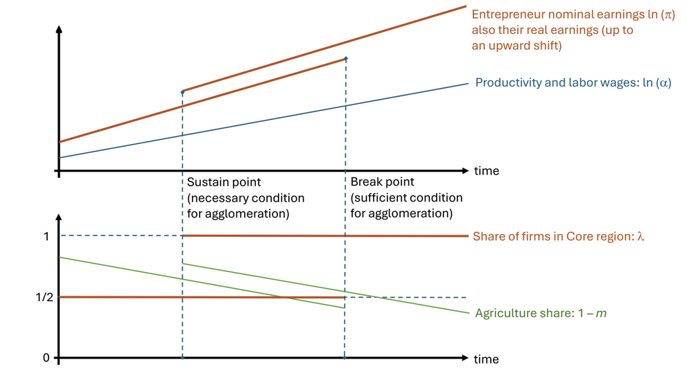
Figure 3: Dynamics of Spatial Structural Change

The relationship between regional disparities and structural change goes both ways. The emergence of regional disparities has a positive feedback effect on structural change because, as industry concentrates in a region, the economic well being of entrepreneurs increases, everything else equal, and with it their expenditure on manufacturing (see lemma 12). As a result, the national expenditure share in manufacturing further increases. This two-way interaction between agglomeration and structural change is absent from standard structural change models that abstract from the study of the spatial distribution of economic activity. Our model is stylized in that there are only two locations and only two potential stable equilibriums: symmetric or core-periphery. We believe that extending the model to more locations would magnify the importance of the two-way interaction we described, and we plan to study it in subsequent work.

Structural change brought about by the combination of the steady growth of labor productivity and of manufacturing being a luxury good also has an effect on individual income inequality. Though it benefits both types of factor owners, productivity growth disproportionately benefits the owners of the factor used intensively in the sector growing the most – entrepreneurs (see proposition 14). The logic is well-known since at least Jones (1965), and here it extends to the case of a factor specific to a monopolistically competitive sector. Summarizing:

Proposition 15.

Structural change and spatial disparities. Assume labor productivity $\alpha$ increases over time, all other things equal. Then, starting from an initially low value $\alpha<\alpha_{1}$, (i) structural change takes place: expenditure and employment are reallocated from agriculture to manufacturing; (ii) regional disparities may (if $\alpha_{1}<\alpha<\alpha_{\infty}$) and will (if $\alpha_{\infty}<\alpha$) emerge in equilibrium; (iii) regional disparities reinforce structural change; and (iv) structural change leads to an increase in the earnings premium of entrepreneurs.

7 Conclusion

In this paper, we develop a parsimonious model featuring non-homothetic demand to bring together the notions of structural change and regional disparities. To this aim, we introduce Heterothetic Cobb-Douglas preferences, which combine income effects with a unitary price elasticity of demand. This latter property keeps the model extremely tractable, and we expect it to be useful to applications in many other contexts. We incorporate a two-region neg model into a two-sector structural change framework. As labor productivity exogenously and monotonically increases over time, economic well-being rises and the expenditure share on agricultural goods falls. As a result, labor reallocates away from agriculture, and industry concentrates spatially: structural change and regional disparities are two outcomes of the growth process. Moreover, the industrial concentration increases productivity, which in turn leads to higher real incomes and a further reallocation away from agriculture. As such, structural change and regional disparities are also two mutually reinforcing propagators of the growth process.

The fundamental reason structural change strengthens self-enforcing agglomeration forces in the model (by increasing the share of mobile expenditure in the economy) is robust to the specific assumptions of Krugman’s core-periphery model (Krugman, 1991). By contrast, the role of trade and transportation costs on the rise and fall of regional disparities is highly sensitive to some modeling choices (Davis, 1998; Krugman and Venables, 1995; Puga, 1999). In Krugman’s original model, the source of immobile demand is agriculture. Helpman (1998) points out the fragility of the result by reversing the model assumptions. He introduces housing as the source of immobile demand. and shows that in this alternative setting dispersion forces dominate agglomeration forces when inter-regional trade and transportation costs in manufacturing are low enough, reversing Krugman’s original result.

By contrast, the chain of logic that we emphasize—from productivity growth to structural change and from structural change to regional disparities—works in both Krugman’s and Helpman’s cases. Specifically, it works under the assumption that the composite good combining manufacturing and services is a luxury and the other good, be it agriculture or housing, a necessity. Empirically, the income elasticity of demand for both agriculture (Herrendorf, Rogerson, and Valentinyi, 2014) and housing (Combes, Duranton, and Gobillon, 2019) is lower than one.

Our model is also amenable to extensions with more than two sectors since hcd preferences can accommodate any number of sectors and goods. In particular, we view studying the full transition from agriculture, to manufacturing, and to services as a promising avenue for studying structural changes and economic geography jointly. For a quantitative analysis, the model can be extended to multiple locations and non-unitary price effects can be introduced, e.g., through a nh-ces demand system. We anticipate that in both cases, the two-way interaction between structural change and agglomeration that we uncover may become more relevant as it triggers further structural change to services or to additional locations.

Appendix

Appendix A Proofs for Section 4

A.1 Lemma 3.

Lemma.

Regularity conditions. Assume preferences obey equation (9), and assume assumptions 1 and 2 hold; then in equilibrium (i) $C_{i}>\gamma$ and (ii) $\nicefrac{{\partial u}}{{\partial C_{i}}}>0$ for all $i\in I$.

Proof.

Part (i) is equivalent to showing that $C_{i}=\gamma$ implies the violation of the conditions imposed in 1, namely, that $P_{i}\gamma\geq\uline{s}y$. Minimizing total expenditure $\sum_{i}P_{i}C_{i}$ to reach an arbitrary level of utility $u>0$ yields the following first-order condition for $C_{i}$:

$$P_{i}-\frac{\theta\omega_{i}}{Ci}\geq 0,\quad C_{i}\geq\gamma,\quad\left(P_{i}-\frac{\theta\omega_{i}}{C_{i}}\right)\left(C_{i}-\gamma\right)=0,$$ (31)

where $\theta$ is the Lagrange multiplier associated with the constraint in equation (9). Thus, $C_{i}=\gamma$ requires $P_{i}\gamma\geq\theta\omega_{i}$, and we are set to showing $P_{i}\gamma\geq\theta\omega_{i}\Rightarrow P_{i}\gamma\geq\uline{s}y$ to establish part (i). Note first that $P_{i}\gamma<\uline{s}y$ for all $i\in{\cal N}$ implies that $y$ is above the level of expenditure required to cover the subsistence level

$$\sum_{i}P_{i}\gamma <\sum_{i}\uline{s}y<y,$$

where the second inequality follows from the fact that the sum of all goods minimum expenditure shares must be less than to the sum of their actual expenditure shares which sum to one. Thus, there exists a subset of goods $I_{+}\subseteq I$ such that $C_{j}>\gamma$ and $P_{j}C_{j}=\theta\omega_{j}$ for all $j\in I_{+}$. Denote the complementary subset of goods where $C_{i}=\gamma$ in equilibrium by $I_{-}$. We can then write:

$$y =\sum_{J\in I}P_{J}C_{J}$$

$$=\sum_{i\in I_{-}}P_{i}\gamma+\sum_{j\in I_{+}}P_{j}C_{j}$$

$$=\sum_{i\in I_{-}}P_{i}\gamma+\theta\sum_{j\in I_{+}}\omega_{j},$$

where the first equality equalizes income with expenditure, the second exploits the partition into goods consumed at the subsistence level and those consumed above it, and the third exploits the first order condition for the intensive margin of the latter category. Solving for $\theta$, we obtain:

$$\theta=\frac{y-\sum_{i\in I_{-}}P_{i}\gamma}{\sum_{j\in I_{+}}\omega_{j}}.$$

Plugging this expression into the first order condition for goods $i\in I_{-}$ yields:

$$P_{i}\gamma\geq\frac{y-\sum_{i\in I_{-}}P_{i}\gamma}{\sum_{j\in I_{+}}\omega_{j}}\omega_{i}.$$

Multiplying both sides by $\sum_{j\in I_{+}}\omega_{j}$ and summing over goods $i\in I_{-}$ yields:

$$\left(\sum_{j\in I_{+}}\omega_{j}\right)\sum_{i\in I_{-}}P_{i}\gamma\geq\left(\sum_{i\in I_{-}}\omega_{i}\right)\left(y-\sum_{i\in I_{-}}P_{i}\gamma\right),$$

which we may rewrite as

$$\left(\sum_{j\in I_{+}}\omega_{j}+\sum_{i\in I_{-}}\omega_{i}\right)\sum_{i\in I_{-}}Pi\gamma\geq\left(\sum_{i\in I_{-}}\omega_{i}\right)y.$$

Rearranging and simplifying, we obtain:

$$\sum_{i\in I_{-}}Pi\gamma\geq\sum_{i\in I_{-}}\frac{\omega_{i}}{\omega}y,$$

which implies

$$\exists i\in I_{-}:\quad P_{i}\gamma \geq\frac{\omega_{i}}{\omega}y>\uline{s}y,$$

where the second inequality follows from part (i) of 1. Thus, if the condition in part (iii) of (1) holds, then $C_{i}>\gamma$ for all $i\in I$. This step completes the proof for part (i).

Part (ii). Totally differentiating equation (9) and rearranging it yields

$$\left[\frac{1}{u}-\sum_{i}\omega_{i}^{\prime}\left(u\right)\ln\left(\frac{\omega(u)}{\omega_{i}(u)}\frac{C_{i}}{\gamma}\right)\right]\mathrm{d}u=\sum_{i}\omega_{i}\left(u\right)\mathrm{d}\ln C_{i}.$$

The term in brackets on the left-hand-side of the expression above is positive by $\omega_{i}^{\prime}<0$, $C_{i}>\gamma$, and $\omega_{i}(u)<\omega(u)$. Therefore, $u$ is increasing in $C_{i}$ by $\omega_{i}>0$. ∎

A.2 Lemma 4

Lemma.

Indirect utility function. Assume assumptions 2 and 1 hold. Then the indirect utility $V\left(\{P_{i}\},y\right)$ associated with the preferences in equation (9) can be written implicitly as the fixed point for $v$ of the following expression:

$$\ln v=\sum_{i}\omega_{i}\left(v\right)\ln\left(\frac{y}{\gamma P_{i}}\right)..$$

This fixed point exists and is unique. Furthermore, $V\left(\{P_{i}\},y\right)$ is increasing in $y$, decreasing in $P_{i}$ for all $i\in I$, and homogeneous of degree zero in its arguments (and hence $V$ is a proper indirect utility function).

Proof.

Totally differentiating equation (4) and rearranging yield:

$$\left[\frac{1}{v}-\sum_{i}\omega_{i}^{\prime}\left(v\right)\ln\left(\frac{y}{\gamma P_{i}}\right)\right]\mathrm{d}v=\omega\left(v\right)\mathrm{d}\ln y-\sum_{i}\omega_{i}\left(v\right)\mathrm{d}\ln P_{i}.$$

The term in brackets on the left-hand-side of the expression above is positive by assumption 1. Thus, $v$ is increasing in $y$ and decreasing in $P_{i}$ by $\omega_{i}>0$. ∎

A.3 Lemma 5

Lemma.

Expenditure function. Assume assumptions 2 and 1 hold. Then the expenditure function $E\left(u,P_{A},P_{M}\right)$ associated with the preferences in equation (9) can be written as:

$$\ln E\left(\{P_{i}\},u\right) =\ln\gamma+\frac{\ln u}{\omega\left(u\right)}+\sum_{i}\frac{\omega_{i}\left(u\right)}{\omega(u)}\mathrm{d}\ln P_{i}$$ (32)

The function $E$ is increasing in its arguments and it is homogeneous of degree one in prices (and hence is a proper expenditure function).

Proof.

The proof is analogous to the proofs to lemmas 3 and Lemma, and hence is omitted. ∎

A.4 Proposition 8

Proposition.

Engel curves and structural change. Assume assumption 6 holds. Then (i) manufactures are a luxury good and the agricultural good is a necessity, and (ii) the allocation of workers across sectors follows the expenditure shares. Hence $L_{M}$ is increasing in the level of utility $u$ in equilibrium.

Proof.

(i) Manufactures are a luxury good if and only if the income elasticity of demand is larger than one. With only two goods in the economy, this requirement is equivalent to saying that $m=\frac{\omega_{M}}{\omega_{A}+\omega_{M}}$ is increasing in $u$, which can happen if and only if $\frac{\omega_{M}}{\omega_{A}}$ is increasing in $u$. (ii) By inspection, $L_{M}$ is increasing in $m$, which is increasing in $u$ by part (i). ∎

A.5 Lemma 7

Lemma.

Sufficient regularity conditions. If parameter values are such that the following inequality holds:

$$\frac{\gamma\sigma\tau}{\uline{s}}<1,$$ (33)

then the sufficient condition in assumption 1 holds.

Proof.

Equation (14) implies $P_{M}\leq\tau$, and $P_{A}=1$ by equation (12). Turn to equation (16), and rewrite it as follows:

$$\sigma\pi^{r} =\frac{\lambda^{r}m\left(u^{r}\right)\pi^{r}+\frac{\alpha}{2}}{\lambda^{r}+\left(1-\lambda^{r}\right)\tau^{1-\sigma}}+\frac{\left(1-\lambda^{r}\right)m\left(u^{s}\right)\pi^{s}+\frac{\alpha}{2}}{\left(1-\lambda^{r}\right)\tau^{\sigma-1}+\lambda^{r}}$$

$$\geq\frac{\alpha}{2}\left[\frac{1}{\lambda^{r}+\left(1-\lambda^{r}\right)\tau^{1-\sigma}}+\frac{1}{\left(1-\lambda^{r}\right)\tau^{\sigma-1}+\lambda^{r}}\right].$$

From $\sigma,\tau>1$ and $0\leq\lambda^{r}\leq 1$, it follows that the term in the square bracket is larger than 2. Then, the earnings of an entrepreneur are larger than $\pi>\frac{\alpha}{\sigma}$, and in turn the right-hand side of expression (33) is a lower bound for the right-hand side of the inequality in assumption 1. Hence, if the former inequality holds, so does the latter. ∎

Appendix B Proofs for Section 5

B.1 Lemma 10

Lemma.

Sustain point. Let $\alpha_{1}\left(\sigma\right)>0$ be defined implicitly by $m\left(\alpha_{1},\sigma,1\right)=\sigma-1$ when $\sigma\in\left(1,2\right]$, with $\alpha_{1}^{\prime}>0$ by equation (21). (i) If $\sigma\in\left(1,2\right]$ and $0<\alpha\leq\alpha_{1}\left(\sigma\right)$, then $\Omega^{s}\leq\Omega^{C}$ if $\lambda^{r}=1$ for any value of $\tau$ in $\left[1,\tau_{1}\right]$. (ii) If $\sigma\in\left(1,2\right]$ and $\alpha>\alpha_{1}\left(\sigma\right)$, then $\Omega^{s}\leq\Omega^{C}$ if $\lambda^{r}=1$ for any $\tau\geq 1$. (iii) If $\sigma>2$, then $\Omega^{s}\leq\Omega^{CP}$ if $\lambda^{r}=1$ for any value of $\tau$ in $\left[1,\tau_{1}\right]$..

Proof.

Rewrite equation (24) as

$$f\left(\alpha,\sigma,\tau\right)\equiv 1-B_{1}\left(\alpha,\sigma\right)\tau^{b\left(\alpha,\sigma\right)}+B_{2}\left(\alpha,\sigma\right)\tau^{2\left(1-\sigma\right)}=0,\qquad B_{1},B_{2}>1.$$

By Descartes’s generalization of Laguerre’s rule of signs, this equation admits one positive root for $\tau$ if $b\left(\alpha,\sigma\right)>0$, as is in cases (i) and (iii) of the lemma, and it admits two positive roots if $b\left(\alpha,\sigma\right)<0$, as in case (ii). In the former case, it is easily verified by inspection of equation (24) that this root is $\tau=1$, and, from equations (20), (23), and (24), that $\Omega^{C}>\Omega^{s}$ whenever $\tau>1$. If instead $b\left(\alpha,\sigma\right)<0$, then we can establish with some algebra that $\lim_{\tau\rightarrow\infty}f\left(\alpha,\sigma,\tau\right)=0$, $\lim_{\tau\rightarrow 1}f\left(\alpha,\sigma,\tau\right)=-\infty$, $\lim_{\tau\rightarrow\infty}f^{\prime}\left(\alpha,\sigma,\tau\right)=+\infty$, and $\lim_{\tau\rightarrow 1}f^{\prime}\left(\alpha,\sigma,\tau\right)<0$, hence there exists a unique $\tau_{1}\in\left(1,\infty\right)$ such that $f\left(\alpha,\sigma,\tau_{1}\right)=0$. ∎

B.2 Lemma 11

Lemma.

Break point. Let $\alpha_{\infty}\left(\sigma\right)>0$ be defined implicitly by $m\left(\alpha_{\infty},\sigma,\infty\right)=\sigma-1$ when $\sigma\in\left(1,2\right]$, with $\alpha_{\infty}^{\prime}>0$ by equation (21). (i) If $\sigma\in\left(1,2\right]$ and $0<\alpha<\alpha_{\infty}\left(\sigma\right)$, then, the symmetric equilibrium is unstable for any value of $\tau$ in $\left[1,\tau_{0}\right]$. (ii) If $\sigma\in\left(1,2\right]$ and $\alpha>\alpha_{\infty}\left(\sigma\right)$, then the symmetric equilibrium is unstable for any $\tau\geq 1$. (iii) If $\sigma>2$, then the symmetric equilibrium is unstable for any value of $\tau$ in $\left[1,\tau_{0}\right]$.

Proof.

The formal analysis of the stability of the break point was initiated by Puga (1999) and is now standard; see e.g., Baldwin, Forslid, Martin, Ottaviano, and Robert-Nicoud (2003), Fujita, Krugman, and Venables (1999), or Robert-Nicoud (2005). Specifically, we totally differentiate equations (14), (16), and (17) around $\lambda^{r}=\lambda^{s}=\frac{1}{2}$, and to check for conditions under which $\frac{\partial\Omega^{r}}{\partial\lambda^{r}}<0$ at this symmetric equilibrium; the symmetric equilibrium is said to be stable under these conditions. If there exists a combination of parameters $\left(\alpha,\sigma,\tau\right)$ in the admissible range $\left(1,\infty\right)^{3}$ such that $\frac{\partial\Omega^{r}}{\partial\lambda^{r}}=0$, then this combination satisfies equation (26). The only difference between our model and the earlier literature is that expenditure share on manufactures, $m$, is an endogenous variable here while it is a parameter in the neg there. However, the break point is defined as the parameter configuration such that the change in utility following the move of an atomistic entrepreneur is exactly zero. Since the change in utility is zero, it follows from $m^{\prime}\left(\Omega\right)>0$ that $m$ is unchanged, too. The rest of the proof is similar to that of lemma 10, and hence is omitted here. ∎

B.3 Lemma 12

Lemma.

Equilibriums ranking. (i) Given parameter values $\left\{\alpha,\phi,\sigma\right\}$, the utility of entrepreneurs is strictly higher at the core-periphery equilibrium than at the symmetric equilibrium:

$$\forall\left\{\alpha,\sigma,\tau\right\}:\quad\Omega^{B}\left(\alpha,\sigma,\tau\right)<\Omega^{C}\left(\alpha,\sigma,1\right).$$ (34)

This result implies in turn $m^{B}<m^{C}$, and $\pi^{B}<\pi^{C}$. (ii) Given parameter values $\left\{\alpha,\sigma\right\}$, $\tau_{1}>\tau_{0}$. (iii) Any spatial equilibrium other than $\lambda\in\left\{0,\frac{1}{2},1\right\}$, if it exists at all, is not stable.

Proof.

(i) Note that $\Omega^{B}=\Omega^{C}$ if $\tau=1$. Thus, to show $\Omega^{B}<\Omega^{C}$ it suffices to show that $\Omega^{B}$ is continuously decreasing in $\tau$. Totally differentiating equation (25) yields

$$\mathrm{d}\ln\Omega^{B}-m^{B}\left[\frac{1}{\sigma-m^{B}}-\frac{1}{\sigma-1}\ln\left(\frac{2}{1+\tau^{1-\sigma}}\right)\right]\mathrm{d}\ln m^{B} =\mathrm{d}\ln\alpha-m^{B}\frac{\tau^{1-\sigma}}{1+\tau^{1-\sigma}}\mathrm{d}\ln\tau,$$

which we may rewrite as

$$\mathrm{d}\ln\Omega^{B}\left\{1-m^{B}\left[\frac{1}{\sigma-m^{B}}-\frac{1}{\sigma-1}\ln\left(\frac{2}{1+\tau^{1-\sigma}}\right)\right]\frac{\partial\ln m^{B}}{\partial\ln\Omega^{B}}\right\}=\mathrm{d}\ln\alpha-m^{B}\frac{\tau^{1-\sigma}}{1+\tau^{1-\sigma}}\mathrm{d}\ln\tau.$$ (35)

Consider the following term in the braces of the expression above:

$$m^{B}\left[\frac{1}{\sigma-m^{B}}-\frac{1}{\sigma-1}\ln\left(\frac{2}{1+\tau^{1-\sigma}}\right)\right] \leq\frac{1}{\sigma-1}-\frac{1}{\sigma-1}\ln\left(\frac{2}{1+\tau^{1-\sigma}}\right)$$

$$\leq\frac{1}{\sigma-1}.$$

Under assumption (9), then, the term inside braces in equation (35) is positive, and $\Omega^{B}$ is decreasing in $\tau$, and hence $\Omega^{B}<\Omega^{C}$, as was to be shown. (ii) Consider the break point in equation (25), and evaluate this expression for $m^{B}\left(\alpha,\sigma,\tau\right)=m^{C}$. Let

$$\left(\tilde{\tau}_{0}\right)^{1-\sigma}\equiv\frac{\sigma-1-m^{C}}{\sigma-1+m^{C}}\frac{\sigma-m^{C}}{\sigma+m^{C}},$$

which is the break point treating $m$ as a parameter, which we fix at $m^{C}.$ In this case, Robert-Nicoud (2005) shows that $\tilde{\tau}_{0}<\tau_{1}$ holds. Thus, we are left to showing that $\tau_{0}<\tilde{\tau}_{0}$ holds. To see that this is indeed the case, observe that it follows from $\Omega^{B}<\Omega^{C}$ and assumption 6 that $m^{B}$ is decreasing in $\tau$, and that $m^{B}<m^{C}$ holds. Since $\tilde{\tau}_{0}$ is increasing in $m$ by inspection of the expression above (recall $\sigma>1$), it follows that $\tau_{0}<\tilde{\tau}_{0}$ holds, and hence $\tau_{0}<\tau_{1}$ holds, as was to be shown. (iii) Robert-Nicoud (2005) shows that this result is a corollary to part (ii) of this lemma. ∎

B.4 Proposition 13

Proposition.

If $\sigma\in\left(1,2\right]$, then $\exists\alpha_{1}\left(\sigma\right),\alpha_{\infty}\left(\sigma\right)>0$ defined implicitly as $m^{C}\left(\alpha_{1},\sigma,1\right)=\sigma-1$ and $m^{B}\left(\alpha_{\infty},\sigma,\infty\right)$, respectively, with $0<\alpha_{1}\left(\sigma\right)<\alpha_{\infty}\left(\sigma\right)$. (i) The symmetric equilibrium is the unique stable equilibrium configuration in either of the following cases: if $\sigma>2$ and $\tau>\tau_{1}\left(\alpha,\sigma\right)$; or if $\sigma\in\left(1,2\right]$, $0<\alpha<\alpha_{1}\left(\sigma\right)$, and $\tau>\tau_{1}\left(\alpha,\sigma\right)$. (ii) The core-periphery configuration is the unique stable equilibrium in any of the following cases: if $\sigma>2$ and $\tau\leq\tau_{0}\left(\alpha,\sigma\right)$; if $\sigma\in\left(1,2\right]$, $0<\alpha<\alpha_{\infty}\left(\sigma\right)$, and $\tau\leq\tau_{0}\left(\alpha,\sigma\right)$; if $\sigma\in\left(1,2\right]$ and $\alpha\geq\alpha_{\infty}$$\left(\sigma\right)$. (iii) The symmetric equilibrium and the core-periphery pattern are both stable equilibrium configurations in any of the following cases: if $\sigma>2$ and $\tau_{0}\left(\alpha,\sigma\right)<\tau\leq\tau_{1}\left(\alpha,\sigma\right)$; or if $\sigma\in\left(1,2\right]$, $0<\alpha<\alpha_{1}\left(\sigma\right)$, and $\tau_{0}\left(\alpha,\sigma\right)<\tau\leq\tau_{1}\left(\alpha,\sigma\right)$; or if $\sigma\in\left(1,2\right]$, $\alpha_{1}\left(\sigma\right)<\alpha<\alpha_{\infty}\left(\sigma\right)$, and $\tau>\tau_{0}\left(\alpha,\sigma\right)$.

Proof.

The proof of this proposition is an immediate consequence of lemmas 10, 11, and 12. ∎

Appendix C Proofs for Section 6

C.1 Proposition Proposition

Proposition.

Growth and structural change. Assume labor productivity $\alpha$ increases over time. Then, given the spatial equilibrium $j\in\left\{B,CP\right\}$, national income $Y$, per-capita income $\frac{Y}{2}$, the share of manufacturing $\tilde{m}$, and the earnings premium of entrepreneurs $\tilde{\pi}$ all increase over time.

Proof.

By inspection of equations (28), (29), and (30). ∎

C.2 Proposition Proposition

Proposition.

Structural change and spatial disparities. Assume labor productivity $\alpha$ increases over time, all other things equal. Then, starting from an initially low value $\alpha<\alpha_{1}$, (i) structural change takes place: expenditure and employment are reallocated from agriculture to manufacturing; (ii) regional disparities may (if $\alpha_{1}<\alpha<\alpha_{0}$) and will (if $\alpha_{0}<\alpha$) emerge in equilibrium; (iii) regional disparities reinforce structural change; and (iv) structural change leads to an increase in the earnings premium of entrepreneurs.

Proof.

In the text above the proposition. ∎

Appendix D Encompassing Competition for Land

In the paper we assert that demand-driven structural change contributes to the emergence of regional disparities as long as the income elasticity of the demand for the combination of tradable services and manufacturing goods is larger than one (and the income elasticity of demand for agricultural goods is lower than one). Here we build a portmanteau model nesting both Krugman and Helpman’s mechanisms, of which the baseline model in our main text is a special case.

D.1 Model

We add structures to the in section 4. Specifically, we now have 3 sectors:

• Agriculture. This sector is like in section 4. It is competitive, it produces using labor only, and its output is freely traded.

• Manufacturing. As in section 4, entrepreneurs are the fixed factor. Now, the variable factor is a Cobb-Douglas combination of labor and structures, where $\eta\in\left[0,1\right]$ is Cobb Douglas share of structures. The model nests our Krugman-style model as a special case, with $\eta=0$, and a variant of Helpman’s model in the polar case $\eta=1$. Like in in section 4, this sector is monopolistically competitive and its output is traded at an iceberg cost $\tau$.

• Structures (factories). Structures are in fixed supply and are not traded. They are used in manufacturing production only (it is conceptually straightforward to also allow for housing consumption).

The main change with our baseline model is that we need impose the equilibrium condition for the market of structures:

$$\Lambda\rho^{r}=\eta\frac{\sigma-1}{\sigma}R^{r}=\eta\left(\sigma-1\right)\lambda^{r}\pi^{r}.$$ (36)

Above, $\rho^{r}$ is the equilibrium unit price of structures and $\Lambda$ is the fixed supply of land. We set $\Lambda=\eta\left(\sigma-1\right)$ by choice of units, thus $\rho^{r}=\lambda^{r}\pi^{r}$.

Manufacturing sales in equation (16) are now equal to

$$\sigma\pi^{r}=\left(\lambda^{r}\pi^{r}\right)^{\eta\left(1-\sigma\right)}\left\{\frac{E^{r}}{\Delta^{r}}+\tau^{1-\sigma}\frac{E^{s}}{\Delta^{s}}\right\},$$

where

$$E^{r}=\left[m\left(\Omega^{r}\right)+\eta\left(\sigma-1\right)\right]\lambda^{r}\pi^{r}+\frac{\alpha}{2}$$

denotes manufacturing expenditures, and

$$\Delta^{r}\equiv\left(P^{r}\right)^{1-\sigma}=\lambda^{r}\left(\lambda^{r}\pi^{r}\right)^{\eta\left(1-\sigma\right)}+\tau^{1-\sigma}\lambda^{s}\left(\lambda^{s}\pi^{s}\right)^{\eta\left(1-\sigma\right)}.$$

D.2 Hat Algebra

It proves useful to define $\hat{x}\equiv x^{r}/x^{s}$ for all $x=\lambda,\pi,\Delta,E,P$. Taking ratios of the expressions above yields:

$$\hat{\pi} =\left(\hat{\lambda}\hat{\pi}\right)^{\eta\left(1-\sigma\right)}\frac{\hat{E}+\tau^{1-\sigma}\hat{\Delta}}{\tau^{1-\sigma}\hat{E}+\hat{\Delta}}$$

$$\hat{E} =\frac{\alpha+\left[m^{r}+\eta\left(\sigma-1\right)\right]2\lambda^{r}\pi^{r}}{\alpha+\left[m^{s}+\eta\left(\sigma-1\right)\right]2\lambda^{s}\pi^{s}}$$

$$\hat{\Delta} =\frac{\hat{\lambda}^{1+\eta\left(1-\sigma\right)}\hat{\pi}^{\eta\left(1-\sigma\right)}+\tau^{1-\sigma}}{\tau^{1-\sigma}\hat{\lambda}^{1+\eta\left(1-\sigma\right)}\hat{\pi}^{\eta\left(1-\sigma\right)}+1}.$$ (37)

By the same token, if $m^{s}=m^{r}=m$, the ratio of real entrepreneur earnings is equal to

$$\hat{\Omega}=\hat{\pi}\hat{\Delta}^{\frac{m}{\sigma-1}}.$$

D.3 Stability of the Symmetric Equilibrium

At the symmetric equilibrium, $\hat{x}=1$ for all $x$, and $m^{r}=m^{s}=m$, some $m\in\left(0,1\right)$. In particular, the equilibrium earnings are equal to

$$\pi=\frac{\alpha}{\sigma-\left[m+\eta\left(\sigma-1\right)\right]},$$

which is positive by $\eta,m\in\left(0,1\right)$ and $\sigma>1$, and increasing in $m$. We are interested in the stability of this equilibrium. Let

$$Z\equiv\frac{1-\tau^{1-\sigma}}{1+\tau^{1-\sigma}}$$

be an index of trade frictions. By inspection, $Z$ is monotonically increasing in $\tau$ from $Z=0$ when $\tau=1$ (free trade) to $Z=1$ when $\tau\rightarrow\infty$ (autarky). Let also define the elasticity function as follows:

$${\cal E}\left(x\right)\equiv\left.\frac{\mathrm{d}\ln\hat{x}}{\mathrm{d}\ln\hat{\lambda}}\right|_{\hat{\lambda}=1}.$$

Using this compact notation, the symmetric equilibrium is said to be stable if

$${\cal E}\left(\Omega\right)={\cal E}\left(\pi\right)+\frac{m}{\sigma-1}{\cal E}\left(\Delta\right)$$ (38)

is negative, and unstable otherwise.

Differentiating the system in equation (37), we obtain

$${\cal E}\left(\pi\right) =-\eta\left(\sigma-1\right)\left[1+{\cal E}\left(\pi\right)\right]+Z\left[{\cal E}\left(E\right)-{\cal E}\left(\Delta\right)\right]$$

$${\cal E}\left(E\right) =2\tilde{m}\left[1+{\cal E}\left(\pi\right)\right]$$

$${\cal E}\left(\Delta\right) =Z\left\{1-\eta\left(\sigma-1\right)\left[1+{\cal E}\left(\pi\right)\right]\right\},$$

where

$$\tilde{m}\equiv\frac{m+\eta\left(\sigma-1\right)}{\sigma}$$

collects terms. By inspection, $\tilde{m}$ is increasing in $m$, and it belongs to the unit interval.

Let us rewrite the system of equations in matrix notation:

$$\left[\begin{array}[]{ccc}1+\eta\left(\sigma-1\right)&-Z&Z\\ -2\tilde{m}&1&0\\ -Z\eta\left(\sigma-1\right)&0&1\end{array}\right]\left[\begin{array}[]{c}{\cal E}\left(\pi\right)\\ {\cal E}\left(E\right)\\ {\cal E}\left(\Delta\right)\end{array}\right]=\left[\begin{array}[]{c}-\eta\left(\sigma-1\right)\\ 2\tilde{m}\\ Z\left[1-\eta\left(\sigma-1\right)\right]\end{array}\right].$$

Solving this system for ${\cal E}\left(\pi\right)$ and ${\cal E}\left(\Delta\right)$ and using equation (38) yields:

$${\cal E}\left(\Omega\right) =\frac{-\eta\left(\sigma-1\right)+2\tilde{m}Z-\left[1-\eta\left(\sigma-1\right)\right]Z^{2}+\frac{m}{\sigma-1}Z\left(1-2\tilde{m}Z\right)}{1-2\tilde{m}Z+\eta\left(\sigma-1\right)\left(1-Z^{2}\right)}$$

$$=\frac{-\eta\left(\sigma-1\right)\left(1-Z^{2}\right)+2\tilde{m}Z-Z^{2}+\frac{m}{\sigma-1}Z\left(1-2\tilde{m}Z\right)}{1-2\tilde{m}Z+\eta\left(\sigma-1\right)\left(1-Z^{2}\right)}$$

$$=-1+\frac{1-Z^{2}+\frac{m}{\sigma-1}Z\left(1-2\tilde{m}Z\right)}{1-2\tilde{m}Z+\eta\left(\sigma-1\right)\left(1-Z^{2}\right)}.$$ (39)

From the first line of equation (39), we obtain the following results:

1. The symmetric equilibrium is stable for arbitrarily low trade costs if $\eta>0$. Indeed,

   $$\left.{\cal E}\left(\Omega\right)\right|_{Z=0}=-\left(1+\frac{1}{\eta\left(\sigma-1\right)}\right)^{-1},$$

   which is unambiguously negative if $\eta>0$ (as in Helpman’s model) and zero if $\eta=0$ (as in Krugman’s model).

2. The symmetric equilibrium is unstable for arbitrarily high trade costs regardless of $\eta$ if expenditures on manufactures are high enough. Indeed,

   $$\left.{\cal E}\left(\Omega\right)\right|_{Z=1}=\frac{m}{\sigma-1}-1,$$

   which is positive if and only if $m>\sigma-1$ (as in Krugman’s model).

Appendix E Data Construction

We merge data from the Groningen 10 sector database, which we take from Comin et al. (2021), with the data from the urbanization rates from the United Nations Unhabitat Project. We drop from the resulting dataset Singapore and Hong Kong, since they are essentially city-states. The resulting dataset contains 37 countries, and spans from 1960 to 2010. The panel is not balanced though, the average number of years per country is 40.2, with a standard deviation of 9.1 years. The list of countries and the corresponding number of years with data follows: Argentina, 46 years of data; Bolivia, 44; Brazil, 12; Chile, 46; Colombia, 46; Costa Rica, 46; India, 35; Indonesia, 45; Japan, 44; Korea, 43; Mexico, 46; Malaysia, 31; Peru, 15; Philippines, 35; Thailand, 46; Venezuela, 44; West Germany, 24; Denmark, 36; Spain, 36; France, 36; Italy, 36; Netherlands, 36; Sweden, 36; USA, 46; UK, 46; Botswana, 43; Ethiopia, 50; Ghana, 31; Kenya, 42; Mauritius, 41; Malawi, 45; Nigeria, 51; Senegal, 41; Tanzania, 51; South Africa, 51; Zambia, 46.

References

- Baldwin et al. (2003) Richard Baldwin, Rikard Forslid, Philippe Martin, Gianmarco Ottaviano, and Frederic Robert-Nicoud. Economic Geography and Public Policy. Princeton University Press, 2003. ISBN 9780691123110. URL http://www.jstor.org/stable/j.ctt7skht.
- Baldwin et al. (2001) Richard E. Baldwin, Philippe Martin, and Gianmarco I. P. Ottaviano. Global income divergence, trade, and industrialization: The geography of growth take-offs. Journal of Economic Growth, 6(1):5–37, 2001. ISSN 13814338, 15737020. URL http://www.jstor.org/stable/40215903.
- Bohr et al. (2023a) Clement E Bohr, Marti Mestieri, and Frederic Robert-Nicoud. Heterothetic Cobb Douglas: Theory and Applications, 2023a. URL https://cepr.org/publications/dp18077.
- Bohr et al. (2023b) Clement E. Bohr, Marti Mestieri, and Emre Enes Yavuz. Engel’s treadmill: A theory of balanced growth and perpetual sectoral turnover, 2023b.
- Boppart (2014) Timo Boppart. Structural change and the Kaldor facts in a growth model with relative price effects and non-Gorman preferences. Econometrica, 82, 2014. ISSN 14680262. doi: 10.3982/ecta11354.
- Budi-Ors and Pijoan-Mas (2022) Thomas Budi-Ors and Josep Pijoan-Mas. Macroeconomic development, rural exodus, and uneven industrialization, 2022. URL https://cepr.org/publications/dp17086.
- Bustos et al. (2016) Paula Bustos, Bruno Caprettini, and Jacopo Ponticelli. Agricultural productivity and structural transformation: Evidence from brazil. American Economic Review, 106(6):1320–1365, June 2016. doi: 10.1257/aer.20131061. URL https://www.aeaweb.org/articles?id=10.1257/aer.20131061.
- Caselli and Coleman II (2001) Francesco Caselli and Wilbur John Coleman II. The u.s. structural transformation and regional convergence: A reinterpretation. Journal of Political Economy, 109(3):584–616, 2001. ISSN 00223808, 1537534X. URL http://www.jstor.org/stable/10.1086/321015.
- Charlot et al. (2006) Sylvie Charlot, Carl Gaigne, Frederic Robert-Nicoud, and Jacques Thisse. Agglomeration and welfare: The core-periphery model in the light of bentham, kaldor, and rawls. Journal of Public Economics, 90(1-2):325–347, 2006. URL https://EconPapers.repec.org/RePEc:eee:pubeco:v:90:y:2006:i:1-2:p:325-347.
- Chatterjee et al. (2024) Shoumitro Chatterjee, Elisa Giannone, Tatjana Kleineberg, and Kan Kuno. Unequal global convergence. 2024.
- Combes et al. (2019) Pierre-Philippe Combes, Gilles Duranton, and Laurent Gobillon. The Costs of Agglomeration: House and Land Prices in French Cities. The Review of Economic Studies, 86(4):1556–1589, July 2019. ISSN 0034-6527. doi: 10.1093/restud/rdy063.
- Comin et al. (2021) D. Comin, D. Lashkari, and M. Mestieri. Structural change with long-run income and price effects. Econometrica, 89, 2021. ISSN 14680262. doi: 10.3982/ECTA16317.
- Davis (1998) Donald R. Davis. The home market, trade, and industrial structure. The American Economic Review, 88(5):1264–1276, 1998. ISSN 00028282. URL http://www.jstor.org/stable/116870.
- Dennis and Iscan (2009) Benjamin N. Dennis and Talan Iscan. Engel versus baumol: Accounting for structural change using two centuries of u.s. data. Explorations in Economic History, 46(2):186–202, 2009. URL https://EconPapers.repec.org/RePEc:eee:exehis:v:46:y:2009:i:2:p:186-202.
- Desmet and Rossi-Hansberg (2014) Klaus Desmet and Esteban Rossi-Hansberg. Spatial development. American Economic Review, 104(4):1211–43, 2014.
- Dixit and Stiglitz (1977) Avinash K. Dixit and Joseph E. Stiglitz. Monopolistic competition and optimum product diversity. The American Economic Review, 67(3):297–308, 1977. ISSN 00028282. URL http://www.jstor.org/stable/1831401.
- Eckert and Peters (2022) Fabian Eckert and Michael Peters. Spatial structural change. Technical report, sep 2022.
- Faber (2014) Benjamin Faber. Trade integration, market size, and industrialization: Evidence from china’ s national trunk highway system. The Review of Economic Studies, 81(3):1046–1070, 2014. ISSN 0034-6527. doi: 10.1093/restud/rdu010.
- Fajgelbaum and Redding (2022) Pablo Fajgelbaum and Stephen J. Redding. Trade, structural transformation, and development: Evidence from argentina 1869-1914. Journal of Political Economy, 130(5):1249–1318, 2022. ISSN 1537-534X. doi: 10.1086/718915.
- Fally (2022) Thibault Fally. Generalized separability and integrability: Consumer demand with a price aggregator. Journal of Economic Theory, 203(C):S0022053122000618, 2022. URL https://EconPapers.repec.org/RePEc:eee:jetheo:v:203:y:2022:i:c:s0022053122000618.
- Finlay and Williams (2022) Robert Finlay and Trevor C. Williams. Sorting and the Skill Premium: The Role of Nonhomothetic Housing Demand. 2022.
- Forslid and Ottaviano (2003) Rikard Forslid and Gianmarco I.P. Ottaviano. An analytically solvable core-periphery model. Journal of Economic Geography, 3(3):229–240, 2003. doi: 10.1093/jeg/3.3.229.
- Fujita et al. (1999) Masahisa Fujita, Paul Krugman, and Anthony J. Venables. The Spatial Economy: Cities, Regions, and International Trade. The MIT Press, 1999. ISBN 9780262273329. doi: 10.7551/mitpress/6389.001.0001.
- Geary (1950) Roy C. Geary. A note on ’a constant-utility index of the cost of living’. Review of Economic Studies, 18(2):65–66, 1950.
- Gorman (1995) W. M. Gorman. Collected works of WM Gorman: Separability and aggregation. 1, 1995.
- Helpman (1998) Elhanan Helpman. The size of regions. In David Pines, Efraim Sadka, and Itzhak Zilcha, editors, Topics in Public Economics: Theoretical and Applied Analysis, pages 33–54. Cambridge University Press, Cambridge, 1998.
- Herrendorf et al. (2013) Berthold Herrendorf, Richard Rogerson, and Akos Valentinyi. Two perspectives on preferences and structural transformation. American Economic Review, 103(7):2752–2789, 2013. ISSN 0002-8282. doi: 10.1257/aer.103.7.2752.
- Herrendorf et al. (2014) Berthold Herrendorf, Richard Rogerson, and Akos Valentinyi. Growth and Structural Transformation, pages 855–941. Elsevier, 2014. doi: 10.1016/b978-0-444-53540-5.00006-9.
- Jones (1965) Ronald W. Jones. The structure of simple general equilibrium models. Journal of Political Economy, 73(6):557–572, 1965. ISSN 00223808, 1537534X. URL http://www.jstor.org/stable/1829883.
- Kongsamut et al. (2001) Piyabha Kongsamut, Sergio Rebelo, and Danyang Xie. Beyond balanced growth. The Review of Economic Studies, 68:869–882, 10 2001. ISSN 0034-6527. doi: 10.1111/1467-937X.00193. URL https://academic.oup.com/restud/article/68/4/869/1577689.
- Krugman and Venables (1995) P. Krugman and A. J. Venables. Globalization and the inequality of nations. The Quarterly Journal of Economics, 110(4):857–880, 1995. ISSN 1531-4650. doi: 10.2307/2946642.
- Krugman (1991) Paul Krugman. Increasing returns and economic geography. Journal of Political Economy, 99:483–499, 1991. ISSN 00223808. doi: 10.1086/261763. URL https://www.jstor.org/stable/2937739.
- Matsuyama (2016) Kiminor Matsuyama. The generalized engel’s law: In search for a new framework, 2016.
- Michaels et al. (2012) Guy Michaels, Ferdinand Rauch, and Stephen J. Redding. Urbanization and structural transformation. The Quarterly Journal of Economics, 127(2):535–586, 2012. ISSN 00335533, 15314650. URL http://www.jstor.org/stable/23251993.
- Mossay (2006) Pascal Mossay. The core-periphery model: A note on the existence and uniqueness of short-run equilibrium. Journal of Urban Economics, 59(3):389–393, 2006. ISSN 0094-1190. doi: 10.1016/j.jue.2005.10.007.
- Murata (2008) Yasusada Murata. Engel’s law, petty’s law, and agglomeration. Journal of Development Economics, 87(1):161–177, 2008. ISSN 0304-3878. doi: 10.1016/j.jdeveco.2007.06.001.
- Nagy (2023) David Krisztian Nagy. Hinterlands, city formation and growth: Evidence from the u.s. westward expansion. Review of Economic Studies, 90(6):3238–3281, 2023. ISSN 1467-937X. doi: 10.1093/restud/rdad008.
- Ottaviano et al. (2002) Gianmarco Ottaviano, Takatoshi Tabuchi, and Jacques-Francois Thisse. Agglomeration and trade revisited. International Economic Review, 43(2):409–435, 2002. ISSN 00206598, 14682354. URL http://www.jstor.org/stable/826994.
- Pfluger (2004) Michael Pfluger. A simple, analytically solvable, chamberlinian agglomeration model. Regional Science and Urban Economics, 34(5):565–573, 2004. ISSN 0166-0462. doi: 10.1016/s0166-0462(03)00043-7.
- Pollak (1972) Robert A. Pollak. Generalized separability. Econometrica, 40(3):431, 1972. ISSN 0012-9682. doi: 10.2307/1913177.
- Puga (2002) D. Puga. European regional policies in light of recent location theories. Journal of Economic Geography, 2(4):373–406, 2002. ISSN 1468-2710. doi: 10.1093/jeg/2.4.373.
- Puga (1999) Diego Puga. The rise and fall of regional inequalities. European Economic Review, 43(2):303–334, 1999. ISSN 0014-2921. doi: 10.1016/s0014-2921(98)00061-0.
- Puga and Venables (1996) Diego Puga and Anthony J. Venables. The spread of industry: Spatial agglomeration in economic development. Journal of the Japanese and International Economies, 10(4):440–464, 1996. ISSN 0889-1583. doi: 10.1006/jjie.1996.0025.
- Robert-Nicoud (2005) Frederic Robert-Nicoud. The structure of simple new economic geography models (or, on identical twins). Journal of Economic Geography, 5(2):201–234, 2005. doi: 10.1093/jnlecg/lbh037.
- Samuelson (1954) Paul A. Samuelson. The Transfer Problem and Transport Costs, II: Analysis of Effects of Trade Impediments. The Economic Journal, 64(254):264–289, 06 1954. ISSN 0013-0133. doi: 10.2307/2226834. URL https://doi.org/10.2307/2226834.
- Stone (1954) Richard Stone. Linear expenditure systems and demand analysis: An application to the pattern of british demand. Economic Journal, 64(255):511–527, 1954.
- Takeda (2022) Kohei Takeda. The geography of structural transformation: Effects on inequality and mobility. CEP Discussion Papers dp1893, Centre for Economic Performance, LSE, December 2022. URL https://ideas.repec.org/p/cep/cepdps/dp1893.html.