A Hybrid Deep-Learning Model for El Niño Southern Oscillation in the Low-Data Regime
Abstract
While deep-learning models have demonstrated skillful El Niño Southern Oscillation (ENSO) forecasts up to one year in advance, they are predominantly trained on climate model simulations that provide thousands of years of training data at the expense of introducing climate model biases. Simpler Linear Inverse Models (LIMs) trained on the much shorter observational record also make skillful ENSO predictions but do not capture predictable nonlinear processes. This motivates a hybrid approach, combining the LIM’s modest data needs with a deep-learning non-Markovian correction of the LIM. For O(100 yr) datasets, our resulting Hybrid model is more skillful than the LIM while also exceeding the skill of a full deep-learning model. Additionally, while the most predictable ENSO events are still identified in advance by the LIM, they are better predicted by the Hybrid model, especially in the western tropical Pacific for leads beyond about 9 months, by capturing the subsequent asymmetric (warm versus cold phases) evolution of ENSO.
1 Introduction
In the past few years, deep learning has revolutionized weather forecasting with models such as GraphCast (Lam et al., 2023), Pangu (Bi et al., 2023), and others (Pathak et al., 2022; Lang et al., 2024) now outperforming traditional state-of-the-art numerical weather prediction models (Ben-Bouallegue et al., 2023). These advancements are largely due to the availability of millions of training data samples from reanalysis products on hourly resolution, which allows the training of large neural networks with negligible generalization error. While these models demonstrate exceptional medium-range forecasting skill, it remains unclear if these capabilities extend to seasonal or annual predictions. Unlike medium-range forecasting, which is mainly dependent on initial conditions, long-range predictions are primarily determined by boundary forcing factors, particularly from the ocean.
A prominent example of a target for seasonal to annual forecasting is El Niño-Southern Oscillation (ENSO). Characterized by tropical Pacific sea surface temperature anomalies (SSTA), the ENSO strongly influences global weather patterns and is therefore a primary source of seasonal to annual predictability. Its events are characterized by anomalously warm (cold) tropical SSTA, which exhibit a rich diversity in their spatial structure, temporal evolution (Capotondi et al., 2015; Timmermann et al., 2018), and impact on extreme weather conditions worldwide (Taschetto et al., 2020; Strnad et al., 2022). Thus, early forecasts of the likelihood of an ENSO event and also of its expected spatial structure are of great value for sectoral applications worldwide (Callahan and Mankin, 2023).
While deep learning models have demonstrated their capacity for producing skillful ENSO forecasts (Ham et al., 2019; Petersik and Dijkstra, 2020; Cachay et al., 2021; Zhou and Zhang, 2023), training these models directly from SSTA data is hampered by the short observational record. Global SST records from satellites have been available for the past 40 years, with reconstructions based on point observations extending 100 years prior. In fact, Wittenberg (2009) suggested that O(500) years of data might be required to entirely capture the diversity of interannual ENSO events. Instead, deep learning models have been trained on lengthy simulations made by global circulation models (GCMs) (Ham et al., 2019; Zhou and Zhang, 2023), such as those available from the CMIP5 or CMIP6 ensembles. While potentially providing hundreds to thousands of years of data, GCM simulations possess inherent biases likely due to their insufficient spatial resolution and to inadequate parametrizations of unresolved processes. In the Tropical Pacific, such biases typically include mean errors in the equatorial upwelling region in the eastern Pacific and variability errors in the strength and location of ENSO anomalies (Capotondi, 2013; Chen et al., 2021; Beverley et al., 2023), all of which may then be captured by the neural network. Transfer learning, as for instance used by Ham et al. (2019), presents a potential workaround for bridging the gap between erroneous simulation data and limited observations. However, Zhou and Zhang (Zhou and Zhang, 2023) found no significant improvement in model performance when fine-tuning their model with reanalysis data, indicating the need for more research in this domain.
The Linear Inverse Model (LIM), first introduced by Penland and Sardeshmukh (1995), offers an alternative data-driven approach for ENSO forecasting. The LIM is a stochastic climate model (Hasselmann, 1976) that represents chaotic nonlinear dynamics by a deterministic multivariate linear system driven by noise that is white in time but may be correlated in space. This approximation may be suitable for dynamical systems with different components evolving on very different time scales, such as when the slowly-varying ocean is driven by and coupled to a much more rapidly decorrelating atmosphere (Frankignoul and Hasselmann, 1977; Penland, 1996). Even when determined from anomaly covariances drawn from the short observational record alone, the LIM demonstrates seasonal-to-interannual tropical SSTA forecast skill on par with operational numerical prediction models (Newman and Sardeshmukh, 2017; L’Heureux et al., 2020). Refinements to the LIM, such as the cyclostationary (CS)-LIM to account for the annual cycle (Shin et al., 2021; Vimont et al., 2022) and the inclusion of ocean memory (Newman et al., 2011; Chen et al., 2016), can further improve its predictive skill.
The LIM generates climate variability that has a multivariate Gaussian distribution. The tropical Pacific SSTA distribution, however, is non-Gaussian and asymmetric, with warm events being more intense than cold events, while cold events are typically of longer duration (Takahashi et al., 2011; Takahashi and Dewitte, 2016; Okumura, 2019; Geng and Jin, 2022). As a correction to the LIM, we might first try modifying its stochastic forcing to include a linearly state-dependent noise term that is correlated with the original state-independent noise (Sardeshmukh and Penland, 2015), the details of which in principle might also be extracted from observations (Martinez-Villalobos et al., 2018). Then, while the LIM’s predictable dynamics would remain linear, this additional “correlated additive-multiplicative” (CAM) noise term (Sardeshmukh et al., 2015) would drive non-Gaussian variability including some key aspects of the observed asymmetry in the intensity and duration of ENSO events (Martinez-Villalobos et al., 2019). However, ENSO asymmetry has also been attributed to slower nonlinear processes in the tropical Pacific (Dommenget et al., 2013; Takahashi et al., 2011, 2019; Hayashi et al., 2020), which might not be simply represented by CAM noise. Given that the LIM already shows substantial predictive skill, then, we could systematically investigate its forecast error residual for predictable nonlinear dynamics, and add the resulting correction of the LIM. Developing such a hybrid LIM model is our aim in this study.
Hybrid models, which combine numerical or empirical models with neural networks, offer a promising approach to capture unresolved dynamics in the low-data regime (Irrgang et al., 2021). Instead of learning the complex system dynamics of the full system with a neural network, hybrid approaches are often more data efficient due to their simpler learning objective. Applications include post-processing of weather forecasts (Gneiting et al., 2005; Bauer et al., 2015) and machine learning parametrization in coupled ocean-atmosphere models (Rasp and Lerch, 2018; Watt-Meyer et al., 2021; Kochkov et al., 2023).
In the context of ENSO forecasting, Goel et al. (2017) and others (Wang et al., 2021; Zhou and Zhang, 2022) combined RNNs with statistical models for forecasting Niño indices. Expanding beyond ENSO index prediction, Rodrigues et al. (2021) developed a hybrid model using the LIM operator within a ResNet-like architecture for global SSTA prediction. These hybrid approaches have not yet achieved state-of-the-art forecasting skill, and their potential advantages over fully deep learning models, such as interpretability and data efficiency, remain unexplored.
Here, we propose a hybrid deep-learning model for ENSO forecasting that combines the LIM with a Long-Short Term Memory (LSTM) network (Hochreiter and Schmidhuber, 1997). This LIM-LSTM hybrid model is designed to capture the residuals between LIM forecasts and target data, thereby improving seasonal forecast accuracy. We diverge from existing methodologies by including seasonality in both the LIM and the LSTM. Furthermore, we adapt both the hybrid model and the LSTM to generate probabilistic ensemble forecasts of the full field variables, SSTA and SSHA. This is achieved by employing a set of output layers that generate ensemble members, designed to match the nonparametric distribution of the target data (Lessig et al., 2023). We conduct a comparative analysis between our LIM-LSTM hybrid model and our LSTM deep-learning model, focusing on how each captures ENSO dynamics.
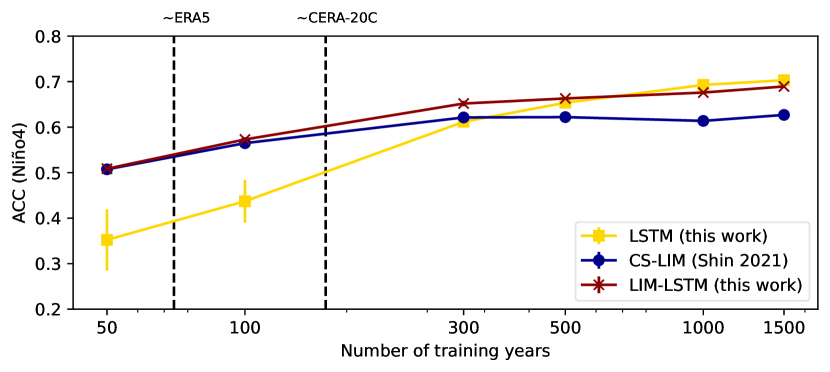
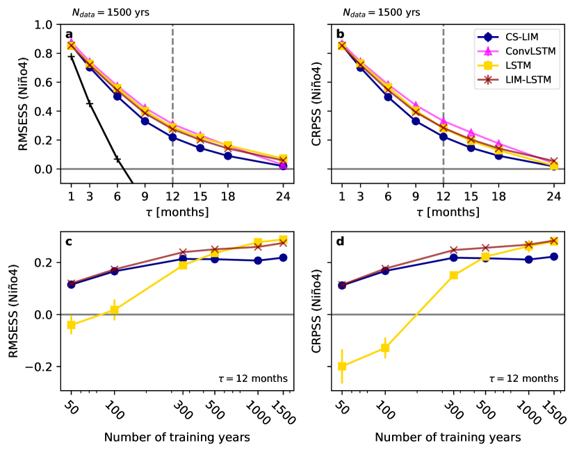
One key question we address in this study is the training data requirements needed for each technique to achieve a given level of ENSO prediction skill. Therefore, we develop the technique on a large model dataset. While this has limitations, it allows us to compare the data requirements for both our hybrid and full DL models by evaluating their skill on subsets of the data with varying lengths. As an example, Fig. 1 shows that for training on 50-100 years of monthly data, comparable in length to reanalysis products like ERA5 and CERA-20C, the 12-month forecast of both the CS-LIM and the LIM-LSTM hybrid model exhibit an Anomaly Correlation Coefficient (ACC) of bigger than 0.5 (the typical threshold for a forecast to be considered skillful). In contrast, for the same amount of training data, the 12-month forecast of the pure LSTM model’s has an ACC lower than 0.4, both evaluated on the 200-year long test set. It takes 300 years of data before the LSTM model reaches a forecast skill on par with the CS-LIM and LIM-LSTM hybrid model. Only when the training dataset size exceeds 500 years do both the LSTM and the LIM-LSTM model surpass the CS-LIM, with skillful forecasts (ACC > 0.5) up to leads of 18 months.
2 Results
2.1 Improved forecast skill due to predictable nonlinearities
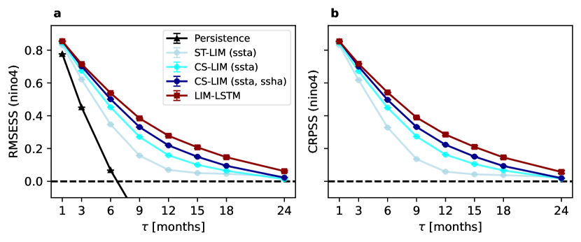
The CS-LIM estimated from the PCs of SSTA and SSHA of the first 1500 years of a CESM2 pre-industrial simulation in the tropical Pacific (see Methods sec. 4.1) captures the predictable linear dynamics of the system. We then trained an LSTM to learn the residuals between the CS-LIM’s predictions and the target data and combined these to form our hybrid LIM-LSTM model (see Methods sec. 4.5). Improved forecast skill of the LIM-LSTM, relative to the LIM itself, can thus be attributed to its ability to capture predictable nonlinearities of the tropical Pacific Ocean dynamics. We quantified this improvement in skill by computing deterministic and probabilistic skill scores (RMSE and CRPS; see Methods sec. 4.8) of the CS-LIM and LIM-LSTM on the test data (year 1800 to 2000). Both skill scores are obtained with respect to monthly climatology as a baseline model.
First, we would like to capture as much of the linear dynamics in the LIM as possible, so that the LSTM is primarily tasked with learning nonlinear dynamics from the LIM errors. Various LIM variants, with increasing levels of complexity, are constructed to guide the choice of the best linear model. The initial LIM variant, formulated by Penland and Sardeshmukh (1995), is solely fitted to the first 30 PCs of SSTA in the Pacific and is termed stationary (ST)-LIM (ssta). An advancement to this is the CS-LIM (ssta), introduced by Shin et al. (2021), which includes seasonal variations and substantially surpasses the skill of the ST-LIM (ssta), as shown by the RMSE (Fig. 2a) and CRPS (Fig. 2b) skill scores of the Niño4 index. For reference, we present the skill of the persistence forecast which is worse than a climatological forecast (dashed line at zero) after =6 months forecast lead time. Including a measure of ocean memory, by incorporating the first 10 PCs of SSHA in the tropical Pacific in the CS-LIM (ssta, ssha), leads to additional skill enhancement relative to the CS-LIM (ssta). We select SSHA for its availability in both model and observations, and for its strong relationship with important ENSO precursors, namely the upper ocean heat content and thermocline depth, following previous LIM studies (Johnson, 2001; Newman et al., 2011). Progressive improvements are evident in each LIM version, with the inclusion of seasonality and subsurface ocean variables contributing significantly to enhanced skill (Fig. 2). The CS-LIM (ssta, ssha) (CS-LIM hereafter) has the highest skill among the linear models and thus is considered the best representation of the predictable linear dynamics.
Our hybrid LIM-LSTM model builds upon the CS-LIM by using an LSTM that learns to correct the error between the LIM forecast and the target data. The LSTM takes 16 ensemble member forecasts of the CS-LIM as input and learns to model their residual errors to the target data by minimizing the CRPS loss function detailed in Eq. LABEL:eq:crps-loss. To ensure robustness, we repeat the model training five times with varied weight initialization and data shuffling, whose variability is depicted through error bars in Fig. 2. The skill improvement of the LIM-LSTM upon the CS-LIM is significant at forecast lead times larger than 6 months. We anticipate that the skill improvements can be largely attributed to predictable nonlinearities to the extent that we have tried to ensure that all known linear dynamics are captured by the CS-LIM.
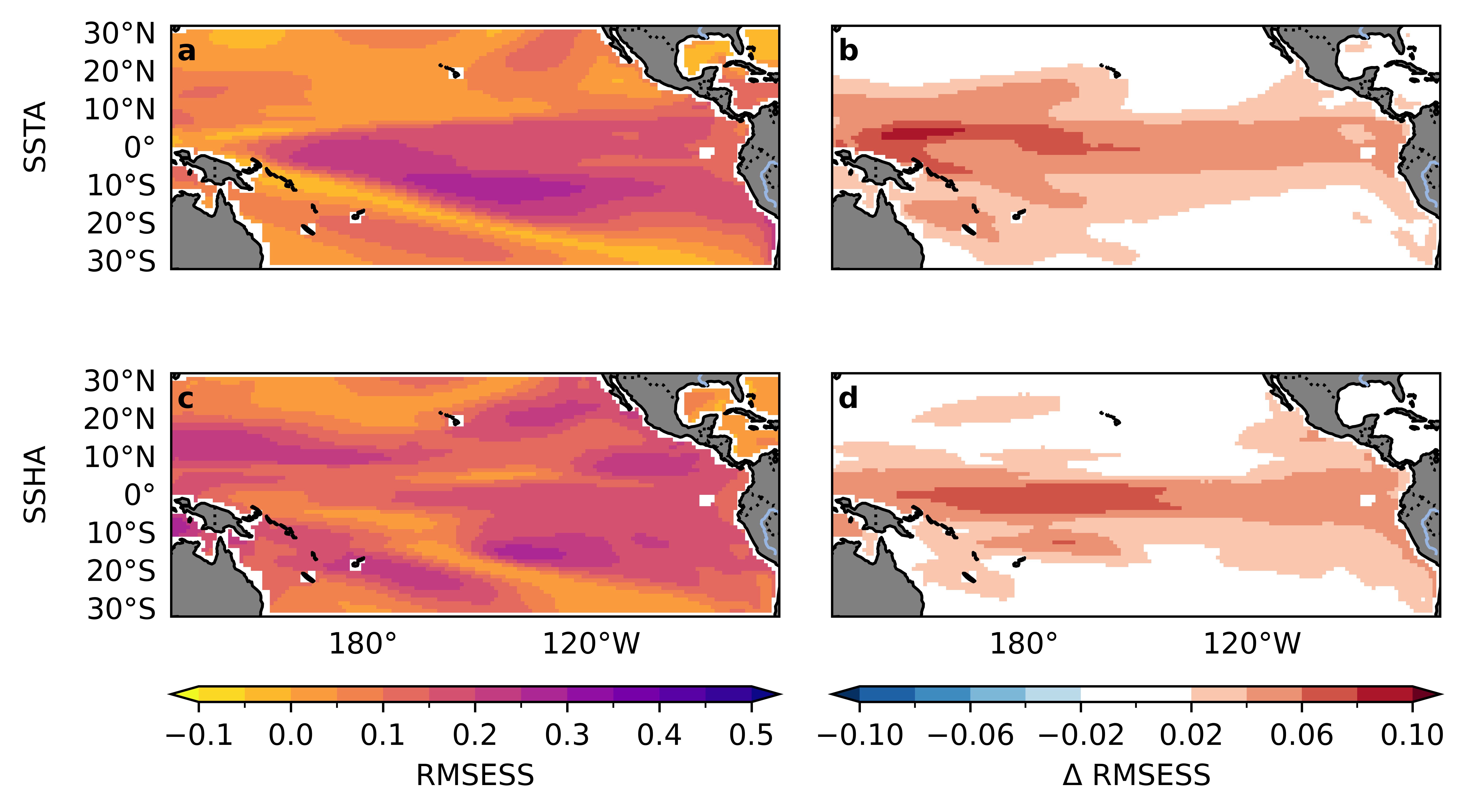
We conducted a further examination of the seasonal dependency (Sec. A.1) and spatial distribution of skill for both the LIM and the LIM-LSTM model. The ensemble mean RMSESS for a 12-month CS-LIM forecast of SSTA exhibits the highest skill south of the equator and the Niño4 region while the skill is notably smaller in the upwelling region in the eastern tropical Pacific (Fig. 3a). In contrast, the RMSESS of SSHA demonstrated high skill in this region as well as in western tropical Pacific north of the equator (Fig. 3c) where the largest centers of SSH variability associated with ENSO occur (Capotondi et al., 2020).
The LIM-LSTM improves upon the CS-LIM skill throughout the Tropics (Fig. 3b, d). There is a discernible skill improvement all along the equator, with the most significant enhancement observed in the western tropical Pacific. This improvement is consistent with the patterns obtained using the CRPSS (not shown). The pattern of skill improvement is different from the pattern of CS-LIM skill; that is, the LIM-LSTM often has less improvement in regions where the CS-LIM already shows substantial skill. It is interesting to note that the western warm pool shows the highest skill improvement, and also exhibits the warmest temperatures in the Pacific where the nonlinear ocean-atmosphere feedback is the largest (Thual and Dewitte, 2023). CESM2 and other climate models overestimate the SSTA variability in this region compared to observations which could increase this effect (Capotondi et al., 2020). We defer a detailed analysis of nonlinear drivers learned by the LSTM to a future study.
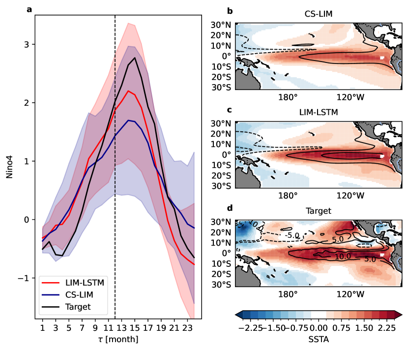
While both the LIM and LIM-LSTM can predict large El Niño events, the LIM-LSTM better captures event amplitudes. As an example, Fig. 4 shows 24-month forecasts made by both models for a chosen El Niño exemplar drawn from the test dataset. The forecasts are initialized in December, 12 months before the peak of the chosen El Niño event (dashed line in Fig. 4A). Throughout this work, we show the Niño4 instead of the Niño3.4 region because of the CESM2 tendency to achieve the largest ENSO SST anomalies in the central Pacific rather than the eastern Pacific (Capotondi et al., 2020). Results for the Niño3.4 index are qualitatively similar. Both the CS-LIM (red line) and LIM-LSTM (blue line) forecasts predict the observed warming, as depicted by the ensemble members’ mean, with the shading indicating their respective ensemble standard deviations. Notably, the LIM-LSTM forecast magnitude is closer to the CESM2 target data than the CS-LIM forecast. The LIM-LSTM’s uncertainty range, given by the standard deviation between 16 ensemble member forecasts, is also narrower than that of the CS-LIM forecast, yet still encompasses the target data, possibly suggesting a more accurate ensemble spread, consistent with the CRPSS results in Fig. 2. The SSTA and SSHA field forecasts at =12 months lead time (Fig. 4C, D) show that the LIM-LSTM generally better captures this El Niño event’s magnitude throughout the equatorial Pacific. However, both the CS-LIM and LIM-LSTM lack some smaller spatial structures and extratropical features evident in the verification fields.
2.2 Comparison to deep learning baselines
We conducted a comparative analysis between our hybrid LIM-LSTM and two fully deep learning models, the LSTM and the ConvLSTM (see Methods Sec. 4). While the LSTM produces forecasts in the PC space of SSTA and SSHA, the ConvLSTM takes the field variables in the tropical Pacific as input and forecasts them directly. We employ both models to ensure that the EOF truncation does not substantially hamper our forecast skill. Similar to the training of the LIM-LSTM, each model underwent five separate training sessions with varied weight initialization and data shuffling (error bars in Fig. 5). The deep learning models have RMSE and CPRS skill scores that are similar to the LIM-LSTM model (Fig. 5a, b), though the ConvLSTM exhibits a slight improvement at the 12-month forecast horizon. This suggests that the LIM-LSTM model successfully captures most of the predictable dynamics, with the marginal gains of the ConvLSTM likely attributable to the PC truncation of our hybrid model. Crucially, the LIM-LSTM model achieves this level of forecasting skill with significantly fewer parameters compared to the full deep learning models. This aspect is particularly beneficial in scenarios with limited data, as shown in Fig. 5c and d. With less than 500 years of monthly data, both the LIM and LIM-LSTM exhibit higher 12-month RMSES and CRPS skill scores than the LSTM.
2.3 Predictability assessment in the LIM-LSTM model
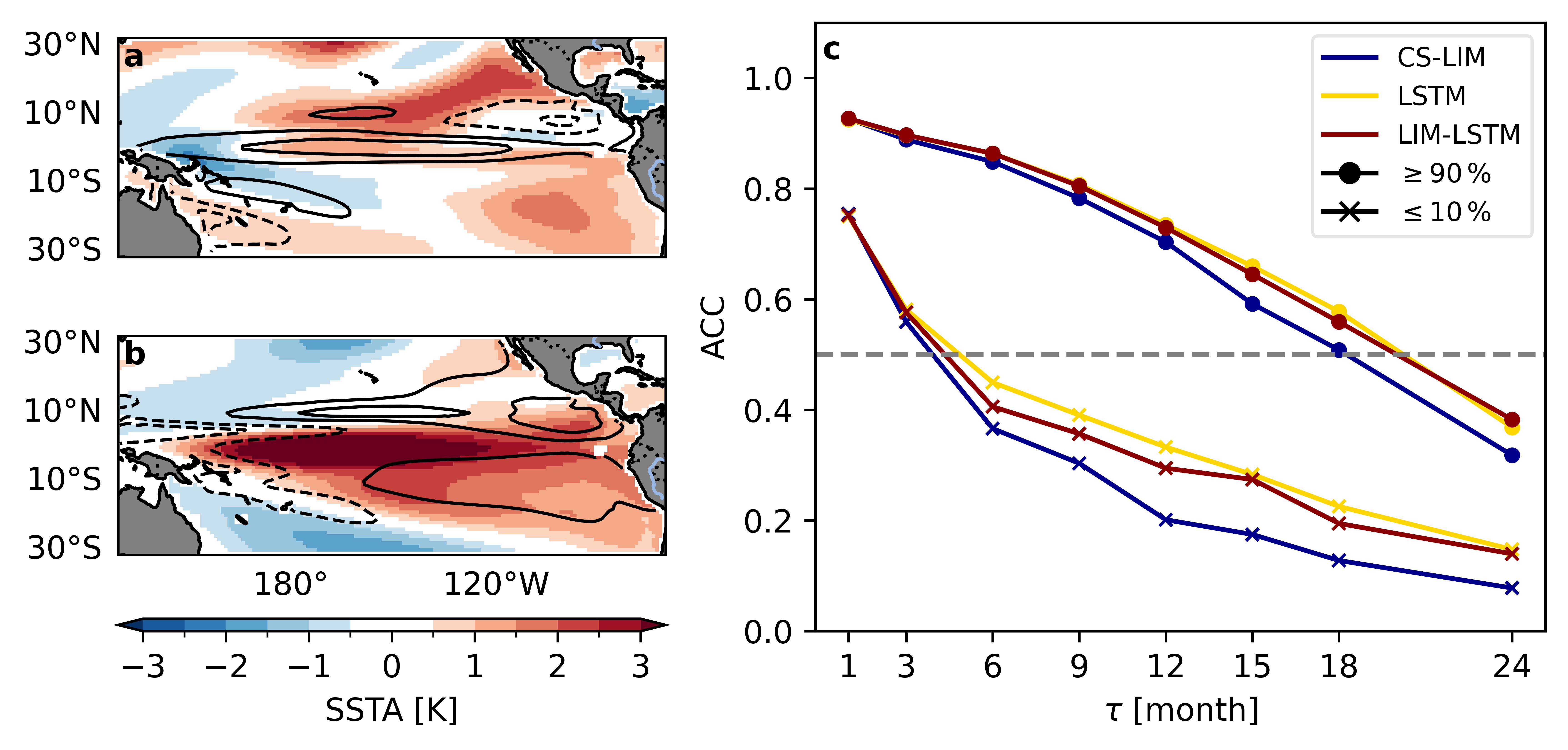
Previous LIM predictability studies have shown that the LIM can predict not only its own skill but, often, also that of operational prediction models (Newman and Sardeshmukh, 2017; Albers and Newman, 2019, 2021). We might exploit this ability by building our hybrid LIM-LSTM model on top of the LIM. For any given initial forecast state, the CS-LIM’s maximum predictability can be calculated by projecting the state onto the optimal initial condition (OIC) for a forecast lead time . The OIC is the singular vector corresponding to the largest singular value of the forecast propagator (see Methods 4.4). This condition is optimal in the sense that of all possible initial conditions of unit amplitude, it evolves into the largest amplitude (under the L2 norm) state vector at lead time (Penland and Sardeshmukh, 1995). For CS-LIM, we obtain a different OIC at every month and lead time.
The CS-LIM’s OIC for a 12-month forecast in April (Fig. 6a) exhibits an SST and SSH structure that aligns closely with earlier research (Newman et al., 2011; Vimont et al., 2014; Capotondi and Sardeshmukh, 2015). Key features of the OIC are: a band of positive SST anomalies in the northern subtropics, stretching diagonally from approximately 0°N, 180°W northeastward to around 30°N, 120°W; positive SST anomalies in the southern subtropics, predominantly east of 120°W; enhanced thermocline depth anomalies along the equator; and comparatively weak negative thermocline depth anomalies located at approximately 10°N in the eastern tropical Pacific. We obtain its subsequent evolution after months by applying the LIM operator to the OIC (Fig 6b). It is important to note that the magnitude of these patterns is arbitrary, a result of the unit norm of the singular vector.
The strength of the projection of the initial forecast state onto the CS-LIM -lead OIC, or how well the initial state matches the first singular vector – termed as optimal initial growth – is a key determinant of the potential forecast skill of the CS-LIM (Newman et al., 2003). To illustrate this point, for each forecast lead time ranging from 1-24 months, we select initial states from the test set whose projections on the OIC determined for that lead have either the least (0-10%) or greatest (90-100%) amplitudes, and then compute the forecast skill that results from forecasts made for each group separately. The average ACC, illustrated in Fig. 6c, is substantially larger for forecasts initialized from states with the strongest optimal initial growth than for states with minimal optimal initial growth, a result we could have anticipated at the time of forecast.
The dependence of skill upon the presence of (linear) optimal initial growth occurs not only for the CS-LIM but also for the LIM-LSTM hybrid model, although it also has a substantial skill increase compared to the CS-LIM (Fig. 6c). This result implies that optimal initial growth, although a property derived from the CS-LIM, influences not only linear predictability but also significantly impacts overall predictability of the entire system. This is further supported by the LSTM forecast, where a similar marked increase in skill is observed for initial states with the strongest optimal initial growth (i.e., cases where strong linear predictability is expected) as opposed to those with minimal initial growth.
2.4 ENSO asymmetry is nonlinearly predictable
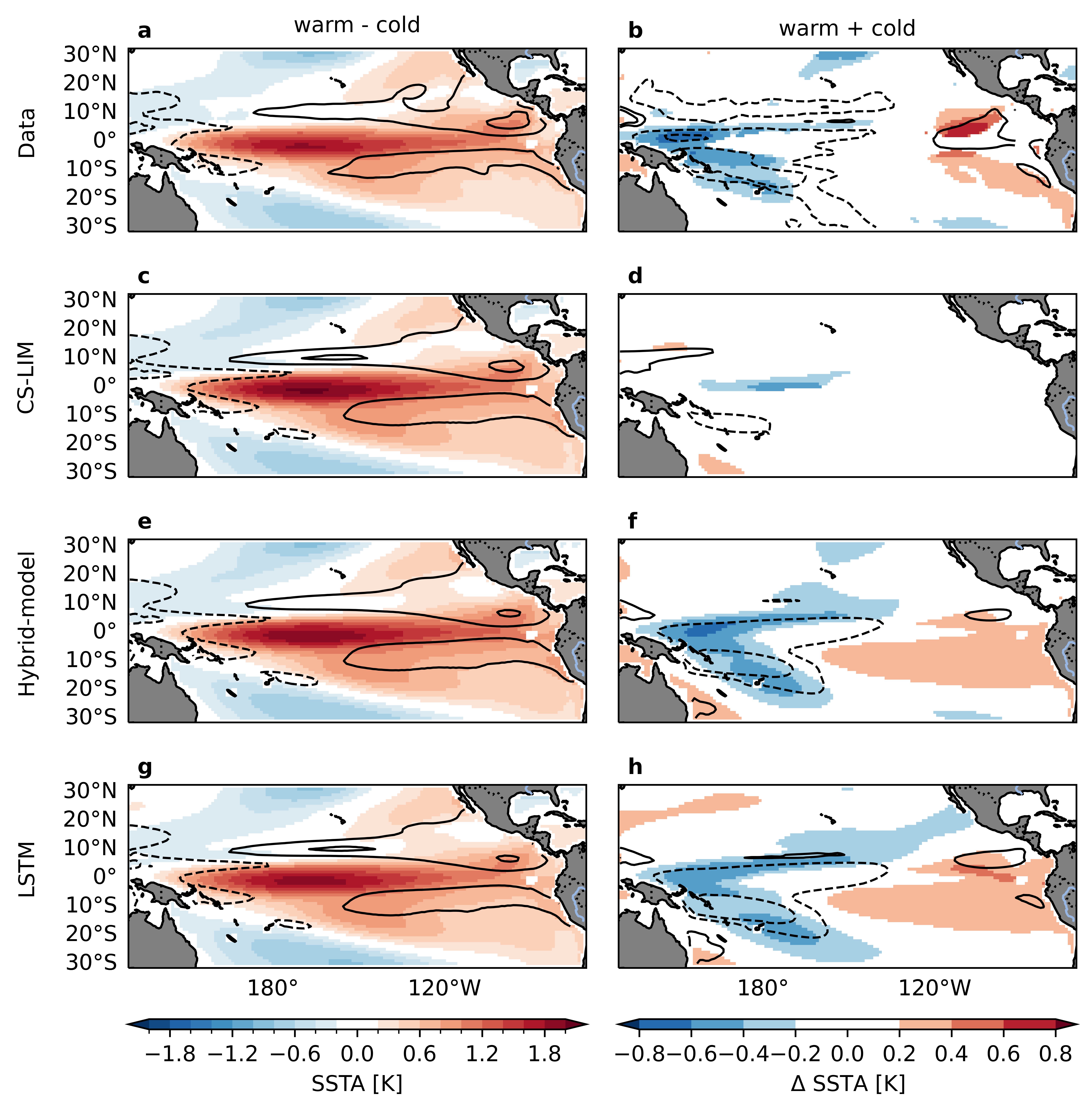
The initial states projected onto the OIC, shown in 6a, can yield either positive or negative optimal initial growth which evolve into warm or cold patterns, respectively. We examine the average month forecast of April initial states with the absolute largest optimal initial growth (>90%) for our CS-LIM, LIM-LSTM, and LSTM models.
The average forecast pattern’s magnitude and asymmetry are estimated by warm minus cold patterns (W-C, Fig. 7, first column) and warm plus cold patterns (W+C, Fig. 7, second column), respectively. A two-sided t-test is utilized to ascertain statistically significant difference between the means of the two distributions. We report only those values that surpass the 95% confidence interval threshold.
The W-C pattern in the target data (Fig. 7a) closely resembles the evolved optimal pattern of the CS-LIM (Fig. 6b) and its average empirical forecast (Fig. 7c). An evident east-west dipole structure is observed in the asymmetry of warm versus cold events of the target data (Fig. 7b). Cold events exhibit higher SSTA and SSHA magnitudes in the western tropical Pacific, while warm events show greater magnitudes in the Central-Eastern Pacific. This asymmetry is not present in the W+C patterns of the CS-LIM forecast (Fig. 7d) because of its linear and therefore symmetric evolution of cold and warm events. The remaining subtle differences between warm and cold patterns of CS-LIM forecast likely originate from the asymmetrical distribution of initial conditions, which might arise by chance but might also arise from a CAM noise process (not included in our CS-LIM), as noted earlier.
In contrast, the LIM-LSTM model and LSTM forecasts accurately capture both the magnitude and asymmetry of warm and cold events. Both nonlinear model forecasts exhibit the zonal dipole structure present in the target data (Fig. 7f and h). This finding highlights the ability of our nonlinear models to predict the asymmetry between warm and cold patterns. Note also that the predicted W-C component for both the LIM-LSTM and LSTM models is very similar to that of the CS-LIM (see Fig. 7c,e,g). This suggests that the hybrid model improves upon the CS-LIM by capturing predictable nonlinearity, rather than by finding additional linear skill. Taken together, these findings underscore the LIM-LSTM model’s potential to disentangle linear and nonlinear predictable dynamics, setting the stage for future systematic analysis of nonlinearities in subsequent work.
3 Discussion
We have introduced a LIM-LSTM hybrid model specifically tailored for forecasting SST and SSH anomalies in the tropical Pacific. We start from the LIM, an empirical model describing the dynamics of the slower-varying ocean as stochastically forced by the rapidly varying atmosphere, with its deterministic dynamics assumed to be linear. However, while the LIM produces ENSO forecasts comparable to state-of-the-art numerical models, it is unable to capture observed asymmetries of ENSO that are likely important to its predictability, especially for longer forecast leads.
We combine an LSTM with the LIM to capture predictable nonlinearities and non-Markovian dynamics in the evolution of monthly tropical SSTA. The LIM-LSTM model is trained and tested on SSTA and SSHA data from the CESM2 pre-industrial control run. We find that modeling nonlinearities significantly enhances the forecast accuracy, particularly in the western tropical Pacific within the 9 to 18-month range.
Our findings provide initial evidence that the asymmetry between warm and cold events is a key source of nonlinearity that improves forecasting skill beyond linear models. This first insight lays the groundwork for a more comprehensive follow-up characterization of the potential sources of nonlinearity of ENSO forecasting.
We demonstrate that the predictability of the LIM-LSTM model is strongly related to the theoretical expected skill of the LIM which allows us to reliably assess its predictability. In contrast, neural networks typically struggle to provide accurate predictability assessments on seasonal to annual scales, primarily hindered by their weak spread-to-skill relationship. Given that LIM models show competitive performance with GCMs (Newman and Sardeshmukh, 2017; Albers and Newman, 2019, 2021) and that the LIM-LSTM requires less data than a full LSTM, this hybrid LIM-LSTM is a promising approach for other S2S climate forecasts beyond ENSO.
A notable feature of our LIM-LSTM model is its data efficiency, particularly when compared to more data-intensive deep learning models like the LSTM network. This aspect is crucial given the limited span of available oceanic observational data. For a fair comparison, we utilized data from GCMs in our training, acknowledging their inherent biases as discussed in our study. The use of domain adaptation methods from deep learning emerges as a promising strategy to close the gap between GCM data and observational data. However, the field still needs more research to fully understand how neural network models can be adjusted to observational data when pre-trained on simulated data.
Although our models are based on LSTMs, which are not the most advanced deep learning models, they exhibit similar forecasting skill to the larger vision transformer model by Zhou and Zhang (Zhou and Zhang, 2023). This suggests that for the amount of observational data typically available to train data-driven models on seasonal time scales, hybrid models could outperform fully deep-learning models.
4 Materials and Methods
4.1 Data
Training DL models for ENSO prediction with monthly data is limited by the short observational record. To test the impact of record length on the data-driven models, we use the 2000-year CESM2 pre-industrial control simulation (Danabasoglu et al., 2020). We focus on monthly SST and SSH data in the tropical Pacific region (130°E - 70°W, 31°S - 32°N), which we linearly interpolate to a resolution of 1°x1°. SSH is a proxy for the upper ocean temperatures and the thermocline depth. Despite the lack of external forcing in the control simulation, we observe a trend in SST data. We linearly detrend the data and remove the seasonal cycle by subtracting the monthly climatology which is obtained over the training set (0-1500). As SSTA and SSHA differ in units and scales, we perform a -score normalization before model training. Both the LIM and LIM-LSTM model require us to reduce the dimensionality, which is achieved using Empirical Orthogonal Function (EOF) analysis. The dataset is divided into training (75%, year 1-1500), validation (15%, years 1500-1800), and test set (10%, 1800-2000), where the validation set is used for refining the hyperparameters of our models.
4.2 Methods
The objective of our study is to accurately predict SSTA and SSHA fields for a specified forecast lead time . We define the stacked variable fields at a given time as , where each field spans the tropical Pacific . We estimate a function , depending on month , that predicts the future state, at an incremental time step , by
| (1) |
The autoregressive prediction is based on the previous states, , referred to as history. All our model forecasts consist of ensemble members, which allows us to estimate the model uncertainty. The dynamics of the tropical Pacific Ocean show a strong seasonal phase locking. We therefore condition on the month of the year, . The month conditioning depends on the model architecture and will be discussed for each model separately.
4.3 Empirical Orthogonal Function (EOF)
Estimating the linear evolution operator of the LIM requires a matrix inversion of the number of input dimensions. The matrix inversion is intractable for the full spatial fields of SSTA and SSHA. For this reason, each state is transformed into a lower-dimensional state . Dimensionality reduction of the SSTA and SSHA fields in the tropical Pacific is achieved through EOF analysis, utilizing the first 20 Principal Components (PCs) for SSTA and the first 10 PCs for SSHA. Including higher-order PCs does not affect our results. Forecasting in the lower dimensional space is then equivalently conducted on these PCs, as formulated in Eq. 1. For analysis and evaluation, we transform our forecast back to grid space. To adequately replicate the high spatial frequencies of the input fields, we add variability by randomly sampling loadings of the higher-order PCs (20-300) for both SSTA and SSHA at each time step. These random features are then combined with their respective EOFs and added to the forecast fields, ensuring a closer match to the spatial intricacies of the original data.
4.4 Linear Inverse Model
The LIM describes the dynamic of the tropical Pacific as a multivariate linear system subject to stochastic forcing from the atmosphere. The underlying dynamics of such a system is described by a linear stochastic differential equation,
| (2) |
where is the linear operator describing the dynamics of and is a noise vector that is uncorrelated over time but spatially correlated, as encoded in the covariance matrix . Forecasts of for a lead time are given by the transition probability as,
| (3) |
| (4) |
where is the infinite ensemble mean forecast and is the forecast covariance matrix.
Penland and Sardeshmukh (1995) show that the linear operator and the noise covariance can be estimated from the data under two assumptions. First, the system has to be statistically stationary which allows us to write the Fluctuation-Dissipation relationship as
| (5) |
where is the spatial covariance matrix. Secondly, the autocorrelation of the system decays with lead time which can be expressed using the time-lead covariance matrix as
| (6) |
where is the Greens function that must tend to zero for long lead times. Typically, both assumptions hold for detrended anomaly data of a chaotic system.
Once and are estimated from the data, we obtain forecast trajectories from an initial time to , by numerically integrating eq. 2 using the forward Euler-method with incremental update steps as
| (7) |
where is a random sample from the noise distribution. We create ensemble member trajectories from to when integrating the system -times. The infinite ensemble member mean is given by in eq. 3.
In the equatorial Pacific, the variance in SSTA shows a distinct annual pattern with low variance during the boreal spring and high variance in the boreal winter. This peak in winter variance aligns with the occurrence of the most intense warm and cold ENSO events, a phenomenon referred to as "ENSO phase locking" (Rasmusson and Carpenter, 1982). Shin et al. (2021) showed that including seasonality in the LIM improves its forecast reliability. Their cyclostationary (CS)-LIM involves estimating unique linear operators and noise covariances for each month, indexed using . The numerical integration of the stationary (ST)-LIM outlined in eq. 7 changes to
| (8) |
where . The CS-LIM forms the base model of our LIM-LSTM model outlined in the following.
4.5 LIM-LSTM model
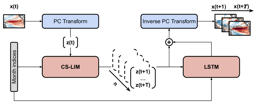
We introduce a novel LIM-LSTM model that combines the LIM with an LSTM network. While the LIM captures the predictable linear dynamics, the LSTM learns the residuals between the LIM predictions and the actual data, thus the nonlinear dynamics. Our methodology is schematically detailed in Fig. 8.
During inference, we project the initial state of the tropical Pacific, , onto the leading EOFs and employ the LIM to predict future states over timesteps. For each timestep, , we predict a correction, , to the LIM forecast, . The final forecast is thus defined as:
| (9) |
The nonlinear correction is modeled by the LSTM as , where is the latent state of the LSTM which aggregates the information of previous states. The LSTM is selected not only for its ability to capture nonlinear relationships inherent in deep neural networks but also for learning non-Markovian dynamics.
To include seasonality within the LSTM, we introduce a learned affine transformation to its latent state (Perez et al., 2017), , as follows:
| (10) |
where and represent embeddings for each month, enabling the network to adapt its latent state dynamically to seasonal variations.
The LSTM component is configured to process the forecast from each CS-LIM ensemble member, represented as . At each timestep, the input to the LSTM network is linearly projected into a higher-dimensional latent space where it is processed by two consecutive LSTM layers. By combining the LIM forecast at each timestep with the LSTM’s hidden state from the previous time step, the model iteratively accumulates information across the entire forecast sequence. Finally, the predicted latent states are linearly projected back onto the PCs and added to the original LIM prediction. The combined prediction is then transformed to grid space by multiplication with the respective EOFs, as described in sec. 4.24.3.
4.6 Purely deep learning baselines
To verify the utility of our LIM-LSTM model, we provide a comparison against fully neural network-based approaches. Similar to the structure of our LIM-LSTM model, we construct an LSTM that operates in the PC space. Additionally, we explore the application of a Convolutional LSTM (ConvLSTM (Shi et al., 2015)) architecture in grid space. We employ a custom ConvLSTM variant specifically tailored to perform forecasts on fields with large-scale spatial structures.
Both the PC-LSTM and the ConvLSTM have a standard Encoder-Decoder structure used for sequence-to-sequence modeling (Sutskever et al., 2014), as depicted in Fig. S1. Unlike the LIM and LIM-LSTM model, these models incorporate information from time points preceding the initialization time. The Encoder network is designed to aggregate this historical information into a latent state which initializes the Decoder model. It begins with a downsampling block that transforms the history into a higher-dimensional latent space, which is then processed by two LSTM layers, where the input is added to the hidden state from the previous time step. The hidden state of the second LSTM layer at time is then passed to the Decoder network. The Decoder mirrors the Encoder with two LSTM layers of its own, which do not require any additional input other than the hidden state and can thus be rolled out over the full prediction horizon , transferring the hidden state autoregressively for each successive prediction time. This is followed by an upsampling block that transforms the hidden state back to the input grid space. To generate 16-ensemble members, we employ a separate upsampling block for each member which are trained jointly. Similar to the LIM-LSTM model, we incorporate seasonal information through a learned affine transformation in both the Encoder and Decoder networks.
PC-LSTM
In the PC-LSTM, the downsampling consists of an EOF-truncation of the entire SSTA and SSHA fields onto their respective PCs (sec. 4.24.3), followed by a learned linear layer that projects the data into the latent space. The latent states are recursively predicted using LSTM layers, in both the encoder and the decoder network. Equivalently to the downsampling, the upsampling block starts with a linear layer to project the latent space back to the PCs, followed by a projectionon their respective EOFs to yield a forecast of the variables in grid space.
ConvLSTM
We employ a second DL model that does not involve EOF-truncation of data. This model is based-on the ConvLSTM (Shi et al., 2015) with a customized LSTM cell (Fig. S2). Unlike the PC-LSTM, the input, latent, and hidden states in our model maintain dimensions of channel, height, and width, albeit of varying sizes. For model input, both variables are stacked along the channel dimension. The encoder initially downscales the height and width dimensions to reduce computational costs, while simultaneously expanding the channel dimension via a strided convolutional layer. Following the methodology of Liu et al. (2021, 2022) we use equal stride and kernel sizes for this initial encoding, effectively partitioning the input into small patches of equal size (4x4 grid-steps in latitude/longitude direction). This method of dimensionality reduction differs from the EOF as it is learned end-to-end with the forecasting model, as well as being based on local patches, rather than global features as encoded in EOFs. Our approach further adapts the standard ConvLSTM layer, in a similar fashion to Liu et al. (2022), by splitting the convolution into spatial and channel mixing components, interspersed with layer normalizations, as depicted in Fig.S2. This modification facilitates two major improvements over standard ConvLSTMSs, (i) the spatial mixing component enables a substantially larger receptive field while reducing the number of parameters and (ii) the added normalization stabilizes training and supports conditioning on monthly embeddings, implemented through the affine transformation outlined in Eq.10. Finally, the mirrored Decoder network, which also consists of two ConvLSTM layers and a strided and transposed convolution, transforms the aggregated hidden state back into the full-resolution grid space. An ensemble of 16 separate final projection layers are used to generate a probabilistic prediction and the model is trained using the Ensemble CRPS as detailed below.
4.7 Optimization procedure
Each model is designed to produce a probabilistic prediction by generating an ensemble of 16 sequences. We train the models to enhance both the accuracy of individual predictions and the spread among ensemble members. This is achieved by employing the Continuous Ranked Probability Score (CRPS) for optimization. The CRPS is a probabilistic metric that compares the cumulative probability distribution (CDF) of the forecast to the CDF of the target. The target, , is a single observation, and thus its CDF is a step function. A perfect CRPS score of zero would be a Dirac delta-like predictive probability density function centered at the target, for which the CDF would be the same step-function as is for the target. The CRPS has an analytic expression for parametric distributions, like the Gaussian distribution, but also a statistical form for empirical distributions (Hersbach, 2000; Gneiting and Raftery, 2007).
For our -ensemble member prediction, we compute the pixel-wise CRPS for empirical distributions as,
| (11) |
where and are the -ensemble member prediction and the target value at each location . We optimize the parameters of each model by minimizing the averaged CRPS between the observed data, , and its ensemble forecast, , across all locations and lead . Using Eq. 11, we define our tailored loss function as:
| (12) |
To address the greater loss values at longer forecast leads, we introduce a power-law decaying weight over lead time, , where is an empirically set hyper-parameter.
4.8 Evaluation metrics
Our analysis of the models, all of which generate ensemble member predictions, is based on probabilistic metrics as well as deterministic metrics of their ensemble mean. We evaluate all models on the test set (200 years) using SSTA and SSHA in the tropical Pacific.
Anomaly correlation coefficient (ACC)
The ACC is the temporal correlation between the model forecast and the target at each spatial location over the test set. The ACC is defined as,
| (14) |
where is the covariance between the time series and their respective variance.
Root mean square error skill score (RMSESS)
The RMSESS is a deterministic metric that compares the RMSE of the model to the RMSE of a reference forecast. Throughout this work, we choose the climatology as our reference forecast. The RMSESS can be written as
| (15) |
where is the variance of the data. An RMSESS of 1 is a perfect model forecast and 0 is as good as the climatology forecast.
Continuous ranked probability skill score (CRPSS)
Equivalently to the skill score of the RMSE, we define the CRPS skill score using Eq. 11 as, , where the reference forecast is the climatology. A CRPSS of 1 is a perfect model forecast and 0 is as good as the climatology forecast.
Acknowledgements
The authors acknowledge funding by the Deutsche Forschungsgemeinschaft (DFG, German Research Foundation) under Germany’s Excellence Strategy – EXC number 2064/1 – Project number 390727645. Furthermore, we express our gratitude to the NOAA Physical Science Laboratory for making their resources available for this study. Antonietta Capotondi was supported by the NOAA Climate Program Office MAPP and CVP programs, and by DOE Award DE-SC0023228. We further thank the International Max Planck Research School for Intelligent Systems for supporting Jakob Schlör.
Data Availability Statement
All data used in this study are publicly available and are referenced in the main text or the supplementary materials. Our code is available at https://github.com/jakob-schloer/hybridLIM.
References
- Albers and Newman (2019) J. R. Albers and M. Newman. A Priori Identification of Skillful Extratropical Subseasonal Forecasts. Geophysical Research Letters, 46(21):12527–12536, 2019. ISSN 1944-8007. 10.1029/2019GL085270.
- Albers and Newman (2021) J. R. Albers and M. Newman. Subseasonal predictability of the North Atlantic Oscillation. Environ. Res. Lett., 16(4):044024, Mar. 2021. ISSN 1748-9326. 10.1088/1748-9326/abe781.
- Bauer et al. (2015) P. Bauer, A. Thorpe, and G. Brunet. The quiet revolution of numerical weather prediction. Nature, 525(7567):47–55, Sept. 2015. ISSN 1476-4687. 10.1038/nature14956.
- Ben-Bouallegue et al. (2023) Z. Ben-Bouallegue, M. C. A. Clare, L. Magnusson, E. Gascon, M. Maier-Gerber, M. Janousek, M. Rodwell, F. Pinault, J. S. Dramsch, S. T. K. Lang, B. Raoult, F. Rabier, M. Chevallier, I. Sandu, P. Dueben, M. Chantry, and F. Pappenberger. The rise of data-driven weather forecasting, July 2023.
- Beverley et al. (2023) J. D. Beverley, M. Newman, and A. Hoell. Rapid Development of Systematic ENSO-Related Seasonal Forecast Errors. Geophysical Research Letters, 50(10):e2022GL102249, 2023. ISSN 1944-8007. 10.1029/2022GL102249.
- Bi et al. (2023) K. Bi, L. Xie, H. Zhang, X. Chen, X. Gu, and Q. Tian. Accurate medium-range global weather forecasting with 3D neural networks. Nature, 619(7970):533–538, July 2023. ISSN 1476-4687. 10.1038/s41586-023-06185-3.
- Cachay et al. (2021) S. R. Cachay, E. Erickson, A. F. C. Bucker, E. Pokropek, W. Potosnak, S. Bire, S. Osei, and B. Lütjens. The World as a Graph: Improving El Ni\~no Forecasts with Graph Neural Networks, May 2021. URL http://arxiv.org/abs/2104.05089.
- Callahan and Mankin (2023) C. Callahan and J. S. Mankin. Persistent effect of El Niño on global economic growth | Science, 2023. URL https://www.science.org/doi/10.1126/science.adf2983.
- Capotondi (2013) A. Capotondi. ENSO diversity in the NCAR CCSM4 climate model: Enso Diversity in the NCAR CCSM4. J. Geophys. Res. Oceans, 118(10):4755–4770, Oct. 2013. ISSN 21699275. 10.1002/jgrc.20335.
- Capotondi and Sardeshmukh (2015) A. Capotondi and P. D. Sardeshmukh. Optimal precursors of different types of ENSO events. Geophysical Research Letters, 42(22):9952–9960, 2015. ISSN 1944-8007. 10.1002/2015GL066171.
- Capotondi et al. (2015) A. Capotondi, A. T. Wittenberg, M. Newman, E. D. Lorenzo, J. Y. Yu, P. Braconnot, J. Cole, B. Dewitte, B. Giese, E. Guilyardi, F. F. Jin, K. Karnauskas, B. Kirtman, T. Lee, N. Schneider, Y. Xue, and S. W. Yeh. Understanding enso diversity. Bulletin of the American Meteorological Society, 96(6):921–938, June 2015. ISSN 15200477. 10.1175/BAMS-D-13-00117.1.
- Capotondi et al. (2020) A. Capotondi, C. Deser, A. S. Phillips, Y. Okumura, and S. M. Larson. ENSO and Pacific Decadal Variability in the Community Earth System Model Version 2. Journal of Advances in Modeling Earth Systems, 12(12):e2019MS002022, 2020. ISSN 1942-2466. 10.1029/2019MS002022.
- Chen et al. (2016) C. Chen, M. A. Cane, N. Henderson, D. E. Lee, D. Chapman, D. Kondrashov, and M. D. Chekroun. Diversity, Nonlinearity, Seasonality, and Memory Effect in ENSO Simulation and Prediction Using Empirical Model Reduction. Journal of Climate, 29(5):1809–1830, Mar. 2016. ISSN 0894-8755, 1520-0442. 10.1175/JCLI-D-15-0372.1.
- Chen et al. (2021) H.-C. Chen, Fei-Fei-Jin, S. Zhao, A. T. Wittenberg, and S. Xie. ENSO Dynamics in the E3SM-1-0, CESM2, and GFDL-CM4 Climate Models. Journal of Climate, 34(23):9365–9384, Dec. 2021. ISSN 0894-8755, 1520-0442. 10.1175/JCLI-D-21-0355.1.
- Danabasoglu et al. (2020) G. Danabasoglu, J.-F. Lamarque, J. Bacmeister, D. A. Bailey, A. K. DuVivier, J. Edwards, L. K. Emmons, J. Fasullo, R. Garcia, A. Gettelman, C. Hannay, M. M. Holland, W. G. Large, P. H. Lauritzen, D. M. Lawrence, J. T. M. Lenaerts, K. Lindsay, W. H. Lipscomb, M. J. Mills, R. Neale, K. W. Oleson, B. Otto-Bliesner, A. S. Phillips, W. Sacks, S. Tilmes, L. van Kampenhout, M. Vertenstein, A. Bertini, J. Dennis, C. Deser, C. Fischer, B. Fox-Kemper, J. E. Kay, D. Kinnison, P. J. Kushner, V. E. Larson, M. C. Long, S. Mickelson, J. K. Moore, E. Nienhouse, L. Polvani, P. J. Rasch, and W. G. Strand. The Community Earth System Model Version 2 (CESM2). Journal of Advances in Modeling Earth Systems, 12(2):e2019MS001916, 2020. ISSN 1942-2466. 10.1029/2019MS001916.
- Dommenget et al. (2013) D. Dommenget, T. Bayr, and C. Frauen. Analysis of the non-linearity in the pattern and time evolution of El Niño southern oscillation. Clim Dyn, 40(11):2825–2847, June 2013. ISSN 1432-0894. 10.1007/s00382-012-1475-0.
- Frankignoul and Hasselmann (1977) C. Frankignoul and K. Hasselmann. Stochastic climate models, Part II Application to sea-surface temperature anomalies and thermocline variability. Tellus, 29(4):289–305, 1977. ISSN 2153-3490. 10.1111/j.2153-3490.1977.tb00740.x.
- Geng and Jin (2022) L. Geng and F.-F. Jin. ENSO Diversity Simulated in a Revised Cane-Zebiak Model. Frontiers in Earth Science, 10, 2022. ISSN 2296-6463. URL https://www.frontiersin.org/articles/10.3389/feart.2022.899323.
- Gneiting and Raftery (2007) T. Gneiting and A. E. Raftery. Strictly Proper Scoring Rules, Prediction, and Estimation. Journal of the American Statistical Association, 102(477):359–378, Mar. 2007. ISSN 0162-1459. 10.1198/016214506000001437.
- Gneiting et al. (2005) T. Gneiting, A. E. Raftery, A. H. Westveld, and T. Goldman. Calibrated Probabilistic Forecasting Using Ensemble Model Output Statistics and Minimum CRPS Estimation. Monthly Weather Review, 133(5):1098–1118, May 2005. ISSN 1520-0493, 0027-0644. 10.1175/MWR2904.1.
- Goel et al. (2017) H. Goel, I. Melnyk, and A. Banerjee. R2N2: Residual Recurrent Neural Networks for Multivariate Time Series Forecasting, Sept. 2017.
- Ham et al. (2019) Y.-G. Ham, J.-H. Kim, and J.-J. Luo. Deep learning for multi-year ENSO forecasts. Nature, 573(7775):568–572, Sept. 2019. ISSN 0028-0836, 1476-4687. 10.1038/s41586-019-1559-7.
- Hasselmann (1976) K. Hasselmann. Stochastic climate models Part I. Theory. Tellus, 28(6):473–485, 1976. ISSN 2153-3490. 10.1111/j.2153-3490.1976.tb00696.x.
- Hayashi et al. (2020) M. Hayashi, F.-F. Jin, and M. F. Stuecker. Dynamics for El Niño-La Niña asymmetry constrain equatorial-Pacific warming pattern. Nat Commun, 11(1):4230, Aug. 2020. ISSN 2041-1723. 10.1038/s41467-020-17983-y.
- Hersbach (2000) H. Hersbach. Decomposition of the Continuous Ranked Probability Score for Ensemble Prediction Systems. Weather and Forecasting, 15(5):559–570, Oct. 2000. ISSN 1520-0434, 0882-8156. 10.1175/1520-0434(2000)015<0559:DOTCRP>2.0.CO;2.
- Hochreiter and Schmidhuber (1997) S. Hochreiter and J. Schmidhuber. Long Short-Term Memory. Neural Computation, 9(8):1735–1780, Nov. 1997. ISSN 0899-7667. 10.1162/neco.1997.9.8.1735.
- Irrgang et al. (2021) C. Irrgang, N. Boers, M. Sonnewald, E. A. Barnes, C. Kadow, J. Staneva, and J. Saynisch-Wagner. Towards neural Earth system modelling by integrating artificial intelligence in Earth system science. Nat Mach Intell, 3(8):667–674, Aug. 2021. ISSN 2522-5839. 10.1038/s42256-021-00374-3.
- Johnson (2001) G. C. Johnson. The Pacific Ocean Subtropical cell surface limb. Geophysical Research Letters, 28(9):1771–1774, 2001. ISSN 1944-8007. 10.1029/2000GL012723.
- Kochkov et al. (2023) D. Kochkov, J. Yuval, I. Langmore, P. Norgaard, J. Smith, G. Mooers, J. Lottes, S. Rasp, P. Düben, M. Klöwer, S. Hatfield, P. Battaglia, A. Sanchez-Gonzalez, M. Willson, M. P. Brenner, and S. Hoyer. Neural General Circulation Models, Nov. 2023.
- Lam et al. (2023) R. Lam, A. Sanchez-Gonzalez, M. Willson, P. Wirnsberger, M. Fortunato, F. Alet, S. Ravuri, T. Ewalds, Z. Eaton-Rosen, W. Hu, A. Merose, S. Hoyer, G. Holland, O. Vinyals, J. Stott, A. Pritzel, S. Mohamed, and P. Battaglia. GraphCast: Learning skillful medium-range global weather forecasting, Aug. 2023.
- Lang et al. (2024) S. Lang, M. Alexe, M. Chantry, J. Dramsch, F. Pinault, B. Raoult, M. C. A. Clare, C. Lessig, M. Maier-Gerber, L. Magnusson, Z. B. Bouallègue, A. P. Nemesio, P. D. Dueben, A. Brown, F. Pappenberger, and F. Rabier. AIFS - ECMWF’s data-driven forecasting system, June 2024.
- Lessig et al. (2023) C. Lessig, I. Luise, B. Gong, M. Langguth, S. Stadler, and M. Schultz. AtmoRep: A stochastic model of atmosphere dynamics using large scale representation learning, Aug. 2023. URL http://arxiv.org/abs/2308.13280.
- L’Heureux et al. (2020) M. L. L’Heureux, A. F. Z. Levine, M. Newman, C. Ganter, J.-J. Luo, M. K. Tippett, and T. N. Stockdale. ENSO Prediction. In El Niño Southern Oscillation in a Changing Climate, chapter 10, pages 227–246. American Geophysical Union (AGU), 2020. ISBN 978-1-119-54816-4. 10.1002/9781119548164.ch10.
- Liu et al. (2021) Z. Liu, Y. Lin, Y. Cao, H. Hu, Y. Wei, Z. Zhang, S. Lin, and B. Guo. Swin Transformer: Hierarchical Vision Transformer using Shifted Windows, Aug. 2021.
- Liu et al. (2022) Z. Liu, H. Mao, C.-Y. Wu, C. Feichtenhofer, T. Darrell, and S. Xie. A ConvNet for the 2020s, Mar. 2022.
- Loshchilov and Hutter (2017) I. Loshchilov and F. Hutter. SGDR: Stochastic Gradient Descent with Warm Restarts, May 2017.
- Loshchilov and Hutter (2019) I. Loshchilov and F. Hutter. Decoupled Weight Decay Regularization, Jan. 2019.
- Martinez-Villalobos et al. (2018) C. Martinez-Villalobos, D. J. Vimont, C. Penland, M. Newman, and J. D. Neelin. Calculating State-Dependent Noise in a Linear Inverse Model Framework. Journal of the Atmospheric Sciences, 75(2):479–496, Feb. 2018. ISSN 0022-4928, 1520-0469. 10.1175/JAS-D-17-0235.1.
- Martinez-Villalobos et al. (2019) C. Martinez-Villalobos, M. Newman, D. J. Vimont, C. Penland, and J. David Neelin. Observed El Niño-La Niña Asymmetry in a Linear Model. Geophysical Research Letters, 46(16):9909–9919, 2019. ISSN 1944-8007. 10.1029/2019GL082922.
- Newman and Sardeshmukh (2017) M. Newman and P. D. Sardeshmukh. Are we near the predictability limit of tropical Indo-Pacific sea surface temperatures? Geophysical Research Letters, 44(16):8520–8529, Aug. 2017. ISSN 0094-8276, 1944-8007. 10.1002/2017GL074088.
- Newman et al. (2003) M. Newman, P. D. Sardeshmukh, C. R. Winkler, and J. S. Whitaker. A Study of Subseasonal Predictability. Monthly Weather Review, 131(8):1715–1732, Aug. 2003. ISSN 1520-0493, 0027-0644. 10.1175//2558.1.
- Newman et al. (2011) M. Newman, M. A. Alexander, and J. D. Scott. An empirical model of tropical ocean dynamics. Clim Dyn, 37(9-10):1823–1841, Nov. 2011. ISSN 0930-7575, 1432-0894. 10.1007/s00382-011-1034-0.
- Okumura (2019) Y. M. Okumura. ENSO Diversity from an Atmospheric Perspective. Curr Clim Change Rep, 5(3):245–257, Sept. 2019. ISSN 2198-6061. 10.1007/s40641-019-00138-7.
- Pathak et al. (2022) J. Pathak, S. Subramanian, P. Harrington, S. Raja, A. Chattopadhyay, M. Mardani, T. Kurth, D. Hall, Z. Li, K. Azizzadenesheli, P. Hassanzadeh, K. Kashinath, and A. Anandkumar. FourCastNet: A Global Data-driven High-resolution Weather Model using Adaptive Fourier Neural Operators, Feb. 2022.
- Penland (1996) C. Penland. A stochastic model of IndoPacific sea surface temperature anomalies. Physica D: Nonlinear Phenomena, 98(2):534–558, Nov. 1996. ISSN 0167-2789. 10.1016/0167-2789(96)00124-8.
- Penland and Sardeshmukh (1995) C. Penland and P. D. Sardeshmukh. The Optimal Growth of Tropical Sea Surface Temperature Anomalies. Journal of Climate, 8(8):1999–2024, Aug. 1995. ISSN 0894-8755, 1520-0442. 10.1175/1520-0442(1995)008<1999:TOGOTS>2.0.CO;2.
- Perez et al. (2017) E. Perez, F. Strub, H. de Vries, V. Dumoulin, and A. Courville. FiLM: Visual Reasoning with a General Conditioning Layer, Dec. 2017.
- Petersik and Dijkstra (2020) P. J. Petersik and H. A. Dijkstra. Probabilistic Forecasting of El Niño Using Neural Network Models. Geophys. Res. Lett., 47(6), Mar. 2020. ISSN 0094-8276, 1944-8007. 10.1029/2019GL086423.
- Rasmusson and Carpenter (1982) E. M. Rasmusson and T. H. Carpenter. Variations in Tropical Sea Surface Temperature and Surface Wind Fields Associated with the Southern Oscillation/El Niño. Monthly Weather Review, 110(5):354–384, May 1982. ISSN 1520-0493, 0027-0644. 10.1175/1520-0493(1982)110<0354:VITSST>2.0.CO;2.
- Rasp and Lerch (2018) S. Rasp and S. Lerch. Neural Networks for Postprocessing Ensemble Weather Forecasts. Monthly Weather Review, 146(11):3885–3900, Nov. 2018. ISSN 1520-0493, 0027-0644. 10.1175/MWR-D-18-0187.1.
- Rodrigues et al. (2021) E. Rodrigues, B. Zadrozny, C. Watson, and D. Gold. Decadal Forecasts with ResDMD: A Residual DMD Neural Network, June 2021. URL http://arxiv.org/abs/2106.11111.
- Sardeshmukh and Penland (2015) P. D. Sardeshmukh and C. Penland. Understanding the distinctively skewed and heavy tailed character of atmospheric and oceanic probability distributions. Chaos: An Interdisciplinary Journal of Nonlinear Science, 25(3):036410, Mar. 2015. ISSN 1054-1500. 10.1063/1.4914169.
- Sardeshmukh et al. (2015) P. D. Sardeshmukh, G. P. Compo, and C. Penland. Need for Caution in Interpreting Extreme Weather Statistics. Journal of Climate, 28(23):9166–9187, Dec. 2015. ISSN 0894-8755, 1520-0442. 10.1175/JCLI-D-15-0020.1.
- Shi et al. (2015) X. Shi, Z. Chen, H. Wang, D.-Y. Yeung, W.-k. Wong, and W.-c. Woo. Convolutional LSTM Network: A Machine Learning Approach for Precipitation Nowcasting, Sept. 2015.
- Shin et al. (2021) S.-I. Shin, P. D. Sardeshmukh, M. Newman, C. Penland, and M. A. Alexander. Impact of Annual Cycle on ENSO Variability and Predictability. Journal of Climate, 34(1):171–193, Jan. 2021. ISSN 0894-8755, 1520-0442. 10.1175/JCLI-D-20-0291.1.
- Strnad et al. (2022) F. M. Strnad, J. Schlör, C. Fröhlich, and B. Goswami. Teleconnection Patterns of Different El Niño Types Revealed by Climate Network Curvature. Geophysical Research Letters, 49(17):e2022GL098571, 2022. ISSN 1944-8007. 10.1029/2022GL098571.
- Sutskever et al. (2014) I. Sutskever, O. Vinyals, and Q. V. Le. Sequence to Sequence Learning with Neural Networks, Dec. 2014.
- Takahashi and Dewitte (2016) K. Takahashi and B. Dewitte. Strong and moderate nonlinear El Niño regimes. Climate Dynamics, 46(5-6):1627–1645, Mar. 2016. ISSN 14320894. 10.1007/s00382-015-2665-3.
- Takahashi et al. (2011) K. Takahashi, A. Montecinos, K. Goubanova, and B. Dewitte. ENSO regimes: Reinterpreting the canonical and Modoki El Niño. Geophysical Research Letters, 38(10):L10704, May 2011. ISSN 00948276. 10.1029/2011GL047364.
- Takahashi et al. (2019) K. Takahashi, C. Karamperidou, and B. Dewitte. A theoretical model of strong and moderate El Niño regimes. Clim Dyn, 52(12):7477–7493, June 2019. ISSN 1432-0894. 10.1007/s00382-018-4100-z.
- Taschetto et al. (2020) A. S. Taschetto, C. C. Ummenhofer, M. F. Stuecker, D. Dommenget, K. Ashok, R. R. Rodrigues, and S.-W. Yeh. ENSO Atmospheric Teleconnections. In El Niño Southern Oscillation in a Changing Climate, chapter 14, pages 309–335. American Geophysical Union (AGU), 2020. ISBN 978-1-119-54816-4. 10.1002/9781119548164.ch14.
- Thual and Dewitte (2023) S. Thual and B. Dewitte. ENSO complexity controlled by zonal shifts in the Walker circulation. Nat. Geosci., 16(4):328–332, Apr. 2023. ISSN 1752-0908. 10.1038/s41561-023-01154-x.
- Timmermann et al. (2018) A. Timmermann, S.-I. An, J.-S. Kug, F.-F. Jin, W. Cai, A. Capotondi, K. M. Cobb, M. Lengaigne, M. J. McPhaden, M. F. Stuecker, K. Stein, A. T. Wittenberg, K.-S. Yun, T. Bayr, H.-C. Chen, Y. Chikamoto, B. Dewitte, D. Dommenget, P. Grothe, E. Guilyardi, Y.-G. Ham, M. Hayashi, S. Ineson, D. Kang, S. Kim, W. Kim, J.-Y. Lee, T. Li, J.-J. Luo, S. McGregor, Y. Planton, S. Power, H. Rashid, H.-L. Ren, A. Santoso, K. Takahashi, A. Todd, G. Wang, G. Wang, R. Xie, W.-H. Yang, S.-W. Yeh, J. Yoon, E. Zeller, and X. Zhang. El Niño–Southern Oscillation complexity. Nature, 559(7715):535–545, July 2018. ISSN 0028-0836, 1476-4687. 10.1038/s41586-018-0252-6.
- Vimont et al. (2014) D. J. Vimont, M. A. Alexander, and M. Newman. Optimal growth of Central and East Pacific ENSO events. Geophys. Res. Lett., 41(11):4027–4034, June 2014. ISSN 00948276. 10.1002/2014GL059997.
- Vimont et al. (2022) D. J. Vimont, M. Newman, D. S. Battisti, and S.-I. Shin. The Role of Seasonality and the ENSO Mode in Central and East Pacific ENSO Growth and Evolution. Journal of Climate, 35(11):3195–3209, June 2022. ISSN 0894-8755, 1520-0442. 10.1175/JCLI-D-21-0599.1.
- Wang et al. (2021) S. Wang, L. Mu, and D. Liu. A hybrid approach for El Niño prediction based on Empirical Mode Decomposition and convolutional LSTM Encoder-Decoder. Computers & Geosciences, 149:104695, Apr. 2021. ISSN 0098-3004. 10.1016/j.cageo.2021.104695.
- Watt-Meyer et al. (2021) O. Watt-Meyer, N. D. Brenowitz, S. K. Clark, B. Henn, A. Kwa, J. McGibbon, W. A. Perkins, and C. S. Bretherton. Correcting Weather and Climate Models by Machine Learning Nudged Historical Simulations. Geophysical Research Letters, 48(15):e2021GL092555, 2021. ISSN 1944-8007. 10.1029/2021GL092555.
- Wittenberg (2009) A. T. Wittenberg. Are historical records sufficient to constrain ENSO simulations? Geophysical Research Letters, 36(12):L12702, 2009. ISSN 1944-8007. 10.1029/2009GL038710.
- Zhou and Zhang (2022) L. Zhou and R.-H. Zhang. A Hybrid Neural Network Model for ENSO Prediction in Combination with Principal Oscillation Pattern Analyses. Adv. Atmos. Sci., 39(6):889–902, June 2022. ISSN 1861-9533. 10.1007/s00376-021-1368-4.
- Zhou and Zhang (2023) L. Zhou and R.-H. Zhang. A self-attention–based neural network for three-dimensional multivariate modeling and its skillful ENSO predictions. Sci. Adv., 9(10):eadf2827, Mar. 2023. ISSN 2375-2548. 10.1126/sciadv.adf2827.
Appendix A Supplementary Materials
A.1 Seasonal skill dependency

In addition to assessing the spatial distribution of skill (sec. 2.1), we investigate the seasonal skill variation. The average RMSESS of the Niño4 SSTA from the CS-LIM forecast, evaluated over different lead times and verification months, indicates that late winter and spring months are better predicted than the late summer and fall (Fig. S3a). These results are consistent with the findings by Shin et al. (2021), and align with the phenomenon known as the spring predictability barrier, characterized by a notable drop in the autocorrelation of the tropical Pacific SSTA in boreal spring.
For the LIM-LSTM model forecast, we observe the most significant RMSESS improvements upon the CS-LIM at lead times ranging between 9 and 18 months (Fig. S3b). Specifically, the maximum enhancements are seen at 15 and 18 months during the winter months (December to February), while in spring, the peak skill improvement is at a lead time of 12 months.