Monogamy of entanglement inspired protocol to quantify bipartite entanglement using spin squeezing

Abstract

Quantum entanglement is an essential resource for several branches of quantum science and technology, however, entanglement detection can be a challenging task, specifically, if typical entanglement measures such as linear entanglement entropy or negativity are the metrics of interest. Here we propose a protocol to detect bipartite entanglement in a system of $N$ qubits inspired by the concept of monogamy of entanglement. We argue that given a total system with some bipartite entanglement between two subsystems, subsequent unitary evolution, and measurement of one of the individual subsystems might be used to quantify the entanglement between the two. To address the difficulty of detection, we propose to use spin squeezing to quantify the entanglement within the individual subsystem, knowing that the relation between spin squeezing and some entanglement measures is not one-to-one, we give some suggestions on how a clever choice of squeezing Hamiltonian can lead to better results in our protocol. For systems with a small number of qubits, we derive analytical results and show how our protocol can work optimally for GHZ states, moreover, for larger systems we show how the accuracy of the protocol can be improved by a proper choice of the squeezing Hamiltonian. Our protocol presents an alternative for entanglement detection in platforms where state tomography is inaccessible (in widely separated entangled systems, for example) or hard to perform, additionally, the ideas presented here can be extended beyond spin-only systems to expand its applicability.

I Introduction

Entanglement is a fundamental feature of quantum mechanics that has puzzled scientists since the early days of its formulation [1, 2, 3]. Apart from generating interesting philosophical discussions, quantum entanglement is an essential asset for applications in multiple quantum science fields such as quantum teleportation [4, 5, 6], quantum cryptography [7], quantum metrology [8], and quantum computation [9].

In general, we can think of the study of entanglement as divided into three questions: (i) How is entanglement generated? (ii) How is entanglement quantified? and (iii) How is entanglement detected? In this work, we focus mostly on the second and third points but it is important to mention that, in the last couple of decades, great progress has been achieved in the generation of entanglement in photons [10, 11, 12], trapped ions [13, 14, 15, 16], and large ensembles of atoms in cavity QED setups [17, 18, 19], among other platforms.

Regarding entanglement quantification, various entanglement measures and inequalities have been proposed in the past decades, for a complete review of them, see [20]. For pure states, inequalities based on quantities such as entanglement entropy and linear entropy can be used to quantify the degree of entanglement in a system [21]. In the case of mixed states, entanglement quantification is more complex due to the presence of classical correlations. A well-studied alternative is the use of quantum negativity, which is numerically accessible for both pure and mixed states [22, 23], nonetheless, other measures of entanglement, such as the entanglement of formation [24] and relative entanglement entropy [25], stemming from concepts of distillable entanglement and entanglement cost, respectively, can be used to quantify entanglement in mixed states.

Regarding experimental entanglement detection, characterizing entanglement using the above measures can be a difficult task. Even in the case of pure states, obtaining the entanglement entropy would require quantum state tomography which might not always be accessible or easy to perform [26, 27], especially as the system size increases. An entanglement witness [28] is defined as a measurable observable that can help distinguish between an entangled state and a separable one; in a spin-only system, spin-squeezing parameters can be used to detect entanglement [29]. Measurements of spin-squeezing might not always quantify entanglement accurately [30] [31], nonetheless, spin-squeezed states are interesting in their own right as they have extensive applications in quantum metrology [32, 33].

In this work, we explore the application of spin-squeezing parameters of a subsystem to quantify the entanglement entropy of the full system, indirectly. This is particularly useful in situations where full-state tomography is not possible, for instance when one controls only one of the subsystems rather than the entire one. As we show here, the relationship between spin squeezing in the subsystem and the entanglement of the full system is closely related to the concept of monogamy of entanglement, which has been well understood since the early 2000’s [34, 35]. The prototypical example of monogamy of entanglement involves three qubits A, B, and C. The monogamy property states that the entanglement between A and B will limit the entanglement between A and C, illustrating that the amount of information that A can share with other qubits is constrained. In particular, if A and B are maximally entangled, neither A nor B can share any entanglement with C. The statement can be extended to the case of $N$ qubits where A can only share a fixed amount of information with the other $N-1$ qubits [36]. In a recent paper [37], this property was generalized to the case where A, B, and C each describe a subsystem of an arbitrary tripartite quantum system in a pure state. The monogamy inequality is then interpreted geometrically in the form of a triangular relation. Other generalized versions of the monogamy criteria can be found in [38].

In this study, we are interested in a generalization of the monogamy of entanglement concept, schematically depicted in Fig.1. We consider a total system divided into two subsystems A and B, each one composed of $N_{A}$ and $N_{b}$ two-level systems, respectively.

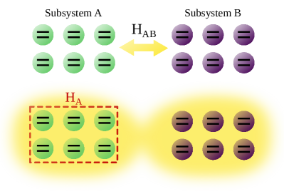
Figure 1: Schematics of the problem. Subsystem A contains $N_{A}$ two-level systems and subsystem B contains $N_{B}$. First, through $H_{AB}$ the two subsystems get entangled. Then, subsequent evolution using $H_{A}$ entangles the elements within subsystem A without changing the bipartite entanglement between A and B.

First, the entire system is subject to the action of Hamiltonian $H_{AB}$ which might create some bipartite entanglement between A and B. Subsequently, a Hamiltonian $H_{A}$ acts locally on subsystem A. The action of this Hamiltonian might create entanglement within the elements of A but its locality prevents any further modification of the bipartite entanglement between A and B. How is the entanglement generation within A affected by the pre-existing bipartite entanglement between A and B, and whether we can use the information obtained through the action of $H_{A}$ to learn about the bipartite entanglement between A and B are the main questions we will be addressing. Moreover, we explore if these relationships can be studied in terms of easily measurable observables such as spin-squeezing parameters.

This paper is organized as follows. First, we introduce different types of bipartite entanglement measures to be adopted in the paper. Second, we study the complexity of the generalized monogamy property by investigating two simple cases where analytical expressions for the entanglement measures can be derived. Next, we introduce our general protocol for quantifying the entanglement between A and B through local operations and measurements on A. We then discuss how spin-squeezing parameter measurements are related to bipartite entanglement for different typical Hamiltonians such as one-axis twisting (OAT) or two-axis twisting (TAT), and how to decide which of them might be more effective in different steps of our protocol. Finally, we test how our protocol performs in systems with different numbers of spins and reflect on its limitations and advantages.

II Bipartite Entanglement Measures

In this section, we introduce the bipartite entanglement measures we are going to use in this work. We shall start with entropy measures for a pure state. Consider a bipartite system described by the density matrix $\rho_{AB}$ and the corresponding reduced density matrices $\rho_{A}$ and $\rho_{B}$, the Tsallis entropy is defined as:

$$T_{\alpha}(\rho)=\frac{1-\text{Tr}(\rho^{q})}{q-1},$$ (1)

with $q$ being a positive integer and $\rho$ being a density matrix. It can be shown that the inequality $T_{q}(\rho_{AB})-T_{q}(\rho_{A})\geq 0$ holds for all separable states [39]. If the composite system $\rho_{AB}$ is in a pure state such that the first term in the inequality vanishes, the bipartite entanglement can then be characterized by $T_{q}(\rho_{A})=T_{q}(\rho_{B})$. For $q=1,2$, $T_{q}$ reduces to Von-Neumann entropy and linear entropy, respectively. To compare the entropy of systems with different sizes, we adopt a normalized form of linear entropy:

$$S_{L}(\rho)=\frac{N}{N-1}(1-\text{Tr}(\rho^{2})),$$ (2)

where $N$ is the dimension of the Hilbert space of $\rho$.

For more general states (pure or mixed), we first consider the entanglement negativity. The positive partial transpose (PPT) criterion, (or Peres-Horodecki criterion), is a necessary condition for separability which states that, for any separable state, the partial transpose of the composite density matrix, $\rho^{T_{A}}_{AB}$ (or equivalently $\rho^{T_{B}}_{AB}$), is positive [40, 22]. For systems of size $2\otimes 2$ and $2\otimes 3$, the PPT condition is also proved to be sufficient. Negativity is a computable entanglement measure introduced to quantify the violation of the PPT condition and it is defined by:

$$N_{0}(\rho)=\sum_{\lambda_{i}^{T_{A}}<0}|\lambda_{i}^{T_{A}}|,$$ (3)

where $\lambda^{T_{A}}_{i}$ are the eigenvalues $\rho^{T_{A}}_{AB}$. For separable states $N_{0}(\rho)=0$ while $N_{0}(\rho)>0$ indicates the presence of entanglement. The number of states with $N_{0}(\rho)>0$ can be used as an upper bound for the volume of entangled states for systems of sizes larger than $2\otimes 3$ [35]. Again for convenience of comparison, we introduce a normalized negativity $N(\rho)=N_{0}(\rho)/\max{(N_{0}(\rho))}$ such that the maximum available negativity for a system equals one.

The second measure we adopt for generic quantum states is concurrence. For an arbitrary two-qubit state, concurrence is equivalent to the entanglement of formation measure, which quantifies the amount of entanglement required to create such state [24, 41], and it is defined mathematically as:

$$C(\rho)=\text{max}(0,\mu_{1}-\mu_{2}-\mu_{3}-\mu_{4})$$ (4)

Where $\mu_{j}$ are the eigenvalues of the matrix $\tilde{\rho}=\rho S\rho^{*}S$, and $S=\sigma_{y}\otimes\sigma_{y}$, with $\sigma_{y}$ being the conventional Pauli matrix acting on each qubit subspace. Here, $\mu_{1}\geq\mu_{2}\geq\mu_{3}\geq\mu_{4}$. If $C(\rho)=0$ the state is separable and if $C(\rho)=1$ the state is maximally entangled.

III The Generalized Monogamy of Entanglement

In this section, we study the proposed generalized monogamy property in two specific spin systems.

We start by considering the simplest model for the setup in Fig. 1 with three qubits labeled by $A_{1}$, $A_{2}$, and B. Both $A_{1}$ and $A_{2}$ are regarded as elements of subsystem A, while subsystem $B$ is composed of a single qubit. We consider a system initialized in a pure state. We want to study the relation of the following quantities: (1) entanglement between the bipartite subsystems A and B, and (2) the maximum entanglement that can be created inside subsystem A, that is, between $A_{1}$ and $A_{2}$, through unitary evolution. We refer to this relation as the generalized monogamy of entanglement, which illustrates how the bipartite entanglement between A and B modifies the potential entanglement between the components of A.

Let the reduced density matrix for subsystem A be $\rho_{A}$ and that for B be $\rho_{B}$. According to the Schmidt decomposition $\rho_{A}$ and $\rho_{b}$ share the same spectrum:

$$\rho_{A}=\sum_{k=1}^{2}\lambda_{k}|\lambda_{k}\rangle\langle\lambda_{k}|,\quad\rho_{B}=\sum_{k=1}^{2}\lambda_{k}|\beta_{k}\rangle\langle\beta_{k}|.$$ (5)

For clarity, $\lambda_{k}$ will always refer to the eigenvalues of the reduced density matrices of the subsystems throughout this article. The decomposition on Eq. (5) shows that although subsystem A is a four-level system, we can understand its entanglement behavior by using a reduced two-level description. In that sense, system AB is effectively a two-qubit system, consequently, the entanglement between A and B can be quantified through concurrence. Direct evaluation of Eq. (4) gives:

$$C_{AB}=2\sqrt{\text{det}(\rho_{A})}=2\sqrt{\lambda_{1}-\lambda_{1}^{2}}.$$ (6)

In this specific case, the tangle $\tau_{AB}\equiv C_{AB}^{2}$ [34] is also equal to the linear entropy defined in Eq. (2).

To further investigate the maximum entanglement that can be created between $A_{1},A_{2}$, we use the result in Ref. [42] which states that for a generic two-qubit system represented by density matrix $\rho$ with eigenvalues ${\tilde{\lambda}_{1},\tilde{\lambda}_{2},\tilde{\lambda}_{3},\tilde{\lambda}_{4}}$ in descending order, the maximum allowed entanglement can be characterized by the maximum concurrence as:

$$C_{\text{max}}=\max(0,\tilde{\lambda}_{1}-\tilde{\lambda}_{3}-2\sqrt{\tilde{\lambda}_{2}\tilde{\lambda}_{4}}).$$ (7)

In our case, the density matrix we are interested in is $\rho_{A}$ and since $\lambda_{3}=\lambda_{4}=0$ according to Eq. (5), the above equation reduces to:

$$C_{A_{1}A_{2}}^{max}=\lambda_{1}\,,$$ (8)

where we have assumed $\lambda_{1}>\lambda_{2}$. Combining Eqs. (6) and (8):

$$\left(C_{AB}\right)^{2}=4C_{A_{1}A_{2}}^{max}-4(C_{A_{1}A_{2}}^{max})^{2}$$ (9)

Given that $\rho_{A}$ has a trace equal to one, it follows that $1\geq\lambda_{1}\geq 1/2$, consequently, the above relation is monotonic and one-to-one allowing to obtain an inverse relation:

$$C_{A_{1}A_{2}}^{max}=\frac{1}{2}\left[1+\sqrt{1-(C_{A,B})^{2}}\right]\,.$$ (10)

In Fig. 2, the relation between $C_{A_{1}A_{2}}$ and $C_{AB}$ is shown for a set of randomly sampled three-qubit pure states. The dashed line represents Eq.(10) and it is very clear from the figure that this expression is indeed the maximum value of $C_{A_{1}A_{2}}$ that can be obtained for a given $C_{AB}$. This monotonic relation is used as a motivation for our protocol proposal in the next section.

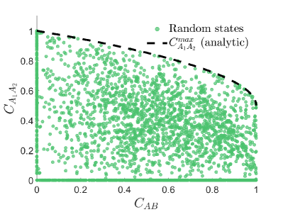
Figure 2: $C_{A_{1}A_{2}}$ as a function of $C_{AB}$ for a set of 3000 randomly sampled three-qubit pure states. The dashed line represent the analytic expression for the maximum $C_{A_{1}A_{2}}$ allowed (Eq. (10)).

To study larger systems, where we increase the number of qubits in B while keeping A being a two-qubit system, we shall also examine the relations above using negativity since the entanglement of formation becomes hard to compute. We first derive a similar relation as Eq. (10) for a pure three-qubit state in terms of negativity. Explicitly writing out the partial transpose of $\rho_{AB}$ and solving for the eigenvalues, we obtain the normalized negativity (see Appendix A):

$$N_{AB}=2\sqrt{\lambda_{1}(1-\lambda_{1})}$$ (11)

where the factor of two ensures normalization. In Ref. [42] authors presented that, for a general two-qubit system described by a density matrix $\rho$ with eigenvalues ${\tilde{\lambda}_{1},\tilde{\lambda}_{2},\tilde{\lambda}_{3},\tilde{\lambda}_{4}}$ in descending order, the maximum normalized negativity is given by:

$$N^{max}(\rho)=\text{max}(0,\sqrt{(\tilde{\lambda}_{1}-\tilde{\lambda}_{3})^{2}+(\tilde{\lambda}_{2}-\tilde{\lambda}_{4})^{2}}-\tilde{\lambda}_{2}-\tilde{\lambda}_{4}).$$ (12)

Again, with $\lambda_{3}=\lambda_{4}=0$, combining Eqs. (11) and (12) we find that the maximum negativity within subsystem A can be written as a function of the negativity between A and B:

$$N_{A_{1}A_{2}}^{max}=\frac{1}{2}\left(-1+\sqrt{4-2N_{AB}^{2}}+\sqrt{1-N_{AB}^{2}}\right)\,,$$ (13)

which, as expected, shows a monotonic one-to-one relation similar to Eq. (10).

Moving forward, if we keep subsystem A to be composed of only qubits $A_{1}$ and $A_{2}$ but now allow subsystem B to contain $N$ qubits with $N\geq 2$, the pure state of the system can be described by:

$$|\psi\rangle=\sum_{i=1}^{4}{\sqrt{\lambda_{i}}\left|\lambda_{i}\right\rangle\otimes\left|\beta_{i}\right\rangle}\,.$$ (14)

Now we have at most four non-zero eigenvalues of the respective reduced density matrices for A and B. The representation of the density matrix can be reduced to an effective $16\times 16$ matrix independent of $N$, with six possible negative eigenvalues: $-\sqrt{\lambda_{1}\lambda_{2}}$, $-\sqrt{\lambda_{1}\lambda_{3}}$, $-\sqrt{\lambda_{2}\lambda_{3}}$, $-\sqrt{\lambda_{1}\lambda_{4}}$, $-\sqrt{\lambda_{2}\lambda_{4}}$, $-\sqrt{\lambda_{3}\lambda_{4}}$, and the negativity would be given by the sum of the absolute values of each of them. The maximum negativity following Eq. (3) is $N_{0}=3/2$ when all $\lambda_{i}$ are identical. Hence we define the normalized negativity for $AB$ as:

$$N_{AB}=\frac{1}{3}\sum_{i,j=1}^{4}(1-\delta_{ij})\sqrt{\lambda_{i}\lambda_{j}}\,.$$ (15)

Note that we recover the case for $N=1$, up to a constant rescaling of $1/3$, when $\lambda_{3}=\lambda_{4}=0$, as expected. For this $2+N$ case $N^{max}_{AB}$ is given by Eq. (12) which cannot be further simplified, in general. In Fig. 3 we show the relation between the two relevant quantities for $2+1$ and $2+N$ systems.

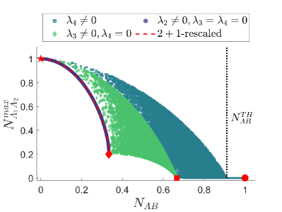
Figure 3: $N^{max}_{A_{1}A_{2}}$ as a function of $N_{AB}$. The markers represent $10^{5}$ randomly sampled points for a $2+N$ system. The sampling is done by randomly choosing the four eigenvalues $\lambda_{1}$, $\lambda_{2}$, $\lambda_{3}$, and $\lambda_{4}$ of the reduced density matrix. Purple circles (below red dashed line) represent the states for which $\lambda_{3}=\lambda_{4}=0$, green diamonds the states where $\lambda_{4}=0$, and blue squares the states where all eigenvalues are non-zero. Red markers signal representative boundary states defined explicitly in the main text. The red dashed line represents the monotonic expression for a $2+1$ system in Eq.(13) after being re-scaled by a factor of 1/3, while the vertical dotted line illustrates the threshold value of the negativity.

We sample different states $\rho_{AB}$ by randomly choosing the four eigenvalues $\lambda_{1}$, $\lambda_{2}$, $\lambda_{3}$, and $\lambda_{4}$ for the reduced density matrix $\rho_{A}$, we compute the negativity $N_{AB}$ using Eq. (15) and the maximum negativity of A by Eq. (12). The first thing to note is that, in general, for larger systems the relation between the bipartite entanglement of A and B and the maximum entanglement that can be generated within A is non-monotonic, and it is generally represented by a region and not a curve.

To gain more insight into how the complexity increases, we consider first the states where $\lambda_{3}=\lambda_{4}=0$, represented with purple circles in Fig. 3. These states follow the same behavior for a $2+N$ system as for a $2+1$ one (red dashed line) since the entire reduced density matrix can be spanned with two states (Eq. (5)). For these states a monotonic and one-to-one relationship exists between $N_{AB}$ and $N^{max}_{A_{1}A_{2}}$. This region contains, for example, the family of GHZ states of the form $|\psi\rangle_{\rm GHZ}=\frac{1}{\sqrt{2}}|00\rangle\otimes|00...0\rangle+\frac{1}{\sqrt{2}}|11\rangle\otimes|11...1\rangle$ [43, 44], and it is bounded by states where A is in a pure state (red star in Fig. 3) and states where $\lambda_{1}=\lambda_{2}=1/2$ (red diamond), with the GHZ states described above being an example of the latter.

As soon as we consider $\lambda_{3}\neq 0$, even when $\lambda_{4}=0$, the monotonic relationship is lost and in general the relationship between the two variables is described by a region instead of a curve, as signaled by green diamonds in Fig. 3. Since the reduced density matrices are now spanned by one more state, larger entanglement can be generated between A and B. One of the vertices in this region is described by the states where $\lambda_{1}=\lambda_{2}=\lambda_{3}=1/3$ (red square), for which we find $N^{max}_{A_{1}A_{2}}=0$ (see Eq. (12)). This family of states represents the only one with $\lambda_{4}=0$ for which no entanglement can be generated within subsystem A, with the entanglement between A and B being exactly 2/3 of the maximum entanglement that can be generated between the two subsystems.

Finally, if $\lambda_{4}\neq 0$, even larger entanglement can be generated (blue squares) between A and B. We note that for values of $N_{AB}$ larger than a certain threshold $N_{AB}^{TH}$, no entanglement can be generated within subsystem A. To find the expression for the threshold, we solve $\sqrt{(\lambda_{1}-\lambda_{3})^{2}+(\lambda_{2}-\lambda_{4})^{2}}=\lambda_{2}+\lambda_{4}$ (see Eq. (12)) with the additional constraints $\lambda_{1}>\lambda_{2}>\lambda_{3}>\lambda_{4}$. The largest value of $\lambda_{4}$ that satisfies this equation is $\lambda_{4}^{TH}=1/6$, corresponding to a state of the form $\lambda_{1}=1/2$, $\lambda_{2}=\lambda_{3}=\lambda_{4}=1/6$. Computing the negativity for such a state, using Eq. (15), we find that $N_{AB}^{TH}=\frac{1}{3}+\sqrt{\frac{1}{3}}$, which agrees with the numerical data as displayed in Fig.3. Any state for which $\lambda_{4}\geq\lambda_{4}^{TH}$ yields $\sqrt{(\lambda_{1}-\lambda_{3})^{2}+(\lambda_{2}-\lambda_{4})^{2}}\leq\lambda_{2}+\lambda_{4}$, and no entanglement can be generated within A. This region is bounded by the maximally mixed state $\lambda_{1}=\lambda_{2}=\lambda_{3}=\lambda_{4}=1/4$ signaled by a red circle.

Although the region where no entanglement within A can be generated is very small the more generally observed non-monotonic behavior is one of the challenges for our proposed protocol, as we will further discuss in the next section.

IV Bipartite entanglement quantification protocol

To motivate our protocol for the quantification of the entanglement between A and B, we first focus on the case of three qubits. We will use concurrence as an entanglement measure for the explanation of the protocol but negativity could be used as well as we just showed monotonic relations can be found for both in the $2+1$ case.

Let us start with a given pure state $|\psi_{0}\rangle$ (see Fig. 4) with a given $C_{AB}$, which we want to quantify, and $C_{A_{1}A_{2}}\neq C_{A_{1}A_{2}}^{max}$. We then consider a unitary transformation $U$ that only acts on subsystem A and creates entanglement between $A_{1}$ and $A_{2}$. This will move the state upwards in the diagram as $C_{A_{1}A_{2}}$ increases, but it will not move horizontally as, by definition, local unitary operations on A cannot change the bipartite entanglement between A and B. Suppose that through some optimization we find $U_{max}$ that pushes $C_{A_{1}A_{2}}$ to the boundary, we could then use Eq. (10) and the measurement of $C_{A_{1}A_{2}}$ to quantify the entanglement between A and B ($C_{AB}$).

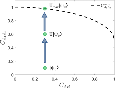
Figure 4: Protocol for quantification of the entanglement between A and B. An initial state $\psi_{0}$ is evolved under a unitary transformation $U$ that acts only on subsystem A, an optimal unitary $U_{max}$ would move the state to the boundary of maximum $C_{A_{1}A_{2}}$. Measurement of $C_{A_{1}A_{2}}$ and the relation on Eq. (10) are then used to quantify $C_{A,B}$.

The protocol just described is an ideal case. In light of the discussions in previous sections, when larger systems are considered, our protocol would require modifications. We identify two challenges that we need to tackle to generate useful insights with this approach. First, for our protocol to work we need a way to quantify either $C_{A_{1},A_{2}}$ or $N_{A_{1},A_{2}}$, however, these quantities are hard to access as we pointed out earlier on. Spin-squeezing parameters could be an interesting candidate to characterize entanglement in spin systems as they involve only the measurement of total spin expectation values, however, even if spin-squeezing parameters can be used to determine whether a system is entangled or not, they cannot generally be used to quantify how much entanglement is present in the system [29].

Second, the relation between the entanglement of A and B and the maximal entanglement that can be generated in A being non-monotonic and widely spread will damage the predictive power of the protocol. Nonetheless, we note that the states shown in Fig. 3, for example, are randomly sampled, on the contrary, if the states we want to characterize are generated from a known family of initial states and then evolved with a known family of unitary transformations with specific symmetries and conserved quantities, then we would expect the relation between the two quantities of interest to become simpler, though it could still be non-monotonic.

In the next couple of sections, we address both of these challenges and show examples on how our protocol can be used effectively.

V Spin-squeezing and entanglement

Spin-squeezed states are great assets in the field of quantum metrology and have been recently realized in a wide range of platforms [45, 46, 47, 48, 49, 50]. Spin-squeezing parameters are strongly connected to the entanglement measures introduced in the initial sections. For instance, in [51] a complete set of spin-squeezing inequalities was provided, and the violation of them signifies a sufficient condition for non-separability. We should note however, that most entanglement criteria defined in terms of spin-squeezing parameters are expected to determine whether a state is entangled or not (related to the PPT criterion) but do not necessarily map the spin-squeezing parameters into other entanglement measures such as concurrence, negativity, etc. That means most of these criteria can not necessarily quantify entanglement properly, except for some special cases [31].

We investigate the relationship between squeezing parameters and linear entropy for different types of states in the following sections. To carry out the analysis, we start by introducing the squeezing operator we will be considering here:

$$\xi^{2}=\frac{4\text{ min}((\Delta J_{\vec{n}_{\perp}})^{2})}{N}\,,$$ (16)

where $N$ is the number of spin 1/2 particles considered, and $J_{\vec{n}_{\perp}}$ is the spin angular momentum operator in the direction $\vec{n}_{\perp}$, which is any direction perpendicular to the mean spin direction $\vec{n}=\langle\vec{J}\rangle/|\langle\vec{J}\rangle|$, with $\langle\vec{J}\rangle=(\langle J_{x}\rangle,\langle J_{y}\rangle,\langle J_{z}\rangle)^{T}$. $\Delta O=\sqrt{\langle O^{2}\rangle-\langle O\rangle^{2}}$ denotes the uncertainty of an operator $O$, and the minimization is carried out with respect to all perpendicular directions $\vec{n}_{\perp}$. This spin-squeezing operator was first introduced by Kitagawa and Ueda [52] and it is the one we will be using throughout the subsequent analysis, for a review of other spin-squeezing operators we refer the reader to [29].

VI Example Spin Systems

In this section, we test the effectiveness of our protocol on spin $1/2$ systems of different sizes. Each one consists of two subsystems A and B with an equal number of qubits. For all cases we consider the system to be initialized in a pure state with all qubits in $\ket{\downarrow}$ state. We first apply a Hamiltonian $H_{AB}$ that creates entanglement between A and B. At each evolution time $t$ we characterize the entanglement between A and B using the linear entropy on Eq. (2), denoted as $S_{L,AB}$. Subsequently, we apply a local Hamiltonian on system A ($H_{A}$) to maximize the spin squeezing inside of it such that the squeezing parameter $\xi^{2}_{A}$ becomes minimal. We study the relation between the above parameters and show that $\text{min}(\xi^{2}_{A})$ can be a good predictor of $S_{L,AB}$ when the appropriate $H_{A}$ is chosen.

In principle, the choice of $H_{AB}$ can be arbitrary and the choice of an optimal $H_{A}$ depends on the specific generated state and can be hard to calculate. Here we focus on some common types of Hamiltonians that can be used to generate spin squeezing and entanglement, including one-axis twisting (OAT), one-axis twisting with transverse field (TF), and two-axis twisting (TAT) [29]:

$$H_{OAT}=\Omega J_{x}^{2},\;H_{TF}=\Omega J_{x}^{2}+\omega J_{z}\,,$$

$$H_{TAT}=\Omega(J_{x}J_{y}+J_{y}J_{x})\,.$$ (17)

For simplicity, we set $\omega=\Omega$ throughout this paper. To obtain some analytical results, we also consider a GHZ Hamiltonian that can create an $N$-body GHZ state:

$$H_{\text{GHZ}}=\Omega\prod_{i}\sigma_{i}^{x}$$ (18)

where $\sigma_{i}^{x}$ is the Pauli-$x$ operator on spin $i$.

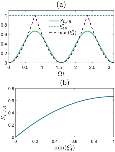
Figure 5: Plots for a 4 qubit system with $H_{AB}$ and $H_{A}$ being a 4-body and 2-body GHZ Hamiltonian, respectively. (a) Linear entropy $S_{L,AB}$ and spin squeezing parameters $\xi_{AB}^{2}$ and $\text{min}(\xi_{A}^{2})$ as a function of $t$. (b) Linear entropy $S_{L,AB}$ as a function of the minimum spin squeezing parameter $\text{min}(\xi_{A}^{2})$ in subsystem A, illustrating a clear monotonic relation.

VI.1 4 qubits with GHZ Hamiltonian

To develop an intuitive understanding, we begin by examining a system composed of four qubits where qubits 1 and 2 constitute subsystem A while qubits 3 and 4 constitute subsystem B. First, we evolve the system with the Hamiltonian defined in Eq. (18) to create entanglement between A and B. We note that the subspace spanned by $\{\ket{0000}\equiv\ket{e_{0}},\ket{1111}\equiv\ket{e_{1}}\}$ is invariant under $H_{AB}$ and since the initial state is taken to be $|\psi_{0}\rangle=|e_{0}\rangle$ we remain in this subspace throughout the evolution. Following the results in previous sections, the states generated under this Hamiltonian should display a monotonic relationship between the bipartite entanglement of A and B and the maximum entanglement that can be generated in A (see purple circles and red dashed line in Fig. 3). The density matrix at time $t$ is given by:

$$\rho_{AB}(t)=\frac{1}{2}\left[\begin{matrix}1+\cos{\left(2\phi\right)}&i\sin{(2\phi})\\ -i\sin{(2\phi})&1-\cos{\left(2\phi\right)}\ \\ \end{matrix}\right],\ \ \phi=\Omega t$$ (19)

Using the definition in Eq.(16), the spin-squeezing parameter is found to be a constant:

$$\xi_{AB}^{2}=1.$$ (20)

The reduced density matrix for subsystem A in the basis $\{\ket{00},\ket{11}\}$ takes the form:

$$\rho_{A}(t)=\frac{1}{2}\left[\begin{matrix}1+\cos{\left(2\phi\right)}&0\\ 0&1-\cos{\left(2\phi\right)}\ \\ \end{matrix}\right]\,.$$ (21)

It follows that we can characterize the entanglement between subsystems A and B using linear entropy as defined in Eq. (2):

$$S_{L,AB}=\frac{2}{3}[1-\cos^{2}{\left(2\phi\right)}]\,.$$ (22)

Now we can fully characterize the system at time $t$, we then consider the application of a local GHZ Hamiltonian $H_{A}=\Omega^{\prime}\sigma_{1}^{x}\sigma_{2}^{x}$ on subsystem A for some time $t^{\prime}$. The spin-squeezing parameter for subsystem A is given by:

$$\xi_{A}^{2}=1-\left|\cos{2\phi}\sin{2\phi^{\prime}}\right|,\;\;\phi^{\prime}=\Omega^{\prime}t^{\prime}\,.$$ (23)

Minimizing $\xi_{A}^{2}$ with respect to $\phi^{\prime}$ to find the optimal evolution time $t^{\prime}$ gives the maximum spin squeezing allowed in subsystem A:

$$\text{min}(\xi_{A}^{2})=1-\left|\cos{2\phi}\right|$$ (24)

Plots of $S_{AB}$, $\xi_{AB}^{2}$, and $\xi_{\text{KU},A,min}^{2}$ as functions of $t$ are shown in Fig. 5(a). The linear entropy in Eq. (22) can be then rewritten in the form:

$$S_{L,AB}=\frac{2}{3}\left[1-\left(1-\text{min}(\xi_{A}^{2})\right)^{2}\right]\,,$$ (25)

which is monotonic for $\text{min}(\xi_{A}^{2})\in[0,1]$ as illustrated in Fig. 5(b). In this simple example, we show that the total spin-squeezing parameter of the system is time-independent so it fails to predict bipartite entanglement between A and B. However, the minimum squeezing parameter for A shows a monotonic relation with the linear entropy, showing a clear advantage of our protocol. For instance, if we are interested in characterizing a state resulting from the evolution under $H_{AB}$ for a time $t$, and we can repeat this state preparation with high accuracy, we might then subsequently evolve with $H_{A}$ for a given time $t^{\prime}$ after which the spin squeezing parameter is determined. By varying $t^{\prime}$ we find the minimum squeezing of $\xi_{A}^{2}$ which can be used to determine $S_{L,AB}$ through Eq. (25). It is in this sense that our protocol utilizes the property of generalized monogamy of entanglement we proposed to quantify the entanglement of A and B.

In terms of efficiency, our protocol still requires the repeated preparation of the state we want to characterize, just as for quantum state tomography. Nonetheless, the number of realizations might be reduced by an efficient choice of the different values of $t^{\prime}$. This could speed up the protocol considerably as long as the profile of $\xi_{A}^{2}(t)$ has some periodicity and not too many local minima.

VI.2 4 and 8 qubit systems with $H_{AB}=H_{OAT}$

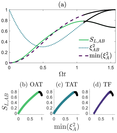
Figure 6: Four-qubit system with $H_{AB}=H_{OAT}$. (a) Linear entropy $S_{L,AB}$ and spin squeezing parameters $\xi_{AB}^{2}$ and $\text{min}(\xi_{A}^{2})$ as a function of time with $H_{A}=H_{TF}$. The section of the dynamics where the one-to-one relation between $\text{min}(\xi_{A}^{2})$ and $S_{L,AB}$ is broken is highlighted with black. The linear entropy $S_{L,AB}$ as a function of minimum spin squeezing parameter $\text{min}(\xi_{A}^{2})$ in subsystem $A$ is shown for (b) $H_{A}=H_{OAT}$, (c) $H_{A}=H_{TAT}$, and (d) $H_{A}=H_{TF}$.

After our discussion in the last section, we now consider a more experimentally relevant case where $H_{AB}=H_{OAT}$. We optimize the spin squeezing in subsystem $A$ with the three Hamiltonians in Eq. (17). The subspace spanned by $\{\ket{e_{0}},\ket{e_{1}}\}$ is no longer preserved by $H_{AB}$, so we study the dynamics numerically. The results are shown in Fig. 6 for a total system of four qubits (two qubits on A and two on B). Since the evolution under $H_{OAT}$ is periodic we only show the evolution of half a period, that is $0\leq\Omega t\leq\pi/2$. For all choices of $H_{A}$, below $S_{AB}\sim 0.6$ there exists a one-to-one relation between $\text{min}(\xi_{A}^{2})$ and $S_{L,AB}$. The similar performances of these Hamiltonians are consistent with the fact that for a subsystem of two qubits, all these Hamiltonians describe very similar dynamics (see Fig. 9 in Appendix B).

The section of the time evolution that breaks the one-to-one relation is highlighted with black in Fig. 6. In this region $\text{min}(\xi_{A}^{2})$ continues to monotonically increase, while $S_{L,AB}$ develops a more complex behavior, which results in a bad accuracy of the protocol for this region. An ideal scenario would be that of the GHZ Hamiltonian case in Fig. 5(a) where both parameters follow the same trends and then the protocol is highly accurate for all ranges of $S_{L,AB}$. To demonstrate why the protocol is failing in this region, we notice that the state at$\Omega t=\pi/2$, where $\text{min}(\xi_{A}^{2})$ becomes maximum but $S_{L,AB}$ reaches a local minimum, is exactly a 4-body GHZ state. Hence the reduced density matrix of subsystem A is a statistical ensemble of state $\ket{00}$ and $\ket{11}$ with equal weights. Due to the special symmetry of a two-qubit system ($J_{x}^{2}=\sigma_{1}^{x}\sigma_{2}^{x}/4$), this state remains invariant under all three $H_{A}$ we chose and no squeezing can be generated using these Hamiltonians ($\text{min}(\xi_{A}^{2})=1$). We note that this might be different from the states with $N_{AB}\geq N_{AB}^{TH}$ in Fig. 3, there, no entanglement in A can be generated with any general unitary operator, here, no further squeezing can be generated with these specific Hamiltonians. Consequently, there might exist some local unitary that further generates squeezing in $A$ [42] for this state, but it can be very difficult to generate the corresponding Hamiltonian.

In more generic circumstances, especially when subsystem A contains more than 2 qubits, one of the three Hamiltonians $H_{A}$ might outperform the others. We illustrate this by applying our protocol in a system of a total of eight qubits with each subsystem containing four of them, the results are presented in Fig. 7.

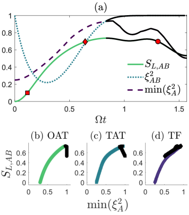
Figure 7: Eight-qubit system with $H_{AB}=H_{OAT}$. (a) Linear entropy $S_{L,AB}$ and spin squeezing parameters $\xi_{AB}^{2}$ and $\text{min}(\xi_{A}^{2})$ as a function of time with $H_{A}=H_{TF}$. Three specific states signaled with square, diamond, and circle markers are selected for further exploration in Fig.8 and are denoted as $p_{1}$, $p_{2}$, and $p_{3}$, respectively. The section of the dynamics where the one-to-one relation between $\text{min}(\xi_{A}^{2})$ and $S_{L,AB}$ is broken is highlighted with black. The linear entropy $S_{L,AB}$ as a function of minimum spin squeezing parameter $\text{min}(\xi_{A}^{2})$ in subsystem $A$ is shown for (b) $H_{A}=H_{OAT}$, (c) $H_{A}=H_{TAT}$, and (d) $H_{A}=H_{TF}$.

The first thing we notice in Fig. 7(a) is that again the linear entropy has a non-monotonic behavior in each period of evolution, however, now we can see that $\text{min}(\xi_{A}^{2})$ develops very similar features when subsystem $A$ is evolved under $H_{A}=H_{TF}$. To visualize this we plot the relation between those two variables in Fig. 7(d) where we see a nearly monotonic relation, which means the optimal squeezing parameter of A would be a good predictor of the bipartite entanglement of A and B. On the contrary, if $H_{A}$ is chosen to be a one- or two-axis twisting Hamiltonian, the relation becomes non-monotonic for highly-entangled states (panels (b) and (c)). Additionally, we see that for both four and eight total qubits, the squeezing parameter of the total system ($\xi_{AB}^{2}$) is a bad predictor of the linear entropy for that state.

VI.3 Effects of different $H_{A}$

The better performance of $H_{A}=H_{TF}$ over the other two options can be understood as follows. Based on the earlier sections, the entanglement between A and B limits the maximum entanglement that can be generated within A, then, the ideal scenario for the proposed protocol is a Hamiltonian $H_{A}$ for which the maximum entanglement within A is reached exactly at the point with the minimal squeezing-parameter.

Let us momentarily focus on subsystem A. We consider three different states generated under $H_{AB}=H_{OAT}$ denoted by red markers in Fig. 7(a). To obtain the value of $\text{min}\left(\xi_{A}^{2}\right)$ we evolve each state with the three possible Hamiltonians $H_{A}$ in Eq. (17) for a long enough time to make sure we explore enough states in the available Hilbert space ($\Omega t=100$). For each point of this evolution, we compute the spin squeezing $\xi_{A}^{2}$ and entanglement negativity $N_{A}$. Note that since the state of $A$ is generally mixed (non-zero bipartite entanglement between A and B) we cannot use linear entropy as a measure of entanglement inside subsystem A.

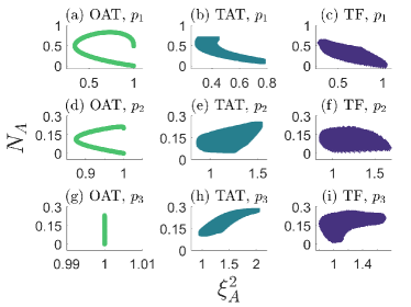
Figure 8: Effects of different $H_{A}$ on capturing maximum entanglement. Three states with different $S_{L,AB}$ are selected from the dynamics under $H_{AB}=H_{OAT}$ and then evolved with three different Hamiltonians $H_{A}$. The negativity of subsystem A is plotted as a function of the total spin squeezing of that subsystem. From left to right the Hamiltonian $H_{A}$ which evolves subsystem A is given by OAT, TAT, and TF, respectively. From top to bottom, the initial mixed state corresponds to $p_{1}$, $p_{2}$, and $p_{3}$, respectively (see Fig.7).

Figure 8 shows the results for states $p_{1}$, $p_{2}$, and $p_{3}$, which correspond to linear entropies $S_{L,AB}=0.1$, $0.7$, and $0.7$, respectively. The difference between $p_{2}$ and $p_{3}$ is that the latter is a state in the non-monotonic regime (see black solid lines in Fig. 7(a)). If we use as a criterion of optimality whether the minimum squeezing is close to the value of maximum entanglement (maximum negativity here), the Hamiltonian $H_{TF}$ is more optimal than the other two for all states. For $p_{3}$ all Hamiltonians perform worse than for $p_{2}$ and $p_{1}$ which is consistent with the results in Fig. 7(b), (c), and (d).

We note that the range of values of squeezing that $H_{A}=H_{OAT}$ can generate, considerably shrinks as the bipartite entanglement $S_{L,AB}$ grows, for state $p_{3}$ almost no squeezing can be generated. $H_{A}=H_{TAT}$, on the contrary, starts to anti-squeeze the spin-ensemble A as the achievable squeezing parameter values start to shift to larger ones. Under the evolution with $H_{A}=H_{TF}$ the general relation between $N_{A}$ and $\xi_{A}^{2}$ is more complex than for the other two, however, it is clear that the smallest spin-squeezing always corresponds to a value of $N_{A}$ that is not too far from the maximum possible value, making it the optimal choice for $H_{A}$ for our protocol.

We emphasize that the latter results are valid given that the states for the composite system A+B are generated under $H_{AB}=H_{OAT}$ and can be understood in terms of conserved symmetries. As we discussed for the point $\Omega t=\pi/2$ in Fig. 6(a), the dynamics might lead to highly symmetric mixed states in A. To squeeze these states further, the breaking of some of those symmetries is required to explore a larger region of the Hilbert space where higher-squeezed states can be reached under the dynamics. For the Hamiltonians in Eq. (17), both $H_{OAT}$ and $H_{TAT}$ are symmetric under the change $\vec{J}\rightarrow-\vec{J}$, additionally, the one-axis twisting Hamiltonian is symmetric for rotations around the $x$-axis while the two-axis twisting Hamiltonian has a discrete symmetry (parity) for rotation around the $z$-axis, namely, $J_{x}\rightarrow-J_{x}$ and $J_{y}\rightarrow-J_{y}$. All of these symmetries are not preserved in $H_{TF}$. Then it is reasonable to deduce that an optimal $H_{A}$ would be a very random-like Hamiltonian where no symmetries are conserved, however, for this work we focused on a family of Hamiltonians that have metrological importance and can be realized in current state-of-the-art experimental platforms.

Numerical simulation of larger spin ensembles can be challenging. Although the initial evolution under $H_{AB}=H_{OAT}$ conserves the total angular momentum $J^{2}$ (the Hilbert space size is linear in $N$), the subsequent evolution under $H_{A}$ breaks this symmetry and the effective Hilbert space size is typically of order $2^{N_{A}}$. However, confirming that the trends in Fig. 8 remain true for larger spin systems would be ideal. In Fig. 9 in Appendix B, we show that, for subsystem A in a pure state, the qualitative features that make $H_{TF}$ the optimal choice, are preserved when subsystem A is increased to have six and eight qubits. Of course, this is still a modest number of qubits, and an experimental implementation of the protocol described here would be the best way to confirm these trends for systems of hundreds or thousands of qubits.

VII Conclusions

We conceptually introduced a protocol to quantify the entanglement in a bipartite system by a subsequent coherent evolution and measurement of one of the subsystems, which was inspired by the generalized monogamy entanglement relations derived at the beginning of the article. We show that in very specific cases, such as in the GHZ Hamiltonian, the protocol works with near-perfect accuracy (would only be limited by experimental errors), while in other more experimentally relevant cases, the accuracy of the protocol can be pushed by an efficient selection of the subsystem Hamiltonian $H_{A}$.

Another advantage of this protocol, besides the challenging techniques required for efficient quantum state tomography, is the fact that entangled subsystems (A and B here) can be separated far apart [53, 54], especially for applications on quantum communication. In that case, only local operations (on a given subsystem) and communication with other parties are available to quantify the entanglement between subsystems, our protocol could then be integrated into these types of applications as it only relies on local unitary evolution and measurement.

Although we only focused on spin systems due to the recent progress in the generation of spin-squeezed states in multiple platforms, the ideas presented here can be extended to heterogeneous systems where spins are coupled to a different set of degrees of freedom. We also emphasize that the results presented are restricted to the case where the total system composed of A and B is in a pure state. In general, mixing of the state would decrease the accuracy of the protocol as now the squeezing of subsystem A can be influenced not only by the bipartite entanglement between A and B but also by the classical correlations of the classical mixture. Nonetheless, given the cleanliness and high control in current experimental platforms, we expect that target entangled states can be generated with a sufficiently low degree of mixing, and consequently, we think this protocol might potentially work to high accuracy in such cases although further numerical exploration to confirm this is pending.

VIII Appendix A: Negativity for $2+N$ systems

For a three-qubit system (two qubits on A and one on B) on a pure state described by (5), the density matrix of the composite system $AB$ can be effectively represented as 4-dimensional matrix on the basis of $\ket{\lambda_{i}}\otimes\ket{\beta_{j}},\;i,j=1,2$:

$$\rho_{AB}=\left[\begin{matrix}\lambda_{1}&0&0&\sqrt{\lambda_{1}(1-\lambda_{1})}\\ 0&0&0&0\\ 0&0&0&0\\ \sqrt{\lambda_{1}(1-\lambda_{1})}&0&0&\lambda_{1}\\ \end{matrix}\right].$$ (26)

Taking partial transpose with respect to subsystem $A$ gives:

$$\rho^{T_{A}}_{AB}=\left[\begin{matrix}\lambda_{1}&0&0&0\\ 0&0&\sqrt{\lambda_{1}(1-\lambda_{1})}&0\\ 0&\sqrt{\lambda_{1}(1-\lambda_{1})}&0&0\\ 0&0&0&1-\lambda_{1}\\ \end{matrix}\right].$$ (27)

By explicitly diagonalizing $\rho^{T_{A}}_{AB}$ we can identify $\lambda_{4}^{T_{A}}=-\sqrt{\lambda_{1}(1-\lambda_{1})}$ as the only possible negative eigenvalue. Substituting this result into the definition of normalized negativity gives us Eq.(11).

Following a similar procedure we can derive the negativity for the system of $2+N$ qubits. In this case, $\rho^{T_{A}}_{AB}$ is given by a $16\times 16$ dimensional matrix that contains six possible negative eigenvalues following the form $(\delta_{ij}-1)\sqrt{\lambda_{i}\lambda_{j}}$, where $i,j=1,2,3,4$, and $\sum_{i=1}^{4}\lambda_{i}=1$. Consequently, the normalized negativity for this case is given by Eq.(15).

IX Appendix B: Role of $H_{A}$ for pure states

In the main text, we found that for the case of four qubits (four on A and four on B) all three $H_{A}$ perform similarly, however, for eight total qubits, $H_{A}=H_{TF}$ performs considerably better than the other two.

Here, to gain some intuition, we study the effect of the choice of $H_{A}$ if subsystem A is considered to be in a pure state with all spins pointing down. Of course, in our protocol, the state of A is mixed (see Fig.8), but considering this simple pure state still allows us to see the trends caused by an increase in the size of A. In Fig.9 we show the relation between linear entropy in A and squeezing in A for two, four, six, and eight qubits composing A (note that here we can use linear entropy as a measure of entanglement as we consider the state to be pure).

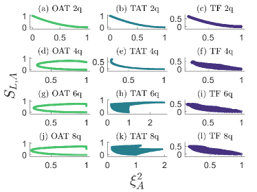
Figure 9: Effects of different $H_{A}$ on capturing maximum entanglement for a pure state. The linear entropy $S_{L,A}$ of subsystem A is plotted as a function of the total spin squeezing of that subsystem. From left to right the Hamiltonian $H_{A}$ which evolves subsystem A is given by OAT, TAT, and TF, respectively, these Hamiltonians are defined in Eq.(17)). From top to bottom, the size of subsystem A varies between two, four, six, and eight qubits.

For A composed of only two qubits, we confirm that all Hamiltonians perform almost identically given the reduced dimensionality of the system, consistent with the results in Fig.6. However, for all system sizes larger than that, $H_{TF}$ becomes more optimal for the protocol as the minimal squeezing in A is closely related to the maximum entanglement within A. Moreover, we see that the general features of the action of $H_{TF}$ seem to be very robust to increasing the system size making it reasonable to consider that this Hamiltonian will still be the optimal choice for larger systems.