Bayesian Perspective for Orientation Estimation in Cryo-EM and Cryo-ET

Abstract

Accurate orientation estimation is a crucial component of 3D molecular structure reconstruction, both in single-particle cryo-electron microscopy (cryo-EM) and in the increasingly popular field of cryo-electron tomography (cryo-ET). The dominant method, which involves searching for an orientation with maximum cross-correlation relative to given templates, falls short, particularly in low signal-to-noise environments. In this work, we propose a Bayesian framework to develop a more accurate and flexible orientation estimation approach, with the minimum mean square error (MMSE) estimator as a key example. This method effectively accommodates varying structural conformations and arbitrary rotational distributions. Through simulations, we demonstrate that our estimator consistently outperforms the cross-correlation-based method, especially in challenging conditions with low signal-to-noise ratios, and offer a theoretical framework to support these improvements. We further show that integrating our estimator into the iterative refinement in the 3D reconstruction pipeline markedly enhances overall accuracy, revealing substantial benefits across the algorithmic workflow. Finally, we show empirically that the proposed Bayesian approach enhances robustness against the “Einstein from Noise” phenomenon, reducing model bias and improving reconstruction reliability. These findings indicate that the proposed Bayesian framework could substantially advance cryo-EM and cryo-ET by enhancing the accuracy, robustness, and reliability of 3D molecular structure reconstruction, thereby facilitating deeper insights into complex biological systems.

1 Introduction

Determining the precise three-dimensional (3D) orientation of biological molecules from their noisy two-dimensional (2D) projection images is a fundamental challenge in cryo-electron microscopy (cryo-EM) [1, 30, 37, 7]. This process, known as orientation estimation, is crucial for various cryo-EM applications, including 3D reconstruction algorithms [44, 40], heterogeneity analysis [51, 55, 13, 63], and beyond [32]. Figure 1(a) illustrates the role of orientation estimation within the cryo-EM 3D reconstruction workflow.

In cryo-electron tomography (cryo-ET), orientation estimation presents an additional challenge in the form of subtomogram averaging. Notably, cryo-ET suffers from higher noise levels compared to single-particle cryo-EM due to the complex and heterogeneous nature of cellular samples and the challenges of capturing data from multiple angles within thicker specimens. Subtomogram averaging offers an effective approach to enhance the signal-to-noise ratio (SNR), ultimately resulting in the reconstruction of high-resolution structures. This technique often involves extracting multiple similar subtomograms containing the target protein complex or macromolecule from a large cryo-electron tomogram reconstructed from all available tilts (typically from $-60^{\circ}$ to $+60^{\circ}$), followed by aligning and averaging them [61, 58]. Unlike traditional cryo-EM, this process typically aligns 3D structures directly, without the direct use of 2D projections (see Figure 1(b) for an illustration).

Mathematically, the orientation estimation tasks in cryo-EM and cryo-ET are slightly different. In the process of cryo-EM, which involves 2D tomographic projections, the mathematical model can be formulated as:

$$y=\Pi(g^{-1}\cdot V)+\varepsilon,$$ (1.1)

where $y$ is the observed 2D projection image, $V$ is the underlying 3D molecular structure, $\Pi$ is the tomographic projection operator, $g$ is the unknown 3D rotation operator of interest, $\varepsilon$ represents measurement noise, and $g^{-1}\cdot V(x)\equiv V(gx)$, representing a rotation acting on a volume $V$ with 3D coordinate $x$. Analogously, the mathematical model in cryo-ET subtomogram averaging, which aligns directly with the 3D structure, can be represented by:

$$y=g^{-1}\cdot V+\varepsilon,$$ (1.2)

where $y$ is the observed 3D subtomogram, $V$ is the underlying 3D molecular structure, $g$ is the unknown 3D rotation operator of interest, and $\varepsilon$ represents measurement noise. Then, the goal of orientation estimation is to find the “best” 3D rotation $g$ based on the 2D projection image (in the cryo-EM case (1.1)) or the 3D subtomogram (in the cryo-ET case (1.2)) with respect to the 3D reference $V$. Namely, we aim to estimate the rotation $g$ given the sample $y$ and the 3D structure $V$.

While this work focuses on 3D rotation estimation, its methodology and results can be readily extended to various other transformations, including translations and permutations; we will discuss this further in Section 5.

1.1 The gap

The common approach to estimating a rotation from an observation in the models above involves scanning through a pre-defined set of possible rotations and selecting the one that either maximizes the correlation or minimizes the distance to the given reference (2D projection image or 3D molecular structure, depending on the application). From the perspective of Bayesian statistics, this process corresponds to the maximum a posteriori (MAP) estimator, assuming a uniform prior over all the orientations (namely, all orientations are a priori equally likely). Therefore, we refer to this estimator as the MAP estimator in the sequel. However, Bayesian theory provides a much deeper and richer statistical framework that leads to improvement: replacing the MAP estimator with the Bayes estimator. The full potential of this estimator—that provides optimal accuracy according to a user-defined loss function and allows for integrating prior knowledge about rotational distributions—remained untapped so far.

The term rotational distribution broadly describes how rotations are distributed probabilistically over all possible orientations in 3D space. In cryo-electron microscopy, this concept becomes particularly relevant. During sample preparation, proteins are embedded in a thin layer of vitreous ice. Ideally, these proteins would adopt completely random orientations, resulting in what mathematicians refer to as a uniform distribution over the rotation group. In our model (1.1) or (1.2), this corresponds to the underlying prior distribution of the rotation $g$. This randomness is often assumed in modeling, as it simplifies analysis and reflects the desired experimental setup. However, in practice, proteins frequently display preferred specimen orientations due to interactions with the ice or other factors, leading to a distribution that is not uniform [53, 30, 29]. This means that some orientations are more likely than others, which has important implications for the methodologies employed in orientation estimation.

Currently, the vast majority of cutting-edge software for 3D structure reconstruction, e.g., RELION [44] and cryoSPARC [40], outputs the MAP orientation estimator. Although these tools are primarily designed for 3D structure reconstruction and treat rotation estimation as a nuisance problem, researchers may inadvertently use these orientation estimates for downstream tasks, potentially leading to suboptimal results. This work explores opportunities to improve orientation estimation, especially in low SNR conditions where the MAP estimator performs poorly.

1.2 The Bayesian framework

The Bayesian framework has become a powerful and widely adopted tool in cryo-EM, now recognized as the leading method for recovering 3D molecular structures [44, 40, 55, 15]. It effectively addresses challenges like overfitting and parameter tuning while enhancing interpretability [43]. By explicitly modeling uncertainties, Bayesian methods enable more accurate and robust reconstructions of molecular structures, driving significant advances in both resolution and structural flexibility. While the majority of these methods focus on the task of structure reconstruction (e.g., see model (4.1)) and aim to achieve the MAP estimator for the volume structure [44, 40], the Bayesian framework offers broader possibilities for addressing other problems.

In this work, we propose a versatile Bayesian framework specifically for orientation estimation, which has superior statistical properties and is highly flexible. This framework enables the use of any loss function over the rotational group tailored to users’ requirements and accommodates a broad range of prior distributions, beyond the uniform distribution. In particular, while the Bayesian framework can be adapted to different loss functions, this work focuses on the mean-squared error (MSE) loss, which is equivalent to the chordal distance between 3D rotations. The primary reason for using this loss function is that its corresponding Bayes estimator has a closed-form analytical solution, making it computationally efficient and easy to interpret. We denote this estimator as $\hat{g}_{\text{MMSE}}$, where MMSE stands for minimum mean square error. It is worth noting that for any given loss function and prior distribution, the Bayes estimator is optimal among all possible estimators. Moreover, the computational cost of calculating our $\hat{g}_{\text{MMSE}}$ estimator is at the same scale as that of the commonly used MAP orientation estimator (See Section 3 for more details).

Figure 1 illustrates the critical role of orientation estimation in the cryo-EM and cryo-ET reconstruction processes, showcasing the superior performance of the MMSE orientation estimator, $\hat{g}_{\text{MMSE}}$, compared to the MAP orientation estimator, $\hat{g}_{\text{MAP}}$. Specifically, the curves show that the MMSE estimator consistently produces more accurate estimates than the MAP estimator, with the performance gap widening as the SNR decreases. Moreover, incorporating prior knowledge of rotational distribution into our MMSE estimator allows for even better performance (See Figure 2). This performance gap becomes even more pronounced when the estimators are incorporated into a reconstruction algorithm (see Section 4).

The main takeaway of this paper is the recommendation to use the Bayesian MMSE orientation estimator to determine the orientation of each observation, in place of the commonly used MAP orientation estimator. The MMSE estimator demonstrates superior performance even under a uniform distribution, with the potential for further significant improvements when leveraging knowledge of underlying rotational distribution. Since the MMSE estimator for orientation determination is already integrated into many software packages, this adjustment should be easy to implement with minimal additional computational cost.

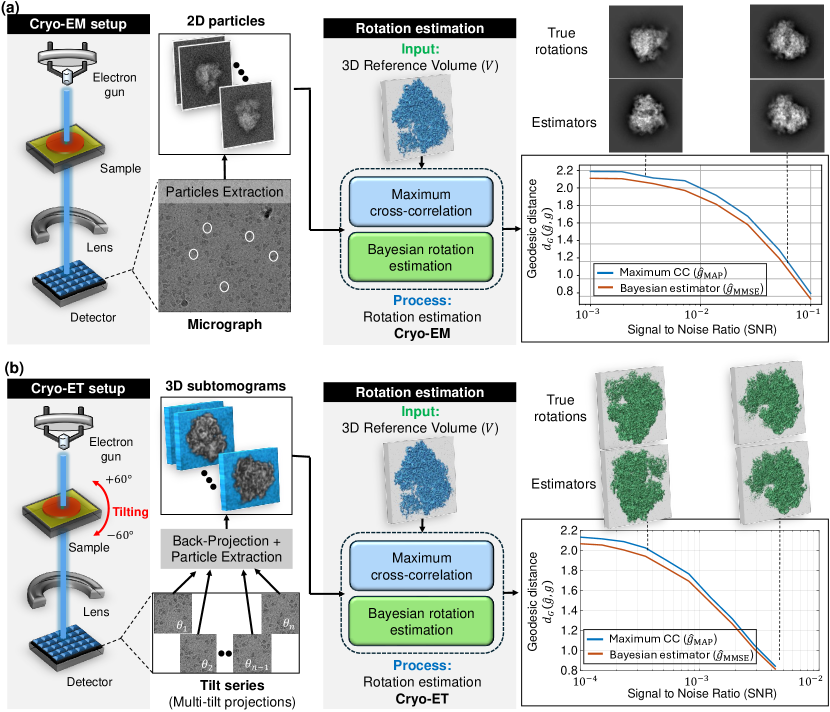
Figure 1: Comparison between maximum cross-correlation ($\hat{g}_{\text{MAP}}$) and Bayesian ($\hat{g}_{\text{MMSE}}$) orientation estimators in cryo-electron microscopy (cryo-EM) and cryo-electron tomography (cryo-ET) applications. The figure illustrates the general workflow in cryo-EM and cryo-ET techniques, highlighting the role of orientation estimation in each technique. Panel (a) illustrates the model with 2D projections (cryo-EM model, (1.1)), while panel (b) shows the model without projections (cryo-ET model, (1.2)). (a) Cryo-EM involves imaging macromolecules embedded in a thin layer of vitreous ice using an electron beam in a transmission electron microscope (TEM). The process generates 2D projection images (micrographs) of particles in unknown 3D orientations. These 2D particles are then identified and extracted from the micrographs, forming the basis for subsequent steps of the macromolecule’s 3D structure reconstruction. (b) Cryo-ET involves imaging a sample from multiple known tilt angles (typically from $-60^{\circ}$ to $+60^{\circ}$) to create 2D projections, which are then combined computationally to reconstruct 3D subtomograms. In this context, a subtomogram refers to a small volume containing an individual 3D particle. The subtomograms are extracted by a particle picker algorithm for further analysis. (a+b): The rotation estimation problem involves determining the relative orientation of a noisy 2D particle (in cryo-EM) or a noisy 3D subtomogram (in cryo-ET) relative to a reference volume $V$. The reference volume structure used in both setups is identical and corresponds to the 80S ribosome [59]. Under high SNR conditions, both rotation estimators closely approximate the true relative rotation. However, as the SNR decreases, the estimation accuracy declines. Importantly, across all SNR levels, the geodesic angular distance between the MMSE orientation estimator and the true rotation consistently remains lower than that of the MAP orientation estimator. For (a), the estimation was conducted using a grid size of $L=3000$ samples of the rotation group $\mathsf{SO}(3)$, while for (b), a grid size of $L=300$ was used. Each point in the two curve plots represents the average error computed over 3000 trials.

1.3 Overview of results and contributions

Section 2 details the mathematical model and Bayesian approach, focusing on the MMSE estimator. The theoretical result examines the MMSE estimator’s behavior, explaining why it performs similarly to the MAP estimator in high-SNR conditions (Proposition 2.1), while consistently outperforming it in low-SNR conditions (Figure 1)—a frequent scenario in cryo-EM and cryo-ET applications [7].

Section 3 presents numerical simulations evaluating the performance of the MMSE estimator. These simulations explore the effects of various prior distributions on rotations and the influence of the sampling grid resolution, denoted as $L$, within the rotation group $\mathsf{SO}(3)$. Here, $\mathsf{SO}(3)$ refers to the special orthogonal group in three dimensions, representing the set of all possible 3D rotations. The parameter $L$ determines the granularity of the discretization applied to $\mathsf{SO}(3)$ in these simulations. We highlight that incorporating non-uniform prior distributions on rotations significantly improves estimation accuracy, emphasizing the importance of the prior information of rotational distribution and offering promising avenues for future integration within cryo-EM and cryo-ET frameworks (Figure 2). Moreover, empirical results show that in high-SNR conditions, the distance between the estimators and the true rotation scales proportionally to $L^{1/3}$ (Figure 3), whereas this effect diminishes in low-SNR conditions.

In Section 4, the MMSE estimator is connected to the orientation estimation step in 3D reconstruction algorithms (for models without projections), where soft-assignment methods are used. This connection demonstrates that incorporating the MMSE estimator into reconstruction algorithms is equivalent to the widely used expectation-maximization (EM) algorithm [46] (Proposition 4.1). Our experiments clearly show that both 2D and 3D reconstructions using the MMSE estimator significantly outperform those using the MAP estimator (Figures 4 and 5). Notably, the MMSE estimator demonstrates robustness against the “Einstein from Noise” phenomenon [19, 3], with empirical evidence showing reduced bias in 3D reconstruction (Figures 4 and 5). Section 5 summarizes the results and delineates future research directions.

1.4 Related Works

Estimating rotations in cryo-EM and cryo-ET involves two distinct but related tasks: 3D alignment and synchronization.

3D Alignment techniques.

3D alignment, which is a key focus of this work, aims to determine the relative orientation between two 3D volumes (in cryo-ET) or to estimate the orientation associated with a projection image (in cryo-EM). 3D alignment is often achieved through cross-correlation techniques, such as the MAP estimator. This task is commonly applied for downstream analysis or for comparing different conformational states.

Various alignment methods have been proposed in the literature. For instance, the Xmipp software package provides a 3D alignment algorithm based on spherical harmonics expansion and fast rotational matching [11]. The EMAN2 software package offers two 3D alignment methods: one that estimates rotation via an exhaustive Euler angle search with iterative angular refinement, and a more efficient tree-based approach that performs hierarchical 3D alignment with progressively finer downsampling in Fourier space [54]. Another approach is the projection-based volume alignment algorithm, which matches projections of the two volumes [60]. In [17], the authors propose leveraging common lines between projection images of the maps. Additionally,  [50] suggests that replacing the traditional Euclidean distance with the 1-Wasserstein distance creates a smoother optimization landscape and a larger basin of attraction.

Synchronization.

In contrast to 3D alignment, synchronization aims to recover a set of rotations from their corresponding rotated measurements without accessing the ground truth volumes. The standard approach follows a two-stage process: (1) estimating the relative rotation between each pair of observations; and (2) inferring global rotations from these pairwise ratios. The main techniques in this area rely on spectral decomposition [47], message passing [39], and convex optimization [5]. These methods have been applied to estimate projection orientations in cryo-EM, where the relative rotations between projections are determined using the common-lines property [56, 45, 49]. Recently, new deep learning-based methods have been developed for this task [36, 38, 24].

Rotationally invariant techniques.

It is worth noting that the unknown rotations in cryo-EM and cryo-ET are sometimes treated as nuisance parameters. This is because rotation estimation is often an intermediate step, with the primary goal being the estimation of the 3D structure itself. Consequently, some methods aim to estimate the 3D structure (or images) directly by leveraging features, such as polynomials, that are invariant to rotations (or translations). For example, in [62, 31], the bispectrum of images was used for rotationally invariant clustering. Similar techniques based on the method of moments have also been applied to 3D reconstruction; see, for example, [28, 8].

2 Problem formulation and the MMSE orientation estimator

In this section, we present a particular Bayes estimator, the minimum mean square error (MMSE) estimator, for orientation determination within the Bayesian framework. We begin by introducing a flexible mathematical model that encompasses various typical applications involving orientation estimation. Following this, we present a couple of metrics designed to assess the quality of our estimators, providing a robust framework for evaluating performance. Finally, we introduce the class of Bayes estimators, with the MMSE estimator serving as a primary example.

Throughout this paper, we use $g$ to denote both the rotation operator and its corresponding matrix representation. For instance, $g$ can be represented by a $3\times 3$ rotation matrix in 3D. The intended meaning will be clear from the context, and this slight abuse of notation should not cause confusion.

2.1 Mathematical model for orientation estimation

Let $V(x):\mathbb{R}^{n}\to\mathbb{R}$ be a structure that represents the reference projection $(n=2)$ or volume $(n=3)$, and let $\mathsf{G}$ be the group of 2D or 3D rotations correspondingly. For example, when $n=3$, $V$ corresponds to the continuous 3D electron density, as commonly used in cryo-EM or cryo-ET. We emphasize that the methodology can be readily extended to any compact group, which is a subgroup of the orthogonal group in $\mathbb{R}^{n}$; a notable example is the group of circular shifts [9]. Let $\Pi$ be a known linear operator comprising the discretization sampling operator and potentially a tomographic projection operator. We thus model a single measurement $y$ as

$$y=\Pi(g^{-1}\cdot V)+\varepsilon\in\mathbb{R}^{d},$$ (2.1)

where $d$ is the total dimension of measurement space, $g\sim\Lambda$ is an unknown random element of $\mathsf{G}$ following a possibly non-Haar (i.e., non-uniform) distribution $\Lambda$ over $\mathsf{G}$, and $\varepsilon\sim\mathcal{N}(0,\sigma^{2}I_{d\times d})$ is the standard Gaussian measurement noise vector with zero mean and variance level of $\sigma^{2}$. For simplicity, we omit $\Pi$ when it only represents the discretization sampling operator.

Modeling structural uncertainty.

In real-world scenarios, particles infrequently conform to an exact, uniform structure. Instead, they often exhibit slight variations due to different deformations or conformational changes (e.g., [55]). To capture this inherent variability, we introduce a more nuanced model for the volume. Rather than assuming a fixed structure, we represent the volume with a mean $\overline{V}$ and incorporate uncertainty through a diagonal covariance matrix $\Sigma=\operatorname{diag}(\tau_{1}^{2},...,\tau_{d}^{2})$. This covariance matrix can be obtained by discretizing the covariance structure of a pre-specified isotropic Gaussian process $W$ in the $d$ dimensional measurement space, where this Gaussian process reflects the user’s assumptions or understanding of structural uncertainty. The isotropy assumption reflects the idea that structural variations are equally likely in all directions. In other words, we assume $V$ has the following flexible structure

$$V(x)\mathrm{d}x=\overline{V}(x)\mathrm{d}x+\mathrm{d}W(x),~{}\text{ for }~{}x\in\mathbb{R}^{3},$$ (2.2)

where $\overline{V}$ is a given mean function, and $W$ is a given isotropic Gaussian process over $\mathbb{R}^{3}$, representing possible local conformation differences between $V$ and $\overline{V}$. Here, isotropic means that its statistics remain invariant under rotations; that is, for any $g\in\mathsf{G}$, we have $W(gx)=W(x)$. Combining (2.1) and (2.2) yields the simplified model

$$y=\Pi(g^{-1}\cdot\overline{V})+\overline{\varepsilon}+\varepsilon\in\mathbb{R}^{d},$$ (2.3)

where $\overline{\varepsilon}\sim\mathcal{N}(0,\mathrm{diag}(\tau_{1}^{2},\ldots,\tau_{d}^{2}))$ with a known variance structure.

Applications of the model.

We present three typical examples of this model. In all cases, the goal is to estimate $g$ given the sample $y$, the structure $\overline{V}$, and the noise levels $\sigma^{2}$ and $\{\tau_{1}^{2},\ldots,\tau_{d}^{2}\}$.

1. 2D template matching. In this case, $\Pi$ is solely the discretization sampling operator, $d=N\times N$ with $N$ the grid size of 2D projection images, $g\in\mathsf{G}=\mathrm{SO}(2)$ is a 2D in-plane rotation, and $\overline{V}$ is a given 2D template image. Here, $V$ represents a noisy version of $\overline{V}$, potentially corrupted due to averaging or other pre-processing procedures.

2. Rotation estimation in cryo-EM. Here, we consider a special case of (2.3) where $\Pi$ comprises both the sampling and tomographic projection operators, $d=N\times N$ with $N$ the grid size of 2D projection images, $g\in\mathsf{G}=\mathsf{SO}(3)$ is a 3D rotation, and $\overline{V}$ is a given 3D volume representing a known reference 3D structure or a well-grounded structure from prior data analyses.

3. 3D structure alignment in cryo-ET. In this scenario, we consider a special case of (2.3) where $\Pi$ is solely the discretization sampling operator, $d$ corresponds to the total dimension of 3D subtomograms, $g\in\mathsf{G}=\mathsf{SO}(3)$ is a 3D rotation, and $\overline{V}$ is a given 3D volume. Notably, the 3D alignment problem is also a critical step in the computational pipeline of cryo-EM, see, e.g., [50, 17].

Metrics over SO(3).

As the MMSE estimator is tightly related to given loss functions, we present two candidate metrics over the 3D orthogonal group $\mathsf{SO}(3)$. It is important to note that our framework is flexible and can accommodate other loss functions over any group $\mathsf{G}$. For a more comprehensive discussion on metrics for rotations, we direct readers to the works of [18, 21]. While similar metrics and estimation procedures apply to the $\mathrm{SO}(2)$ estimation problem, we omit detailed discussion for brevity.

1. Chordal distance. For any two rotations $g_{1},g_{2}\in\mathsf{SO}(3)$, the chordal distance is defined as

   $$d_{F}(g_{1},g_{2})\triangleq\|g_{1}-g_{2}\|_{F}=\sqrt{\mathrm{tr}\Big{(}{\left(g_{1}-g_{2}\right)^{\mathsf{T}}\left(g_{1}-g_{2}\right)}\Big{)}},$$ (2.4)

   where $\left\|\cdot\right\|_{F}$ represents the matrix Frobenius norm, and $\mathrm{tr}(\cdot)$ is the trace of a matrix. This metric is easy to compute and analyze, however, it does not take into account the group structure of rotations.

2. Geodesic distance. For any two rotations $g_{1},g_{2}\in\mathsf{SO}(3)$, the geodesic distance is defined as

   $$d_{G}(g_{1},g_{2})\triangleq\arccos\left(\frac{\mathrm{tr}(g_{2}g_{1}^{-1})-1}{2}\right),$$ (2.5)

   where $\mathrm{tr}(\cdot)$ is the trace of a matrix. This metric reflects the shortest path between $g_{1}$ and $g_{2}$ over the manifold of 3D rotations.

2.2 The MMSE and MAP orientation estimators

Before introducing the specific estimator for our model (2.3), it is instructive to briefly revisit the general Bayesian framework and the concept of the Bayes estimator. This will provide the necessary foundation for understanding the development and analysis of our proposed MMSE estimator, as well as its superior statistical properties compared to the widely used MAP estimator.

Overview of Bayesian framework and the Bayes estimator.

Suppose we aim to estimate some true rotation $g\in\mathsf{G}$ drawn from a known prior distribution $\Lambda$ from data. Let $\hat{g}$ be an estimator of $g$ based on a measurement $y$ and let $\mathcal{L}\left(g,\hat{g}\right)$ be a loss function (for example, the chordal and geodesic distances). The Bayes risk of $\hat{g}$ is defined as $\mathbb{E}_{\Lambda}[\mathcal{L}\left(g,\hat{g}\right)]$, where the expectation is taken over the data generating process of $y$ given $g$ and the prior distribution $\Lambda$ of $g$. The Bayes estimator [27, Chapter 4, Theorem 1.1] is defined as the estimator that minimizes the Bayes risk among all estimators, i.e.,

$$\hat{g}_{\mathsf{Bayes}}=\underset{\hat{g}}{\operatorname*{arg\,min}}\ {\mathbb{E}_{\Lambda}\left[\mathcal{L}\left(g,\hat{g}\right)\right]}.$$ (2.6)

Equivalently, it is the estimator that minimizes the posterior expected loss $\mathbb{E}_{\Lambda}[\mathcal{L}\left(g,\hat{g}\right)|y]$, where the expectation is taken over the posterior distribution of $g$ given the measurement $y$, and the known volume $\overline{V}$, with the prior $\Lambda$, i.e.,

$$\hat{g}_{\mathsf{Bayes}}=\underset{\hat{g}}{\operatorname*{arg\,min}}\ \mathbb{E}_{\Lambda}\left[\mathcal{L}\left(g,\hat{g}\right)|y,\overline{V}\right],$$ (2.7)

with

$${\mathbb{P}}_{\Lambda}(g|y,\overline{V})\mathrm{d}g=\frac{{\mathbb{P}}(y|g)\mathrm{d}\Lambda(g)}{\int_{\mathsf{G}}{\mathbb{P}}(y|g)\mathrm{d}\Lambda(g)}.$$

The posterior distribution of the rotation $g$ given the observation $y$ under model (2.3).

To introduce the MMSE estimator corresponding to the model (2.3), we first compute the posterior distribution of $g$ given $y$ and all the additional parameters $\overline{V}$, $\sigma^{2}$ and $\{\tau_{1}^{2},\ldots,\tau_{d}^{2}\}$. We can rewrite (2.3) as

$$y= \Pi(g^{-1}\cdot\overline{V})+\bar{\varepsilon}+\varepsilon=\Pi(g^{-1}\cdot\overline{V})+\tilde{\varepsilon},$$ (2.8)

where $\tilde{\varepsilon}:=\bar{\varepsilon}+\varepsilon\sim\mathcal{N}(0,\tilde{\Sigma})$ with $\tilde{\Sigma}=\mathrm{diag}(\tilde{\tau}_{1}^{2},\ldots,\tilde{\tau}_{d}^{2})$ and $\tilde{\tau}_{i}^{2}=\tau_{i}^{2}+\sigma^{2}$. Therefore, we obtain the conditional likelihood density

$${\mathbb{P}}(y|g,\overline{V})=\frac{1}{(2\pi)^{d/2}\mathrm{det}(\tilde{\Sigma})^{1/2}}\exp\Big{(}-\frac{1}{2}(y-\Pi(g^{-1}\cdot\overline{V}))^{\mathsf{T}}\tilde{\Sigma}^{-1}(y-\Pi(g^{-1}\cdot\overline{V}))\Big{)}.$$

Note that $g$ has the prior distribution $\Lambda$. Applying the Bayes’ law, the posterior distribution of $g$ given $y$ is

$${\mathbb{P}}(g|y,\overline{V})\mathrm{d}g=\frac{\exp\Big{(}-\frac{1}{2}(y-\Pi(g^{-1}\cdot\bar{V}))^{\mathsf{T}}\tilde{\Sigma}^{-1}(y-\Pi(g^{-1}\cdot\overline{V}))\Big{)}\mathrm{d}\Lambda(g)}{\int_{\mathsf{G}}\exp\Big{(}-\frac{1}{2}(y-\Pi(g^{-1}\cdot\overline{V}))^{\mathsf{T}}\tilde{\Sigma}^{-1}(y-\Pi(g^{-1}\cdot\overline{V}))\Big{)}\mathrm{d}\Lambda(g)}.$$ (2.9)

The MAP estimator.

Recalling the maximum cross-correlation method we mentioned earlier, we now connect it with our mathematical model (2.8) and introduce the corresponding MAP estimator. Assume, in this explicit model with $\mathsf{G}=\mathsf{SO}(3)$, $\Lambda$ is the uniform distribution and all $\tilde{\tau}_{i}$’s are equal to $\tilde{\tau}$. Then, the rotation $g$ that minimizes the distance between the corresponding projected rotated volume $\Pi(g^{-1}\cdot\bar{V})$ and the observation $y$ is exactly the maximum a posteriori (MAP) estimator defined as

$$\hat{g}_{\mathsf{MAP}}:= \operatorname*{arg\,max}_{g\in\mathsf{SO}(3)}{\mathbb{P}}(g|y,\bar{V})$$

$$= \operatorname*{arg\,max}_{g\in\mathsf{SO}(3)}\exp\Big{(}-\|y-\Pi(g^{-1}\cdot\overline{V})\|^{2}/2\tilde{\tau}^{2}\Big{)}$$

$$= \operatorname*{arg\,min}_{g\in\mathsf{SO}(3)}\|y-\Pi(g^{-1}\cdot\overline{V})\|^{2},$$ (2.10)

where the first equality holds because the denominator in (2.9) does not depend on $g$, and additionally, $\Lambda$ is the uniform distribution and $\tilde{\Sigma}=\tilde{\tau}^{2}I_{d\times d}$ for the numerator. In absence of the tomographic projection (e.g., in cryo-ET), the MAP estimator further simplifies to

$$\hat{g}_{\mathsf{MAP}}=\operatorname*{arg\,max}_{g\in\mathsf{SO}(3)}y^{\mathsf{T}}(g^{-1}\cdot\overline{V}),$$

which corresponds to the rotation $g$ such that the rotated structure maximizes the correlation with $y$. This estimator is also frequently used in cryo-EM, under the assumption that the norm of $\Pi(g^{-1}\cdot\overline{V})$ is approximately constant for all $g$. This estimator can be approximated by performing a search over a pre-defined grid of 3D rotations, selecting the rotation that minimizes the distance between the measurement $y$ and the projected rotated volume $\Pi(g^{-1}\cdot\overline{V})$. This approach forms the basis of standard practices in cryo-EM and cryo-ET.

The MMSE estimator.

For any general rotational distribution $\Lambda$, general variance structure of $\tilde{\varepsilon}$, and loss function $\mathcal{L}(\cdot,\cdot)$ over $\mathsf{SO}(3)$, the MAP estimator can be further improved by the corresponding Bayes estimator which minimizes the posterior expected loss $\mathbb{E}_{\Lambda}[\mathcal{L}(g,\cdot)|y,\overline{V}]$. In particular, following the definition (2.7) of the Bayes estimator, and for the chordal distance (2.4), where $\mathcal{L}(\cdot,\cdot)=d_{F}^{2}(\cdot,\cdot)$, the Bayes estimator is equivalent to the MMSE estimator [27, Chapter 4, Corollary 1.2] :

$$\hat{g}_{\mathsf{MMSE}}:= \underset{\hat{g}}{\operatorname*{arg\,min}}\ \mathbb{E}_{\Lambda}\left[d_{F}^{2}\left(g,\hat{g}\right)|y,\overline{V}\right]=\mathbb{E}_{\Lambda}[g|y,\overline{V}]$$

$$= \frac{\int_{\mathsf{SO}(3)}g\exp\Big{(}-\frac{1}{2}(y-\Pi(g^{-1}\cdot\overline{V}))^{\mathsf{T}}\tilde{\Sigma}^{-1}(y-\Pi(g^{-1}\cdot\overline{V}))\Big{)}\mathrm{d}\Lambda(g)}{\int_{\mathsf{SO}(3)}\exp\Big{(}-\frac{1}{2}(y-\Pi(g^{-1}\cdot\overline{V}))^{\mathsf{T}}\tilde{\Sigma}^{-1}(y-\Pi(g^{-1}\cdot\overline{V}))\Big{)}\mathrm{d}\Lambda(g)},$$ (2.11)

where the expectation is taken over the posterior density (2.9). Notably, $\hat{g}_{\mathsf{MMSE}}$ may not be a valid rotation operator in general. Thus, we use the orthogonal Procrustes procedure to obtain a valid rotation, as discussed next. We refer to the estimator obtained through this procedure also as $\hat{g}_{\mathsf{MMSE}}$, provided it causes no misunderstanding. We summarize the numerical procedure for calculating the MMSE estimator for rotation estimation in Algorithm 1.

Orthogonal Procrustes.

It is important to note that $\hat{g}_{\mathsf{MMSE}}$, as defined in (2.11), is not necessarily a valid operator in $\mathsf{SO}(3)$. Consequently, to obtain a valid rotation operator, given a matrix $A$, the objective is to find a matrix representation $\Omega\in\mathsf{SO}(3)$ that is closest to matrix $A$ in terms of the Frobenius norm metric by solving

$$\underset{\Omega}{\text{minimize}}\quad\|\Omega-A\|_{F}\quad\text{subject to}\quad\Omega\in\mathsf{SO}(3).$$ (2.12)

This problem is called the Orthogonal Procrustes in the linear algebra literature and it solved efficiently by singular value decomposition (SVD) of the matrix $A$ [16]. In particular, given the SVD of $A$, represented by $U\Sigma V^{\mathsf{T}}$, the solution can be expressed as $U\Sigma^{\prime}V^{\mathsf{T}}$, where $\Sigma^{\prime}$ is derived from $\Sigma$ by setting the smallest singular value to $\det(UV^{\mathsf{T}})$ and all other singular values to 1, so that the determinant of the solution is guaranteed to be positive as desired.

The MMSE and MAP estimators in the high SNR regime.

The next proposition shows that the MMSE and MAP estimators converge in the high SNR regime (i.e., $\sigma\to 0$), as demonstrated empirically in Figures 3, 4, and 5. This implies that the MMSE estimator’s superior statistical properties are most advantageous in low SNR conditions, which are common in structural biology applications like cryo-EM and cryo-ET [7]. In these low SNR environments, the MMSE estimator consistently outperforms its MAP counterpart. Assume $\tau_{i}^{2}=0$ as part of the model introduced in (2.3). Thus, the noise covariance matrix is given by $\Sigma=\sigma^{2}I_{d\times d}$. In the following sections, we maintain this setting for simplicity, as it is sufficient to convey our main arguments.

Proposition 2.1.

Let $\hat{g}_{\mathrm{MAP}}$ be the MAP rotation estimator as defined in (2.10), and assume it is unique. Let $\hat{g}_{\mathrm{MMSE}}$ be the MMSE estimator as defined in (2.11), where $\Lambda$ is a uniform measure over $\mathsf{SO}(3)$. Then,

$$\lim_{\sigma\to 0}\hat{g}_{\mathrm{MMSE}}=\hat{g}_{\mathrm{MAP}}.$$ (2.13)

The proof of the proposition is provided in Appendix A. The proof relies on the existing result, [41, Theorem 5.10], and is valid not only to rotations but also to other group operators, such as translations.

3 Numerical methods for MMSE orientation estimation

This section compares the numerical performance of the MMSE and MAP estimators. We introduce various types of prior distributions for $\mathsf{SO}(3)$ beyond the uniform distribution and demonstrate how incorporating this prior knowledge can significantly improve the performance of the MMSE rotation estimator. Furthermore, we study the influence of the number of sampling points of the group $\mathsf{SO}(3)$ of 3D rotations (namely, the number of candidate rotations), denoted as $L$, on the quality of rotation estimation. For better illustration, we consider the simplified setting of model (2.3), where we assume $\tau_{i}^{2}=0$ for all $i$, which means $\tilde{\Sigma}=\sigma^{2}I_{d\times d}$ in (2.9).

Numerical procedure and the (possibly non-uniform) sampling of $\mathsf{SO}(3)$.

Generally, the denominator expression in (2.9), which involves the integral over $\mathsf{SO}(3)$, cannot be computed analytically and thus should be approximated numerically. To this end, we use Monte Carlo numerical approximation by sampling $\mathsf{SO}(3)$ with $L$ i.i.d. points $\left\{g^{(\ell)}\right\}_{\ell=0}^{L-1}\in\mathsf{SO}(3)$ according to the law $\Lambda$. Several approaches are available to generate samples following a general distribution $\Lambda$, such as the inverse transform sampling method and the rejection sampling method [20]. The method employed in this work is based on the inverse sampling theorem, as detailed in Appendix B. We mention that it is common to apply clever adaptive sampling procedures for acceleration in practice, see e.g., [44, 40].

Let us first consider the simplest scenario, where $\Lambda$ is a uniform distribution (i.e., the Haar measure on SO(3)). Denote $x_{\ell}:=\Pi\left((g^{(\ell)})^{-1}\cdot\overline{V}\right)$ for every $0\leq\ell\leq L-1$, where $\left\{g^{(\ell)}\right\}_{\ell=0}^{L-1}$ are generated i.i.d. according to the uniform distribution. Then, for every $0\leq\ell\leq L-1$, the posterior distribution for each rotation $g^{(\ell)}$ can be approximated by

$$p^{(\ell)}:={\mathbb{P}}(g^{(\ell)}|y,\overline{V})\approx\frac{\exp\Big{(}-\left\|y-x_{\ell}\right\|^{2}/2\sigma^{2}\Big{)}}{\sum_{\ell=0}^{L-1}\exp\Big{(}-\left\|y-x_{\ell}\right\|^{2}/2\sigma^{2}\Big{)}},$$ (3.1)

and the approximation improves as $L$ increases. The MMSE estimator, i.e., the Bayes estimator with respect to the Chordal distance, can then be approximated by

$$\hat{g}_{\mathsf{MMSE}}=\mathbb{E}[g|y,\overline{V}]\approx\sum_{\ell=0}^{L-1}g^{(\ell)}p^{(\ell)}=\frac{\sum_{\ell=0}^{L-1}g^{(\ell)}\exp\Big{(}-\left\|y-x_{\ell}\right\|^{2}/2\sigma^{2}\Big{)}}{\sum_{\ell=0}^{L-1}\exp\Big{(}-\left\|y-x_{\ell}\right\|^{2}/2\sigma^{2}\Big{)}}.$$ (3.2)

To obtain $\hat{g}_{\mathsf{MMSE}}$ for a general non-uniform distribution, we only need to make very simple adjustments: the formula of numerical approximation (3.2) remains unchanged, and we simply need to draw samples $\left\{g^{(\ell)}\right\}_{\ell=0}^{L-1}$ according to the desired non-uniform rotational distribution over $\mathsf{SO}(3)$.

Similarly, the MAP estimator in (2.10) relies on sampling or discretization for approximation, which can be approximated through grid search using the uniform rotation samples or pre-defined grid $\left\{g^{(\ell)}\right\}_{\ell=0}^{L-1}$ as

$$\hat{g}_{\mathsf{MAP}}= \underset{0\leq\ell\leq L-1}{\operatorname*{arg\,min}}\left\|y-x_{\ell}\right\|^{2}.$$ (3.3)

Since both estimators require computing $\|y-x_{\ell}\|$ over all candidate rotations, each with a complexity of $O(d)$, the overall complexity of obtaining both estimators is at the same scale of $O(Ld)$. In many cases, it is preferable to work in a transformed basis (where rotating the volume yields greater accuracy and reduces the effective $d$), though this may introduce an additional $\log d$ factor [25].

Algorithm 1 Numerical solver for MMSE rotation estimator

Input: Observation $y$ following (2.3), and a set of candidate rotations $\left\{g^{(\ell)}\right\}_{\ell=0}^{L-1}$ of $\mathsf{SO}(3)$.
Output: MMSE estimator of the rotation, $\hat{g}_{\mathsf{MMSE}}$.

1. Compute:

   $$\hat{g}_{\mathsf{MMSE}}=\frac{\sum_{\ell=0}^{L-1}g^{(\ell)}\exp\Big{(}-\left\|y-\Pi\left(\left(g^{(\ell)}\right)^{-1}\cdot\bar{V}\right)\right\|^{2}/2\sigma^{2}\Big{)}}{\sum_{r=0}^{L-1}\exp\Big{(}-\left\|y-\Pi\left(\left(g^{(r)}\right)^{-1}\cdot\bar{V}\right)\right\|^{2}/2\sigma^{2}\Big{)}}.$$ (3.4)

2. Perform the Orthogonal Procrustes algorithm (2.12) on $\hat{g}_{\mathsf{MMSE}}$ in (3.4) to get a proper rotation operator.

The impact of non-uniform distributions of rotations.

One key advantage of the Bayesian framework is its flexibility in incorporating different prior distributions for the rotations. In practical cryo-EM applications, the distribution of rotations is often non-uniform [53, 30]. If the rotation distribution can be well estimated in early stage, the information of rotation distribution can then be integrated into the Bayes estimator to improve rotation estimation.

For the uniform rotational distribution as discussed in the last section, the numerical MMSE estimator is computed using Monte Carlo sampling of the term in (2.11), under the assumption that $\tilde{\Sigma}=\sigma^{2}I_{d\times d}$ in model (2.8). To illustrate rotation estimation under different prior distributions on $\mathsf{SO}(3)$, we replace the uniform distribution on $\mathsf{SO}(3)$ with an isotropic Gaussian (IG) distribution on $\mathsf{SO}(3)$, denoted by $g\sim\mathcal{IG}_{\mathsf{SO}(3)}(\eta)$, parameterized by a scalar variance $\eta^{2}$. This distribution is frequently used in machine learning probabilistic models on $\mathsf{SO}(3)$ [10, 26, 22]. It is worth noting that the IG distribution serves as a typical example, and similar phenomena as observed here extend to other non-uniform distributions on $\mathsf{SO}(3)$ as well.

The IG distribution $\mathcal{I}\mathcal{G}_{\mathsf{SO}(3)}(\eta)$ can be represented in an axis-angle form, with uniformly sampled axes of rotation and a rotation angle $\omega\in[0,\pi]$. The scalar variance $\eta^{2}$ controls the distribution of the rotation angle $\omega$: as $\eta\to\infty$, the $\mathsf{SO}(3)$ distribution approaches uniformity, whereas as $\eta\to 0$, $\omega$ becomes increasingly concentrated around 0, i.e., the rotation angle around the rotation axis is small. We apply the inverse sampling method to obtain i.i.d. samples from the IG distribution. Further details on this distribution are provided in Appendix B.

Figure 2 illustrates how incorporating a prior distribution over $\mathsf{SO}(3)$ rotations, governed by the variance parameter $\eta$ of an isotropic Gaussian distribution affects, the accuracy of the MMSE rotation estimator. In all cases, the true underlying rotational distribution is modeled as an isotropic Gaussian distribution $\mathcal{IG}_{\mathsf{SO}(3)}(\eta=0.1)$ over $\mathsf{SO}(3)$. The MAP estimator was computed according to (3.3). For the MMSE estimators, the estimation process used different prior distributions with variance parameters $\eta=0.7,0.5$, and $0.1$, respectively. Specifically, the candidate rotations $g^{(\ell)}$ were generated according to these different priors (see (3.2)), highlighting the impact of prior mismatch on estimation accuracy. As the variance decreases (indicating a more concentrated and less uniform distribution closer to the true underlying distribution), the performance of the MMSE estimator improves, particularly at lower SNR conditions. These findings highlight the value of incorporating prior knowledge in rotation estimation, demonstrating its potential to substantially enhance accuracy. In stark contrast, the MAP estimator remains entirely unchanged regardless of the true underlying rotation distribution. As a result, its performance remains suboptimal, particularly in scenarios where the true distribution deviates significantly from uniformity.

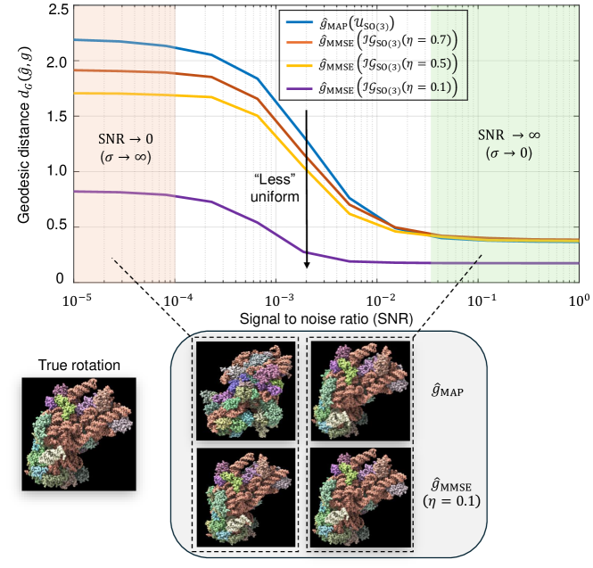
Figure 2: Impact of incorporating the prior rotational distribution on estimation accuracy. In all cases, the true underlying rotational distribution is modeled as an isotropic Gaussian distribution $\mathcal{IG}_{\mathsf{SO}(3)}(\eta=0.1)$. The metric used for comparison is the geodesic distance, as defined in (2.5). Here, $g$ denotes the true rotation, $\hat{g}_{\mathrm{MAP}}$ represents the MAP estimator from (3.3), and $\hat{g}_{\mathrm{MMSE}}$ denotes the Bayesian MMSE estimator from (3.2). The MMSE estimators are evaluated using different isotropic Gaussian distributions over the rotation group $\mathsf{SO}(3)$ with varying variances $\eta=0.7,0.5$, and $0.1$, respectively (see Appendix B). As the variance parameter $\eta$ decreases, resulting in less uniform rotational distribution closer to the true underlying rotational distribution, the accuracy of the MMSE rotation estimation improves. Each point in the curve plot is based on Monte Carlo simulations with 10,000 trials, using a sampling grid size of $L=300$. Below the curve plot, an illustration of colored 3D volumes, generating according to different rotational estimators, compares the performance of the MAP and MMSE estimators, where the second row on the right corresponds to using the true prior distribution $\mathcal{IG}_{\mathsf{SO}(3)}(\eta=0.1)$ in the MMSE estimation process. Clearly, the MMSE estimator leads to a more accurate rotation estimation.

The impact of sampling grid size $L$ and SNR on estimation accuracy.

To study these effects, we restrict ourselves to the uniform rotational distribution setting. Figure 3 illustrates the impact of the sampling grid size of $\mathsf{SO}(3)$ together with different levels of SNR, on the geodesic distance between the MAP and MMSE rotation estimators relative to the true rotations. Several observations can be made. First, at high SNR levels, the MAP and MMSE estimators nearly coincide, as predicted by Proposition 2.1. In this regime, the geodesic distance scales empirically as $L^{1/3}$. This relationship can be attributed to the representation of the $\mathsf{SO}(3)$ rotation using three parameters, which leads to a typical grid size that scales as $L^{1/3}$ in each direction. As the SNR decreases, the disparity between the different estimators diminishes as a function of the grid sampling size $L$. Additionally, in the extreme case where $\sigma\to\infty$, the mean geodesic distance appears to be similar for both the MAP and MMSE estimators, showing no dependence on the grid size $L$.

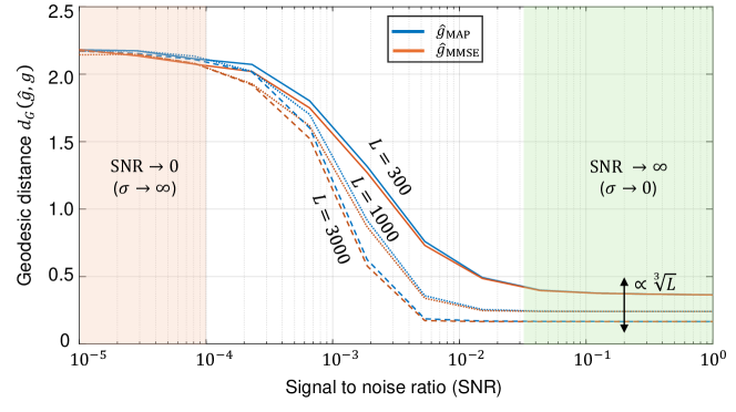
Figure 3: Impact of the sampling grid size of $\mathsf{SO}(3)$ ($L$) and the signal-to-noise ratio (SNR) on rotation estimation accuracy. This figure shows the accuracy of rotation estimation under varying sampling grid sizes $L$ of the rotation group $\mathsf{SO}(3)$ and different SNR levels of the observed data $y$ in the model (2.1). The metric used for comparison is the geodesic distance, as defined in (2.5). Here, $g$ denotes the true rotation, $\hat{g}_{\mathrm{MAP}}$ represents the MAP estimator from (3.3), and $\hat{g}_{\mathrm{MMSE}}$ denotes the Bayesian MMSE estimator from (3.2). In the high SNR regime ($\sigma\to 0$), the MAP and MMSE estimators converge, and the geodesic distance scales empirically as $\propto L^{1/3}$. This scaling reflects the three-parameter nature of $\mathsf{SO}(3)$ rotations, where the resolution of the sampling grid improves as $L$ increases. The results shown are based on Monte Carlo simulations with 3000 trials per data point.

4 Bayesian rotation determination as part of the volume reconstruction problem

Thus far, we have introduced the MAP and MMSE rotation estimators for estimating the rotation between a single noisy observation $y$ and a reference volume $\overline{V}$, as defined in (2.1). An intriguing question that arises is how these estimators can be utilized and influence performance within a 3D volume reconstruction process, which constitutes the main computational challenge in cryo-EM and cryo-ET.

Structure reconstruction typically follows two primary approaches: hard-assignment or soft-assignment methods, which are generally implemented through iterative refinement. In the hard-assignment approach, each observation is assigned a single orientation based on the highest correlation, and the 3D structure is then reconstructed given the rotations. In contrast, the soft-assignment method assigns probabilities across all possible orientations for each observation, enabling the 3D structure to be recovered as a weighted average of the observations, with weights determined by these probabilities. The iterative application of the soft-assignment procedure aligns with the EM algorithm [12, 46], which serves as the core computational method in modern cryo-EM [44, 40].

In the following, we demonstrate that incorporating the MMSE rotation estimator into the volume reconstruction process in the cryo-ET model (without projections) resembles the expectation-maximization (EM) algorithm, as it accounts for the full distribution of possible outcomes. In contrast, substituting the MAP estimator into the algorithm operates more like a hard-assignment reconstruction method, focusing exclusively on the most likely outcome. This distinction underscores the broader applicability and flexibility of the Bayes estimator in capturing uncertainty and delivering more accurate estimates for structure reconstruction.

4.1 Connection to the EM algorithm in volume reconstruction without projection

Unlike the previous orientation estimation model (2.1), we consider the following simplified model for volume reconstruction (see also [48, 4, 14]). We observe $M$ i.i.d samples taking the form

$$y_{i}=g_{i}^{-1}\cdot V+\varepsilon_{i},\quad\quad i=1,\ldots,M,$$ (4.1)

where $V$ is 3D volume structure of interest, $\{g_{i}\}_{i=0}^{M-1}\in\mathsf{SO}(3)$ are unknown latent variables following i.i.d. uniform distribution and $\{\varepsilon_{i}\}_{i=0}^{M-1}$ are i.i.d isotropic Gaussian noise with variance $\sigma^{2}$. The goal is to recover $V$ from the observations $\{y_{i}\}_{i=0}^{M-1}$, treating the rotations $\{g_{i}\}_{i=0}^{M-1}$ as latent variables.

To distinguish the model (4.1) from (2.1), we highlight the key differences as follows:

• The parameter of interest is the unknown structure $V$ here, whereas it was the single rotation $g$ in model (2.1);

• We observe $M$ i.i.d. samples instead of a single observation, meaning that all observed $M$ samples are used collectively to estimate the underlying volume structure $V$;

• Although the rotations $\{g_{i}\}_{i=0}^{M-1}$ are also unknown, they are treated as nuisance parameters, and we are not directly concerned with their estimation (though admittedly, more accurate estimation of $\{g_{i}\}_{i=0}^{M-1}$ could often contribute to better estimation of $V$).

For the case where $V$ represents a 2D image, $\{g_{i}\}_{i=0}^{M-1}\in\mathsf{SO}(2)$ corresponds to in-plane rotations, and the model is used for image recovery (see more in Section 4.2) [31].

The most common approach to solve this reconstruction problem is through the EM algorithm that applies soft-assignment iteratively as detailed in Algorithm 2. At each new iteration, the algorithm utilizes the volume estimate from the previous iteration, denoted as $\hat{V}^{(t)}$, to update the estimation of the volume $\hat{V}^{(t+1)}$, based on the observations $\left\{y_{i}\right\}_{i=0}^{M-1}$. The following proposition shows the relation between the update rule of the volume structure estimation at iteration $t+1$, and the MMSE rotation-determination estimator as introduced (2.11).

Algorithm 2 EM algorithm for volume reconstruction

Input: An initial volume $\hat{V}^{(0)}$, number of iteration $T$ and observations $\left\{y_{i}\right\}_{i=0}^{M-1}$ given by (4.1).
Output: Final volume estimation after $T$ iteration, $\hat{V}^{(T)}$.
Each Iteration, for $t=0\ldots,T-1$:

1. Compute for every $0\leq i\leq M-1$:

   $$p_{i}^{(t)}(g)=\frac{\exp\Big{(}-\left\|y_{i}-\left(g^{-1}\cdot\hat{V}^{(t)}\right)\right\|^{2}/2\sigma^{2}\Big{)}}{\int_{g\in\mathsf{SO}(3)}\exp\Big{(}-\left\|y_{i}-\left(g^{-1}\cdot\hat{V}^{(t)}\right)\right\|^{2}/2\sigma^{2}\Big{)}\mathrm{d}g},$$ (4.2)

2. Update the volume estimate:

   $$\hat{V}^{(t+1)}= \underset{V}{\operatorname*{arg\,min}}\sum_{i=0}^{M-1}\int_{g\in\mathsf{SO}(3)}p_{i}^{(t)}(g)\left\|y_{i}-\left(g^{-1}\cdot V\right)\right\|^{2}\mathrm{d}g$$

   $$= \sum_{i=0}^{M-1}\int_{g\in\mathsf{SO}(3)}p_{i}^{(t)}(g)(g\cdot y_{i})\mathrm{d}g.$$ (4.3)

Proposition 4.1.

Let $\hat{V}^{(t+1)}$ be the $(t+1)$-th volume estimator in the EM algorithm as described in Algorithm 2. Then, the M-step update has the form

$$\hat{V}^{(t+1)}=\frac{1}{M}\sum_{i=0}^{M-1}\hat{g}_{\mathsf{MMSE},i,t}\cdot y_{i},$$ (4.4)

where $\hat{g}_{\mathsf{MMSE},i,t}$ is the rotation MMSE estimator with respect to the uniform prior given observation $y_{i}$ and underlying structure $\hat{V}^{(t)}$ as introduced in (2.11)

$$\hat{g}_{\mathsf{MMSE},i,t}=\mathbb{E}[g|y_{i},\hat{V}^{(t)}]=\int_{g\in\mathsf{SO}(3)}\ p_{i}^{(t)}(g)g\mathrm{d}g,$$ (4.5)

with $\mathrm{d}g$ corresponds to the uniform distribution over $\mathsf{SO}(3)$.

The proof of this proposition is presented in Appendix C. In words, the proposition shows that the update rule for the volume structure estimation at iteration $t+1$, given the volume $\hat{V}^{(t)}$, is equivalent to aligning each observation $\left\{y_{i}\right\}_{i=0}^{M-1}$ using the associated MMSE estimator $\hat{g}_{\text{MMSE},i,t}$, computed based on the reference volume $\hat{V}^{(t)}$, and then averaging the aligned observations (4.4). Thus, the MMSE rotation-determination estimator is a key ingredient in the EM algorithm for volume reconstruction.

The MAP estimator as part of volume reconstruction.

In contrast to the soft assignment procedure, if we replace the MMSE estimator with the MAP estimator $\hat{g}_{\text{MAP}}$, we obtain the structure reconstruction algorithm by applying hard assignment iteratively. To be more specific, the MAP estimator applied to the observations $\left\{y_{i}\right\}_{i=0}^{M-1}$ can be viewed as a hard assignment among all possible rotations. In practice, this procedure involves making a hard decision where a single rotation is selected from the rotation grid according to the closest alignment. In the $(t+1)$-th iteration, similarly to (4.4), the hard-assignment process can be expressed as follows:

$$\hat{V}^{(t+1)}=\frac{1}{M}\sum_{i=0}^{M-1}\hat{g}_{\mathsf{MAP},i,t}\cdot y_{i},$$ (4.6)

where $\hat{g}_{\mathsf{MAP},i,t}$ is defined by

$$\hat{g}_{\mathsf{MAP},i,t}= \operatorname*{arg\,max}_{g\in\mathsf{SO}(3)}{\mathbb{P}}(g|y_{i},\hat{V}^{(t)})=\operatorname*{arg\,min}_{g\in\mathsf{SO}(3)}\|y_{i}-(g^{-1}\cdot\hat{V}^{(t)})\|^{2}.$$ (4.7)

4.2 Empirical results for volume reconstruction and the “Einstein from Noise” phenomenon

We demonstrate empirically volume reconstruction by applying the MAP estimator $\hat{g}_{\mathsf{MAP}}$ and the MMSE estimator $\hat{g}_{\mathsf{MMSE}}$ as part of the reconstruction problem, as specified in (4.6) and (4.4), respectively.

Description of the experiments.

We demonstrate the reconstruction process, which integrates MAP and MMSE rotation estimation as intermediate steps, using the two examples: 2D image recovery (Figure 4) and 3D volume reconstruction without projection (Figure 5). The iterative reconstruction process, as outlined in Algorithm 2, was performed until convergence (i.e., when the relative difference between consecutive iterations fell below a predefined threshold) or until reaching a maximum of 100 iterations.

Figures 4 and 5 were generated using slightly different methods. For the 2D experiment presented in Figure 4, we used polar coordinates, while in the 3D experiment, shown in Figure 5, we used a standard Cartesian basis. The primary difference lies in the interpolation required for producing Figure 5, which utilizes cubic interpolation for each observation based on the estimated rotation. This introduces certain “quantization” errors. Additionally, as detailed in Section 2, the 3D reconstruction process, presented in Figure 5, requires a “rounding” step which amounts to solving the Orthogonal Procrustes procedure.

In Figure 4, the true and template structures were generated in a polar representation with $d=300$ radial points and $L=30$ polar angle points. The reconstruction process was performed with $M=5\times 10^{4}$ observations. The additive noise was added in the polar representation. In Figure 5, $M=3000$ observations were used, with the rotation group $\mathsf{SO}(3)$ grid size of $L=300$.

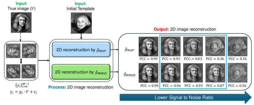
Figure 4: Comparison of 2D image recovery using the MMSE and the MAP rotation estimators. Iterative image recovery procedures with the MMSE estimator ($\hat{g}_{\text{MMSE}}$) and MAP estimator ($\hat{g}_{\text{MAP}}$) are defined in (4.4) and (4.6), respectively. The experiment employs a template image of Einstein and a ground truth image of Newton, both rotated in 2D over a uniform polar grid with $L=30$ samples. The reconstructed images within the light-blue rectangle (right panel) show superior performance with the MMSE rotation estimator, with Pearson cross-correlation (PCC) provided for each reconstructed image. The MAP and MMSE reconstructions are nearly identical at high SNR ($\sigma\to 0$), as predicted by Proposition 2.1. At very low SNR ($\sigma\to\infty$), the “Einstein from Noise” effect appears, where the estimator resembles the template image of Einstein rather than the underlying truth of Newton. In intermediate SNR ranges, using the MMSE estimator in the iterative step clearly outperforms the MAP estimator.

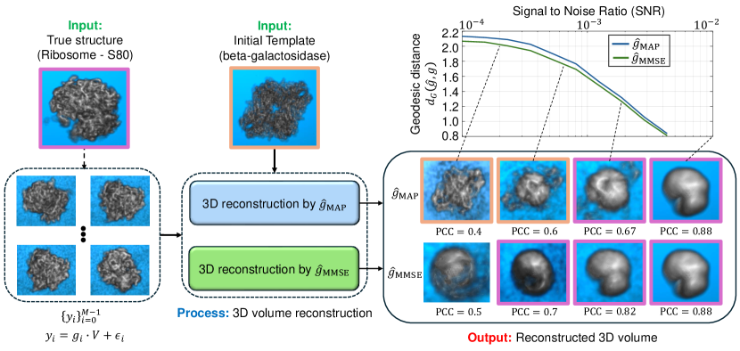
Figure 5: Comparison of 3D structure reconstruction in cryo-ET subtomograms averaging using the MMSE and MAP rotation estimators. Iterative structure reconstruction procedures with the MMSE estimator ($\hat{g}_{\text{MMSE}}$) and MAP estimator ($\hat{g}_{\text{MAP}}$) are defined in (4.4) and (4.6), respectively. At high SNR levels, a low-resolution structure emerges due to finite grid sampling of the rotation group $\mathsf{SO}(3)$, effectively acting as a low-pass filter. The 3D reconstruction using the MMSE estimator consistently outperforms the reconstruction using the MAP estimator. For high SNR conditions (i.e., $\sigma\to 0$), both estimators yield similar 3D structures, as expected from Proposition 2.1. The SNR values used for the panels (from right to left) are $10^{-2}$, $2\times 10^{-3}$, $7\times 10^{-4}$, and $2\times 10^{-4}$. The boxes highlighted in purple resemble the true input structure (Ribosome-S80 [59]), while the orange-highlighted boxes are more similar to the initial template (beta-galactosidase [6]), illustrating the “Einstein from Noise” phenomenon. Notably, at very low SNRs, the “Einstein from Noise” effect is evident with the MAP estimator but not with the MMSE estimator. In the “Einstein from Noise” regime, high-frequency details remain unfiltered, revealing finer structural features, in contrast to the suppressed high-frequency information in the accurate 3D reconstruction.

Empirical observations.

A few observations can be made from both Figures 4 and 5. First, in the case of high SNR (i.e., as $\sigma\to 0$), the volume reconstruction is similar whether using the MAP estimator or the MMSE estimator. This similarity is theoretically inferred by Proposition 2.1. However, as the SNR decreases, the reconstructions diverge, with the volumes reconstructed using the MMSE estimator showing a better correlation with the true volume. Second, in scenarios of extremely low SNR, where the structural signal is nearly nonexistent, the phenomenon known as “Einstein from Noise” manifests in both 2D and 3D contexts. This phenomenon pertains to the inherent model bias within the reconstruction procedure, specifically in relation to the initial templates. In such cases, the reconstructed volume exhibits structural similarities to the initial template, even though the observations do not substantiate this outcome. The generation of a structured image from entirely noisy data has attracted considerable attention, particularly during a significant scientific debate regarding the structure of an HIV molecule [34, 19, 57, 52, 33]; for a comprehensive description and statistical analysis, see [3, 2]. Notably, our empirical evidence suggests that the “Einstien from Noise” phenomenon is more pronounced when adopting the MAP estimator compared to the MMSE estimator, implying that the MMSE approach is less vulnerable to the choice of the initial template. Furthermore, our experiment implies the advantage of using the Bayesian MMSE estimator over the MAP estimator is more significant in 3D structure reconstruction tasks compared to 2D image recovery, where the 3D setting is a problem of greater interest to researchers in structural biology.

5 Discussion and conclusions

In this work, we have introduced the Bayesian framework for enhancing orientation estimation for various applications in structural biology. The proposed approach offers greater flexibility and improved accuracy compared to existing methods, with the MMSE estimator as a prime example. This technique handles diverse structural conformations and arbitrary rotational distributions across sample sets. Our empirical results establish that the proposed MMSE estimator consistently surpasses the performance of the current methods, particularly in challenging low SNR environments, as well as when prior information on rotational distribution is available or approximately known. We provide a theoretical foundation to explain these performance gains. As rotation determination is crucial for both 2D and 3D reconstruction processes, we further illustrate how utilizing the MMSE estimator as a soft-assignment step in iterative refinement leads to significant improvements over hard-assignment methods. Moreover, the proposed Bayesian approach empirically offers enhanced resilience against the “Einstein from Noise” phenomenon, effectively reducing model bias and improving the overall reliability of structural reconstructions. Thus, our main recommendation is to adopt the Bayesian MMSE rotation estimator over the MAP estimator in related application scenarios. Already integrated into most software, the Bayesian rotation estimator can be easily implemented with minimal computational cost, offering improved accuracy and resilience for orientation determination and structure reconstruction.

Future work.

This study has primarily focused on the Bayes estimator with respect to the MSE loss function; however, exploring alternative loss functions beyond MSE presents an exciting avenue for future research. While the Bayes estimator with MSE has a closed-form solution, other loss functions typically lack analytic solutions, necessitating numerical estimation methods. Investigating the impact of different loss functions on 3D reconstruction accuracy would provide valuable insights. For instance, recent studies have demonstrated the effectiveness of the Wasserstein distance as a loss function for rotation estimation [50].

Another promising direction is the direct estimation of the rotational distribution from observations and integrating this information into the rotation estimation process or EM algorithms for 3D structure reconstruction [23]. Such an approach could significantly improve rotation estimation accuracy, particularly in low SNR regimes, as suggested by the results in Figure 2, and could potentially enhance volume reconstruction. Additional extensions could include modeling greater structural uncertainties, which is common in scenarios involving flexible proteins, and addressing general pose determination problems that encompass rotations and translations. Finally, leveraging the Bayesian framework to derive confidence regions for individual rotations offers another interesting research direction, potentially enhancing interpretability and reliability in rotation estimation tasks.

Data Availability

The data underlying the results presented in this paper are not publicly available at this time but may be obtained from the authors upon request.

Appendix

Appendix A Proof of Proposition 2.1

By the definition in (2.11), assuming a uniform distribution of $\Lambda$ over $\mathsf{SO}(3)$ and that $\tilde{\Sigma}=\sigma^{2}I_{d\times d}$, we have:

$$\hat{g}_{\mathsf{MMSE}}= \mathbb{E}[g|y,\overline{V}]$$

$$= \frac{\int_{\mathsf{SO}(3)}g\exp\Big{(}-\frac{1}{2}(y-\Pi(g^{-1}\cdot\overline{V}))^{\mathsf{T}}\tilde{\Sigma}^{-1}(y-\Pi(g^{-1}\cdot\overline{V}))\Big{)}\mathrm{d}g}{\int_{\mathsf{SO}(3)}\exp\Big{(}-\frac{1}{2}(y-\Pi(g^{-1}\cdot\overline{V}))^{\mathsf{T}}\tilde{\Sigma}^{-1}(y-\Pi(g^{-1}\cdot\overline{V}))\Big{)}\mathrm{d}g}$$

$$=\frac{\int_{\mathsf{SO}(3)}g\exp\Big{(}-\left\|y-\Pi(g^{-1}\cdot\overline{V})\right\|^{2}/2\sigma^{2}\Big{)}\mathrm{d}g}{\int_{\mathsf{SO}(3)}\exp\Big{(}-\left\|y-\Pi(g^{-1}\cdot\overline{V})\right\|^{2}/2\sigma^{2}\Big{)}\mathrm{d}g}.$$ (A.1)

To prove the proposition, we apply the following known theorem [41, Theorem 5.10]:

Theorem A.1.

Consider $h$ a real-values function defined on a closed and bounded set, $\Theta$, of $\mathbb{R}^{p}$. If there exists a unique solution $\theta^{*}$ satisfying

$$\theta^{*}=\underset{\theta\in\Theta}{\operatorname*{arg\,max}}\ h(\theta),$$ (A.2)

then

$$\underset{\lambda\to\infty}{\lim}\frac{\int_{\Theta}\theta e^{\lambda h(\theta)}d\theta}{\int_{\Theta}e^{\lambda h(\theta)}d\theta}=\theta^{*}.$$ (A.3)

Let us define the function $h(g)$ as follows:

$$h(g)\triangleq-\left\|y-\Pi(g^{-1}\cdot\overline{V})\right\|^{2}.$$ (A.4)

Under the assumption of the proposition that $\hat{g}_{\mathsf{MAP}}$ is unique, and given the definition of $\hat{g}_{\mathsf{MAP}}$ in (2.10), the function $h$ satisfies the conditions of Theorem A.1, and its unique maximizer is $\hat{g}_{\mathsf{MAP}}$, i.e.,

$$\hat{g}_{\mathsf{MAP}}=\underset{g\in\mathsf{SO}(3)}{\operatorname*{arg\,max}}\ h(g).$$ (A.5)

Then, applying Theorem A.1 for $\lambda=1/2\sigma^{2}$ and using (A.5), we obtain:

$$\lim_{\sigma\to 0}\hat{g}_{\mathrm{MMSE}} =\lim_{\sigma\to 0}\frac{\int_{\mathsf{SO}(3)}g\exp\Big{(}-\left\|y-\Pi(g^{-1}\cdot\overline{V})\right\|^{2}/2\sigma^{2}\Big{)}\mathrm{d}g}{\int_{\mathsf{SO}(3)}\exp\Big{(}-\left\|y-\Pi(g^{-1}\cdot\overline{V})\right\|^{2}/2\sigma^{2}\Big{)}\mathrm{d}g}$$

$$=\lim_{\lambda\to\infty}\frac{\int_{\mathsf{SO}(3)}g\exp\Big{(}-\lambda\left\|y-\Pi(g^{-1}\cdot\overline{V})\right\|^{2}\Big{)}\mathrm{d}g}{\int_{\mathsf{SO}(3)}\exp\Big{(}-\lambda\left\|y-\Pi(g^{-1}\cdot\overline{V})\right\|^{2}\Big{)}\mathrm{d}g}$$

$$=\underset{g\in\mathsf{SO}(3)}{\operatorname*{arg\,max}}\ h(g)=\hat{g}_{\mathsf{MAP}},$$ (A.6)

which proves the proposition.

Appendix B Isotropic Gaussian distribution of SO(3) rotations

The IG distribution $\mathcal{I}\mathcal{G}_{\mathsf{SO}(3)}(\eta)$, parameterized by the scalar variance $\eta^{2}$, can be represented in an axis-angle form, with uniformly sampled axes and a rotation angle $\omega\in[0,\pi]$, having the following probability density function [42]:

$$f(\omega)=\frac{1-\cos\omega}{\pi}\sum_{\ell=0}^{\infty}(2\ell+1)e^{-\ell(\ell+1)\eta^{2}}\frac{\sin\left((\ell+1/2)\omega\right)}{\sin(\omega/2)}.$$ (B.1)

Notably, the uniform distribution on $\mathsf{SO}(3)$, denoted $\mathcal{U}_{\mathsf{SO}(3)}$, corresponds to uniformly sampled axes and is characterized by the density function $f(\omega)=\frac{1-\cos\omega}{\pi}$, which represents the limiting case of $\eta\to\infty$ in (B.1).

For $\eta>1$, the series converges quickly, and $\ell_{\text{max}}=5$ is typically sufficient for sub-percent accuracy. However, as $\eta$ decreases, convergence becomes slower, making it inefficient for modeling concentrated distributions. Fortunately, this series has been well studied, and an excellent approximation for $\eta<1$ has been proposed in the literature [35], given by the following closed-form approximation:

$$f(\omega)\simeq\frac{1-\cos\omega}{\sqrt{\pi}}\eta^{-\frac{3}{2}}e^{\left(\frac{\eta}{4}-\frac{\left(\omega/2\right)^{2}}{\eta}\right)}\left(\frac{\omega-e^{-\pi^{2}/\eta}\left(\left(\omega-2\pi\right)e^{\pi\omega/\eta}+\left(\omega+2\pi\right)e^{-\pi\omega/\eta}\right)}{2\sin\left(\frac{\omega}{2}\right)}\right).$$ (B.2)

The method for generating samples according to the isotropic Gaussian distribution on $\mathsf{SO}(3)$ relies on the inverse sampling theorem. This technique enables sampling from a specified probability distribution by utilizing its cumulative distribution function (CDF). Specifically, it involves generating a uniform random number between 0 and 1 and then applying the inverse CDF to obtain a sample from the target distribution [42].

Appendix C Proof of Proposition 4.1

Following (4.3), the update law (M-step) of the $t+1$ iteration of the expectation-maximization algorithm is given by:

$$\hat{V}^{(t+1)}=\underset{V}{\operatorname*{arg\,min}}\sum_{i=0}^{M-1}\int_{g\in\mathsf{SO}(3)}p_{i}^{(t)}(g)\left\|y_{i}-\left(g^{-1}\cdot V\right)\right\|^{2}\mathrm{d}g,$$ (C.1)

where

$$p_{i}^{(t)}(g)=\frac{\exp\Big{(}-\left\|y_{i}-\left(g^{-1}\cdot\hat{V}^{(t)}\right)\right\|^{2}/2\sigma^{2}\Big{)}}{\int_{g\in\mathsf{SO}(3)}\exp\Big{(}-\left\|y_{i}-\left(g^{-1}\cdot\hat{V}^{(t)}\right)\right\|^{2}/2\sigma^{2}\Big{)}\mathrm{d}g}.$$ (C.2)

As the action by the group element $g$ preserves the norm, we have,

$$\left\|y_{i}-\left(g^{-1}\cdot V\right)\right\|^{2}=\left\|g\cdot{y_{i}}-V\right\|^{2}=\left\|g\cdot y_{i}\right\|^{2}+\left\|V\right\|^{2}-2{\,\langle{g\cdot y_{i}},V\rangle}.$$ (C.3)

Thus, substituting (C.3) into (C.1), leads to:

$$\hat{V}^{(t+1)}=\underset{V}{\operatorname*{arg\,min}}\sum_{i=0}^{M-1}\int_{g\in\mathsf{SO}(3)}p_{i}^{(t)}(g)\left\{\left\|g\cdot y_{i}\right\|^{2}+\left\|V\right\|^{2}-2{\,\langle{g\cdot y_{i}},V\rangle}\right\}\mathrm{d}g.$$ (C.4)

As the term $\left\|g\cdot y_{i}\right\|^{2}$ is independent of $V$, (C.4) can be simplified to:

$$\hat{V}^{(t+1)}=\underset{V}{\operatorname*{arg\,min}}\sum_{i=0}^{M-1}\int_{g\in\mathsf{SO}(3)}p_{i}^{(t)}(g)\left\{\left\|V\right\|^{2}-2{\,\langle{g\cdot y_{i}},V\rangle}\right\}\mathrm{d}g.$$ (C.5)

Let us denote by $h(V)$ the right hand side of (C.5):

$$h(V)\triangleq\sum_{i=0}^{M-1}\int_{g\in\mathsf{SO}(3)}p_{i}^{(t)}(g)\left\{\left\|V\right\|^{2}-2{\,\langle{g\cdot y_{i}},V\rangle}\right\}\mathrm{d}g.$$ (C.6)

Taking the first-order condition with respect to $V$ gives

$$\frac{\partial}{\partial V}h(V)=2\sum_{i=0}^{M-1}\int_{g\in\mathsf{SO}(3)}p_{i}^{(t)}(g)\left(V-g\cdot y_{i}\right)\mathrm{d}g=0.$$ (C.7)

As $\int_{g\in\mathsf{SO}(3)}p_{i}^{(t)}(g)=1$ for every $i$, we can simplify (C.7) to obtain:

$$V=\frac{1}{M}\sum_{i=0}^{M-1}\int_{g\in\mathsf{SO}(3)}gp_{i}^{(t)}(g)\mathrm{d}g.$$ (C.8)

The integral in the right-hand-side of (C.8) is nothing but $\hat{g}_{\mathsf{MMSE},i,t}$ as defined in (4.5). Thus, we obtain

$$\hat{V}^{(t+1)}=\frac{1}{M}\sum_{i=0}^{M-1}\hat{g}_{\mathsf{MMSE},i,t}\cdot y_{i},$$ (C.9)

which proves the proposition.

References

- [1] Xiao-Chen Bai, Greg McMullan, and Sjors HW Scheres. How cryo-EM is revolutionizing structural biology. Trends in biochemical sciences, 40(1):49–57, 2015.
- [2] Amnon Balanov, Tamir Bendory, and Wasim Huleihel. Confirmation bias in Gaussian mixture models. arXiv preprint arXiv:2408.09718, 2024.
- [3] Amnon Balanov, Wasim Huleihel, and Tamir Bendory. Einstein from noise: Statistical analysis. arXiv preprint arXiv:2407.05277, 2024.
- [4] Afonso S Bandeira, Ben Blum-Smith, Joe Kileel, Jonathan Niles-Weed, Amelia Perry, and Alexander S Wein. Estimation under group actions: recovering orbits from invariants. Applied and Computational Harmonic Analysis, 66:236–319, 2023.
- [5] Afonso S Bandeira, Yutong Chen, Roy R Lederman, and Amit Singer. Non-unique games over compact groups and orientation estimation in cryo-EM. Inverse Problems, 36(6):064002, 2020.
- [6] Alberto Bartesaghi, Doreen Matthies, Soojay Banerjee, Alan Merk, and Sriram Subramaniam. Structure of -galactosidase at 3.2-å resolution obtained by cryo-electron microscopy. Proceedings of the National Academy of Sciences, 111(32):11709–11714, 2014.
- [7] Tamir Bendory, Alberto Bartesaghi, and Amit Singer. Single-particle cryo-electron microscopy: Mathematical theory, computational challenges, and opportunities. IEEE signal processing magazine, 37(2):58–76, 2020.
- [8] Tamir Bendory, Nicolas Boumal, William Leeb, Eitan Levin, and Amit Singer. Toward single particle reconstruction without particle picking: Breaking the detection limit. SIAM Journal on Imaging Sciences, 16(2):886–910, 2023.
- [9] Tamir Bendory, Nicolas Boumal, Chao Ma, Zhizhen Zhao, and Amit Singer. Bispectrum inversion with application to multireference alignment. IEEE Transactions on signal processing, 66(4):1037–1050, 2017.
- [10] Gabriele Corso, Bowen Jing, Regina Barzilay, Tommi Jaakkola, et al. Diffdock: Diffusion steps, twists, and turns for molecular docking. In International Conference on Learning Representations (ICLR 2023), 2023.
- [11] JM De la Rosa-Trevín, Joaquin Otón, R Marabini, Airen Zaldívar, Javier Vargas, JM Carazo, and COS Sorzano. Xmipp 3.0: an improved software suite for image processing in electron microscopy. Journal of structural biology, 184(2):321–328, 2013.
- [12] Arthur P Dempster, Nan M Laird, and Donald B Rubin. Maximum likelihood from incomplete data via the EM algorithm. Journal of the royal statistical society: series B (methodological), 39(1):1–22, 1977.
- [13] Claire Donnat, Axel Levy, Frederic Poitevin, Ellen D Zhong, and Nina Miolane. Deep generative modeling for volume reconstruction in cryo-electron microscopy. Journal of structural biology, 214(4):107920, 2022.
- [14] Zhou Fan, Roy R Lederman, Yi Sun, Tianhao Wang, and Sheng Xu. Maximum likelihood for high-noise group orbit estimation and single-particle cryo-EM. The Annals of Statistics, 52(1):52–77, 2024.
- [15] Marc Aurele Gilles and Amit Singer. A Bayesian framework for cryo-EM heterogeneity analysis using regularized covariance estimation. bioRxiv, 2023.
- [16] John C Gower and Garmt B Dijksterhuis. Procrustes problems, volume 30. OUP Oxford, 2004.
- [17] Yael Harpaz and Yoel Shkolnisky. Three-dimensional alignment of density maps in cryo-electron microscopy. Biological Imaging, 3:e8, 2023.
- [18] Richard Hartley, Jochen Trumpf, Yuchao Dai, and Hongdong Li. Rotation averaging. International journal of computer vision, 103:267–305, 2013.
- [19] Richard Henderson. Avoiding the pitfalls of single particle cryo-electron microscopy: Einstein from noise. Proceedings of the National Academy of Sciences, 110(45):18037–18041, 2013.
- [20] Wolfgang Hörmann, Josef Leydold, and Gerhard Derflinger. Automatic nonuniform random variate generation. Springer Science & Business Media, 2013.
- [21] Du Q Huynh. Metrics for 3D rotations: Comparison and analysis. Journal of Mathematical Imaging and Vision, 35:155–164, 2009.
- [22] Yesukhei Jagvaral, Francois Lanusse, and Rachel Mandelbaum. Unified framework for diffusion generative models in SO(3): applications in computer vision and astrophysics. In Proceedings of the AAAI Conference on Artificial Intelligence, volume 38, pages 12754–12762, 2024.
- [23] Noam Janco and Tamir Bendory. An accelerated expectation-maximization algorithm for multi-reference alignment. IEEE Transactions on Signal Processing, 70:3237–3248, 2022.
- [24] Noam Janco and Tamir Bendory. Unrolled algorithms for group synchronization. IEEE Open Journal of Signal Processing, 2023.
- [25] Joe Kileel, Nicholas F Marshall, Oscar Mickelin, and Amit Singer. Fast expansion into harmonics on the ball. arXiv preprint arXiv:2406.05922, 2024.
- [26] Adam Leach, Sebastian M Schmon, Matteo T Degiacomi, and Chris G Willcocks. Denoising diffusion probabilistic models on so (3) for rotational alignment. In ICLR 2022 Workshop on Geometrical and Topological Representation Learning.
- [27] Erich L Lehmann and George Casella. Theory of point estimation. Springer Science & Business Media, 2006.
- [28] Eitan Levin, Tamir Bendory, Nicolas Boumal, Joe Kileel, and Amit Singer. 3D ab initio modeling in cryo-EM by autocorrelation analysis. In 2018 IEEE 15th International Symposium on Biomedical Imaging (ISBI 2018), pages 1569–1573. IEEE, 2018.
- [29] Bufan Li, Dongjie Zhu, Huigang Shi, and Xinzheng Zhang. Effect of charge on protein preferred orientation at the air–water interface in cryo-electron microscopy. Journal of Structural Biology, 213(4):107783, 2021.
- [30] Dmitry Lyumkis. Challenges and opportunities in cryo-EM single-particle analysis. Journal of Biological Chemistry, 294(13):5181–5197, 2019.
- [31] Chao Ma, Tamir Bendory, Nicolas Boumal, Fred Sigworth, and Amit Singer. Heterogeneous multireference alignment for images with application to 2D classification in single particle reconstruction. IEEE Transactions on Image Processing, 29:1699–1710, 2019.
- [32] M-E Mäeots and Radoslav I Enchev. Structural dynamics: review of time-resolved cryo-EM. Acta Crystallographica Section D: Structural Biology, 78(8):927–935, 2022.
- [33] Youdong Mao, Luis R Castillo-Menendez, and Joseph G Sodroski. Reply to Subramaniam, van Heel, and Henderson: Validity of the cryo-electron microscopy structures of the HIV-1 envelope glycoprotein complex. Proceedings of the National Academy of Sciences, 110(45):E4178–E4182, 2013.
- [34] Youdong Mao, Liping Wang, Christopher Gu, Alon Herschhorn, Anik Désormeaux, Andrés Finzi, Shi-Hua Xiang, and Joseph G Sodroski. Molecular architecture of the uncleaved HIV-1 envelope glycoprotein trimer. Proceedings of the National Academy of Sciences, 110(30):12438–12443, 2013.
- [35] Siegfried Matthies, J Muller, and GW Vinel. On the normal distribution in the orientation space. Texture, Stress, and Microstructure, 10(1):77–96, 1988.
- [36] Nina Miolane, Frédéric Poitevin, Yee-Ting Li, and Susan Holmes. Estimation of orientation and camera parameters from cryo-electron microscopy images with variational autoencoders and generative adversarial networks. In Proceedings of the IEEE/CVF Conference on Computer Vision and Pattern Recognition Workshops, pages 970–971, 2020.
- [37] Kazuyoshi Murata and Matthias Wolf. Cryo-electron microscopy for structural analysis of dynamic biological macromolecules. Biochimica et Biophysica Acta (BBA)-General Subjects, 1862(2):324–334, 2018.
- [38] Youssef SG Nashed, Frédéric Poitevin, Harshit Gupta, Geoffrey Woollard, Michael Kagan, Chun Hong Yoon, and Daniel Ratner. Cryoposenet: End-to-end simultaneous learning of single-particle orientation and 3D map reconstruction from cryo-electron microscopy data. In Proceedings of the IEEE/CVF International Conference on Computer Vision, pages 4066–4076, 2021.
- [39] Amelia Perry, Alexander S Wein, Afonso S Bandeira, and Ankur Moitra. Message-passing algorithms for synchronization problems over compact groups. Communications on Pure and Applied Mathematics, 71(11):2275–2322, 2018.
- [40] Ali Punjani, John L Rubinstein, David J Fleet, and Marcus A Brubaker. cryoSPARC: algorithms for rapid unsupervised cryo-EM structure determination. Nature methods, 14(3):290–296, 2017.
- [41] CP Robert. Monte carlo statistical methods, 1999.
- [42] TI Savjolova. Preface to novye metody issledovanija tekstury polikristalliceskich materialov. Metallurgija, Moscow, 4(2):6–2, 1985.
- [43] Sjors HW Scheres. A Bayesian view on cryo-EM structure determination. Journal of molecular biology, 415(2):406–418, 2012.
- [44] Sjors HW Scheres. RELION: implementation of a Bayesian approach to cryo-EM structure determination. Journal of structural biology, 180(3):519–530, 2012.
- [45] Yoel Shkolnisky and Amit Singer. Viewing direction estimation in cryo-EM using synchronization. SIAM journal on imaging sciences, 5(3):1088–1110, 2012.
- [46] Fred J Sigworth, Peter C Doerschuk, Jose-Maria Carazo, and Sjors HW Scheres. An introduction to maximum-likelihood methods in cryo-EM. In Methods in enzymology, volume 482, pages 263–294. Elsevier, 2010.
- [47] Amit Singer. Angular synchronization by eigenvectors and semidefinite programming. Applied and computational harmonic analysis, 30(1):20–36, 2011.
- [48] Amit Singer. Mathematics for cryo-electron microscopy. In Proceedings of the International Congress of Mathematicians: Rio de Janeiro 2018, pages 3995–4014. World Scientific, 2018.
- [49] Amit Singer and Yoel Shkolnisky. Three-dimensional structure determination from common lines in cryo-em by eigenvectors and semidefinite programming. SIAM journal on imaging sciences, 4(2):543–572, 2011.
- [50] Amit Singer and Ruiyi Yang. Alignment of density maps in Wasserstein distance. Biological Imaging, 4:e5, 2024.
- [51] Carlos Oscar S Sorzano, A Jiménez, Javier Mota, José Luis Vilas, David Maluenda, Marta Martínez, Erney Ramírez-Aportela, Tomas Majtner, J Segura, Ruben Sánchez-García, et al. Survey of the analysis of continuous conformational variability of biological macromolecules by electron microscopy. Acta Crystallographica Section F: Structural Biology Communications, 75(1):19–32, 2019.
- [52] Sriram Subramaniam. Structure of trimeric HIV-1 envelope glycoproteins. Proceedings of the National Academy of Sciences, 110(45):E4172–E4174, 2013.
- [53] Yong Zi Tan, Philip R Baldwin, Joseph H Davis, James R Williamson, Clinton S Potter, Bridget Carragher, and Dmitry Lyumkis. Addressing preferred specimen orientation in single-particle cryo-EM through tilting. Nature methods, 14(8):793–796, 2017.
- [54] Guang Tang, Liwei Peng, Philip R Baldwin, Deepinder S Mann, Wen Jiang, Ian Rees, and Steven J Ludtke. Eman2: an extensible image processing suite for electron microscopy. Journal of structural biology, 157(1):38–46, 2007.
- [55] Bogdan Toader, Fred J Sigworth, and Roy R Lederman. Methods for cryo-EM single particle reconstruction of macromolecules having continuous heterogeneity. Journal of molecular biology, 435(9):168020, 2023.
- [56] Marin Van Heel. Angular reconstitution: a posteriori assignment of projection directions for 3D reconstruction. Ultramicroscopy, 21(2):111–123, 1987.
- [57] Marin van Heel. Finding trimeric HIV-1 envelope glycoproteins in random noise. Proceedings of the National Academy of Sciences, 110(45):E4175–E4177, 2013.
- [58] Abigail JI Watson and Alberto Bartesaghi. Advances in cryo-ET data processing: meeting the demands of visual proteomics. Current Opinion in Structural Biology, 87:102861, 2024.
- [59] Wilson Wong, Xiao-chen Bai, Alan Brown, Israel S Fernandez, Eric Hanssen, Melanie Condron, Yan Hong Tan, Jake Baum, and Sjors HW Scheres. Cryo-EM structure of the Plasmodium falciparum 80S ribosome bound to the anti-protozoan drug emetine. Elife, 3:e03080, 2014.
- [60] Lingbo Yu, Robert R Snapp, Teresa Ruiz, and Michael Radermacher. Projection-based volume alignment. Journal of structural biology, 182(2):93–105, 2013.
- [61] Peijun Zhang. Advances in cryo-electron tomography and subtomogram averaging and classification. Current opinion in structural biology, 58:249–258, 2019.
- [62] Zhizhen Zhao and Amit Singer. Rotationally invariant image representation for viewing direction classification in cryo-em. Journal of structural biology, 186(1):153–166, 2014.
- [63] Ellen D Zhong, Tristan Bepler, Bonnie Berger, and Joseph H Davis. CryoDRGN: reconstruction of heterogeneous cryo-EM structures using neural networks. Nature methods, 18(2):176–185, 2021.