Interaction of jamitons in second-order macroscopic traffic models

Abstract.

Jamitons are self-sustained traveling wave solutions that arise in certain second-order macroscopic models of vehicular traffic. A necessary condition for a jamiton to appear is that the local traffic density breaks the so-called sub-characteristic condition. This condition states that the characteristic velocity of the corresponding first-order Lighthill-Whitham-Richards (LWR) model formed with the same desired speed function is enclosed by the characteristic speeds of the corresponding second-order model. The phenomenon of collision of jamitons in second-order models of traffic flow is studied analytically and numerically for the particular case of the second-order Aw-Rascle-Zhang (ARZ) traffic model [A. Aw, M. Rascle, SIAM J. Appl. Math. 60 (2000) 916–938; H. M. Zhang, Transp. Res. B 36 (2002) 275–290]. A compatibility condition is first defined to select jamitons that can collide each other. The collision of jamitons produces a new jamiton with a velocity different from the initial ones. It is observed that the exit velocities smooth out the velocity of the test jamiton and the initial velocities of the jamitons that collide. Other properties such as the amplitude of the exit jamitons, lengths, and maximum density are also explored. In the cases of the amplitude and maximum exit density it turns out that over a wide range of sonic densities, the exit values exceed or equal the input values. On the other hand, the resulting jamiton has a greater length than the incoming ones. Finally, the behavior for various driver reaction times is explored. It is obtained that some properties do not depend on that time, such as the amplitude, exit velocity, or maximum density, while the exit length does depend on driver reaction time.

1. Introduction

1.1. Scope

Jamitons are self-sustained traveling wave solutions that arise in second-order models of vehicular traffic. Here we understand as a second-order trafffic model as pair of one-dimensional balance equations that represent the analogues of conservation of mass and linear momentum in continuum mechanics. The notion of “jamiton”, an apparent amalgamation of traffic “jam” and “soliton”, was coined by Flynn et al. in [2], and studied in the context of the fundamental diagram of traffic flow by Seibold et al. [3]. The term “jamiton” is, however, not yet universally used in the traffic modelling literature (cf., e.g., [4, 5]). One widely studied second-order model that describes the formation of jamitons is the inhomogeneous Aw-Rascle-Zhang (ARZ) model [6, 7] given by

$$\begin{split}\partial_{t}\rho+\rho_{t}\partial_{x}(\rho u)&=0,\\ \partial_{t}\bigl{(}u+h(\rho)\bigr{)}+u\partial_{x}\bigl{(}u+h(\rho)\bigr{)}&=\dfrac{U(\rho)-u}{\tau},\end{split}$$ (1.1)

where $t$ is time, $x$ is spatial position, $\rho=\rho(x,t)$ is the sought density of vehicles (assumed to take values between zero and some maximal density $\rho_{\max}$), $u=u(x,t)$ is the unknown velocity, $h=h(\rho)$ is a strictly increasing hesitation function, $U=U(\rho)$ is the desired speed that is assumed to be a given decreasing function, and $\tau>0$ is a relaxation time. It is the purpose of the present work to undertake a mathematical study of the collision of jamitons for (1.1), elucidating the behavior of a jamiton following its collision with another jamiton, studying its size and output velocity. To the knowledge of the authors and known works, this type of study has not been undertaken previously.

1.2. Related work

From a mathematical standpoint, traffic models have been studied from at least three different perspectives in recent years, each distinguished by its own particular approach, namely microscopic models, cellular automata models, and macroscopic models. These approaches do not operate independently but are consistent in both their formulations and the phenomena encompassed. For instance, the simplest Nagel-Schreckenberg cellular automaton model [8] turns out to be a particular case of the numerical discretization of the macroscopic Lighthill-Whitham-Richards (LWR) model [9, 10]. Similarly, the discrete cell transmission model by Hilliges and Weidlich [11] represents a monotone numerical scheme for the LWR model that can even be extended to the multiclass case [12, 13]. We mainly focus here on macroscopic traffic models that describe vehicular traffic by a two-phase continuum approach. Introductions to this class of models include [4, 5, 14]. Macroscopic or continuous models no longer follow the behavior of individual vehicles but rather focus on vehicle density and the velocity field (the velocity present at a particular time and location). They are also related to microscopic or cellular automaton models. For example, in [15], equivalences between continuous and microscopic models are established, while in [16], equivalences with cellular automata are discussed.

This type of models presents several advantages for the study of vehicular traffic. For instance, they are preferred in terms of safety and data privacy as they do not access individual vehicle data directly. They also offer good precision and estimation at a large scale for noisy or sparse data [17, 18]. Moreover, they can be extended to routes with multiple lanes or to control problems [19]. Summarizing, macroscopic models usually give rise to partial differential equations (PDEs) or systems of PDEs, and many features of traffic flow can be derived from their qualitative properties as well as by applying numerical methods, see monographs on hyperbolic conservation laws and their numerical treatment (cf., e.g., [20, 21, 22, 23, 24]).

The authors’ interest in collisions of traffic flow interactions that should have a potentially complicated structure is in part motivated by the so-called conjectured fractal exit velocity that appears in dispersive collisions. An important simplified model of these phenomena is the well-known $\phi^{4}$ equation

$$\partial_{tt}\phi-\partial_{xx}\phi-\phi+\phi^{3}=0,\quad\phi(x,t)\in\mathbb{R},\quad(x,t)\in\mathbb{R}^{2}.$$ (1.2)

whose solutions may exhibit these collisions. (Equation (1.2) is also known under various other names, such as “$u$-4 model” [25] or “cubic Klein-Gordon equation” [26].) Equation (1.2) admits a family of traveling wave solutions, called kinks, that are given by

$$\phi(x,t)=\phi_{\mathrm{K}}(x-vt)=\tanh\left(\dfrac{x-x_{0}-vt}{\sqrt{2(1-v^{2})}}\right),$$ (1.3)

where $v\in(-1,1)$ is the (fixed) input velocity. On the other hand, the antikink solution corresponds to the same wave but traveling in the opposite direction, $\phi_{\bar{\mathrm{K}}}(x,t)=-\phi_{\mathrm{K}}(x+vt)$. From numerical simulations, one observes that equation (1.2) presents a fractal behavior for the output velocities after the collision, based on the input velocities. The phenomenon of the output velocities in the $\phi^{4}$ equation has been extensively studied in the literature, see e.g. [27, 28, 29, 30, 31, 32], where the phenomenon known as the “multiple-bounce” resonance effect is described mathematically.

1.3. Outline of the paper

In this paper we study, from a numerical point of view, collisions of jamitons, seeking to represent real-life jam collisions. This work is organized as follows. First of all, in Section 2 we present the macroscopic traffic models to be explored. Their properties, conditions, and relation to the fundamental diagram are discussed. In Section 3, the mathematical construction of jamitons is presented, including their definition, derivation from the traffic model, and several properties that they exhibit, in particular stability and asymptotic stability. In Section 4 a numerical scheme for the simulation of a jamiton is outlined. The scheme is validated by comparison with theoretical jamitons and results observed in the literature will be replicated, such as the emergence of jamitons on a long, essentially infinite, route. Finally, in Section 5, the procedure for the simulation of the collision of jamitons is described. This includes the initial configuration, conditions that jamitons must meet to collide, and the selection of jamitons. The chosen jamitons are caused to collide, and possible properties arising from the collision will be studied. Section 6 presents conclusions and future work.

2. Macroscopic models

2.1. Preliminaries

Macroscopic models describe vehicular traffic as two continuous phases (vehicles and the void space). The spatio-temporal evolution of vehicle density is modeled through scalar conservation PDEs. The main variables are usually the density $\rho=\rho(x,t)$, which represents the number of vehicles per unit length and will always is assumed nonnegative, the velocity field $u=u(x,t)$ that represents the local car velocity at position $x$ at time $t$, and the vehicle flow rate $Q=\rho u$, which indicates the number of vehicles passing a fixed point per unit of time. (Some important modifications to the previous setting are formulated within kinetic models. We will not consider these formulations here, but for a detailed introduction and results, including the collision phenomenon, see [33, 34, 35].) With these variables it is possible to deduce the principle of conservation of mass in integral form,

$$\frac{\mathrm{d}}{\mathrm{d}t}\int_{a}^{b}\rho(x,t)\,\mathrm{d}x=\rho(a,t)u(a,t)-\rho(b,t)u(b,t)\quad\text{for any interval $[a,b]\subset\mathbb{R}$ and $t\geq 0$,}$$ (2.1)

which indicates that vehicles are neither created nor destroyed, and from (2.1) we deduce the conservation PDE in differential form

$$\partial_{t}\rho+\partial_{x}(\rho u)=0.$$ (2.2)

The model (2.2) is still incomplete since there are two unknowns ($\rho$ and $u$) and only one equation. The well-known Lighthill-Whitham-Richards (LWR) model [9, 10] provides the required model closure via the kinematic assumption $u=u(\rho)$. In contrast, second-order models such as the ARZ model (1.1) or the Payne-Whitham (PW) model [36, 37] (to be outlined in Section 2.4) add a second equation for the velocity field that makes both variables $\rho$ and $u$ independent. Before continuing, it is necessary to introduce the concept of fundamental diagram for both first- and second-order traffic models. The fundamental diagram condenses the main properties to be encapsulated in macroscopic models, such as vehicular congestion or free flow at low densities.

2.2. Fundamental diagram

(a)	(b)

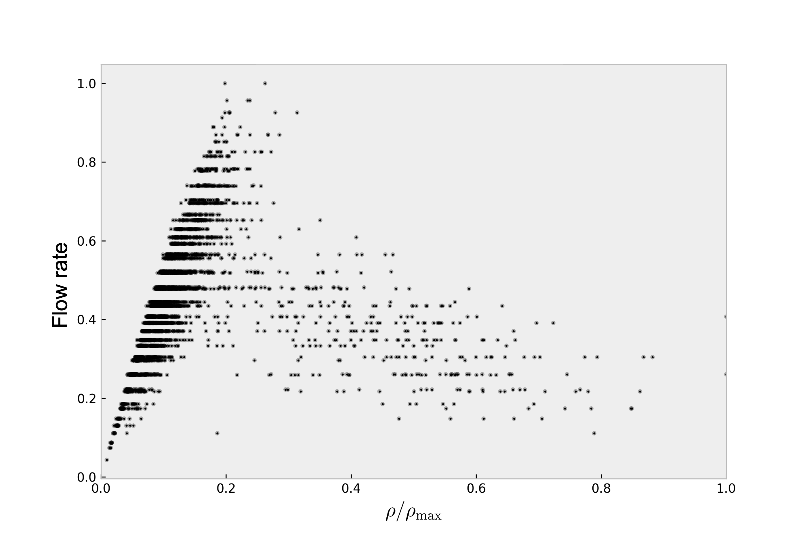
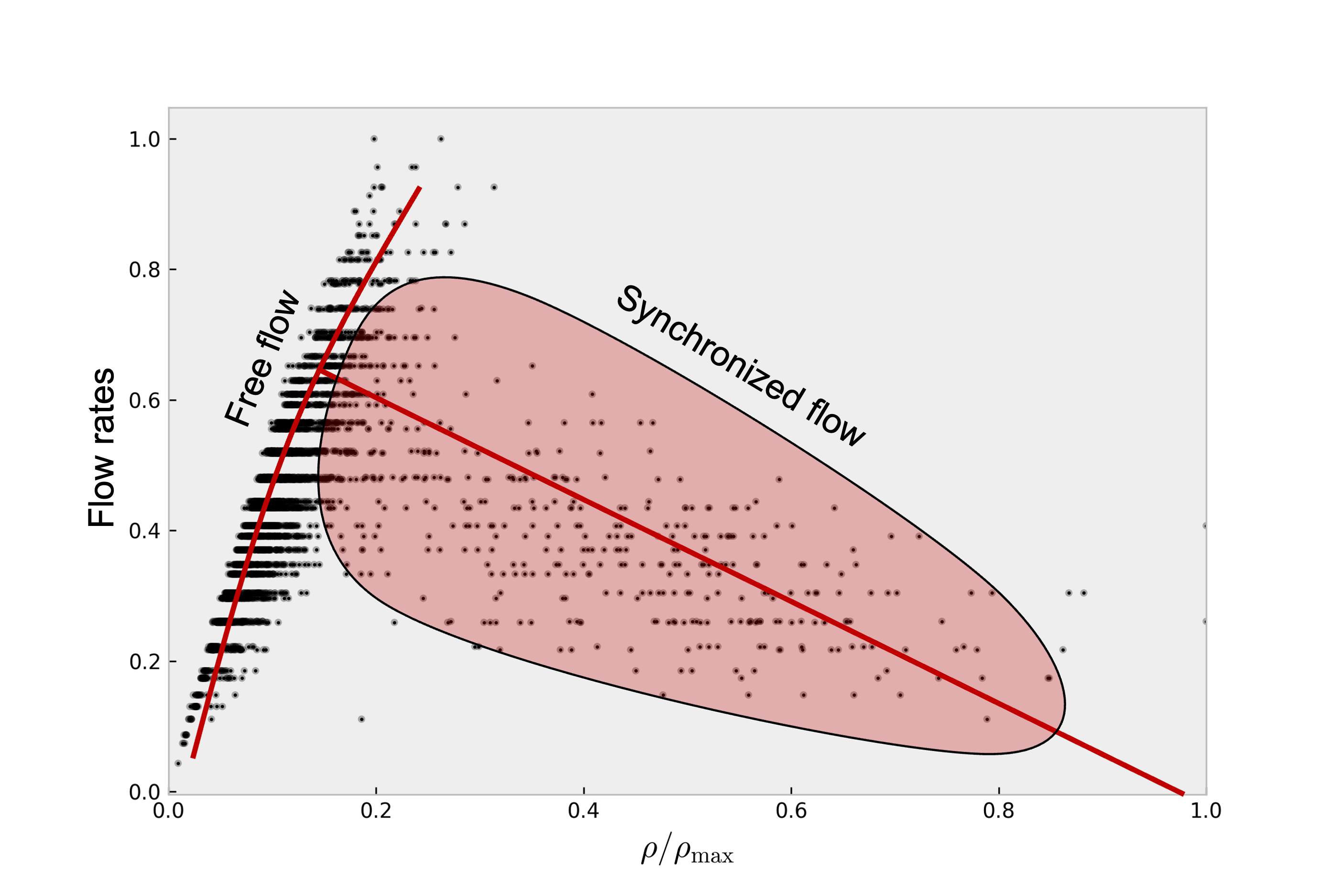
Figure 1. Example of an empirical fundamental diagram with its phases: (a) fundamental diagram, (b) decomposition of the flow in two phases.

The fundamental diagram is the plot of empirical measures of vehicle flow rate versus density. An example of a fundamental diagram obtained from a 2003 Minnesota Department of Transportation [38] database of a highway sensor is shown in Figure 1(a). In macroscopic models the fundamental diagram is approximated by a unimodal function (i.e., a function that has one extremum) $Q=Q(\rho)$. Then $Q$ is given by $Q(\rho)=\rho U(\rho)$, where $U(\rho)$ is known as the desired speed, which is a decreasing function of $\rho$ (higher vehicle density implies less freedom of movement for vehicles). In other words, the decreasing behavior of $U(\rho)$ describes drivers’ attitude to reduce speed with increasing local traffic density $\rho$.

The first fundamental diagram (FD) was measured in the 1930s by Greenshields [39] and led to the quadratic expression $Q(\rho)=u_{\max}\rho(1-\rho/\rho_{\max})$, corresponding to

$$U(\rho)=u_{\max}(1-\rho/\rho_{\max}),$$ (2.3)

where $u_{\max}$ is a maximal velocity (corresponding to a free highway) and $\rho_{\max}$ is a maximal density of cars, usualled associated with a bumper-to-bumper situation. Subsequent studies revealed that a quadratic approximation would not be adequate and numerous alternative functions have been proposed, such as piecewise linear functions [40, 41] or bi-quadratic ones [42]. Usually, the fundamental diagram is classified into two or three phases, depending on the theory. The two-phase theory divides the FD into free-flow and synchronized-flow phases, as shown in Figure 1(b). The three-phase theory identifies flow for low density (free flow), medium density (synchronized flow), or high density (moving jams) [43]. This subdivision into different regimes defines various portions of the function $Q=Q(\rho)$. An example of a function $Q(\rho)$ can be the Newell-Daganzo flow [40, 41], which corresponds to a piecewise linear flow given by

$$Q(\rho)=\begin{cases}\dfrac{Q_{\max}\rho}{\rho_{\mathrm{c}}}&\text{if $0\leq\rho<\rho_{\mathrm{c}}$},\\ Q_{\max}\left(\dfrac{\rho_{\max}-\rho}{\rho_{\max}-\rho_{\mathrm{c}}}\right)&\text{if $\rho_{\mathrm{c}}\leq\rho<\rho_{\max}$},\end{cases}$$ (2.4)

where $Q_{\max}=u_{\max}\rho_{\mathrm{c}}$ and $\rho_{\mathrm{c}}$ is the so-called critical density at which the flow is maximal. Another example is the function

$$Q(\rho)=c\left(g(0)+(g(1)-g(0))\frac{\rho}{\rho_{\max}}-g\left(\frac{\rho}{\rho_{\max}}\right)\right)\quad\text{with}\quad g(y)\coloneqq\sqrt{1+\left(\frac{y-b}{\lambda}\right)^{2}}$$ (2.5)

proposed in [3], which is a smoothed version of the Newell-Daganzo flow (2.4) and whose parameters ($c,b,\lambda$) can be adjusted by using least squares with a dataset to approximate any fundamental diagram [44]. In Figure 2(b) the various flows mentioned are compared, where we set $\rho_{\mathrm{c}}\coloneqq\rho_{\max}/3$.

(a)	(b)

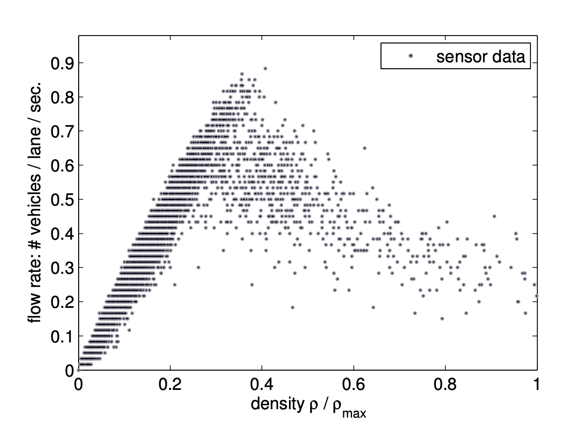
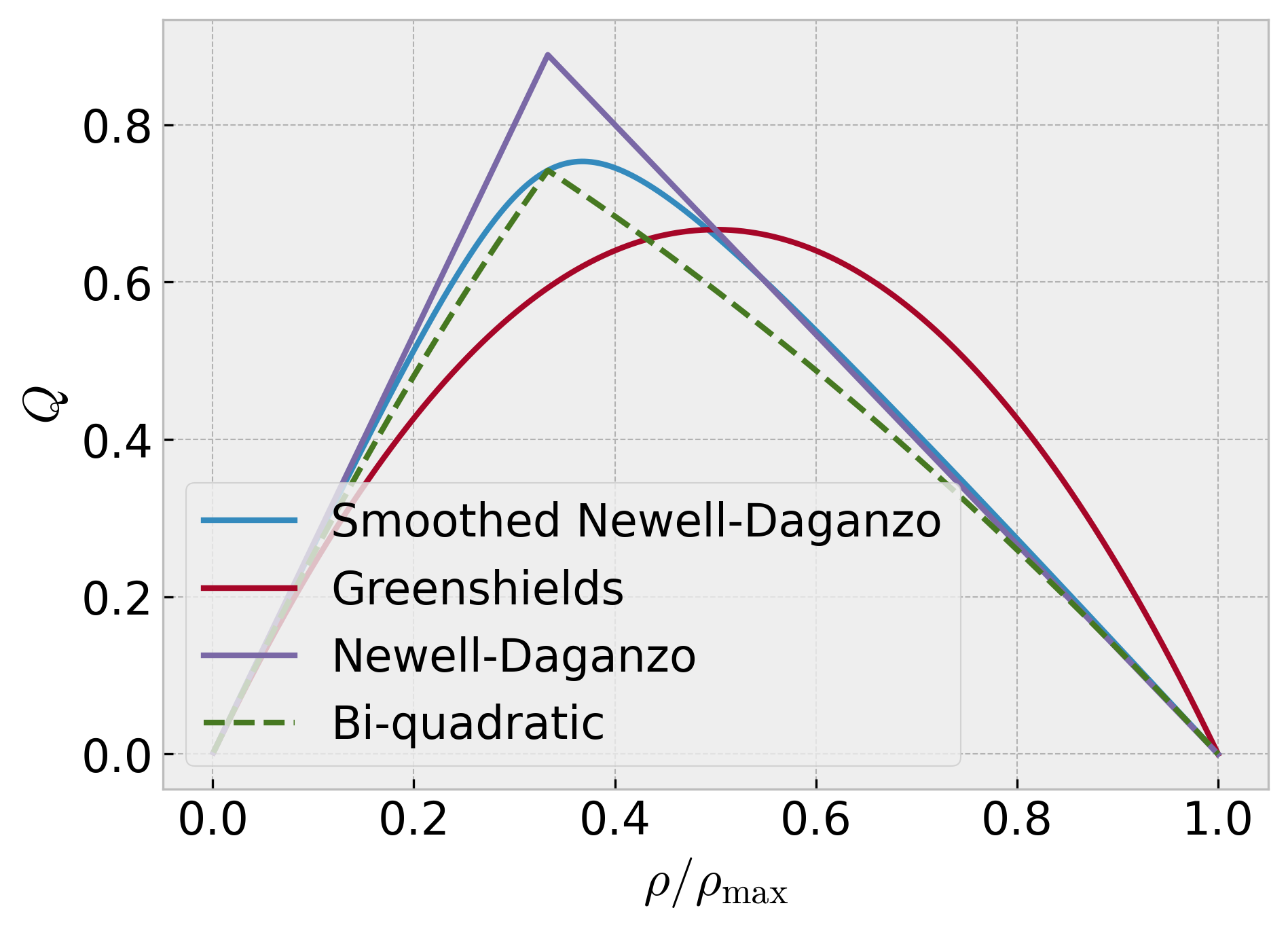
Figure 2. Fundamental diagram used in [3] and comparison of some flows: (a) fundamental diagram, (b) comparison between several different flows.

2.3. LWR model

The LWR model (or kinematic traffic model) [9, 10] is based on a fundamental relationship between $\rho$ and $u$. Let $u(\rho)=U(\rho)$, where $U(\rho)$ is defined based on the fundamental diagram. A first choice for $U$ could be (2.3). That equation interpolates linearly between the maximum speed $u_{\max}$ at which an individual vehicle can travel and the velocity zero. This choice leads to a quadratic approximation of the fundamental diagram, as seen in Figure 2(b). However, other alternatives can be defined based on flows $Q(\rho)$ that better approximate the fundamental diagram, with the relationship $U(\rho)=Q(\rho)/\rho$ (remember that $\rho>0$). The LWR model is therefore given by the scalar, nonlinear conservation law

$$\partial_{t}\rho+\partial_{x}Q(\rho)=0.$$ (2.6)

Although this model adequately describes vehicular traffic at low densities, it cannot reproduce the phenomenon of “phantom congestion” [45], which consists in the appearance of traffic jams without the influence of external factors and occurs due to the propagation of small disturbances in traffic. This latter problem is critical because traffic jams arise precisely from this phenomenon, which is the main focus of this work.

2.4. Payne-Whitham (PW) model

The Payne-Whitham (PW) model [36, 37] was the first second-order model proposed. It is given by the system

$$\begin{split}\partial_{t}\rho+\partial_{x}(\rho u)=0,\qquad\partial_{t}u+u\partial_{x}u+\dfrac{1}{\rho}\partial_{x}p(\rho)=\dfrac{U(\rho)-u}{\tau},\end{split}$$ (2.7)

where $p(\rho)$ is a strictly increasing function and (the “traffic pressure”) that models preventive driving, and $\tau$ is the relaxation time representing the time it takes for drivers to adjust their speed to the desired speed. Possible choices include the so-called “regular pressure” $p(\rho)\coloneqq\beta\rho^{\gamma}$ with coefficients $\beta,\gamma>0$ or the more complicated so-called “singular pressure”

$$p(\rho)=-\beta\left(\dfrac{\rho}{\rho_{\max}}+\ln\left(1-\dfrac{\rho}{\rho_{\max}}\right)\right).$$ (2.8)

In [3], it is proved that the PW model has solutions governed by self-sustained nonlinear traveling waves (jamitons). However, the PW model has been criticized in [46] because, under certain conditions, it admits solutions with negative flows and velocities (vehicles moving in the direction of decreasing $x$). For this reason other second-order traffic models are preferred, although they maintain the relaxation term in the second equation.

2.5. The inhomogeneous ARZ model

The inhomogeneous ARZ model [6, 7] given by (1.1) modifies the PW model (2.7). Instead of a pressure function (such as (2.8)) it involves a so-called hesitation function $h=h(\rho)$, which is assumed to be strictly increasing and plays a role similar to pressure in the PW model. The model (1.1) is a hyperbolic system of conservation laws with a relaxation term. It had originally been proposed in its homogeneous version, but the addition of the relaxation term in the second equation is precisely the ingredient that allows the appearance of jamitons. The functions $U=U(\rho)$ and $h=h(\rho)$ are assumed to be twice differentiable and satisfy the following conditions:

1. The function $U$ satisfies $U^{\prime}(\rho)<0$ and $U^{\prime\prime}(\rho)>0$, hence $U(\rho)$ is decreasing and $Q(\rho)$ is concave since $Q^{\prime\prime}(\rho)=2U^{\prime}(\rho)+U^{\prime\prime}(\rho)>0$.

2. The function $h$ satisfies $h^{\prime}(\rho)>0$ and $\mathrm{d}^{k}(\rho h(\rho))/\mathrm{d}\rho^{k}>0$, $k=1,2$.

These two assumptions ensure that the equations are well posed in the presence of jump-type solutions. In [6], it is proven that the system (1.1) is indeed hyperbolic. This is done by multiplying first equation of (1.1) by $h^{\prime}(\rho)$ and subtracting the result from the second, which yields the system

$$\begin{split}\partial_{t}\rho+\partial_{x}(\rho u)&=0,\\ \partial_{t}u_{t}+\bigl{(}u-\rho h^{\prime}(\rho)\bigr{)}\partial_{x}u&=\frac{h^{\prime}(\rho)}{\tau}\bigl{(}U(\rho)-u\bigr{)}.\end{split}$$ (2.9)

We define

$$\bm{w}\coloneqq\begin{pmatrix}\rho\\ u\end{pmatrix},\quad\bm{L}(\bm{w})\coloneqq\begin{pmatrix}u&\rho\\ 0&u-\rho h^{\prime}(\rho)\end{pmatrix},\quad\bm{f}(\bm{w})\coloneqq\begin{pmatrix}0\\ \dfrac{h^{\prime}(\rho)}{\tau}(U(\rho)-u)\end{pmatrix}$$ (2.10)

to write the linearized ARZ system (2.9) as

$$\partial_{t}\bm{w}+\bm{L}(\bm{w})\partial_{x}\bm{w}=\bm{f}(\bm{w}).$$ (2.11)

The eigenvalues of the matrix $\bm{L}(\bm{w})$ are given by

$$\lambda_{1}=u-\rho h^{\prime}(\rho),\quad\lambda_{2}=u,$$ (2.12)

which, according to assumption ((b)), satisfy $\lambda_{1}<\lambda_{2}$ if $\rho>0$. Therefore, the system (1.1) is strictly hyperbolic. The eigenvalues of the system are known as characteristic speeds and describe conditions for the existence of jamitons. Depending on the variables defined, the ARZ model (2.11) may be formulated in two other ways, namely either in conservative or in Lagrangian form.

The conservative form is achieved if we define the variable $y\coloneqq\rho(u+h(\rho))$, which implies $u=y/\rho-h(\rho)$. Substituting this into the first equation of (1.1) yields

$$\partial_{t}\rho+\partial_{x}\bigl{(}y-\rho h(\rho)\bigr{)}=0.$$

For the second relationship, the first equation of (1.1) is multiplied by $(u+h(\rho))$ and added to the second equation of (1.1) multiplied by $\rho$, which results in the system in Eulerian variables

$$\partial_{t}\rho+\partial_{x}(\rho u) =0,$$

$$\partial_{t}\bigl{(}\rho(u+h(\rho))\bigr{)}+\partial_{x}\bigl{(}u\rho(u+h(\rho))\bigr{)} =\frac{\rho}{\tau}\bigl{(}U(\rho)-u\bigr{)}.$$

Written in conservative variables $\bm{Q}\coloneqq(\rho,y)^{\mathrm{T}}$, this system reads

$$\begin{split}\partial_{t}\rho+\partial_{x}\bigl{(}y-\rho h(\rho)\bigr{)}&=0,\\ \partial_{t}y+\partial_{x}\left(\dfrac{y^{2}}{\rho}-yh(\rho)\right)&=\frac{1}{\tau}\bigl{(}\rho\left(U(\rho)+h(\rho)\right)-y\bigr{)}.\end{split}$$ (2.13)

Defining

$$\bm{F}(\bm{Q})\coloneqq\begin{pmatrix}y-\rho h(\rho)\\[3.0pt] \dfrac{y^{2}}{\rho}-yh(\rho)\end{pmatrix},\quad\bm{S}(\bm{Q})\coloneqq\begin{pmatrix}0\\ \dfrac{1}{\tau}\left(\rho\left(U(\rho)+h(\rho)\right)-y\right)\end{pmatrix},$$ (2.14)

we may rewrite the system (2.13) as

$$\partial_{t}\bm{Q}+\partial_{x}\bm{F}(\bm{Q})=\bm{S}(\bm{Q}).$$ (2.15)

This form will be essential for numerical simulations in forthcoming sections, as well as being useful for calculating the characteristic velocities (2.12) through the Jacobian matrix $\bm{J}_{\bm{F}}$ of $\bm{F}$.

To write the ARZ model (1.1) in Lagrangian form [47, 48] we define the variables $v(\sigma,t)$ and $u(\sigma,t)$, where $v\coloneqq 1/\rho$ and $\sigma$ satisfies

$$\mathrm{d}\sigma=\rho\,\mathrm{d}x-\rho u\,\mathrm{d}t,\quad\sigma(t=0)=\sigma_{0}~\hbox{given}.$$

In terms these variables, the model (1.1) can be written as

$$\begin{split}\partial_{t}v&=\partial_{\sigma}u,\\ \partial_{t}\bigl{(}u+\hat{h}(v)\bigr{)}&=\dfrac{\hat{U}(v)-u}{\tau},\end{split}$$ (2.16)

where $\hat{h}(v)\coloneqq h(1/v)$ and $\hat{U}(v)\coloneqq U(1/v)$ satisfy

$$\dfrac{\mathrm{d}\hat{U}}{\mathrm{d}v}>0,\quad\dfrac{\mathrm{d}^{2}\hat{U}}{\mathrm{d}v^{2}}<0,\quad\dfrac{\mathrm{d}\hat{h}}{\mathrm{d}v}<0,\quad\text{ and }\quad\dfrac{\mathrm{d}^{2}\hat{h}}{\mathrm{d}v^{2}}>0.$$

This formulation is useful for the theoretical construction of jamitons, as well as for the Smoothed Particle Hydrodynamics (SPH) method (see [49, 50]) for numerical simulations (as in [2], but the SPH method is not used herein). Both forms have associated Rankine-Hugoniot (jump) conditions. If $[\![u]\!]\coloneqq u^{+}-u^{-}$ denotes value of the jump of a variable $u$ across a discontinuity and $s$ is the jump propagation velocity, then the jump condition for (2.15) is $[\![\bm{F}(\bm{Q})]\!]=s[\![\bm{Q}]\!]$, which for Eulerian variables means that

$$\begin{split}[\![y-\rho h(\rho)]\!]&=s[\![\rho]\!],\\ [\![y^{2}/\rho-yh(\rho)]\!]&=s[\![y]\!]\end{split}$$ (2.17)

or equivalently, if we recall that $y=\rho(u+h(\rho))$ and use (2.17),

$$\begin{split}[\![\rho u]\!]&=s[\![\rho]\!],\\ [\![\rho u^{2}+\rho uh(\rho)]\!]&=s[\![\rho(u+h(\rho))]\!].\end{split}$$ (2.18)

In Lagrangian form, conditions (2.18) are replaced by

$$\begin{split}[\![u]\!]&=m[\![v]\!],\\ [\![u]\!]&=-[\![\hat{h}(v)]\!],\end{split}$$ (2.19)

where $-m$ is the jump propagation velocity but in Lagrangian variables (in the Eulerian scheme, $m$ represents the traffic flow passing through a jump). In Section 4 the relation between both quantities $s$ and $m$ is established.

2.6. Sub-characteristic condition

The macroscopic models share a type of solution called a steady state where $\rho(x,t)=\tilde{\rho}=\text{const.}$ and $u(x,t)=\tilde{u}=\text{const.}$. This means that the traffic flows uniformly: vehicles always keep the same distance from each other and move at their desired speed $\tilde{u}=U(\tilde{\rho})$. On the other hand, the relaxation term introduced in second-order models causes the traffic velocity $u$ to converge to $U(\rho)$ as $\tau\to 0^{+}$. In this case, the solutions of the ARZ and PW models are dominated by the continuity equation (2.2) with $u=U(\rho)$, which precisely corresponds to the LWR model. Also note that the characteristic velocity of the LWR model is given by

$$\mu(\rho)=Q^{\prime}(\rho)=\rho U^{\prime}(\rho)+U(\rho).$$ (2.20)

Let $\rho(x,t)=\tilde{\rho}\geq 0$ and $u(x,t)=\tilde{u}=U(\tilde{\rho})$ denote a base state for some second-order model. We say that the base state $(\tilde{\rho},\tilde{u})$ is linearly stable if any small perturbation decays over time. On the other hand, the base state $(\tilde{\rho},\tilde{u})$ is said to satisfy the sub-characteristic condition (SCC) if the characteristic velocity $\mu=\mu(\tilde{\rho})$ defined by (2.20) for $\rho=\tilde{\rho}$ lies between the two characteristic velocities $\lambda_{1}=\lambda_{1}({\tilde{\rho},\tilde{u}})$, $\lambda_{2}=\lambda_{2}({\tilde{\rho},\tilde{u}})$ with $\lambda_{1}<\lambda_{2}$ of the second-order model, that is:

$$\lambda_{1}<\mu<\lambda_{2}.$$ (2.21)

The previous concepts may be considered different, but actually Whitham’s theorem proven in [51] relates both:

Theorem 2.1 (Whitham [51]).

The base state $(\tilde{\rho},\tilde{u})$ is linearly stable if and only if it satisfies the sub-characteristic condition (2.21).

Since second-order models are capable of reproducing traffic instabilities, Whitham’s theorem is crucial for distinguishing between stable and unstable base states more easily through the SCC. Nonetheless, instabilities can be directly studied by calculating the growth factor for perturbations of the form $\mathrm{e}^{\mathrm{i}kx}$, as is done in [52], where the same SCC inequality (2.21) is obtained.

For the ARZ model, the characteristic speeds are given by (2.12), so its SCC (2.21) corresponds to

$$\tilde{u}-\tilde{\rho}h^{\prime}(\tilde{\rho})<\tilde{\rho}U^{\prime}(\tilde{\rho})+U(\tilde{\rho})<\tilde{u},$$

but $\tilde{u}=U(\tilde{\rho})$, so we obtain

$$-\tilde{\rho}h^{\prime}(\tilde{\rho})<\tilde{\rho}U^{\prime}(\tilde{\rho})<0.$$

By assumption ((a)), the second inequality always holds. Thus, it follows that for the ARZ model the base state $(\tilde{\rho},\tilde{u})$ is linearly stable if and only if $-\tilde{\rho}h^{\prime}(\tilde{\rho})<\tilde{\rho}U^{\prime}(\tilde{\rho})$ or equivalently,

$$h^{\prime}(\tilde{\rho})+U^{\prime}(\tilde{\rho})>0.$$

2.7. Some remarks on Whitham’s theorem

Theorem 2.1 has been investigated and extended in several works [53, 54, 55, 51, 37], with a primary focus on the SCC and on even more general $N$-equation hyperbolic systems than traffic models. These results include the following findings. We first mention that Theorem 2.1 can be extended to relate the SCC to the stability of solutions, in the sense that a steady-state solution with small perturbations converges to the initial steady state as $t\to\infty$. Furthermore, solutions to second-order models that satisfy the SCC everywhere converge to LWR solutions as $\tau\to 0$. More generally, if $\tau$ is not small enough, solutions to second-order models converge to LWR solutions but with an additional nonlinear viscosity term of magnitude $\mathcal{O}(\tau)$. Finally, dedicated analyses of the degenerating cases of the SCC (corresponding to the situation when $\lambda_{1}=\mu<\lambda_{2}$ or $\lambda_{1}<\mu=\lambda_{2}$) are available [56, 57].

An interesting question that has been studied in [3, 2, 52] is the following: how do the solutions close to constant base states evolve in second-order models when the SCC is not satisfied? In the mentioned works and in numerical studies [2, 47], it is shown that these solutions converge to regimes dominated by jamitons, which will be the main focus of this work.

3. Jamitons

In this section we describe in detail the construction of jamitons as exact solutions to the ARZ model. We closely follow the approach by Ramadan [58].

3.1. Model functions

The results of the analysis are illustrated in a series of plots that are based on the following specific functions for the ARZ model (1.1). We assume that the function $Q=Q(\rho)$ is given by (2.5) with parameters $b=1/3$, $c=0.078u_{\max}\rho_{\max}$, $\lambda=1/10$, and $u_{\max}=20\,\mathrm{m}\mathrm{s}^{-1}$, chosen to fit real data [3]. The value of $\rho_{\max}$ is based on assuming a length of $5\,\mathrm{m}$ per vehicle plus an extra $50\%$ of safety distance between them. Then, at $\rho_{\max}$ there will be exactly one vehicle each $7.5$ meters, and therefore $\rho_{\max}=(1/7.5)\,\mathrm{m}^{-1}$. The desired velocity is given by $U(\rho)=Q(\rho)/\rho$, and the hesitation function is

$$h(\rho)=\beta\left(\frac{\rho}{\rho_{\max}-\rho}\right)^{\gamma}\quad\text{with $\beta=8$ and $\gamma=1/2$}.$$

The relaxation time $\tau$ for testing and obtaining general results will be $\tau=5$ seconds, but in Section 5, effects for other values of $\tau$ will be studied. The plots of the functions are presented in Figure 3.

(a)	(b)
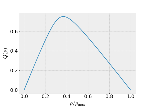
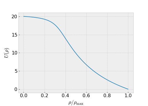
(c)	(d)

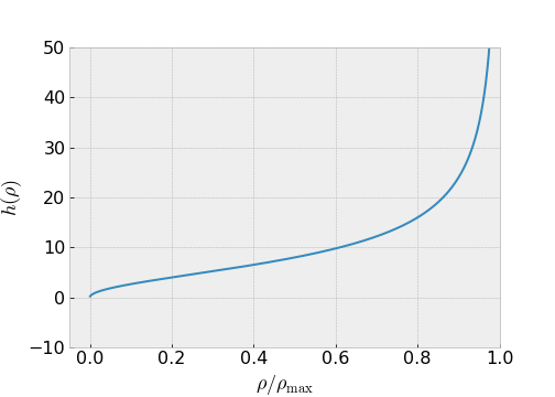
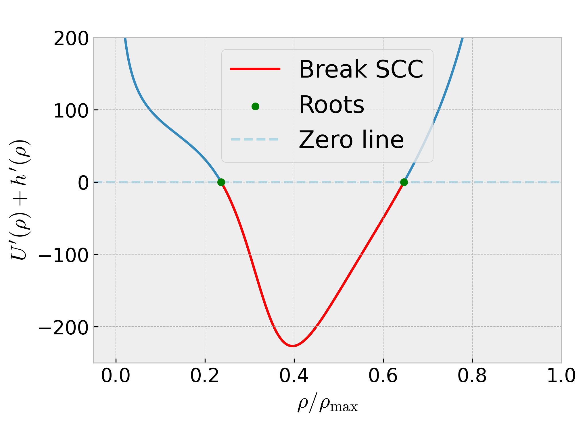
Figure 3. Plots of functions defined in section 3.1: (a) flow $Q(\rho)$, (b) desired velocity $U(\rho)$, (c) hesitation function $h(\rho)$, (d) plot of $U^{\prime}(\rho)+h^{\prime}(\rho)$ illustrating the interval of violation of the SCC for the corresponding ARZ model.

3.2. Traveling-wave analysis

Jamitons are defined as self-sustained traveling waves that arise in second-order models. These can be constructed following the Zel’dovich-von Neumann-Döring (ZND) theory [59] since they have the same mathematical structure as detonation waves. A traveling-wave approach leads to obtain an expression for jamitons. The construction is based the Lagrangian formulation (2.16), but the final expressions and simulations will be translated to Eulerian variables for better physical visualization. Let

$$\chi\coloneqq\frac{mt+\sigma}{\tau}.$$

The goal is to find traveling-wave solutions $v(\sigma,t)=v(\chi)$ and $u(\sigma,t)=u(\chi)$ of (2.16). Substituting these expressions into (2.16) yields the system of equations

$$\frac{m}{\tau}v^{\prime}(\chi)-\frac{1}{\tau}u^{\prime}(\chi) =0,$$ (3.1)

$$\frac{m}{\tau}u^{\prime}(\chi)+\hat{h}^{\prime}(v(\chi))\frac{m}{\tau}v^{\prime}(\chi) =\frac{\hat{U}(v(\chi))-u(\chi)}{\tau}.$$ (3.2)

Directly integrating equation (3.1), one obtains

$$mv-u=-s,$$ (3.3)

where $s$ is an integration constant. In Lagrangian variables, $-m$ corresponds to the propagation speed of the jamiton, while $s$ corresponds to the flow of vehicle mass passing through the wave. In Eulerian variables, both constants interchange their meanings ($s$ corresponds to speed and $-m$ to mass flow). Equation (3.3) implies that

$$u=s+mv,$$ (3.4)

and replacing (3.4) in (3.2) yields the ODE of the jamiton:

$$v^{\prime}(\chi)=\dfrac{w(v(\chi))}{r^{\prime}(v(\chi))},\quad\text{where $w(v)=\hat{U}(v)-(mv+s)$ and $r(v)=m\hat{h}(v)+m^{2}v$. }$$ (3.5)

Since $\hat{h}^{\prime}(v)<0$ and $\hat{h}^{\prime\prime}(v)>0$, the function $r^{\prime}(v)$ has at most one root $v_{s}$, i.e., $r^{\prime}(v_{s})=0$ or equivalently, $\hat{h}^{\prime}(v_{s})=-m$. The ODE (3.5) can then be integrated across $v_{s}$ if $w(v)$ has one root at $v_{s}$ as well, that is $w(v_{s})=0$ or equivalently,

$$\hat{U}(v_{s})=mv_{s}+s.$$ (3.6)

Equation (3.6) is known as the Chapman-Jouguet condition in ZND theory, and the point $v_{s}$ is called the sonic point. Then, smooth traveling wave solutions of the ODE (3.5) can be parametrized by $v_{s}$, the sonic point, where the constants $m$ and $s$ are given by

$$m=-\hat{h}^{\prime}(v_{s})\quad\text{ and }\quad s=\hat{U}(v_{s})-mv_{s}.$$ (3.7)

Jumps moving at velocity $-m$ can be added to the smooth profile found using the Rankine-Hugoniot conditions (2.19). The first condition in (2.19), $[\![u]\!]=m[\![v]\!]$, states that the quantity $mv-u$ is conserved across a jump, which corresponds to condition (3.4) for the smooth part of the traveling wave. Combining both conditions in (2.19) and multiplying the result by $m$ yields

$$[\![r(v)]\!]=[\![m^{2}v+\hat{h}(v)]\!]=0;$$

in other words, $r(v)$ is conserved across a jump. Then, by integrating (3.5) one can incorporate a jump at some value $v^{-}$ that jumps to a value $v^{+}$ such that $r(v^{-})=r(v^{+})$ and continue integrating from there. Moreover, a necessary condition for the jump to satisfy the Lax entropy conditions is that the specific volume must decrease through the jump, i.e., $v^{+}<v_{s}<v^{-}$, so the smooth portion of the jamiton profile $v(\chi)$ must be increasing. Applying L’Hospital’s rule to the solution of (3.5) at the point $v_{s}$ and keeping in mind that $v$ must be increasing, we obtain that

$$\dfrac{\hat{U}^{\prime}(v_{s})+\hat{h}^{\prime}(v_{s})}{-\hat{h}^{\prime}(v_{s})\hat{h}^{\prime\prime}(v_{s})}>0,$$

that is, $\hat{U}^{\prime}(v_{s})+\hat{h}^{\prime}(v_{s})>0$ and therefore the SCC does not hold at $v_{s}$, so jamitons with jumps exist if and only if the SCC is violated. Consequently, since $w^{\prime\prime}(v)=\hat{U}^{\prime\prime}(v)<0$ always and $w^{\prime}(v)>0$ for $v<v_{s}$, the function $w$ may have a second root $v_{M}$ only for $v>v_{s}$, and since (3.5) cannot be integrated beyond $v_{M}$, this profile corresponds to a maximal jamiton connecting the points $v_{M}$ with $v_{R}$, where $r(v_{R})=r(v_{M})$. It should be noted that the appearance of a maximal jamiton is purely theoretical as it is infinitely long. The same procedure can be carried out in Eulerian variables for (2.13) by defining $\eta\coloneqq(x-st)/\tau$. If we compare this with the kink solution (1.3) of the $\phi^{4}$ equation (1.2), then the same profile behavior in Eulerian variables is obtained. In the case of jamitons, however, an explicit formula is not available, but the traveling-wave behavior is preserved.

(a)	(b)

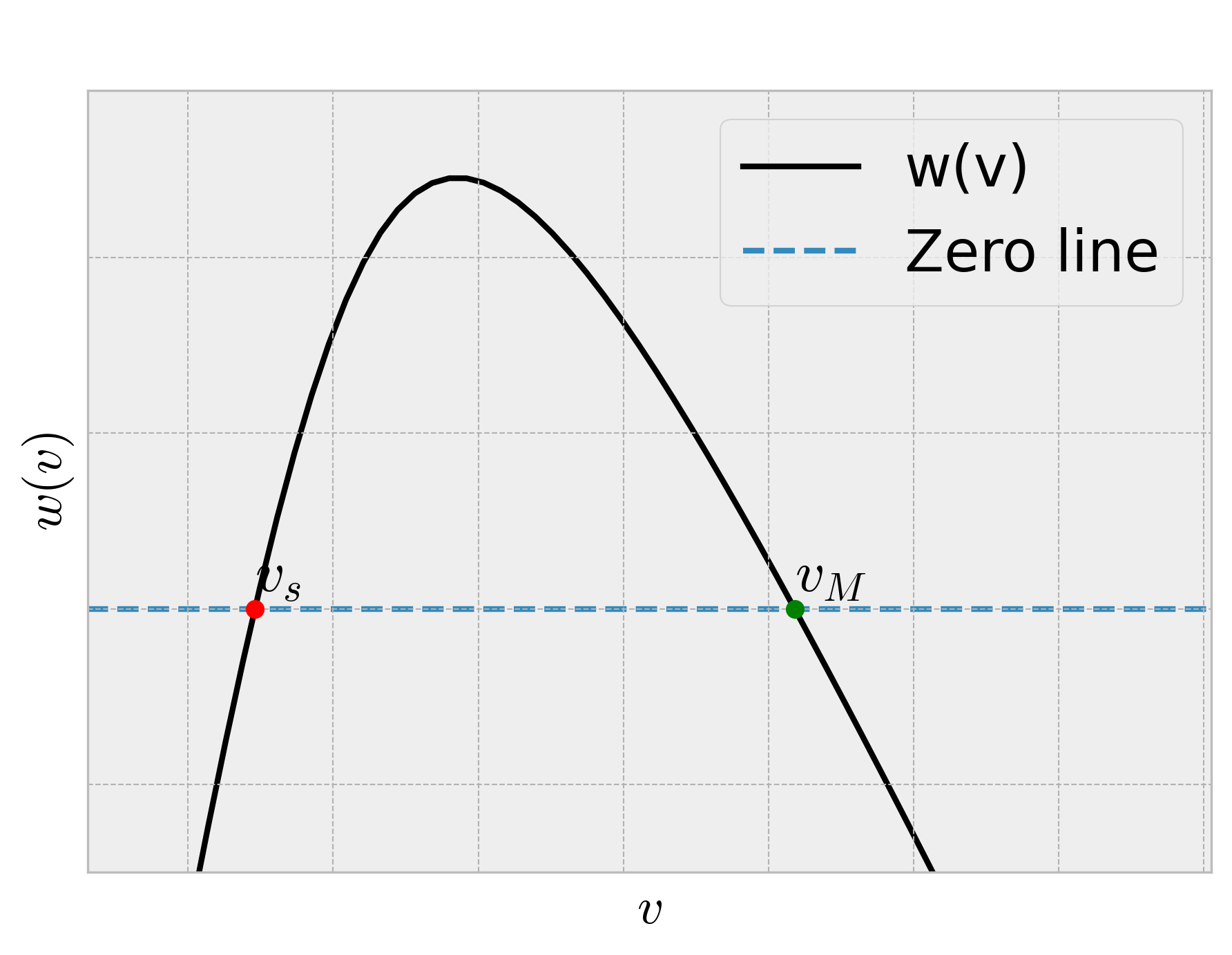
Figure 4. Functions $w$ and $r$ with a maximal jamiton and an example of standard jamiton: (a) function $w(v)$ with a second root $v_{M}$, (b) function $r(v)$ with a maximal jamiton and an example of other jamiton. The point $v_{s}$ corresponds to the minimum of $r$.

3.3. Construction of jamitons

Based on the previously discussed theoretical aspects, jamitons can be constructed as follows [58]:

1. Choose $\rho_{s}$ that does not satisfy the SCC condition and define $v_{s}\coloneqq 1/\rho_{s}$.

2. Define $m\coloneqq-h^{\prime}(v_{s})$ and $s\coloneqq U(v_{s})-mv_{s}$.

3. Look for $v_{M}>v_{s}$ such that $w(v_{M})=0$ and define $r_{\min}\coloneqq r(v_{s})$ and $r_{\max}\coloneqq r(v_{M})$ (see Figure 4).

4. Search for $v_{R}<v_{s}$ such that $r(v_{R})=r_{\max}$.

5. Choose $v^{-}$ such that $v_{s}<v^{-}$ and $r(v^{-})\in(r_{\min},r_{\max})$.

6. Choose $v^{+}$ such that $v^{+}<v_{s}$ and $r(v^{-})=r(v^{+})$.

7. One solves the initial-value problem of the ODE (3.5) from a point $\chi_{\mathrm{start}}$ with initial condition $v(\chi_{\mathrm{start}})=v^{+}$ and stops when the value $v^{-}$ is reached.

(a)	(b)

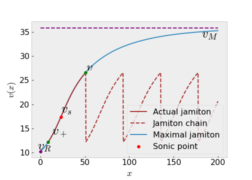
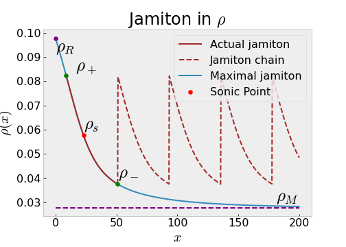
(c)

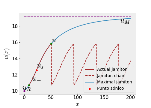
Figure 5. Example of a chain of jamitons, along with a maximal jamiton, shown as a function (a) $v=v(x)$, with jamitons between $v^{+}$ and $v^{-}$, (b) $\rho=\rho(x)$, with jamitons between $\rho^{+}$ and $\rho^{-}$, (c) $u=u(x)$, with jamitons between $u^{+}$ and $u^{-}$.

(a)

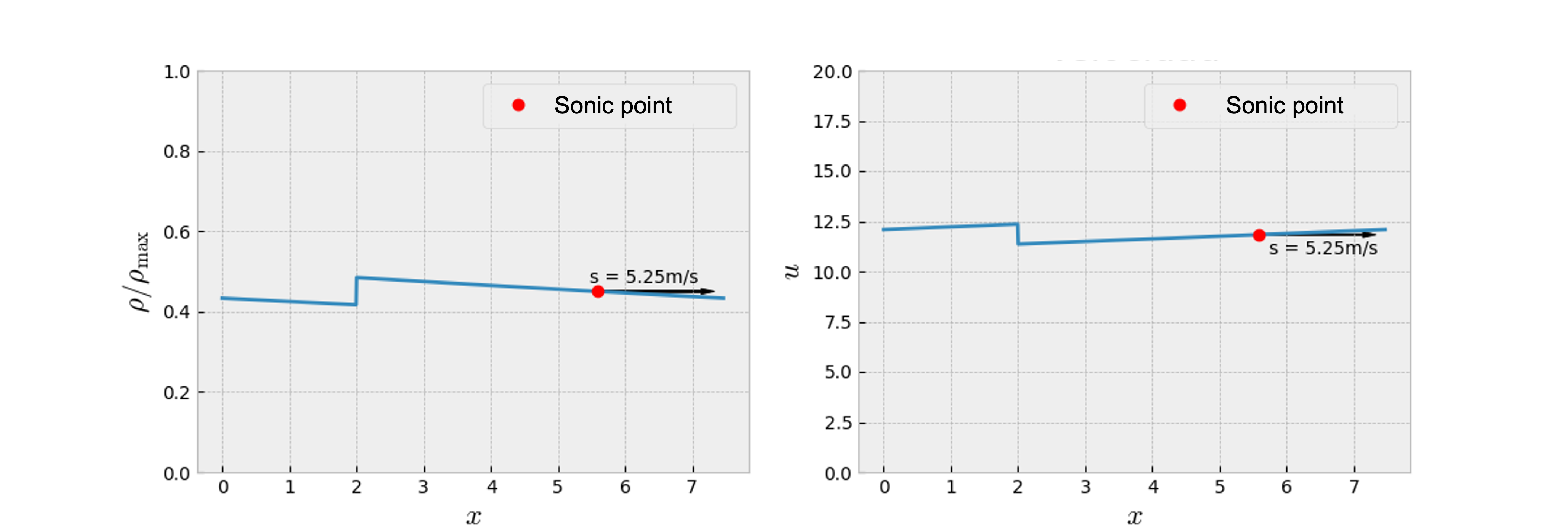
(b)

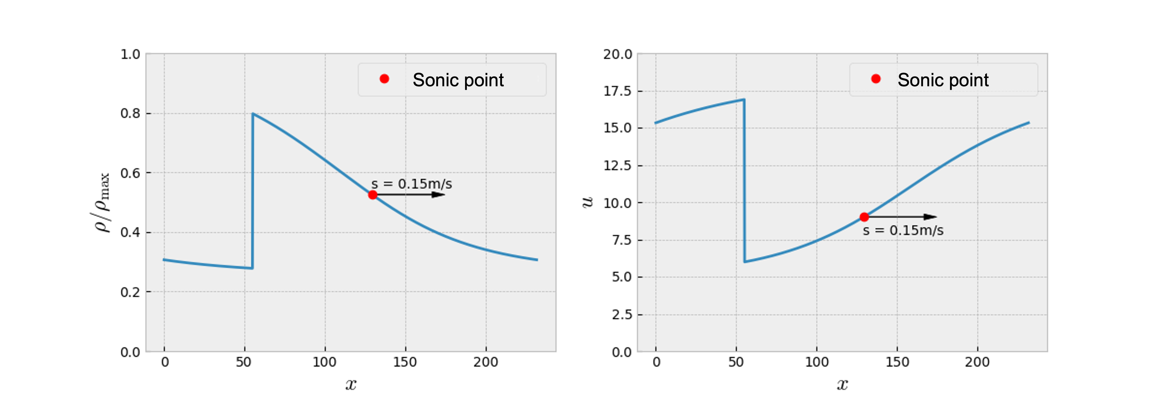
(c)

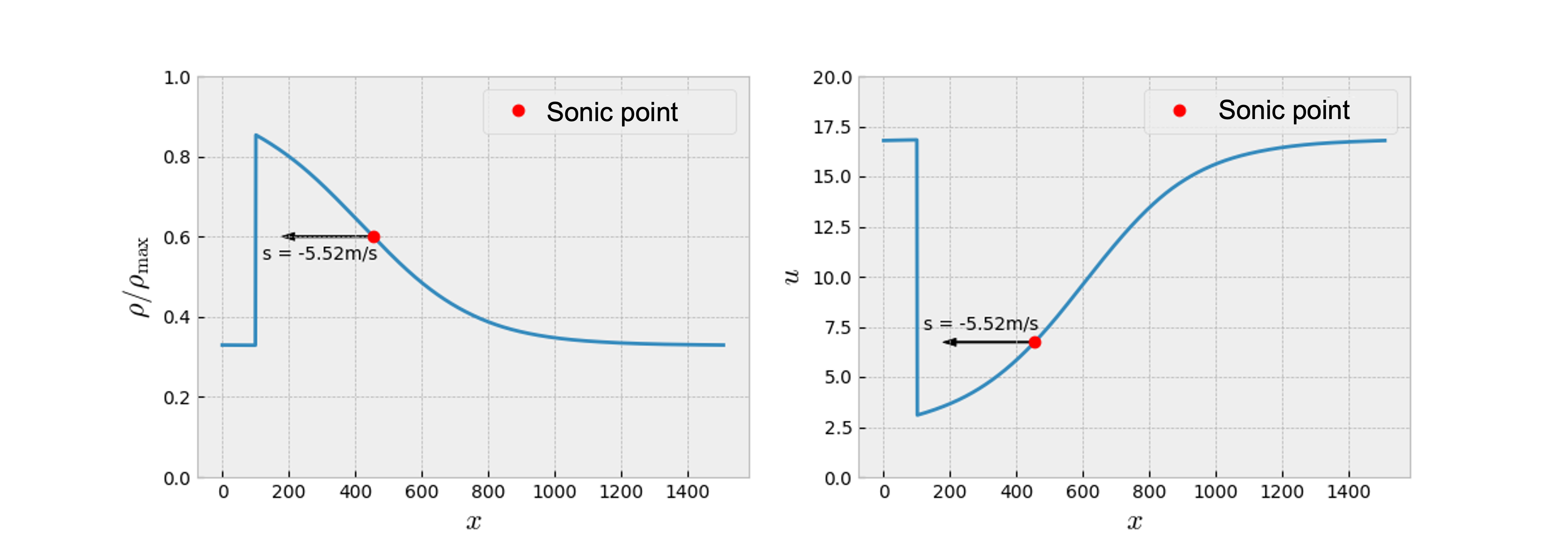
Figure 6. Jamitons of various lengths: (a) small-length jamiton with $\rho_{s}=0.45\rho_{\max}$, with length $L\approx 15.27$ and $N\approx 0.91$ vehicles, (b) medium-length jamiton with $\rho_{s}=0.525\rho_{\max}$, $L\approx 231.70$ and $N\approx 14.05$ (notice that this jamiton moves to the left), (c) long jamiton with $\rho_{s}=0.6\rho_{\max}$, $L\approx 1507.27$ and $N\approx 93.65$, shown in all cases in the variables (left) $\rho$ and (right) $u$.

In Figure 5, examples of jamitons in the variables $v$, $\rho$, and $u$ are presented, where we recall that $v=1/\rho$ and $u$ is obtained from (3.4). In such cases, integration was performed in the variable $x$, where we used that

$$\mathrm{d}\eta=\frac{1}{\tau}(x-s\,\mathrm{d}t)=\frac{1}{\tau}(\mathrm{d}x+mv\,\mathrm{d}t-u\,\mathrm{d}t)=\frac{1}{\tau}(v\,\mathrm{d}\sigma+mv\,\mathrm{d}t)=v\,\mathrm{d}\chi,$$

and the chain rule in the ODE (3.5). With this construction, some properties of the jamiton in the coordinate $x$ can be calculated, such as its length $L$ given by

$$L=\tau\int_{v^{+}}^{v^{-}}v\dfrac{r^{\prime}(v)}{w(v)}\,\mathrm{d}v,$$ (3.8)

the total number $N$ of vehicles [3] in the jamiton given by

$$N=\tau\int_{v^{+}}^{v^{-}}\dfrac{r^{\prime}(v)}{w(v)}\,\mathrm{d}v,$$ (3.9)

and its amplitude $A$ defined by

$$A=\rho_{+}-\rho_{-}.$$ (3.10)

In Figure 6 jamitons of various sizes and speeds are shown, along with their lengths (3.8) and total numbers of vehicles (3.9). In this case, the number of vehicles may not be natural since it is a continuous model, but an approximate value is obtained.

3.4. Jamitons in the fundamental diagram

(a)	(b)

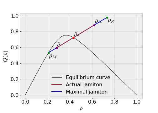
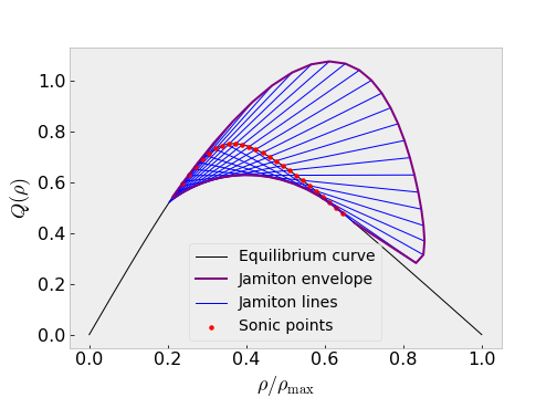
Figure 7. Illustration of jamitons in the fundamental diagram: (a) maximal jamiton and a jamiton in the $(\rho,q)$-plane (both lie on the same line passing through $(\rho_{s},Q(\rho_{s}))$), (b) jamiton region composed of several maximal jamitons, along with the jamitonic envelope.

It is instructive to visualize jamitons in the fundamental diagram. Roughly speaking, the idea consists in visualizing all pairs $(\rho,q\coloneqq\rho u)$ that arise within the definition of one jamiton. Clearly, since jamitons are not constant solutions, they cannot be points on the FD. By multiplying the relationship (3.4) by $\rho$, one has

$$q=\rho u=s\rho+m,$$ (3.11)

in other words, a jamiton gives rise to a line segment in the $(\rho,q)$-plane of flow rate versus density, and its slope corresponds to the propagation speed of the jamiton. Furthermore, using the Chapman-Jouguet condition (3.6) for $v_{s}=1/\rho_{s}$ and the equalities (3.7), we may rewrite (3.11) as

$$q=s(\rho-\rho_{s})+\rho_{s}U(\rho_{s})$$ (3.12)

and evaluating (3.12) at $\rho=\rho_{s}$, we obtain that $q(\rho_{s})=\rho_{s}U(\rho_{s})=Q(\rho_{s})$ by definition of $Q$, and therefore, the jamiton segment intersects the equilibrium flow at $\rho_{s}$. In Figure 7, an example of a jamiton in the fundamental diagram is depicted, where the endpoints of the segment $(\rho^{+},\rho^{+}u^{+})$ and $(\rho^{-},\rho^{-}u^{-})$ represent the two states of the jamiton across the jump.

For each $\rho_{s}$ that violates the SCC, the corresponding maximal jamiton is the line segment connecting the points $(\rho_{M},m+s\rho_{M})$ and $(\rho_{R},m+s\rho_{R})$, where $\rho_{M}=1/v_{M}$ and $\rho_{R}=1/v_{R}$ are constructed following the steps in Section 3.3. Since $w(v_{M})=0$ by construction, there holds $\smash{\hat{U}(v_{M})=mv_{M}+s}$, and multiplying this identity by $\rho_{M}$ yields $m+s\rho_{M}=Q(\rho_{M})$, hence $(\rho_{M},m+s\rho_{M})$ also belongs to the equilibrium curve. Figure 7 shows some maximal jamitons for various $\rho_{s}$ that violate the SCC, along with the jamitonic envelope. This envelope indicates the boundary on which the jamitons must fall, called the jamiton region. The upper envelope corresponds to the curve generated by joining the points $(\rho_{R},m+s\rho_{R})$. On the other hand, the segments of jamitons also intersect below the equilibrium line, so they also form a lower envelope. This curve is given by points $(\rho^{*},q^{*})$ that satisfy

$$\rho^{*}(\rho_{s})=-\frac{m^{\prime}(\rho_{s})}{s^{\prime}(\rho_{s})},\quad q^{*}(\rho_{s})=m(\rho_{s})+s(\rho_{s})\rho^{*}(\rho_{s}).$$

An interesting result proven in [3, 52] is that the velocity of a jamiton is determined by the sonic density $\rho_{s}$ only. Furthermore, $s$ decreases with respect to $\rho_{s}$. Indeed, from (3.7) written in Eulerian variables, we deduce that

$$s(\rho_{s})=U(\rho_{s})-\rho_{s}h^{\prime}(\rho_{s}),$$

hence

$$s^{\prime}(\rho_{s})=U^{\prime}(\rho_{s})-h^{\prime}(\rho_{s})-\rho_{s}h^{\prime\prime}(\rho_{s})=U^{\prime}(\rho_{s})+h^{\prime}(\rho_{s})-\bigl{(}\rho_{s}h(\rho_{s})\bigr{)}^{\prime\prime}.$$

We have $U^{\prime}(\rho_{s})+h^{\prime}(\rho_{s})<0$ since it is assumed that $\rho_{s}$ violates the SCC (if not, there would be no jamiton), while $(\rho_{s}h(\rho_{s}))^{\prime\prime}>0$ since it was assumed that $\rho h(\rho)$ is convex. Thus, $s^{\prime}(\rho_{s})<0$, i.e., $s$ decreases with respect to $\rho_{s}$. Figure 7 illustrates how the slope of each maximal jamiton segment decreases as $\rho_{s}$ increases.

3.5. Stability of jamitons

(a)	(b)

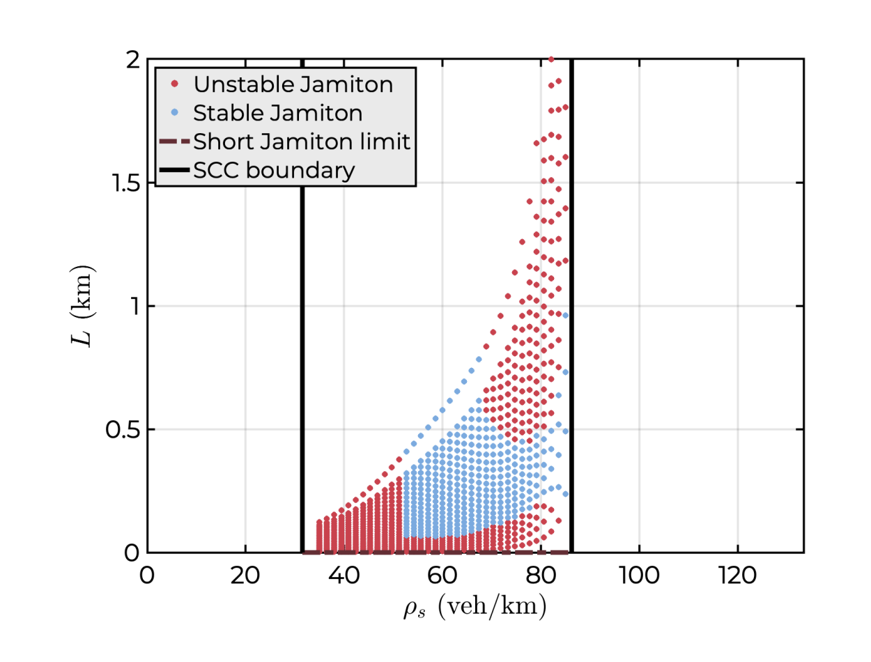
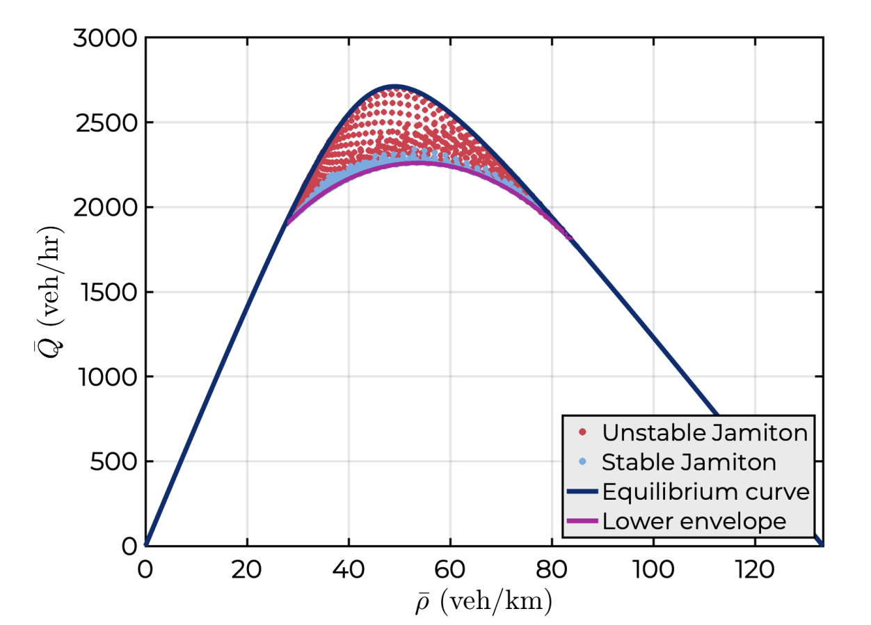
Figure 8. Stability plots obtained from [52] Left: Stable and unstable jamitons in the $(\rho_{s},L)$ plane. Right: Stable and unstable jamitons in the fundamental diagram.

In [52], the dynamical stability of jamitons under small perturbations was studied numerically. In this case, it was determined that stability depends on the size of the jamiton: very small jamitons are unstable because they collide with new jamitons arising from the perturbations, while larger jamitons are also unstable, but in this case, they split into two or more jamitons. Both cases are visible in the phase plane $(\rho_{s},L)$, as well as in the fundamental diagram, as shown in Figure 8. Additionally, in [58] both concepts of (orbital) stability and asymptotic stability of jamitons are also discussed. While the notion of stability is clearly obtained as the numerical survival of perturbations of jamitons (see also the previously cited work [52] for a deeper analysis), the notion of asymptotic stability is defined as the existence of exponentially decaying (in time) solutions for the corresponding linearized dynamics, also called sometimes in dispersive PDEs as “convective stability”. For further details, see [58, Chapter 5].

4. Simulation of the ARZ model

The numerical method for the discretization of the ARZ model (1.1) involves the well-known Harten-Lax-van Leer (HLL) [60] numerical flux, which represents an approximate Riemann solver. Since the ARZ model includes a relaxation term that makes it non-homogeneous, it is approximated by a two-step time-splitting scheme (cf.  [21, Chapter 17]): first, the homogeneous model is solved by using a finite volume scheme (involving the HLL numerical flux), and then, the differential equation

$$\partial_{t}\bm{Q}=\bm{S}(\bm{Q})$$ (4.1)

is solved, where $\bm{S}$ corresponds to the relaxation source term in the system. In each time step, the numerical solution of the ODE (4.1) is applied to the finite volume solution obtained in the previous step.

4.1. HLL solver for a system of conservation laws

A simple approximator that yields good results and ensures that the numerical flux satisfies the entropy condition [61] is the HLL numerical scheme [52]. To introduce the scheme, we consider the system of conservation laws

$$\partial_{t}\bm{Q}+\partial_{x}\bm{F}(\bm{Q})=\bm{0}$$ (4.2)

and assume a uniform grid of cells $I_{i,n}\coloneqq[x_{i-1/2},x_{i+1/2}]\times[t_{n},t_{n+1}]$, where it is assumed that $x_{i-1/2}=(i-1/2)\Delta x$ and $t_{n}=n\Delta t$ for $i\in\mathbb{Z}$ and $n\in\mathbb{N}_{0}$. If $\bm{Q}_{i}^{n}$ denotes an approximate value of the cell average of $\bm{Q}$ on $I_{i,n}$ then an explicit finite volume scheme for (4.2) can be written as the marching formula

$$\bm{Q}_{i}^{n+1}=\bm{Q}_{i}^{n}-(\Delta t/\Delta x)\bigl{(}\bm{\mathcal{F}}(\bm{Q}_{i}^{n},\bm{Q}_{i+1}^{n})-\bm{\mathcal{F}}(\bm{Q}_{i-1}^{n},\bm{Q}_{i}^{n})\bigr{)},$$ (4.3)

where $\bm{\mathcal{F}}=\bm{\mathcal{F}}(\bm{Q}_{L},\bm{Q}_{R})$ is a numerical flux function that among other properties should be consistent with the exact flux $\bm{F}=\bm{F}(\bm{Q})$ in the sense that $\bm{\mathcal{F}}(\bm{Q},\bm{Q})=\bm{F}(\bm{Q})$ for all $\bm{Q}$.

The HLL scheme is defined by the particular choice of $\bm{\mathcal{F}}=\bm{\mathcal{F}}(\bm{Q}_{L},\bm{Q}_{R})$ given by

$$\bm{\mathcal{F}}^{\mathrm{HLL}}(\bm{Q}_{L},\bm{Q}_{R})=\frac{1}{s_{R}^{+}-s_{L}^{-}}\bigl{(}s_{R}^{+}\bm{F}(\bm{Q}_{L})-s_{L}^{-}\bm{F}(\bm{Q}_{R})+s_{R}^{+}s_{L}^{-}(\bm{Q}_{R}-\bm{Q}_{L})\bigr{)},$$ (4.4)

where $s_{L}$ and $s_{R}$ are lower and upper estimates of the characteristic speeds involved in the solution of the Riemann problem for (4.2) defined for left and right states $\bm{Q}_{L}$ and $\bm{Q}_{R}$, and we define $a^{+}\coloneqq\max\{a,0\}$ and $a^{-}\coloneqq\min\{a,0\}$. For a hyperbolic system (4.2) of a general number $m$ of equations and unknowns, where the characteristic speeds (eigenvalues of the Jacobian matrix $\bm{J}_{\bm{F}}(\bm{Q})=(\partial F_{i}(\bm{Q})/\partial\phi_{j})_{1\leq i,j\leq m}$) are given by $\lambda_{1}(\bm{Q})\leq\lambda_{2}(\bm{Q})\leq\cdots\leq\lambda_{m}(\bm{Q})$, one may choose $s_{R}=\max\{\lambda_{m}(\bm{Q}_{L}),\lambda_{m}(\bm{Q}_{R})\}$ and $s_{L}=\min\{\lambda_{1}(\bm{Q}_{L}),\lambda_{1}(\bm{Q}_{R})\}$. These formulas are utilized for $m=2$ when (4.2) represents the the homogeneous version of the system of balance equations (2.15), and the corresponding characteristic speeds $\lambda_{1}$ and $\lambda_{2}$ are given by (2.12).

The preceding description is limited to the final form of the HLL scheme. For its motivation based on the simplified solution of the above-mentioned Riemann problem through a wave configuration that consists of just two waves separating three states (namely $\bm{Q}_{L}$, an intermediate one, and $\bm{Q}_{R}$) we refer to monographs on numerical schemes for conservation laws, for instance [22, 21, 23, 24].

4.2. Simulation with relaxation term

To incorporate the source term into the model, one simply needs to numerically solve the ODE (4.1), where the update accounts for the term $\bm{Q}_{i}^{*}$ obtained from simulating the homogeneous scheme. The non-homogeneous ARZ model written in conservative variables reads (2.15), where the source term $\bm{S}(\bm{Q})$ is given by the second equation of (2.14). Then one must solve (4.1) and since the relaxation term only appears in the second equation, it suffices to update the variable $y$. Equation (4.1) is solved using an implicit time-stepping scheme, as it is undesirable to impose additional CFL conditions on spatial and temporal steps, and to take advantage of the absence of a relaxation term for the variable $\rho$, simplifying the computational implementation. Discretizing (4.1) gives that

$$\frac{y_{i}^{n+1}-y_{i}^{*}}{\Delta t}=\frac{\rho_{i}^{n+1}U(\rho_{i}^{n+1})+h(\rho_{i}^{n+1})-y_{i}^{n+1}}{\tau},\qquad\rho_{i}^{n+1}=\rho_{i}^{*},$$ (4.5)

where the second equation holds because there is no source term for $\rho$. Thus, defining $\alpha\coloneqq\Delta t/\tau$, we obtain from (4.5) the following update scheme for the variable $y_{i}^{n+1}$:

$$y_{i}^{n+1}=\frac{\alpha}{\alpha+1}(\rho_{i}^{*}U(\rho_{i}^{*})+h(\rho_{i}^{*}))+\frac{1}{\alpha+1}y_{i}^{*},$$

where $\rho_{i}^{*}$ and $y_{i}^{*}$ are obtained from (4.3) with $\bm{Q}_{i}^{n+1}$ replaced by $\bm{Q}_{i}^{*}=(\rho_{i}^{*},y_{i}^{*})^{\mathrm{T}}$.

4.3. Results

In [62], several simulations of traffic jams on circular roads and the appearance of initially small jamitons, also known as “jamitinos,” on an infinite road are presented. To validate the scheme, the results obtained in [62] will be emulated, and error tables between the simulation with a jamiton as the initial condition and its theoretical solution will also be presented. In all simulations, periodic boundary conditions (circular road) were considered. The benefit of this type of conditions is the preservation of vehicular mass over time since there are no exits or entrances of vehicles, meaning that the number of vehicles $N$ given by

$$N(t)\coloneqq\int_{0}^{L}\rho(x,t)\,\mathrm{d}x,$$

is constant for all times $t$. This provides another way to validate the numerical simulations.

4.4. Example 1: accuracy of the numerical scheme

(a)	(b)
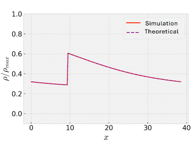
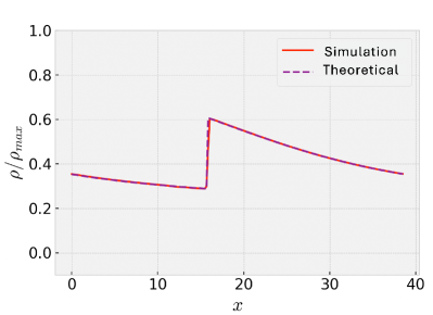
(c)	(d)

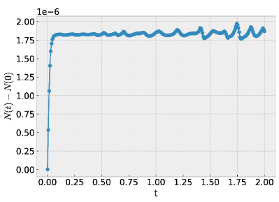
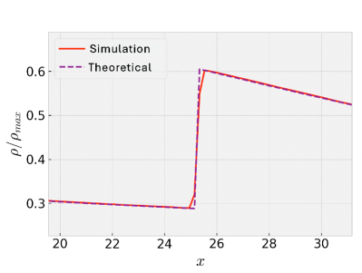
Figure 9. Example 1 (accuracy test): sample comparison between the numerical simulation and theoretical jamiton with $\rho_{s}=0.433\rho_{\max}$, $v_{-}=26$, and $\mathcal{N}=200$: (a) jamiton-like initial condition, (b) comparison of exact and numerical solutions at simulated time $t=1.01$, (c) numerically simulated number of vehicles (for the exact solution, the difference $N(t)-N(0)$ should be zero), (d) enlarged view of the exact and numerical solutions at simulated time $t=2.47$.

Table 1. Example 1 (accuracy test): errors for various values of $\mathcal{N}$, $\tau$, and simulated times $t_{\mathrm{final}}$.

	$t_{\mathrm{final}}=0.5$						$t_{\mathrm{final}}=2$
	$\tau=1$		$\tau=5$		$\tau=10$		$\tau=1$		$\tau=5$		$\tau=10$
$\mathcal{N}$	$\varepsilon_{\rho}^{\Delta x}$	$\varepsilon_{u}^{\Delta x}$	$\varepsilon_{\rho}^{\Delta x}$	$\varepsilon_{u}^{\Delta x}$	$\varepsilon_{\rho}^{\Delta x}$	$\varepsilon_{u}^{\Delta x}$	$\varepsilon_{\rho}^{\Delta x}$	$\varepsilon_{u}^{\Delta x}$	$\varepsilon_{\rho}^{\Delta x}$	$\varepsilon_{u}^{\Delta x}$	$\varepsilon_{\rho}^{\Delta x}$	$\varepsilon_{u}^{\Delta x}$
20	5.908	2.661	2.519	1.205	1.779	0.862	19.760	9.725	6.055	2.690	3.524	1.663
40	3.079	1.445	1.992	0.874	1.187	0.526	11.521	5.495	2.837	1.251	2.589	1.226
80	1.437	0.667	0.594	0.296	0.957	0.402	7.052	3.282	1.308	0.622	1.092	0.491
160	1.028	0.503	0.350	0.170	0.290	0.143	4.473	2.021	0.722	0.363	0.493	0.246
320	0.649	0.304	0.203	0.111	0.179	0.088	2.834	1.235	0.337	0.187	0.217	0.127
640	0.244	0.123	0.103	0.051	0.131	0.072	1.207	0.538	0.186	0.106	0.140	0.088
1280	0.099	0.048	0.070	0.034	0.086	0.046	0.487	0.235	0.094	0.064	0.120	0.067
2560	0.055	0.026	0.050	0.025	0.073	0.039	0.295	0.144	0.065	0.044	0.094	0.053

The scheme described in Section 4.2 was applied to an initial jamiton-like solution constructed in Section 3. The simulation was run until a final time $t_{\mathrm{final}}$ and compared with the theoretical (exact) solution given by $\bm{Q}_{\mathrm{theo}}(x,t)\coloneqq\bm{Q}_{\mathrm{jam}}((x-st)/\tau)$, where $\bm{Q}_{\mathrm{jam}}$ is obtained from the construction in Section 3.3. The relative $L^{1}$ error

$$\varepsilon^{\Delta x}\coloneqq 100\frac{\|\bm{Q}_{\Delta x}-\bm{Q}_{\mathrm{theo}}\|_{L^{1}}}{\|\bm{Q}_{\mathrm{theo}}\|_{L^{1}}}$$

of a numerical solution $\bm{Q}_{\Delta x}$ computed with a spatial discretization $\Delta x$ was calculated for various grid refinements and values of the relaxation parameter $\tau$. See Figure 9 for further details.

In Table 1, the errors obtained for $t_{\mathrm{final}}=0.5$ and $t_{\mathrm{final}}=2$, respectively, for three different values of $\tau$ are shown. These errors correspond to a fixed jamiton with $\rho_{s}=0.433\rho_{\max}$ and $v_{-}=26$. As expected, as the mesh becomes finer, the solution better approximates the theoretical solution. However, for $\tau=1$, the errors are larger for both final times compared to $\tau=5$ and $\tau=10$. This could indicate that the simulation does not accurately approximate the exact solution when $\tau$ is small, especially if one wishes to study the convergence of ARZ to LWR as $\tau$ tends to 0. This case will not be covered in this work, but in [21, Chap. 17], an approach and a fractional step update for $\tau\to 0$ are proposed.

4.5. Example 2: emergence of jamitons

(a)	(b)
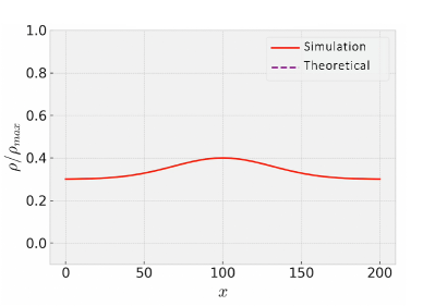
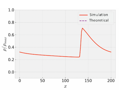
(c)	(d)

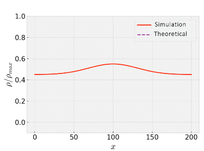
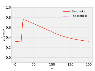
Figure 10. Example 2 (emergence of jamitons): examples with (a, b) low initial density, (c, d) high initial density; (a, c) initial condition, (b, d) formation of a jamiton at simulated time (b) $t=13.42$, (d) $t=23.07$.

In Figure 10 formations of jamitons are observed with initial conditions that emulate a small perturbation. The size and displacement of the obtained jamitons depend to some extent on the initial density, which in all cases was chosen to violate the SCC. In the case of Figures 10(a) and (b), the jamiton travels with positive velocity to the right, while in Figures 10(c) and (d), the resulting jamiton, besides being longer, moves with negative velocity, i.e., towards the left.

4.6. Example 3: jamitons on a long circular road

(a)	(b)

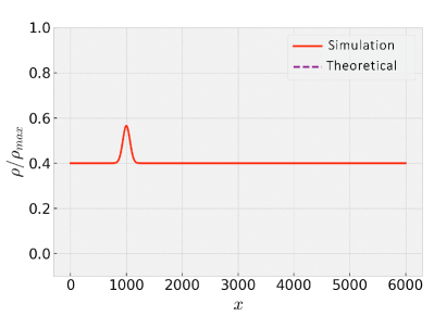
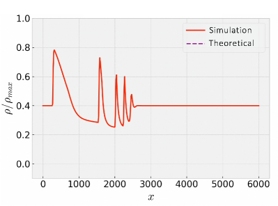
(c)

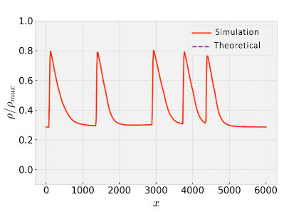
Figure 11. Example 3 (jamitons on a long circular road): (a) initial condition, (b) formation of a large jamiton and several jamitinos at $t=117.09$, (c) solution is governed by the jamitonic regime at $t=1646.79$.

In Figure 11, the formation of so-called “jamitinos”, i.e., initially small jamitons, as shown in [62], is observed. The setting is as follows: one starts from a more pronounced Gaussian initial condition on a circular road six kilometers long, essentially approximating an infinite road. After some time, a chain of jamitinos with positive velocity forms from a larger jamiton with negative velocity. Since one is modeling a circular road, naturally the large jamiton collides with some jamitinos. What is observed is that the result of colliding two jamitons is another jamiton, but with different length and velocity compared to those initiated before the collision. This will be examined in more detail in Section 5. In Figure 11(c), the simulation of jamitons was run for a long time. It is observed that the solution is dominated by a jamitonic regime, with several jamitons connected by jumps and of equal amplitude but apparently of different lengths. This situation can occur if each jamiton has a different sonic density $\rho_{s}$. It can also be noted that all jamitons in Figure 11(c), being connected by jumps, share the parameter $\rho_{-}$. This observation will be important for establishing the collision scheme in Section 5.

4.7. Example 4: approximation of the jamiton propagation velocity

Table 2. Example 4 (approximation of the jamiton propagation velocity): errors in $s$ and $m$ for various values of $\mathcal{N}$ and $\tau$ at simulated times $t_{\mathrm{final}}=2$.

	$\tau=1$		$\tau=5$		$\tau=10$
$\mathcal{N}$	$\varepsilon^{\Delta x}_{s}$	$\varepsilon^{\Delta x}_{m}$	$\varepsilon^{\Delta x}_{s}$	$\varepsilon^{\Delta x}_{m}$	$\varepsilon^{\Delta x}_{s}$	$\varepsilon^{\Delta x}_{m}$
20	0.01623	0.03049	0.00371	0.01826	0.03326	0.02255
40	0.00312	0.01316	0.00522	0.00253	0.01849	0.01286
80	0.00410	0.00235	0.00566	0.00125	0.01087	0.00785
160	0.00429	0.00007	0.00526	0.00272	0.00701	0.00533
320	0.00423	0.00128	0.00487	0.00328	0.00473	0.00374
640	0.00171	0.00048	0.00248	0.00170	0.00209	0.00162
1280	0.00029	0.00008	0.00233	0.00179	0.00091	0.00070
2560	0.00025	0.00006	0.00165	0.00131	0.00063	0.00051

An important value to obtain from the simulation of jamitons is the propagation velocity, especially if one wishes to study numerically jamitons and the theoretical parameters of the jamiton are unknown. A first approximation would be to obtain $\rho_{+}$ and $\rho_{-}$ from the simulation, since $\rho_{+}$ and $\rho_{+}$ are the maximum and minimum of $\rho(x,t)$ for a jamiton-like solution at arbitrary, sufficiently large time $t$ (i.e., when the solution has attained the traveling wave regime). With these parameters, the value of $\rho_{s}$ can be approximated using the construction of a jamiton. However, this method has a high error rate since it depends only on two points of the simulation, and the error of the numerical scheme could propagate in the estimation of $\rho_{s}$. Therefore, another way to approximate $s$ and $m$ that has higher precision is desirable. In Section 3 we demonstrated that jamitons corresponded to line segments in the fundamental diagram, and that these line segments intersect the equilibrium curve at $(\rho_{s},Q(\rho_{s}))$, where $m$ and $s$ correspond to the intersection and slope of the line passing through the segment, respectively. This result allows us to approximate the velocity of propagation of a jamiton by resorting to the $(\rho,q)$ plane. The method for obtaining this was presented in [52]. It consists in taking a jamiton-like solution obtained from the simulation $\rho_{\mathrm{jam}}$ and $u_{\mathrm{jam}}$, and plotting the obtained data in the $(\rho,q)$ plane (i.e., plotting $(\rho_{\mathrm{jam}},\rho_{\mathrm{jam}}u_{\mathrm{jam}})$). The expected result would correspond to a line segment with the parameters of the jamiton. Thus, $m_{\mathrm{jam}}$ and $s_{\mathrm{jam}}$ can be obtained from a linear regression of the mentioned plot.

To observe the effectiveness of the method, a jamiton with $\rho_{s}=0.433\rho_{\max}$ and $v_{-}=26$ was taken as the initial condition (as in Example 1). The relative error between $s$ and $m$ of the jamiton and the one obtained by linear regression was calculated, given by:

$$\varepsilon^{\Delta x}_{s}=100\frac{|s_{\Delta x}-s_{\mathrm{theo}}|}{|s_{\mathrm{theo}}|},\qquad\varepsilon^{\Delta x}_{m}=100\frac{|m_{\Delta x}-m_{\mathrm{theo}}|}{|m_{\mathrm{theo}}|}.$$

For this particular jamiton, we have $m_{\mathrm{theo}}\approx 0.356$ and $s_{\mathrm{theo}}\approx 6.374$. The effectiveness of the method was tested by running the simulation until $t_{\mathrm{final}}=2$ for $\tau=1,5,10$ with increasingly finer grids. The results are shown in Table 2. The effectiveness of the method is evident from Table 2, even with relatively coarse grids, and its precision increases as the grid becomes finer. This method will be used in Section 5 to determine the exit velocities of the jamitons resulting from the collision of jamitons.

5. Collision of jamitons

5.1. Compatibility of jamitons

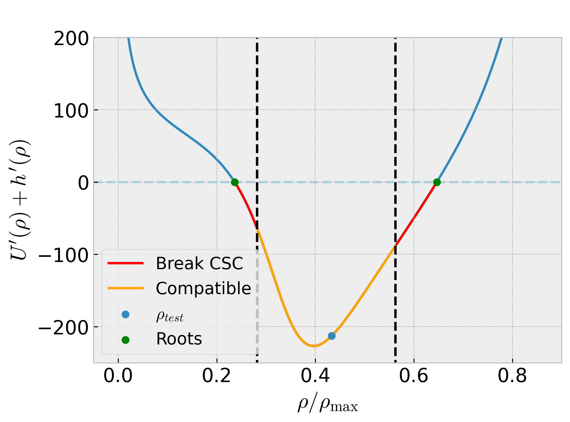
Figure 12. Compatible densities with a test jamiton. In red, possible densities that break the SCC condition.

As mentioned in Section 4, the collision of jamitons was observed in the formation of jamitinos on a circular route. In such a case, the collision of two jamitons results in a new jamiton with parameters possibly different from those of the original jamitons. Additionally, it was observed that for two jamitons to collide, they must share the value of $\rho_{-}$, as they necessarily must be connected by the jump between $\rho_{-}$ and $\rho_{+}$ (or in Lagrangian variables, between $v_{+}$ and $v_{-}$). Indeed, consider two jamiton-type solutions $\smash{Q_{\mathrm{jam}}^{1}}$ and $\smash{Q_{\mathrm{jam}}^{2}}$ with parameters $\rho_{s}^{1}$, $v_{-}^{1}$, $v_{+}^{1}$, and and $\rho_{s}^{2}$, $v_{-}^{2}$, and $v_{+}^{2}$, respectively. The idea is to obtain a necessary condition for $\smash{Q_{\mathrm{jam}}^{1}}$ to be able to join $\smash{Q_{\mathrm{jam}}^{2}}$. The smooth part of $\smash{Q_{\mathrm{jam}}^{1}}$ is obtained by integrating the ODE (3.5) between $v_{+}^{1}$ and $v_{-}^{1}$. However, “the jump of $\smash{Q_{\mathrm{jam}}^{2}}$” connects the values $v_{-}^{2}$ with $v_{+}^{2}$, so if one wants to join the smooth part of $\smash{Q_{\mathrm{jam}}^{1}}$ with “the jump of $\smash{Q_{\mathrm{jam}}^{2}}$,” necessarily $v_{-}^{1}=v_{-}^{2}$. This condition will be known as the compatibility condition between jamitons.

Definition 5.1 (Compatibility).

Two jamitons $\smash{Q_{\mathrm{jam}}^{1}}$ and $\smash{Q_{\mathrm{jam}}^{2}}$ with parameters $v_{-}^{1}$ y $v_{-}^{2}$, respectively, will be compatible if $v_{-}^{1}=v_{-}^{2}$.

It can be noted that the compatibility condition does not completely restrict the values of $\rho_{s}$ or $v_{+}$, even though the latter depends on both $\rho_{s}$ (since $m=m(\rho_{s})$ and $s=s(\rho_{s})$) and $v_{-}$. Since the family of jamiton solutions is parametrized by $\rho_{s}$, it is possible to study the compatibility of various jamitons of different sizes and lengths based on their sonic density for a fixed jamiton given by $\rho_{s}$. First, a $\rho_{\mathrm{test}}$ will be chosen such that the selection interval for $v_{-}$ is the largest among the densities that break the SCC, and $v_{-}^{\mathrm{test}}$ will be chosen as the midpoint of the interval found. Then, sonic densities will be chosen such that the maximal jamiton interval given by $[v_{R},v_{M}]$ contains $v_{-}^{\mathrm{test}}$. The densities found are shown in Figure 12. The test jamiton chosen has parameters $\rho_{s}\approx 0.4333$ and $v_{-}^{\mathrm{test}}\approx 26.602$.

This ensures that the study of collisions considers a variable amount of different sizes and lengths, and that the jamitons to collide are compatible, as $v_{-}^{\mathrm{test}}$ can be chosen within the jamitons to collide. However, the first step of choosing $\rho_{s}^{\mathrm{test}}$ can be done for any $\rho_{s}$ that breaks the SCC. The particular choice made was to maximize the number of possible collisions with a single test jamiton.

5.2. Example 5: collision between two compatible jamitons

(a)

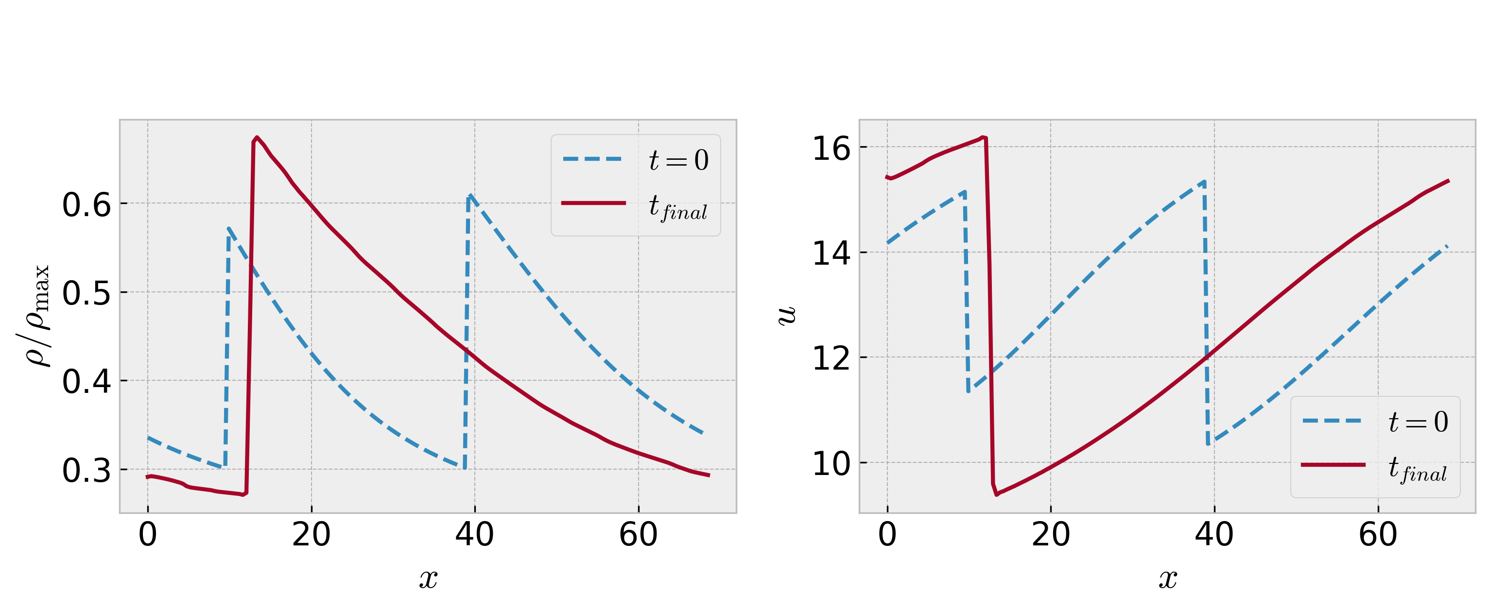
(b) (c)

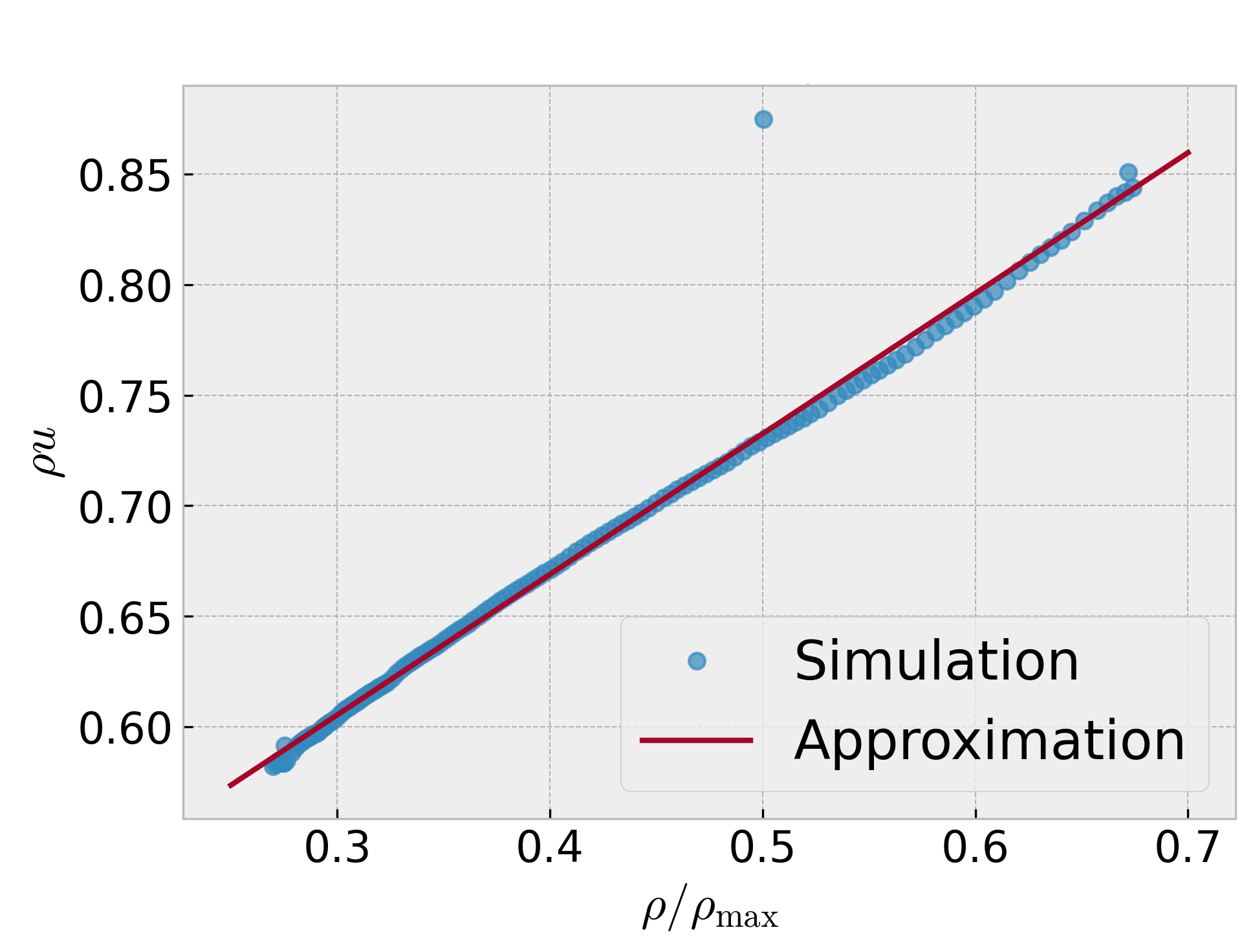
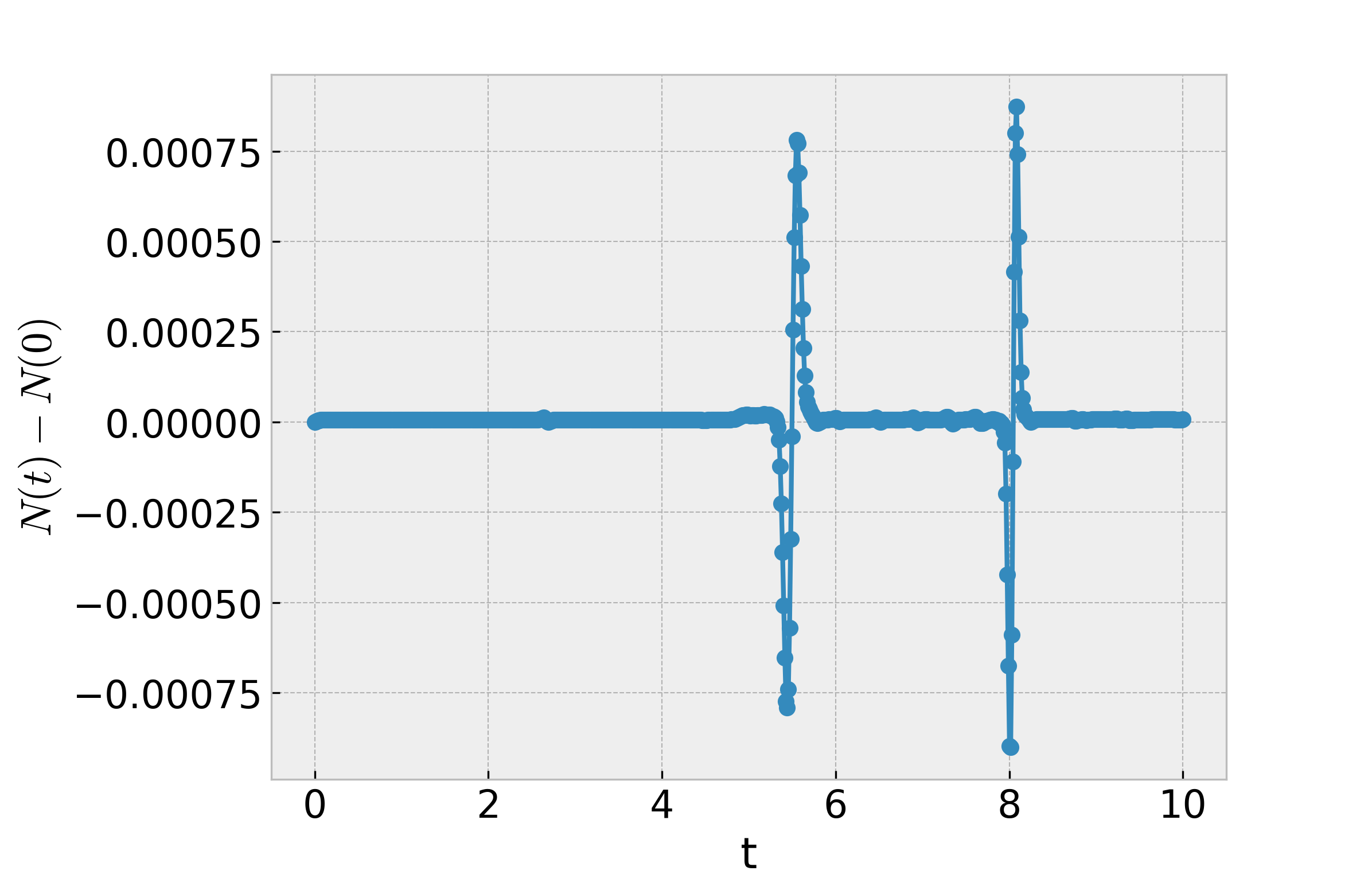
Figure 13. Example 5 (collision between two compatible jamitons): (a) collision between a jamiton with $\rho_{s}=0.425\rho_{\max}$ and another with $\rho_{s}=0.443\rho_{\max}$, both with $v_{-}=25$ shown in the variables (left) $\rho$ and (right) $u$, (b) segment in the $(\rho,q)$-plane approximating the jamiton obtained from the collision in (a) (supporting the appearace of a post-collision jamiton), (c) illustration that the collision algorithm maintains the conservation law with little variation in the total number of vehicles.

As mentioned in Section 4, in the simulation of jamitinos, various collisions between jamitinos with different velocities are observed, as well as some being absorbed by the larger initial jamiton. This leads to the following conjecture, whose validation at the moment is purely numerical and can be observed in Figure 13.

Conjecture 5.2.

The collision of two compatible jamitons generates a unique new jamiton whose parameters depend on the original jamitons.

This conjecture is crucial as the simulations are conducted with the anticipation of the emergence of a new jamiton. The selected jamitons are merged with the test jamiton, which is then imposed as the initial condition in the simulation. The code is then allowed to run until a sufficiently long time has elapsed for the resulting jamiton from the collision to form. Since this jamiton is obtained purely numerically, to obtain its properties, such as $m$ and $s$, the method described in Section 4.7 is used based on the behavior of a jamiton in the fundamental diagram. Figure 13(a) shows an example of how two jamitons collide and the resulting jamiton after a time $t_{\mathrm{final}}$. In Figure 13(b), the segment approximating the post-collision jamiton in the $(\rho,q)$ plane is observed.

5.3. Example 6: simulation of multiple collisions

(a)	(b)
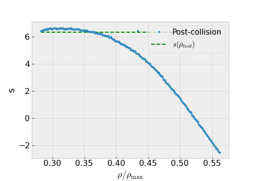
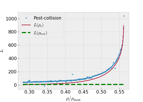
(c)	(d)

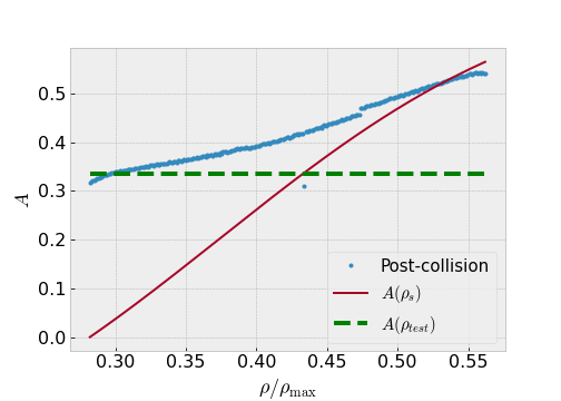
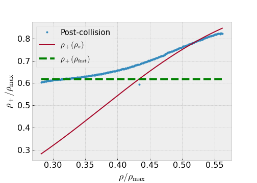
(e)

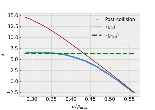
Figure 14. Example 6 (simulation of multiple collisions): (a) plot of post-collision exit velocities (the data at $\rho/\rho_{\max}\approx 0.44$ corresponds to jamitons that did not collide because they had very close values of $\rho_{s}$; note the small initial bump that appears in the post-collision exit velocities), (b) lengths obtained after each collision, (c) amplitudes obtained after each collision, (d) values of $\rho_{+}$ after each collision, (e) comparison with function $s(\rho_{s})$.

With the proposed algorithm, 274 different collisions are performed between the test jamiton and the compatible jamitons, where we use $\tau=5$ and $\mathcal{N}=160$ as the total number of points in the grid, and $\Delta t$ such that the CFL condition $s_{\max}\Delta t/\Delta x\leq 1/2$ is satisfied. The simulations of the various collisions were run in parallel on 20 HPC clusters. The resulting jamitons from the collisions have their propagation velocities calculated, as seen in Figure 14(a) as a function of the densities $\rho_{s}$ compatible with the test jamiton. Other properties can be calculated from the post-collision jamitons, such as length and amplitude given by equations (3.8) and (3.10).

Figures 14(b) and (c) show the lengths and amplitudes of the resulting jamitons as a function of the compatible $\rho_{s}$ values and compared to those of the jamitons before colliding. The dashed line represents the test jamiton. Figure 14(d) presents the values of $\rho_{+}$ after each collision. Similarly, the exit velocities can be compared along with the function $s(\rho_{s})$, resulting in the graph in Figure 14(e).

An interesting result can be observed in Figure 14(a) for $\rho_{s}/\rho_{\max}\in[0.26,0.35]$. Note that for some collisions, the exit velocities increased compared to the test jamiton. This could indicate that a jamiton can accelerate if it collides with smaller-sized jamitons, and if the relationship between velocity and size meets certain properties, it could even decrease the size of a jamiton. This provides an important tool in practical applications, as traffic could potentially be disentangled by colliding with chains of smaller-sized jamitons. On the other hand, in Figure 14(e) it can be observed that the exit velocities correspond to a smoothing between the constant $\rho_{\mathrm{test}}$ and the function $s(\rho_{s})$. This indicates that the predominant jamitons after the collision are those of larger size, meaning that the smaller jamitons in length and amplitude are absorbed by the larger ones. However, in the collisions of jamitons with $\rho_{s}/\rho_{\max}\in[0.40,0.45]$, there is a certain additivity in their amplitudes, as the amplitude obtained after the collision turns out to be greater than the amplitudes before the collision. A contrary effect, observable in Figure 14(e), occurs with the exit velocities, which decrease compared to the input jamitons for the same density range. This phenomenon can be summarized in the following conjecture:

Conjecture 5.3 (Post-collision inequalities).

Let $Q_{\mathrm{jam}}$ be a jamiton with sonic density $\rho_{s}$. Let $\smash{\{Q_{\mathrm{jam}}(\rho_{s}^{\mathrm{jam}})\}}$ be a corresponding non-empty set of compatible jamitons parametrized by their sonic densities $\rho_{s}^{\mathrm{jam}}$. Let $Q_{\mathrm{post}}$ be the jamiton obtained from the collision of $Q_{\mathrm{jam}}$ with $\smash{Q_{\mathrm{jam}}(\rho_{s}^{\mathrm{jam}})}$ and with sonic density $\rho_{s}^{\mathrm{post}}$. Then the following hold:

• There exists a $\rho_{s}^{0}$ such that $\smash{s(\rho_{s}^{\mathrm{post}})\leq s(\rho_{s})}$ for all $\rho_{s}^{\mathrm{jam}}\geq\rho_{s}^{0}$ and $s(\rho_{s}^{\mathrm{post}})\leq s(\rho_{s}^{\mathrm{jam}})$ for all $\rho_{s}^{\mathrm{jam}}$.

• There exists a $\rho_{s}^{1}$ such that $A(\rho_{s}^{\mathrm{post}})\geq A(\rho_{s}^{\mathrm{jam}})$ for all $\rho_{s}^{\mathrm{jam}}\leq\rho_{s}^{1}$.

• $L(\rho_{s}^{\mathrm{post}})\geq L(\rho_{s})$ and $L(\rho_{s}^{\mathrm{post}})\geq L(\rho_{s}^{\mathrm{jam}})$ for all $\rho_{s}^{\mathrm{jam}}$.

5.4. Example 7: effect of the relaxation time

(a)	(b)
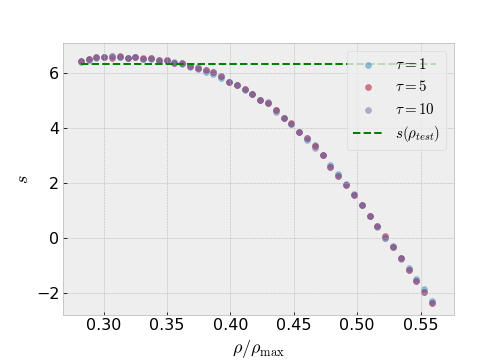
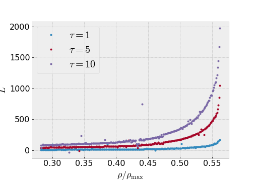
(c)	(d)

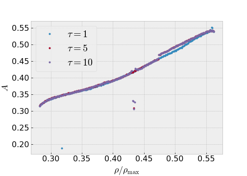
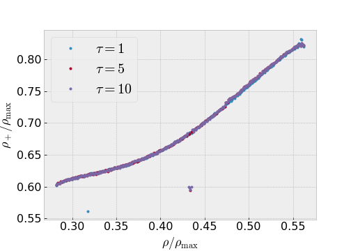
Figure 15. Example 7 (effect of the relaxation time): (a) plot of post-collision exit velocities , (b) lengths and (c) amplitudes of the resulting jamiton, (d) values of $\rho_{+}$, all for various values of $\tau$.

(a)	(b)

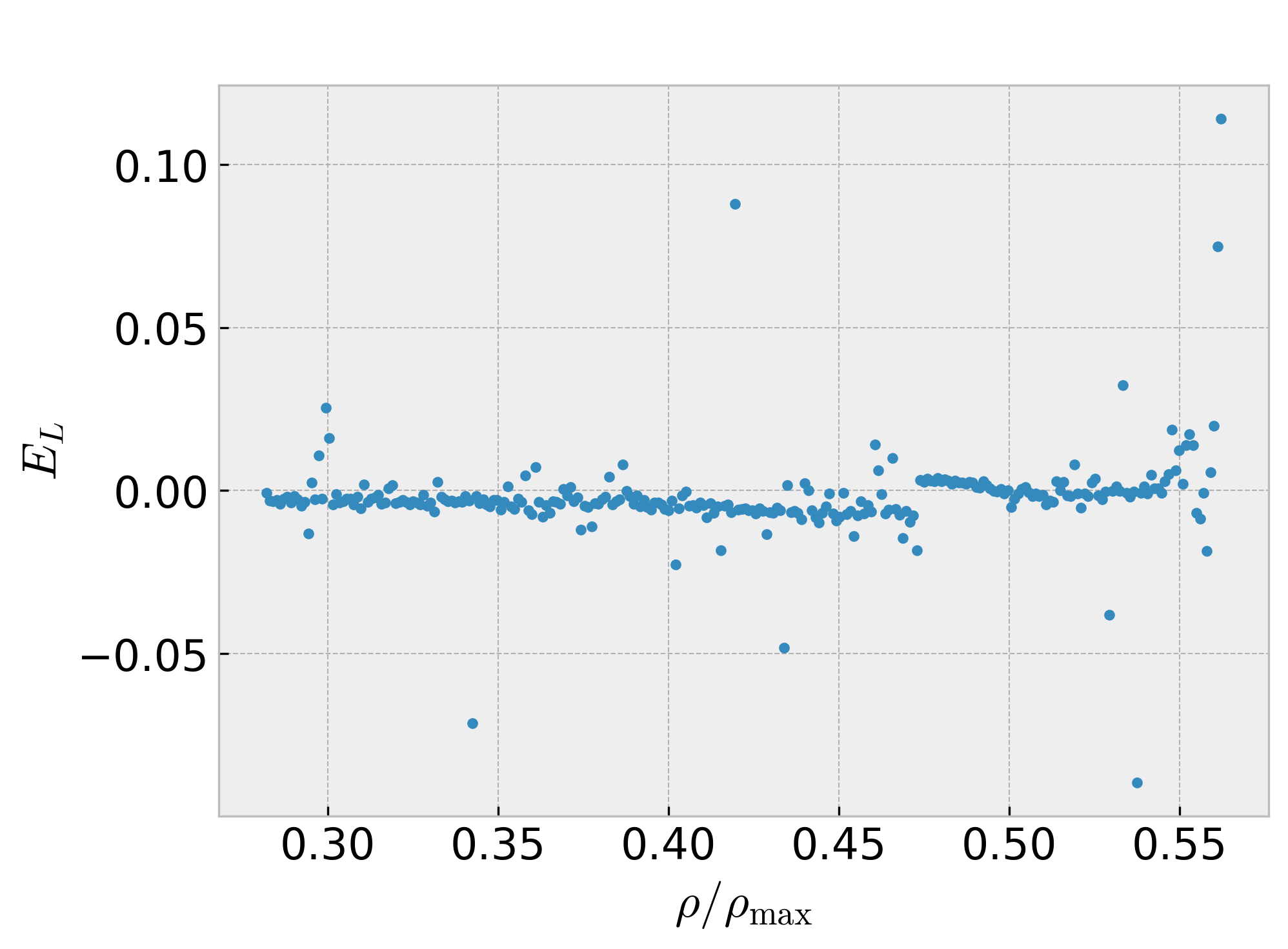
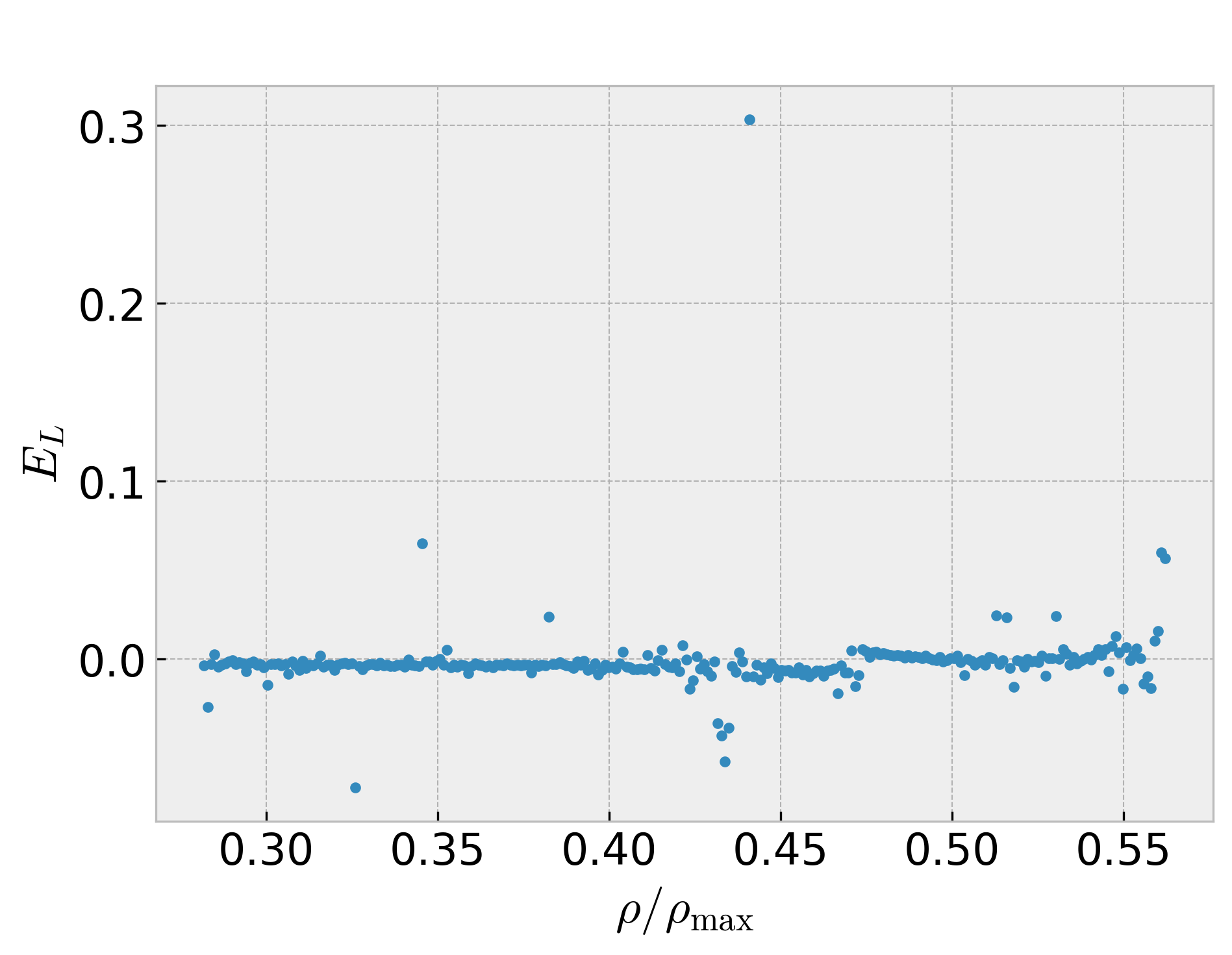
(c)

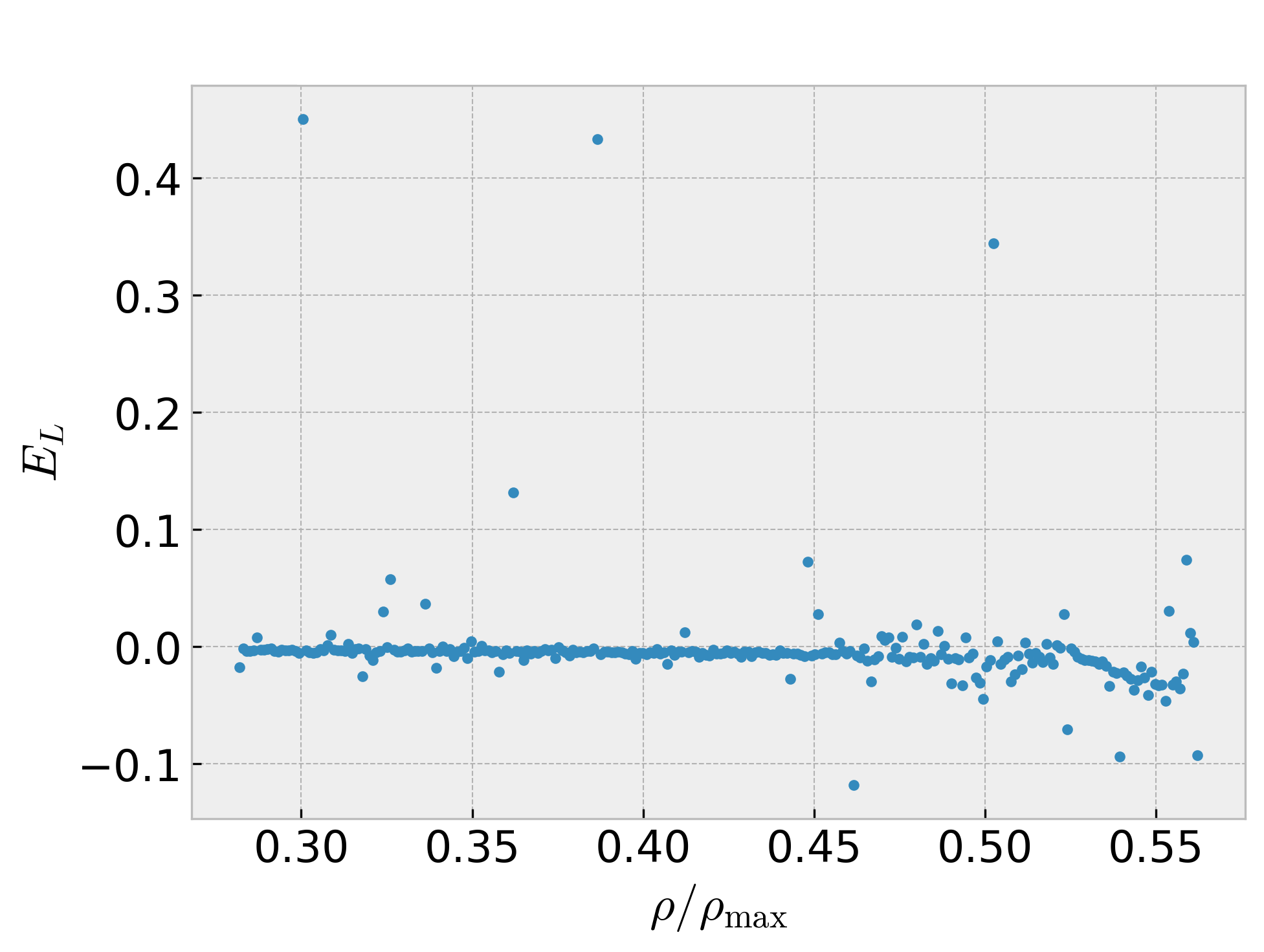
Figure 16. Example 7 (effect of the relaxation time): normalized length error $E_{L}$ for (a) $\tau=5$, (b) $\tau=10$ and (c) $\tau=1$.

An interesting question is whether the same phenomenon persists for different values of the relaxation time $\tau$, where we recall that this parameter appears recurrently in the theoretical study of jamitons. To answer this question, the same experiment conducted previously is repeated, but with two additional different values of $\tau$ ($\tau=1$ and $\tau=10$). The outcome of the collisions is observed in Figure 15(a). The behavior of the exit velocities is consistent across different values of $\tau$. This makes sense because both $m$ and $s$ depend only on the sonic density, not on the value of $\tau$. This leads to the following conjecture:

Conjecture 5.4.

The sonic velocity of the jamiton resulting from a collision is independent of $\tau$.

The other properties of a jamiton, such as the amplitude, length, and $\rho_{+}$, can also be studied by varying $\tau$. In Figures 15(b) to (d), the amplitudes, lengths, and $\rho_{+}$ for $\tau=1$, $5$, and $10$ are obtained. It can be observed that such properties also do not depend on $\tau$. This is also expected because both $\rho_{+}$ and $\rho_{-}$ depend only on $\rho_{s}$, which in turn is independent of $\tau$. This adds more invariants to the collision of jamitons:

Conjecture 5.5.

The amplitude and value of $\rho_{+}$ of the jamiton resulting from a collision are independent of $\tau$.

However, in Figure 15(b), it is observed that the length of the post-collision jamiton changes, being greater as $\tau$ increases. This effect is related to the formula for length given in (3.8), which depends on $\tau$. This leads to the following conjecture:

Conjecture 5.6.

The length of the jamiton resulting from a collision depends on $\tau$.

It is interesting to study whether there is additivity in the lengths of the jamitons, that is, whether the length of the jamiton post-collision corresponds to the sum of the lengths of the jamitons before colliding. For this, the lengths of the jamitons before collision are calculated, summed up, and compared to the lengths post-collision. The following normalized error is defined:

$$E_{L}\coloneqq\frac{L_{\text{col}}-(L+L_{\mathrm{test}})}{\displaystyle\max_{\rho}{\left(L+L_{\mathrm{test}}\right)}},$$ (5.1)

where $L_{\text{col}}$ corresponds to the length of the jamiton post-collision, $L_{\mathrm{test}}$ to the length of the test jamiton, and $L$ to the length of the jamiton collided with the test jamiton. Figure 16 shows the results obtained for $E_{L}$ in (5.1). It is observed that indeed the error is small, especially for the case $\tau=5$. Additionally, the most noticeable differences could perfectly be caused by numerical errors in the simulation. This leads to the following conjecture:

Conjecture 5.7.

The length of the jamiton after colliding corresponds to the sum of the lengths of the colliding jamitons.

6. Conclusions

To conclude this work, a summary of the content and results in each section is provided, along with potential future lines of development. Section 2 introduced properties of the most used traffic models, being the inhomogeneous ARZ one of the key models studied here. In Section 3, the theoretical derivation of jamitons and their properties was observed. In Section 4, the numerical scheme was validated under numerical errors and comparisons with theoretical jamitons. Finally, in Section 5, several results in the collision of jamitons were defined and numerically tested: the collision of jamitons originates a new jamiton, the exit velocities correspond to the smoothing of two functions, the exit lengths increase, as well as the amplitudes (in a density range), and properties dependent and independent of $\tau$ post-collision were observed..

The collision of jamitons leaves several open questions to be answered, especially in the theoretical realm, as the results of this paper are only numerical but can provide direction for eventual proofs. Therefore, theoretical explanations or mathematically robust validations are tasks for future work. On the other hand, further experimentation with numerical simulations can be carried out to explore beyond double collisions. For example, simulating triple, quadruple collisions, or even collisions of $N$ jamitons. Of course, the results at this point must be carefully analyzed as they correspond to cases of greater complexity and whose final outcome is highly non-trivial. Similar cases have been studied in other types of systems, such as the Schrödinger equation where there is an explicit solution for the interaction of $N$ solitons [63]. Following this line, one can also experiment with ’bombardments’ using chains of jamitons on a larger-sized jamiton, hoping to decrease its amplitude and, in simpler terms, alleviate traffic congestion. The veracity of this effect is unknown, but Figure 14 suggests that at least the speed of the larger jamiton can be increased.

Another experiment that can be carried out is to collide using other functions $h$, $U$, or $Q$ determined from another more localized fundamental diagram. For example, specific routes in a city or country. In this way, numerical simulations can be adjusted to different realities, as well as being able to apply them in real life and solve everyday problems.

Finally, a future work that can be carried out, although it deviates slightly from the theme of the paper, is to implement control models for traffic jams through numerical simulations of jamitons. As mentioned earlier, empirical control experiments have been conducted, but there is no mathematical rigor regarding them, so a good future work would be to experiment with these cases under numerical simulations and derive theoretical results.

References

- [2] Flynn, M. R., Kasimov, A. R., Nave, J.-C., Rosales, R. R., and Seibold, B., “Self-sustained nonlinear waves in traffic flow”, Phys. Rev. E (3), vol. 79, no. 5, pp. 056113, 13, 2009, doi:10.1103/PhysRevE.79.056113.
- [3] Seibold, B., Flynn, M. R., Kasimov, A. R., and Rosales, R. R., “Constructing set-valued fundamental diagrams from jamiton solutions in second order traffic models”, Netw. Heterog. Media, vol. 8, no. 3, pp. 745–772, 2013, doi:10.3934/nhm.2013.8.745.
- [4] Garavello, M., Han, K., and Piccoli, B., Models for vehicular traffic on networks, vol. 9 de AIMS Series on Applied Mathematics. American Institute of Mathematical Sciences (AIMS), Springfield, MO, 2016.
- [5] Treiber, M. and Kesting, A., Traffic flow dynamics. Springer, Heidelberg, 2013, doi:10.1007/978-3-642-32460-4. Data, models and simulation, Translated by Treiber and Christian Thiemann.
- [6] Aw, A. and Rascle, M., “Resurrection of “second order” models of traffic flow”, SIAM J. Appl. Math., vol. 60, no. 3, pp. 916–938, 2000, doi:10.1137/S0036139997332099.
- [7] Zhang, H. M., “A non-equilibrium traffic model devoid of gas-like behavior”, Transp. Res. Part B, vol. 36, pp. 275–290, 2002, doi:10.1016/S0191-2615(00)00050-3.
- [8] Nagel, K. and Schreckenberg, M., “A cellular automaton model for freeway traffic”, Journal de Physique I, vol. 2, p. 2221, 1992, doi:10.1051/jp1:1992277.
- [9] Lighthill, M. J. and Whitham, G. B., “On kinematic waves. II. A theory of traffic flow on long crowded roads”, Proc. Roy. Soc. London Ser. A, vol. 229, pp. 317–345, 1955, doi:10.1098/rspa.1955.0089.
- [10] Richards, P. I., “Shock waves on the highway”, Operations Res., vol. 4, pp. 42–51, 1956, doi:10.1287/opre.4.1.42.
- [11] Hilliges, M. and Weidlich, W., “A phenomenological model for dynamic traffic flow in networks”, Transp. Res. Part B, vol. 29, pp. 407–431, 1995, doi:10.1016/0191-2615(95)00018-9.
- [12] Bürger, R., García, A., Karlsen, K. H., and Towers, J. D., “A family of numerical schemes for kinematic flows with discontinuous flux”, J. Engrg. Math., vol. 60, no. 3-4, pp. 387–425, 2008, doi:10.1007/s10665-007-9148-4.
- [13] Bürger, R., Contreras, H. D., and Villada, L. M., “A Hilliges-Weidlich-type scheme for a one-dimensional scalar conservation law with nonlocal flux”, Netw. Heterog. Media, vol. 18, no. 2, pp. 664–693, 2023, doi:10.3934/nhm.2023029.
- [14] Jin, W.-L., Introduction to network traffic flow theory. Elsevier, Amsterdam, 2021, doi:10.1016/C2017-0-03540-1. Principles, concepts, models, and methods.
- [15] Aw, A., Klar, A., Materne, T., and Rascle, M., “Derivation of continuum traffic flow models from microscopic follow-the-leader models”, SIAM J. Appl. Math., vol. 63, no. 1, pp. 259–278, 2002, doi:10.1137/S0036139900380955.
- [16] Alperovich, T. and Sopasakis, A., “Stochastic description of traffic flow”, J. Stat. Phys., vol. 133, no. 6, pp. 1083–1105, 2008, doi:10.1007/s10955-008-9652-6.
- [17] Work, D., Tossavainen, O.-P., Blandin, S., Bayen, A., Iwuchukwu, T., and Tracton, K., “An Ensemble Kalman Filtering approach to highway traffic estimation using GPS enabled mobile devices”, Proceedings of the IEEE Conference on Decision and Control, pp. 5062–5068, 2008, doi:10.1109/CDC.2008.4739016.
- [18] Wang, Y. and Papageorgiou, M., “Real-time freeway traffic state estimation based on extended Kalman filter: a general approach”, Transp. Res. Part B, vol. 39, no. 2, pp. 141–167, 2005, doi:https://doi.org/10.1016/j.trb.2004.03.003.
- [19] Papageorgiou, M., “Some remarks on macroscopic traffic flow modelling”, Transp. Res. Part A, vol. 32, no. 5, pp. 323–329, 1998, doi:https://doi.org/10.1016/S0965-8564(97)00048-7.
- [20] LeVeque, R. J., Numerical methods for conservation laws. Lectures in Mathematics ETH Zürich, Birkhäuser Verlag, Basel, second ed., 1992, doi:10.1007/978-3-0348-8629-1.
- [21] LeVeque, R. J., Finite volume methods for hyperbolic problems. Cambridge Texts in Applied Mathematics, Cambridge University Press, Cambridge, 2002, doi:10.1017/CBO9780511791253.
- [22] Toro, E. F., Riemann solvers and numerical methods for fluid dynamics. Springer-Verlag, Berlin, third ed., 2009, doi:10.1007/b79761. A practical introduction.
- [23] Hesthaven, J. S., Numerical methods for conservation laws, vol. 18 de Computational Science & Engineering. Society for Industrial and Applied Mathematics (SIAM), Philadelphia, PA, 2018, doi:10.1137/1.9781611975109. From analysis to algorithms.
- [24] Kuzmin, D. and Hajduk, H., Property-preserving numerical schemes for conservation laws. World Scientific Publishing Co. Pte. Ltd., Hackensack, NJ, [2024] ©2024.
- [25] Ablowitz, M. J., Nonlinear dispersive waves. Cambridge Texts in Applied Mathematics, Cambridge University Press, New York, 2011, doi:10.1017/CBO9780511998324. Asymptotic analysis and solitons.
- [26] Schneider, G. and Uecker, H., Nonlinear PDEs, vol. 182 de Graduate Studies in Mathematics. American Mathematical Society, Providence, RI, 2017, doi:10.1090/gsm/182. A dynamical systems approach.
- [27] Goodman, R. H. and Haberman, R., “Kink-antikink collisions in the equation: the -bounce resonance and the separatrix map”, SIAM J. Appl. Dyn. Syst., vol. 4, no. 4, pp. 1195–1228, 2005, doi:10.1137/050632981.
- [28] Campbell, D. K., Peyrard, M., and Sodano, P., “Kink-antikink interactions in the double sine-Gordon equation”, Phys. D, vol. 19, no. 2, pp. 165–205, 1986, doi:10.1016/0167-2789(86)90019-9.
- [29] Campbell, D. K. and Peyrard, M., “Solitary wave collisions revisited”, Phys. D, vol. 18, no. 1-3, pp. 47–53, 1986, doi:10.1016/0167-2789(86)90161-2. Solitons and coherent structures (Santa Barbara, Calif., 1985).
- [30] Campbell, D. K., Schonfeld, J. F., and Wingate, C. A., “Resonance structure in kink-antikink interactions in theory”, Phys. D, vol. 9, no. 1, pp. 1–32, 1983, doi:https://doi.org/10.1016/0167-2789(83)90289-0.
- [31] Anninos, P., Oliveira, S., and Matzner, R. A., “Fractal structure in the scalar theory”, Phys. Rev. D, vol. 44, pp. 1147–1160, 1991, doi:10.1103/PhysRevD.44.1147.
- [32] Peyrard, M. and Campbell, D. K., “Kink-antikink interactions in a modified sine-Gordon model”, Physica D: Nonlinear Phenomena, vol. 9, no. 1, pp. 33–51, 1983, doi:https://doi.org/10.1016/0167-2789(83)90290-7.
- [33] Bellouquid, A., De Angelis, E., and Fermo, L., “Towards the modeling of vehicular traffic as a complex system: a kinetic theory approach”, Math. Models Methods Appl. Sci., vol. 22, pp. 1140003, 35, 2012, doi:10.1142/S0218202511400033.
- [34] Albi, G., Bellomo, N., Fermo, L., Ha, S.-Y., Kim, J., Pareschi, L., Poyato, D., and Soler, J., “Vehicular traffic, crowds, and swarms: from kinetic theory and multiscale methods to applications and research perspectives”, Math. Models Methods Appl. Sci., vol. 29, no. 10, pp. 1901–2005, 2019, doi:10.1142/S0218202519500374.
- [35] Delitala, M. and Tosin, A., “Mathematical modeling of vehicular traffic: a discrete kinetic theory approach”, Math. Models Methods Appl. Sci., vol. 17, no. 6, pp. 901–932, 2007, doi:10.1142/S0218202507002157.
- [36] Payne, H. J., “Models of freeway traffic and control”, en Mathematical models of public systems (Bekey, G. A., ed.), vol. No. 1 de Simulation Councils Proceedings Series, Vol. 1, pp. 51–61, Simulation Councils, Inc., 1971. National Invitational Seminar on Advanced Simulation, held in San Diego, Calif., September 1970.
- [37] Whitham, G. B., Linear and nonlinear waves. Pure and Applied Mathematics, Wiley-Interscience [John Wiley & Sons], New York-London-Sydney, 1974.
- [38] Minnesota Department of Transportation, “Mn/DOT Traffic Data”, 2017, http://data.dot.state.mn.us/datatools/.
- [39] Greenshields, B. D., Bibbins, J. R., Channing, W., and Miller, H. H., “A study of traffic capacity”, Highway Research Board, vol. 14, pp. 448–477, 1935, https://api.semanticscholar.org/CorpusID:107546777.
- [40] Newell, G., “A simplified theory of kinematic waves in highway traffic, part II: Queueing at freeway bottlenecks”, Transp. Res. Part B, vol. 27, no. 4, pp. 289–303, 1993, doi:https://doi.org/10.1016/0191-2615(93)90039-D.
- [41] Daganzo, C. F., “The cell transmission model: A dynamic representation of highway traffic consistent with the hydrodynamic theory”, Transp. Res. Part B, vol. 28, no. 4, pp. 269–287, 1994, doi:https://doi.org/10.1016/0191-2615(94)90002-7.
- [42] Mammar, S., Lebacque, J., and Salem, H. H., “Riemann problem resolution and Godunov scheme for the Aw-Rascle-Zhang model”, Transp. Sci., vol. 43, no. 4, pp. 531–545, 2009, http://www.jstor.org/stable/25769472.
- [43] Kerner, B., Introduction to Modern Traffic Flow Theory and Control: The Long Road to Three-Phase Traffic Theory. Springer Berlin, Heidelberg, 2009, doi:10.1007/978-3-642-02605-8.
- [44] Fan, S. and Seibold, B., “Data-fitted first-order traffic models and their second-order generalizations: Comparison by trajectory and sensor data”, Transp. Res. Record, vol. 2391, no. 1, pp. 32–43, 2013, doi:10.3141/2391-04.
- [45] Sugiyama, Y., Fukui, M., Kikuchi, M., Hasebe, K., Nakayama, A., Nishinari, K., Tadaki, S., and Yukawa, S., “Traffic jams without bottlenecks—experimental evidence for the physical mechanism of the formation of a jam”, New J. Phys., vol. 10, p. 033001, 2008, doi:10.1088/1367-2630/10/3/033001.
- [46] Daganzo, C. F., “Requiem for second-order fluid approximations of traffic flow”, Transp. Res. Part B, vol. 29, no. 4, pp. 277–286, 1995, doi:https://doi.org/10.1016/0191-2615(95)00007-Z.
- [47] Greenberg, J. M., “Congestion redux”, SIAM J. Appl. Math., vol. 64, no. 4, pp. 1175–1185, 2004, doi:10.1137/S0036139903431737.
- [48] Courant, R. and Friedrichs, K. O., Supersonic Flow and Shock Waves. Interscience Publishers, Inc., New York, 1948.
- [49] Gingold, R. A. and Monaghan, J. J., “Smoothed particle hydrodynamics: theory and application to non-spherical stars”, Mon. Not. R. Astron. Soc., vol. 181, pp. 375–389, 1977, doi:10.1093/mnras/181.3.375.
- [50] Lucy, L. B., “Numerical approach to the testing of the fission hypothesis”, Astron. J. (United States), vol. 82:12, 1977, doi:10.1086/112164.
- [51] Whitham, G. B., “Some comments on wave propagation and shock wave structure with application to magnetohydrodynamics”, Comm. Pure Appl. Math., vol. 12, pp. 113–158, 1959, doi:10.1002/cpa.3160120107.
- [52] Ramadan, R., Rosales, R. R., and Seibold, B., “Structural properties of the stability of jamitons”, en Mathematical descriptions of traffic flow: micro, macro and kinetic models, vol. 12 de ICIAM 2019 SEMA SIMAI Springer Ser., pp. 35–62, Springer, Cham, [2021] ©2021, doi:10.1007/978-3-030-66560-9\_ 3.
- [53] Chen, G. Q., Levermore, C. D., and Liu, T.-P., “Hyperbolic conservation laws with stiff relaxation terms and entropy”, Comm. Pure Appl. Math., vol. 47, no. 6, pp. 787–830, 1994, doi:10.1002/cpa.3160470602.
- [54] Liu, T.-P., “Hyperbolic conservation laws with relaxation”, Comm. Math. Phys., vol. 108, no. 1, pp. 153–175, 1987, http://projecteuclid.org/euclid.cmp/1104116362.
- [55] Li, T. and Liu, H., “Stability of a traffic flow model with nonconvex relaxation”, Commun. Math. Sci., vol. 3, no. 2, pp. 101–118, 2005, http://projecteuclid.org/euclid.cms/1118778270.
- [56] Li, T., “Global solutions and zero relaxation limit for a traffic flow model”, SIAM J. Appl. Math., vol. 61, no. 3, pp. 1042–1061, 2000, doi:10.1137/S0036139999356788.
- [57] Li, T. and Liu, H., “Critical thresholds in a relaxation system with resonance of characteristic speeds”, Discrete Contin. Dyn. Syst., vol. 24, no. 2, pp. 511–521, 2009, doi:10.3934/dcds.2009.24.511.
- [58] Ramadan, R., “Non-equilibrium dynamics of second order traffic models”, 2020, http://hdl.handle.net/20.500.12613/2078.
- [59] Fickett, W. and Davis, W. C., Detonation: Theory and Experiment. Dover Books on Physics, Dover Publications, 2012, https://books.google.cl/books?id=QaejAQAAQBAJ.
- [60] Harten, A., Lax, P. D., and van Leer, B., “On upstream differencing and Godunov-type schemes for hyperbolic conservation laws”, SIAM Rev., vol. 25, no. 1, pp. 35–61, 1983, doi:10.1137/1025002.
- [61] Lax, P. D., Hyperbolic systems of conservation laws and the mathematical theory of shock waves, vol. No. 11 de Conference Board of the Mathematical Sciences Regional Conference Series in Applied Mathematics. Society for Industrial and Applied Mathematics, Philadelphia, PA, 1973.
- [62] Massachusetts Institute of Technology (MIT), “Traffic Modeling - Phantom Traffic Jams and Traveling Jamitons”., https://math.mit.edu/traffic/.
- [63] Hirota, R., “Exact envelope-soliton solutions of a nonlinear wave equation”, J. Mathematical Phys., vol. 14, pp. 805–809, 1973, doi:10.1063/1.1666399.