Relativistic dissipative fluids in the trace-fixed particle frame: hyperbolicity, causality and stability

Abstract

We propose a first-order theory of dissipative fluids in the trace-fixed particle frame, which is similar to Eckart’s frame except that the temperature is determined by fixing the trace of the stress-energy tensor. Our theory is hyperbolic and causal provided a single inequality holds. For low wave numbers, the expected damped modes in the shear, acoustic, and heat diffusion channels are recovered. Stability of global equilibria with respect to all wave numbers is also analyzed. The conditions for hyperbolicity, causality and stability are satisfied for a simple gas of hard spheres or disks.

I Introduction

Relativistic dissipative hydrodynamics plays a prominent role in many current problems in physics, including the description of cosmological fluids in the Universe [1, 2], the modeling of accretion disks [3, 4, 5] and the study of quark-gluon plasmas encountered under extreme laboratory conditions [6]. In order to address these problems, one requires a theory which is physically sound, i.e. one that is described by hyperbolic evolution equations with causal propagation and for which equilibrium states are stable. There are many different proposals [7, 8, 9, 10, 11, 12, 13] and a vast literature on this subject, see for instance [14, 15, 16, 17] for reviews. In particular, physically sound theories which are second-order in the off-equilibrium quantities have been developed in [8, 9, 18]. Recently, there has been a vivid interest in theories, referred to as BDNK [19, 20, 21, 22, 23, 24, 25, 26], which are first-order in the gradient expansion of the state variables. Instead of taking the entropy principle as a starting point [8, 27, 28], BDNK assume general couplings between the non-equilibrium quantities and the gradients of the state variables. Provided the coupling constants satisfy an ample set of nontrivial inequalities, a physically sound theory in the aforementioned sense is obtained.

In this article we present a formalism similar to BDNK. However, in contrast to this theory, our approach is based on the use of a specific frame, namely the trace-fixed particle frame, in which the state variables $(n,T,u^{\mu})$ (particle number density, temperature parameter and mean-particle velocity) are fixed using the current density vector and the trace of the stress-energy tensor. This particular choice can be motivated by means of a kinetic (microscopic) formalism, whose details will be published elsewhere [29], and it presents several advantages as we explain in the following.

Our theory, which describes a simple non-degenerate dissipative fluid propagating on a curved spacetime and electromagnetic background, is hyperbolic and causal, provided the single inequality (30) is satisfied. Furthermore, we establish general conditions which guarantee that, for large enough values of the only free parameter $\Lambda_{0}$, global equilibrium states in flat spacetime are stable with respect to modes of arbitrary wave numbers. Additionally, the known propagation of modes in the shear, acoustic and heat channels with low wave numbers is recovered independently of the value of $\Lambda_{0}$. We verify the fulfillment of the fundamental inequality (30) and the stability conditions for all temperatures in the case of a simple gas of hard spheres or disks in three and two dimensions, respectively.

We work on a fixed, globally hyperbolic and time-oriented $(d+1)$-dimensional spacetime with $d\geq 2$. Greek indices $\mu,\nu,\ldots$ run over $0,1,\dots,d$ and $\nabla$ denotes the Levi-Civita connection associated with the spacetime metric $g_{\mu\nu}$. $F^{\mu\nu}$ refers to the background electromagnetic field and $q$ to the charge of the fluid constituents. We use geometrized units and the signature convention $(-,+,\ldots,+)$ for the metric.

II Fluid equations

The equations of motions for a relativistic charged fluid are given by

$$\nabla_{\mu}J^{\mu}=0,\qquad\nabla_{\mu}T^{\mu\nu}+qJ_{\mu}F^{\mu\nu}=0,$$ (1)

and in this article we work with a current density and stress-energy tensor which have the form

$$J^{\mu} =nu^{\mu},$$ (2)

$$T_{\mu\nu} =\left(ne+\epsilon\right)u_{\mu}u_{\nu}+\left(p+\frac{\epsilon}{d}\right)\Delta_{\mu\nu}+2u_{(\mu}\mathcal{Q}_{\nu)}+\mathcal{T}_{\mu\nu}.$$ (3)

Here, $\Delta_{\mu\nu}:=g_{\mu\nu}+u_{\mu}u_{\nu}$, $u^{\mu}u_{\mu}=-1$, and $(\,)$ denotes symmetrization. The internal energy density per particle $e$ is assumed to be a function of $T$ only, and the pressure is determined through the ideal gas equation of state $p=nk_{B}T$, where $k_{B}$ is the Boltzmann constant. Further, $\epsilon$, $\mathcal{Q}^{\mu}$ (which is orthogonal to $u^{\mu}$), and $\mathcal{T}_{\mu\nu}$ (which is symmetric, trace-free and orthogonal to $u^{\mu}$) are off-equilibrium corrections. In particular, $\mathcal{Q}^{\mu}$ describes the heat flux and $\mathcal{T}_{\mu\nu}$ the trace-free part of the viscosity tensor. Meanwhile, the scalar non-equilibrium contribution $\epsilon$ accounts for the effects of the bulk viscosity, as we will see shortly.

The choice of frame (i.e. the assignment of $n$, $T$, and $u^{\mu}$ to a nonequilibrium state described by $J^{\mu}$ and $T_{\mu\nu}$) here adopted corresponds to (i) a particle frame, which fixes $n$ and $u^{\mu}$ such that they are related to the current density through Eq. (2), (ii) the trace-fixed condition, which determines $T$ through the trace of Eq. (3), i.e. $T^{\mu}{}_{\mu}=-ne+dp$. In contrast, Eckart’s frame requires (i) and determines the temperature by fixing the internal energy through $u_{\mu}u_{\nu}T^{\mu\nu}=-ne$ instead of (ii).

The non-equilibrium quantities are determined by the following first-order constitutive relations:

$$\epsilon =-\frac{\zeta}{\left(\frac{k_{B}}{c_{v}}-\frac{1}{d}\right)^{2}}\left[\frac{\dot{T}}{T}+\frac{\theta}{d}-\Gamma_{1}\left(\frac{\dot{T}}{T}+\frac{k_{B}}{c_{v}}\theta\right)\right],$$ (4)

$$\mathcal{Q}_{\mu} =-\kappa\left[\frac{D_{\mu}T}{T}+a_{\mu}-\Gamma_{2}\left(a_{\mu}+\frac{1}{nh}D_{\mu}p-\frac{q}{h}E_{\mu}\right)\right],$$ (5)

$$\mathcal{T}_{\mu\nu} =-2\eta\sigma_{\mu\nu},$$ (6)

where $\dot{T}:=u^{\mu}\nabla_{\mu}T$ and $D_{\mu}T:=\Delta_{\mu}{}^{\nu}\nabla_{\nu}T$. Also, $\theta:=\nabla_{\mu}u^{\mu}$, $\sigma_{\mu\nu}:=(\Delta_{\mu}{}^{\alpha}\Delta_{\nu}{}^{\beta}-d^{-1}\Delta_{\mu\nu}\Delta^{\alpha\beta})\nabla_{(\alpha}u_{\beta)}$ and $a^{\mu}=\dot{u}^{\mu}:=u^{\alpha}\nabla_{\alpha}u^{\mu}$ denote the expansion, shear and acceleration, respectively. Further, $E_{\mu}:=F_{\mu\nu}u^{\nu}$, $c_{v}:=\frac{\partial e}{\partial T}$ and $h:=e+k_{B}T$ refer to the electric field measured by comoving observers, the heat capacity at constant volume and the enthalpy per particle. Finally, $\zeta$, $\eta$ and $\kappa$ denote the bulk and shear viscosities and the thermal conductivity which are strictly positive.

In Eqs. (4) and (5), $\Gamma_{1}$ and $\Gamma_{2}$ are two free functions of the temperature which are introduced through the additional freedom of adding the following combinations in the constitutive relations:

$$\frac{\dot{T}}{T}+\frac{k_{B}}{c_{v}}\theta,\qquad\dot{u}_{\mu}+\frac{1}{nh}D_{\mu}p-\frac{q}{h}E_{\mu}.$$ (7)

As a consequence of the balance equations (1) these combinations are second-order in derivatives and thus Eqs. (4) and (5) remain consistently first order for any choice of $\Gamma_{1}$ and $\Gamma_{2}$. The particular form of Eqs. (4)-(6) can be obtained by performing first-order transformations of frame as described in Ref. [30], starting from the constitutive relations in the Eckart frame, see the companion paper [31] for details.

In the following sections the hyperbolicity, causality and stability of the system of equations given by Eqs. (1)-(6) is analyzed when linearized at a global equilibrium configuration, and the dependency of these properties on $\Gamma_{1}$ and $\Gamma_{2}$ is discussed. The hyperbolicity and causality of the full nonlinear system are analyzed in [31].

III Hyperbolicity and causality

Whereas the choice $\Gamma_{1}=\Gamma_{2}=1$ eliminates the time derivatives in the constitutive relations, for the following analysis we assume $\Gamma_{1},\Gamma_{2}\neq 1$ and use Eqs. (4) and (5) as evolution equations for the temperature $T$ and the velocity $u^{\mu}$. With the help of these equations, one can eliminate $\dot{T}$ and $a_{\mu}$ in Eq. (1). Together with Eq. (6) one obtains the following evolution system for the fields $n$, $T$, $u^{\mu}$, $\epsilon$ and $\mathcal{Q}^{\mu}$:

$$\dot{n} = -\theta n,$$ (8)

$$\dot{T} = \alpha_{4}\theta T+\alpha_{5}\epsilon T,$$ (9)

$$\dot{u}^{\mu} = \beta_{1}\frac{D^{\mu}n}{n}+\beta_{2}\frac{D^{\mu}T}{T}+\beta_{3}\mathcal{Q}^{\mu}-\frac{q\beta_{1}}{k_{B}T}E^{\mu},$$ (10)

$$\dot{\epsilon} = -D_{\mu}\mathcal{Q}^{\mu}+f_{\varepsilon},$$ (11)

$$\dot{\mathcal{Q}}^{\mu} = 2\eta D_{\nu}\sigma^{\mu\nu}-\frac{1}{d}D^{\mu}\epsilon+f_{\mathcal{Q}}^{\mu},$$ (12)

where

$$\alpha_{4}:=\frac{\frac{1}{d}-\frac{k_{B}}{c_{v}}\Gamma_{1}}{\Gamma_{1}-1},\qquad\alpha_{5}:=\frac{1}{\Gamma_{1}-1}\left(\frac{k_{B}}{c_{v}}-\frac{1}{d}\right)^{2}\frac{1}{\zeta},$$ (13)

$$\beta_{1}:=-\frac{\Gamma_{2}\frac{k_{B}T}{h}}{\Gamma_{2}-1},\quad\beta_{2}:=\frac{1-\frac{\Gamma_{2}k_{B}T}{h}}{\Gamma_{2}-1},\quad\beta_{3}:=\frac{1}{\Gamma_{2}-1}\frac{1}{\kappa},$$ (14)

and

$$f_{\epsilon} := -\frac{d+1}{d}\theta\epsilon+2\eta\sigma^{\mu\nu}\sigma_{\mu\nu}-2a_{\mu}\mathcal{Q}^{\mu}+\frac{nTc_{v}}{\Gamma_{1}-1}\left(\frac{k_{B}}{c_{v}}-\frac{1}{d}\right)\left[\theta-\left(\frac{k_{B}}{c_{v}}-\frac{1}{d}\right)\frac{\epsilon}{\zeta}\right],$$ (15)

$$f_{\mathcal{Q}}^{\mu} := 2\sigma^{\mu\nu}(D_{\nu}+a_{\nu})\eta-\frac{d+1}{d}a^{\mu}\epsilon-\theta\mathcal{Q}^{\mu}-(\nabla^{\nu}u^{\mu})\mathcal{Q}_{\nu}+\frac{nh}{\Gamma_{2}-1}\left[\frac{k_{B}T}{h}\frac{D^{\mu}n}{n}-\frac{e}{h}\frac{D^{\mu}T}{T}-\frac{q}{h}E^{\mu}-\frac{\mathcal{Q}^{\mu}}{\kappa}\right].$$ (16)

In the last two expressions, it is understood that $a^{\mu}$ is replaced with the right-hand side of Eq. (10).

Equations (8–12) constitute an evolution system for the fields $(n,T,u^{\mu},\epsilon,\mathcal{Q}^{\mu})$ which is first-order in time and mixed first-order second-order in space derivatives (second-order spatial derivatives of the velocity field $u^{\mu}$ appear on the right-hand side of Eq. (12)). We analyze its hyperbolic character using linearization and the principle of frozen coefficients [32]. Accordingly, it is sufficient to linearize the equations around a homogenenous background in Minkowski spacetime, such that the background solution has $n$ and $T$ constant, $(u^{\mu})=(1,\vec{0})$, and $\epsilon$, $\mathcal{Q}^{\mu}$, $a^{\mu}$, $\theta$, $\sigma_{\mu\nu}$ vanishing. Consequently, to linear order, $(u^{\mu})=(1,\vec{v})$ and $(\mathcal{Q}^{\mu})=(0,\vec{q})$. Furthermore, since the electric field appears as a source term, it plays no essential role for the subsequent analysis; hence from now on we set it to zero. Linearizing Eqs. (8–12) and denoting by $\hat{n},\hat{T},\hat{\vec{v}},\hat{\epsilon},\hat{\vec{q}}$ the spatial Fourier transform of the perturbed fields, which are functions of the wave vector $\vec{k}$, one obtains a first-order linear system for the variables

$$\mathcal{N}:=ik\frac{\hat{n}}{n},\quad\mathcal{T}:=ik\frac{\hat{T}}{T},\quad\vec{w}:=ik\hat{\vec{v}},$$ (17)

$\hat{\epsilon}$ and $\hat{\vec{q}}$, where $k:=|\vec{k}|$. This system decouples into two subsystems, involving the components $(\vec{q}_{\perp},\vec{w}_{\perp})$ and $(q_{\|},w_{\|})$ orthogonal and parallel to $\vec{k}$.

The first system governs the propagation of the transverse modes and reads

$$\dot{U}_{\perp}=ikM_{\perp}U_{\perp}+N_{\perp}U_{\perp},\qquad U_{\perp}:=\left(\begin{array}[]{c}\vec{q}_{\perp}\\ \vec{w}_{\perp}\end{array}\right),$$ (18)

with the matrices

$$M_{\perp}:=\left(\begin{array}[]{cc}0&\eta\\ \beta_{3}&0\end{array}\right),\quad N_{\perp}:=\left(\begin{array}[]{cc}-nh\beta_{3}&0\\ 0&0\end{array}\right).$$ (19)

Hyperbolicity and causality require the matrix $M_{\perp}$ to be diagonalizable and to have eigenvalues which are real and smaller than one in magnitude, which yields

$$0<\eta\beta_{3}=\frac{1}{\Gamma_{2}-1}\frac{\eta}{\kappa}\leq 1.$$ (20)

In the non-relativistic limit $T\to 0$, one can show (for instance using hard spheres or disks) that $\eta/\kappa\sim m/(k_{B}T)$ and thus, in order to keep $\eta\beta_{3}$ bounded, $\Gamma_{2}-1$ needs to increase at least as $1/T$. The fact that $h\to m$ in this limit motivates the following choice:

$$\Gamma_{2}:=\frac{h}{k_{B}T},$$ (21)

which implies $\beta_{2}=0$ and $\Gamma_{2}-1=e/(k_{B}T)$, such that condition (20) reduces to

$$0<\frac{k_{B}T}{e}\frac{\eta}{\kappa}\leq 1.$$ (22)

The second system governs the propagation of longitudinal modes $U_{\|}:=\left(\mathcal{N},\mathcal{T},q_{\|},w_{\|},\hat{\epsilon}\right)^{T}$ and has the form

$$\dot{U}_{\|}=ikM_{\|}U_{\|}+N_{\|}U_{\|}.$$ (23)

Here, $M_{\|}$ is a $5\times 5$ matrix which has the block form $M_{\|}=\left(\begin{array}[]{cc}0&Q\\ R&0\end{array}\right)$, with the matrices $Q$ and $R$ given by

$$Q:=\left(\begin{array}[]{cc}-1&0\\ \alpha_{4}&\alpha_{5}\\ 2\frac{d-1}{d}\eta&-\frac{1}{d}\end{array}\right),\quad R:=\left(\begin{array}[]{ccc}\beta_{1}&\beta_{2}&\beta_{3}\\ 0&0&-1\end{array}\right),$$ (24)

and the exact form of $N_{\|}$ will not be needed for the moment. The block structure of $M_{\|}$ allows one to analyze its eigenvalues using the following lemma whose proof can be found in Lemma 1 of Ref. [33]:

Lemma 1

Suppose the $2\times 2$ matrix $RQ$ is diagonalizable and has nonzero eigenvalues $\mu_{1}$ and $\mu_{2}$. Then, the matrix $M_{\|}$ is diagonalizable and its eigenvalues are

$$0,\pm\sqrt{\mu_{1}},\pm\sqrt{\mu_{2}}.$$ (25)

Therefore, the system (23) is hyperbolic and causal provided the eigenvalues $\mu_{1}$ and $\mu_{2}$ of $RQ$ satisfy $0<\mu_{1}<\mu_{2}\leq 1$. In terms of the trace $Tr$ and determinant $D$ of $RQ$, it is simple to check that these conditions are equivalent to

$$0<D<1,\quad 2\sqrt{D}<Tr\leq 1+D.$$ (26)

For the choice (21) one finds

$$D=\frac{1}{d}\frac{k_{B}T}{e},\qquad Tr=\frac{1}{d}+\frac{k_{B}T}{e}\left[1+2\frac{d-1}{d}\frac{\eta}{\kappa}\right].$$ (27)

For the second condition in Eq. (26) one first notes that

$$Tr>\frac{1}{d}+\frac{k_{B}T}{e}\geq 2\sqrt{\frac{1}{d}\frac{k_{B}T}{e}}=2\sqrt{D},$$ (28)

and next that

$$1+D-Tr=\left(1-\frac{1}{d}\right)\left[1-\frac{k_{B}T}{e}\left(1+2\frac{\eta}{\kappa}\right)\right],$$ (29)

which implies that it is equivalent to

$$\frac{k_{B}T}{e}\left(1+2\frac{\eta}{\kappa}\right)\leq 1.$$ (30)

In particular, this inequality entails the validity of $D<1$ and of the upper bound in Eq. (22) for the transverse modes.

Summarizing, the system (8–12) is hyperbolic and causal as long as $T$, $e$, $\eta$, $\kappa$ are strictly positive and satisfy the fundamental inequality (30). In the companion paper [31] we prove that these same conditions lead to the strong hyperbolicity of the full nonlinear system and to a well-posed Cauchy problem provided $\eta\beta_{3}$, $\mu_{1}$ and $\mu_{2}$ are distinct.

IV Fundamental inequality and characteristic speeds for hard disks and spheres

Next, we verify the validity of the fundamental inequality (30) and compute the characteristic speeds for a simple gas of hard disks or spheres . Known explicit expressions for the transport coefficients for these models can be found in [35, 34] and are summarized in App. A for convenience. Figure 1 shows the left-hand side of the fundamental inequality (30), from which it is clear that the inequality is satisfied for all temperatures. Figure 2 shows the behavior of the nonzero characteristic speeds $\sqrt{\beta_{3}\eta}$, $\sqrt{\mu_{1}}$, $\sqrt{\mu_{2}}$ as a function of the temperature, where $\beta_{3}\eta=\frac{k_{B}T}{e}\frac{\eta}{\kappa}$ and $\mu_{1,2}=(Tr\pm\sqrt{Tr^{2}-4D})/2$ can be computed from Eq. (27). Note that for spheres these speeds are always different from each other whereas for disks there is a crossing of the speeds $\sqrt{\beta_{3}\eta}$ and $\mu_{2}$ at a temperature $T\sim m/k_{B}$.

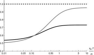
Figure 1: Left-hand side of Eq. (30) for hard spheres (black) and hard disks (gray). The horizontal dashed line, which is the upper bound of the inequality, is shown for reference. For $T\to 0$ one finds that this expression converges to $8/15=0.533\ldots$ for $d=3$ and to $21/22=0.9545\ldots$ for $d=2$, whereas for $T\to\infty$ it converges to $11/15=0.733\ldots$ for $d=3$ and to $1/2$ for $d=2$ (see App. A).

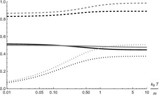
Figure 2: Characteristic speeds for hard spheres (black) and hard disks (gray). The solid, dashed and dotted lines refer to the speeds $\sqrt{\beta_{3}\eta}$, $\sqrt{\mu_{1}}$ and $\sqrt{\mu_{2}}$, respectively. The limits for $T\to 0$ and $T\to\infty$ can again be understood from the expressions provided in App. A.

V Stability and wave propagation

Next, we analyze the behavior of the solutions for wave lengths $\lambda$ satisfying $\ell_{mfp}\ll\lambda\ll\ell_{ms}$, with $\ell_{mfp}$ and $\ell_{ms}$ denoting the particles’ mean free path and the macroscopic scale, respectively. In this regime, it is possible to use the first-order theory and, at the same time, to freeze the coefficients as we have done in the previous section. It is illustrative to keep $\Gamma_{1}$ and $\Gamma_{2}$ arbitrary for the following analysis.

For transverse modes, one obtains from Eqs. (18) and (19) solutions of the form $U_{\perp}(t)=e^{st}U_{\perp}(0)$ with $s=s_{\pm}$ and

$$s_{\pm}=\frac{nh\beta_{3}}{2}\left[-1\pm\sqrt{1-\frac{4\eta k^{2}}{n^{2}h^{2}\beta_{3}}}\right].$$ (32)

Since $\eta/(nh),\,\kappa/(nh)\sim\ell_{mfp}$ one can expand the square root and obtain $s_{+}=-\frac{\eta k^{2}}{nh}+{\cal O}(\ell_{mfp}^{3}k^{4})$, whereas $s_{-}=-\frac{1}{\Gamma_{2}-1}\frac{nh}{\kappa}+{\cal O}(\ell_{mfp}k^{2})$. Provided $\Gamma_{2}>1$ (as required by hyperbolicity) the mode with $s_{-}$ is rapidly damped (on a time scale of $\ell_{mfp}$). The mode with $s_{+}$ has a slower damping time of the order of $1/(\ell_{mfp}k^{2})$ which is independent of $\Gamma_{1}$ and $\Gamma_{2}$ and corresponds to the shear channel [36, 37, 22]. Since $\mbox{Re}(s_{\pm})<0$ for all $k\neq 0$ the transverse system is stable.

Similarly, longitudinal modes are of the form $U_{\|}(t)=e^{st}U_{\|}(0)$ where $s$ is an eigenvalue of the $5\times 5$ matrix $P_{\|}:=ikM_{\|}+N_{\|}$. Explicitly, one finds

$$P_{\parallel}=\begin{pmatrix}0&0&0&-ik&0\\ 0&0&0&ik\alpha_{4}&ik\alpha_{5}\\ H_{0}\frac{k_{B}T\kappa}{h}&-H_{0}\frac{e\kappa}{h}&-H_{0}&2ik\eta\frac{d-1}{d}&-\frac{ik}{d}\\ ik\beta_{1}&ik\beta_{2}&ik\beta_{3}&0&0\\ 0&0&-ik&H_{1}\frac{\zeta}{\frac{k_{B}}{c_{v}}-\frac{1}{d}}&-H_{1}\end{pmatrix},$$ (33)

where we have abbreviated $H_{0}:=nh\beta_{3}$ and $H_{1}:=nTc_{v}\alpha_{5}$. After some calculations one finds that the characteristic polynomial of the matrix $P_{\|}$ has the following structure:

$$\begin{split}p(s)&:=\det\left(sI-P_{\|}\right)=s^{3}\left(s+H_{0}\right)\left(s+H_{1}\right)\\ &+k^{2}\left(c_{3}s^{3}+c_{2}s^{2}+c_{1}s\right)+k^{4}\left(d_{1}s+d_{0}\right),\end{split}$$ (34)

where the coefficients $c_{i}$ and $d_{i}$ are independent of $k$ and $s$ and can be found in App. B.

When $k=0$ one obtains the eigenvalues $0$ (three times degenerated) and $-H_{0}$ and $-H_{1}$. If $\Gamma_{1},\Gamma_{2}>1$, the last two yield modes that are rapidly damped, on time scales $\ell_{mfp}$. In order to investigate the behavior of the remaining modes for small values of $k$ we use perturbation theory (see App. B for details) and obtain eigenvalues of the form $s=-\frac{1}{\tau}\pm ivk+{\cal O}(\ell_{mfp}^{2}k^{3})$. There is a purely damped mode [37, 22], describing heat diffusion, for which

$$\frac{1}{\tau}=\frac{\kappa k^{2}}{nc_{p}T},\qquad v=0,$$ (35)

and two oscillating damped acoustic modes [36, 37, 22] for which

$$\frac{1}{\tau}=\frac{k^{2}}{2nh}\left[A+v^{2}\kappa\left(\frac{h}{c_{p}T}-1\right)^{2}\right],\quad v=\sqrt{\frac{k_{B}T}{h}\frac{c_{p}}{c_{v}}},$$ (36)

where $A:=2\left(1-\frac{1}{d}\right)\eta+\zeta$ is the Stokes attenuation coefficient and $c_{p}:=c_{v}+k_{B}$ the specific heat at constant pressure per particle. Therefore, the expected dynamics for low wave numbers is recovered.

Stability of the equilibrium configuration requires that $\mbox{Re}(s)<0$ for all $k\neq 0$. Based on the Routh-Hurwitz criterion [38, 39] one can prove that this is achieved, under the assumptions (i)-(iv) detailed in App. B, by setting

$$\Gamma_{1}=1+\frac{c_{v}}{k_{B}}\frac{e^{2}}{k_{B}Th}\left(\frac{k_{B}}{c_{v}}-\frac{1}{d}\right)^{2}\frac{\kappa}{\zeta}\Lambda_{0},$$ (37)

with large enough values of the constant $\Lambda_{0}$ and the choice (21) for $\Gamma_{2}$. In particular, the assumptions (i)-(iv) are satisfied for a simple gas of hard spheres or disks.

VI Final remarks and conclusions

In this work we proposed a new first-order theory of relativistic dissipative fluids based on the trace-fixed particle frame. We showed that this theory is hyperbolic and causal provided the single inequality (30) is satisfied. Moreover, we have specified sufficient conditions for global equilibria to be stable. Although similar in spirit to BDNK, our constitutive relations (4–6) are different from the ones in [23], as explained in the companion article [31]. In particular, the use of the trace-fixed particle frame, together with the freedom of choosing the temperature-dependent functions $\Gamma_{1}$ and $\Gamma_{2}$ according to Eqs. (21) and (37), naturally leads to a physically sound theory. The implications of the inequality (30) and the stability conditions need to be further explored. However, we have shown that there is at least one relevant case in which they are satisfied for all temperatures, namely for a simple gas consisting of hard disks or spheres. Furthermore, our theory reproduces correctly the known propagation of modes in the shear, acoustic and heat channels with low wave numbers. Finally, as shown in [31], our theory also implies positive entropy production within its limit of validity. Therefore, our system of equations should be well suited for a systematic study of transport phenomena in relativistic astrophysics, cosmology and high energy physics.

Appendix A Transport coefficients for hard disks and spheres

Here we summarize relevant formulas for a simple relativistic gas in $d=2,3$ space dimensions with a hard disk/sphere interaction model. For details and derivations see [34] for $d=3$ and [35] for $d=2$.

First, recall that the enthalpy per particle is given by [40]

$$h=m\mathcal{G}(z),\qquad\mathcal{G}(z):=\frac{K_{\frac{d+3}{2}}(z)}{K_{\frac{d+1}{2}}(z)},$$ (38)

where here and in the following, $m$ denotes the mass of the particles, $z:=m/(k_{B}T)$ and $K_{\nu}$ refer to the modified Bessel functions of the second type. Accordingly, the heat capacities at constant pressure and volume per particle are given by

$$c_{p}=-k_{B}z^{2}\mathcal{G}^{\prime}(z),\qquad c_{v}=c_{p}-k_{B},$$ (39)

where $\mathcal{G}^{\prime}$ denotes the derivative of $\mathcal{G}$. One can show that as the temperature $T$ increases from $0$ to $\infty$, $c_{v}$ increases monotonically from $d/2$ to $d$ and the quantity $\nu:=k_{B}T/e$ from $0$ to $1/d$.

From Eqs. (5.89-5.91) in [34] the transport coefficients for hard spheres in $d=3$ are, after translating to our notation,

$$\zeta =\frac{1}{64\pi}\frac{m}{z\sigma}\left[\frac{k_{B}}{c_{v}}\frac{d}{dz}\left(\frac{c_{v}}{k_{B}}\right)\right]^{2}\frac{z^{4}K_{2}(z)^{2}}{2K_{2}(2z)+zK_{3}(2z)},$$ (40)

$$\eta =\frac{15}{64\pi}\frac{m}{z\sigma}\frac{z^{4}K_{3}(z)^{2}}{(2+15z^{2})K_{2}(2z)+z(49+3z^{2})K_{3}(2z)},$$ (41)

$$\kappa =\frac{3}{64\pi}\frac{m}{z\sigma}\left(\frac{c_{p}}{k_{B}}\right)^{2}\frac{z^{2}K_{2}(z)^{2}}{(2+z^{2})K_{2}(2z)+5zK_{3}(2z)},$$ (42)

where $\sigma$ is the (constant) cross section. Consequently, the ratios

$$\frac{\zeta}{\kappa} =\frac{1}{3}\left[\frac{\frac{d}{dz}\left(z^{2}\mathcal{G}^{\prime}(z)\right)}{z\mathcal{G}^{\prime}(z)(1+z^{2}\mathcal{G}^{\prime}(z))}\right]^{2}\frac{2+z^{2}+5z\mathcal{G}(2z)}{2+z\mathcal{G}(2z)},$$ (43)

$$\frac{\eta}{\kappa} =5\left[\frac{\mathcal{G}(z)}{z\mathcal{G}^{\prime}(z)}\right]^{2}\frac{2+z^{2}+5z\mathcal{G}(2z)}{2+15z^{2}+z(49+3z^{2})\mathcal{G}(2z)},$$ (44)

are functions of the temperature only. In the non-relativistic limit $z\to\infty$ one finds $\mathcal{G}(z)=1+5/(2z)+\mathcal{O}(1/z^{2})$ and it follows that $\nu\eta/\kappa\to 4/15$ and $\nu\zeta/\kappa\to 0$, whereas in the ultrarelativistic limit, $\mathcal{G}(z)\sim 4/z$, which implies $\nu\eta/\kappa\to 1/5$ and $\nu\zeta/\kappa\to 0$. Using this information, one finds the following values for the characteristic speeds in the limit $T\to 0$:

$$\sqrt{\beta_{3}\eta} =\frac{2}{\sqrt{15}}\simeq 0.516,\quad\sqrt{\mu_{1}}=\sqrt{\frac{31}{45}}\simeq 0.830,$$

$$\sqrt{\mu_{2}} =0,$$ (45)

while for $T\to\infty$:

$$\sqrt{\beta_{3}\eta} =\frac{1}{\sqrt{5}}\simeq 0.447,\quad\sqrt{\mu_{1}}=\sqrt{\frac{7+2\sqrt{6}}{15}}\simeq 0.891,$$

$$\sqrt{\mu_{2}} =\sqrt{\frac{7-2\sqrt{6}}{15}}\simeq 0.374.$$ (46)

For $d=2$ one has $\mathcal{G}(z)=(z^{2}+3z+3)/(z(z+1))$ and for hard disks the transport coefficients are [35]

$$\zeta =\frac{15m}{R\mathcal{I}_{1}}\frac{1}{z^{2}\left(z^{2}+4z+2\right)^{2}},\quad\eta=\frac{30m}{R\mathcal{I}_{2}}\frac{\left(z^{2}+3z+3\right)^{2}}{z^{6}},$$

$$\kappa =\frac{15m}{R\mathcal{I}_{3}}\frac{(2z^{2}+6z+3)^{2}}{z^{6}\left(1+z\right)^{2}},$$ (47)

where $R$ is the radius of the disks and

$$\mathcal{I}_{1} =\int_{2z}^{\infty}\left(\frac{1}{x}+\frac{3}{x^{2}}+\frac{3}{x^{3}}\right)w(x,z)dx,$$ (48)

$$\mathcal{I}_{2} =\int_{2z}^{\infty}\left(x+2+\frac{3}{x}+\frac{3}{x^{2}}+\frac{3}{x^{3}}\right)w(x,z)dx,$$ (49)

$$\mathcal{I}_{3} =\int_{2z}^{\infty}\left(1+\frac{3}{x}+\frac{6}{x^{2}}+\frac{6}{x^{3}}\right)w(x,z)dx,$$ (50)

with $w(x,z):=\left(\frac{x^{2}}{z^{2}}-4\right)^{5/2}e^{-\left(x-2z\right)}$. Notice that, in order to obtain the thermal conductivity for the hard disks model, one needs to resort to the transformations established in Ref. [30] (see also Sec. IV in Ref. [41]). Indeed, since in Ref. [35] the heat flux is written as (translating to the notation and signature of the present work)

$$\mathcal{Q}^{\mu}=-\left(L_{T}\frac{D^{\mu}T}{T}+L_{n}\frac{D^{\mu}n}{n}\right),$$ (51)

one obtains $\kappa=\frac{h}{e}L_{T}$ which leads to the expression for $\kappa$ given by Eq. (A).

As in the three-dimensional case, the ratios $\zeta/\kappa$ and $\eta/\kappa$ are functions of the temperature only. For $z\to\infty$ one finds by means of the variable substitution $x=2z+\xi$ that

$$\mathcal{I}_{1}\sim\frac{30\sqrt{\pi}}{z^{7/2}},\qquad\mathcal{I}_{2}\sim\frac{120\sqrt{\pi}}{z^{3/2}},\qquad\mathcal{I}_{3}\sim\frac{60\sqrt{\pi}}{z^{5/2}},$$ (52)

which leads to $\nu\eta/\kappa\to 1/4$ and the following values for the characteristic speeds for $T\to 0$:

$$\sqrt{\beta_{3}\eta}=\frac{1}{2},\quad\sqrt{\mu_{1}}=\frac{\sqrt{3}}{2}\simeq 0.866,\quad\sqrt{\mu_{2}}=0.$$ (53)

For $z\to 0$ one finds

$$\mathcal{I}_{1}\sim\frac{48}{z^{5}},\qquad\mathcal{I}_{2}\sim\frac{1056}{z^{5}},\qquad\mathcal{I}_{3}\sim\frac{240}{z^{5}},$$ (54)

which yields $\nu\eta/\kappa\to 5/22$ and the following characteristic speeds for $T\to\infty$:

$$\sqrt{\beta_{3}\eta} =\sqrt{\frac{5}{22}}\simeq 0.477,\quad\sqrt{\mu_{1}}=\frac{1}{2}\sqrt{\frac{27+7\sqrt{5}}{11}}\simeq 0.985,$$

$$\sqrt{\mu_{2}} =\frac{1}{2}\sqrt{\frac{27-7\sqrt{5}}{11}}\simeq 0.508.$$ (55)

Appendix B Characteristic polynomial and stability

Here we provide details regarding the roots of the characteristic polynomial $p(s)$ defined in Eq. (33) of [42], which determines the complex frequencies of the longitudinal modes:

$$p(s) =s^{3}(s+H_{0})(s+H_{1})$$

$$+k^{2}\left(c_{3}s^{3}+c_{2}s^{2}+c_{1}s\right)+k^{4}\left(d_{1}s+d_{0}\right),$$ (56)

where $H_{0}=nh\beta_{3}$ and $H_{1}=nTc_{v}\alpha_{5}$. Explicitly, the coefficients $c_{i}$ and $d_{i}$ are given by

$$d_{0} = H_{0}H_{1}\frac{\kappa v_{s}^{2}}{nTc_{p}},$$ (57)

$$d_{1} = \frac{1}{d}\left[\kappa\beta_{3}-(1-\alpha_{4})\beta_{2}\right]+\alpha_{5}\beta_{2}A_{0},$$ (58)

$$c_{1} = H_{0}H_{1}v_{s}^{2},$$ (59)

$$c_{2} = \frac{H_{0}H_{1}}{nh}\left[A+\kappa\left(\frac{k_{B}T}{h}+\frac{e^{2}}{hTc_{v}}\right)\right]$$ (60)

$$+ (H_{0}+H_{1})v_{s}^{2},$$

$$c_{3} = \frac{1}{d}+\beta_{3}(\kappa+A_{0})-(1-\alpha_{4})\beta_{2},$$ (61)

where

$$v_{s}:=\sqrt{\frac{k_{B}T}{h}\frac{c_{p}}{c_{v}}},$$ (62)

is the speed of sound, $A_{0}:=2\left(1-\frac{1}{d}\right)\eta$, and $A:=A_{0}+\zeta$. Note that $d_{1}$ and $c_{3}$ are equal to the determinant $D$ and the trace $Tr$ of the matrix $RQ$, respectively. This can be understood by analyzing the behavior of the roots of $p(s)$ in the high-frequency limit. Indeed, considering $s=i\lambda k$ with $k\to\infty$, leads to

$$\lim\limits_{k\to\infty}\frac{p(s)}{k^{5}}=i\lambda(\lambda^{4}-c_{3}\lambda^{2}+d_{1}),$$ (63)

such that $\lambda^{2}$ are the eigenvalues of the matrix $RQ$. Before we proceed, we note that the coefficients $d_{0}$, $c_{1}$ and $c_{2}$ depend on the two paramters $\Gamma_{1}$ and $\Gamma_{2}$ of the theory only through the combinations $H_{0}H_{1}$ and $H_{0}+H_{1}$. This will play an important role in the following.

B.1 Behavior of the roots for small wave numbers

For small $|k|$ there are two roots of $p(s)$ which are of the form

$$s=-H_{0}+{\cal O}(\ell_{mfp}k^{2}),\quad s=-H_{1}+{\cal O}(\ell_{mdf}k^{2}),$$ (64)

and from now on we assume $\Gamma_{1},\Gamma_{2}>1$ such that $H_{0}$ and $H_{1}$ are positive which implies that these roots describe rapidly damped modes, as explained in the main text [42]. The other three roots are obtained from the ansatz $s=k^{r}y(k)$ with $y$ a smooth function of $k$ which converges to $y_{0}\neq 0$ as $k\to 0$. Substituting this ansatz into the characteristic polynomial gives

$$p(s) =k^{3r}y^{3}\left[H_{0}H_{1}+(H_{0}+H_{1})k^{r}y+k^{2r}y^{2}\right]$$

$$+k^{2+r}y\left(c_{1}+c_{2}k^{r}y+c_{3}k^{2r}y^{2}\right)+k^{4}\left(d_{0}+d_{1}k^{r}y\right).$$ (65)

We see from this that there are two possible values for $r$, namely $r=1$ and $r=2$. In the first case one obtains

$$0=\mathcal{F}(k,y) :=\frac{p(ky)}{k^{3}}=c_{1}y+H_{0}H_{1}y^{3}$$

$$+k\left[d_{0}+c_{2}y^{2}+(H_{0}+H_{1})y^{4}\right]+{\mathcal{O}}(k^{2}),$$ (66)

which in the limit $k\to 0$ yields

$$0=\mathcal{F}(0,y_{0})=y_{0}(c_{1}+H_{0}H_{1}y_{0}^{2}),$$ (67)

and, since $y_{0}\neq 0$ and $H_{0}H_{1}>0$, leads to

$$y_{0}=\pm i\sqrt{\frac{c_{1}}{H_{0}H_{1}}}=\pm iv_{s}.$$ (68)

Since

$$\frac{\partial\mathcal{F}}{\partial y}(0,y_{0})=c_{1}+3H_{0}H_{1}y_{0}^{2}=-2c_{1}<0,$$ (69)

the implicit function theorem guarantees, for small enough values of $|k|$, the existence of a smooth function $y(k)$ satisfying $\mathcal{F}(k,y(k))=0$ and $y(0)=y_{0}$. Differentiating both sides of Eq. (B.1) with respect to $k$ and evaluating at $k=0$ yields

$$y^{\prime}(0) =\frac{d_{0}+c_{2}y_{0}^{2}+(H_{0}+H_{1})y_{0}^{4}}{2c_{1}}$$

$$=-\frac{1}{2nh}\left[A+\kappa v_{s}^{2}\left(1-\frac{h}{Tc_{p}}\right)^{2}\right].$$ (70)

Hence, we obtain solutions for small $|k|$ of the form $s=\pm iv_{s}k+y^{\prime}(0)k^{2}+\mathcal{O}(k^{3})$ which lead to the damped acoustic modes described in Eq. (35) of the main text.

For $r=2$ one obtains from Eq. (B.1)

$$0=\mathcal{G}(k^{2},y) :=\frac{p(k^{2}y)}{k^{4}}=d_{0}+c_{1}y$$

$$+k^{2}\left[d_{1}y+c_{2}y^{2}+H_{0}H_{1}y^{3}\right]+{\mathcal{O}}(k^{4}).$$ (71)

For $k=0$ this yields $y_{0}=-\frac{d_{0}}{c_{1}}=-\frac{\kappa}{nc_{p}T}$, and since

$$\frac{\partial\mathcal{G}}{\partial y}(0,y_{0})=c_{1}>0,$$ (72)

the implicit function theorem guarantees again the existence of a smooth local solution $y(k^{2})$ of $\mathcal{G}(k^{2},y(k^{2}))=0$ such that $y(0)=y_{0}$. This gives rise to the damped heat diffusion modes described in Eq. (34) of the main text.

B.2 Mode stability for all wave numbers

To analyze the stability with respect to all wave numbers $k$, the Routh-Hurwitz criterion (see for instance [38, 39] for elementary proofs) is applied to the fifth-order polynomial Eq. (B) written as:

$$p(s)=s^{5}+a_{1}s^{4}+a_{2}s^{3}+a_{3}s^{2}+a_{4}s+a_{5},$$ (73)

with $a_{1}=H_{0}+H_{1}$, $a_{2}=H_{0}H_{1}+c_{3}k^{2}$, $a_{3}=c_{2}k^{2}$, $a_{4}=c_{1}k^{2}+d_{1}k^{4}$, $a_{5}=d_{0}k^{4}$. To ensure $\mbox{Re}(s)<0$ for all roots, it is essential that (i) $a_{i}>0$ for all $i=1,2,3,4,5$ and that (ii) the following inequalities are satisfied:

$$\det(H_{2}) :=a_{1}a_{2}-a_{3}>0,$$ (74)

$$\det(H_{3}) :=a_{3}\det(H_{2})-a_{1}(a_{1}a_{4}-a_{5})>0,$$ (75)

$$\det(H_{4}) :=a_{4}\text{det}(H_{3})-a_{5}(a_{1}a_{2}^{2}+a_{5}-a_{2}a_{3}-a_{1}a_{4})>0.$$ (76)

Explicitly, one finds

$$\det(H_{2}) =H_{0}H_{1}(H_{0}+H_{1})+B_{1}k^{2},$$ (77)

$$\det(H_{3}) =(H_{0}+H_{1})B_{2}k^{2}+\left[c_{2}B_{1}-(H_{0}+H_{1})B_{3}\right]k^{4},$$ (78)

$$\det(H_{4}) =(H_{0}+H_{1})\left[c_{1}B_{2}-d_{0}(H_{0}H_{1})^{2}\right]k^{4}$$

$$+\left[c_{1}c_{2}B_{1}-2c_{1}(H_{0}+H_{1})B_{3}+c_{2}H_{0}H_{1}B_{3}\right.$$

$$\left.-2d_{0}H_{0}H_{1}B_{1}\right]k^{6}+\left(c_{3}B_{1}B_{3}-B_{3}^{2}-d_{1}B_{1}^{2}\right)k^{8},$$ (79)

with

$$B_{1} =(H_{0}+H_{1})c_{3}-c_{2},\quad B_{2}=H_{0}H_{1}c_{2}-(H_{0}+H_{1})c_{1},$$

$$B_{3} =(H_{0}+H_{1})d_{1}-d_{0}.$$ (80)

In order to have $a_{i}>0$ and $\det(H_{i})>0$ for all $i=2,3,4$ and $k\neq 0$ (and keeping in mind that $H_{0}$ and $H_{1}$ are strictly positive) one is led to the following set of inequalities that must be fulfilled: $d_{0},d_{1},c_{1},c_{2},c_{3}>0$,

$$B_{1},B_{2}>0,$$ (81)

$$D_{1}:=c_{2}B_{1}-(H_{0}+H_{1})B_{3}>0,$$ (82)

$$D_{2}:=c_{1}B_{2}-d_{0}(H_{0}H_{1})^{2}>0,$$ (83)

$$D_{3}:=c_{3}B_{1}B_{3}-B_{3}^{2}-d_{1}B_{1}^{2}>0,$$ (84)

and

$$D_{4} :=(c_{1}c_{2}-2d_{0}H_{0}H_{1})B_{1}+\left[c_{2}H_{0}H_{1}\right.$$

$$\left.-2c_{1}(H_{0}+H_{1})\right]B_{3}>0.$$ (85)

(Alternatively, the last expression could be negative and suitably bounded from below to make sure that $\det(H_{4})>0$ for all $k\neq 0$; however we will not consider this option here.)

For the following, we analyze the validity of these conditions for the particular choice $\Gamma_{2}=h/(k_{B}T)$ which has $\beta_{1}=-\nu$, $\beta_{2}=0$ and $\beta_{3}=\nu/\kappa$, where we recall the definition $\nu:=\frac{k_{B}T}{e}$. In this case one finds $H_{0}=nh\nu/\kappa$ and

$$d_{0} =\nu\frac{H_{0}}{\Lambda}\frac{k_{B}}{c_{v}},\qquad d_{1}=\frac{\nu}{d},\qquad c_{1}=\frac{H_{0}^{2}}{\Lambda}v_{s}^{2},$$

$$c_{2} =H_{0}v_{s}^{2}+\frac{H_{0}}{\Lambda}\left(\nu+\nu\frac{A}{\kappa}+\frac{k_{B}}{c_{v}}\right),\quad c_{3}=\frac{1}{d}+\nu\left(1+\frac{A_{0}}{\kappa}\right),$$ (86)

where for simplicity we have set $\Lambda:=H_{0}/H_{1}$ which is positive. Explicitly, one finds

$$\Lambda=\frac{h}{e}\frac{k_{B}}{c_{v}}\left(\frac{k_{B}}{c_{v}}-\frac{1}{d}\right)^{-2}\frac{\zeta}{\kappa}(\Gamma_{1}-1),$$ (87)

such that choosing $\Gamma_{1}$ is equivalent to fixing $\Lambda$. In turn, the coefficients $B_{i}$ are given by

$$B_{1} =H_{0}\left[c_{3}-v_{s}^{2}-\frac{1}{\Lambda}\left(\frac{k_{B}}{c_{v}}-\frac{1}{d}+\nu\frac{\zeta}{\kappa}\right)\right],$$

$$B_{2} =\frac{H_{0}^{3}}{\Lambda^{2}}\left[\nu-v_{s}^{2}+\frac{k_{B}}{c_{v}}+\nu\frac{A}{\kappa}\right],$$

$$B_{3} =\nu H_{0}\left[\frac{1}{d}-\frac{1}{\Lambda}\left(\frac{k_{B}}{c_{v}}-\frac{1}{d}\right)\right].$$ (88)

For the following, we claim that when $\Lambda=\Lambda_{0}/\nu$ with a large enough constant $\Lambda_{0}$, the inequalities (81–85) are satisfied provided $e(T)$ and the the transport coefficients $\zeta$, $\eta$, and $\kappa$ satisfy the following conditions:

1. $e:(0,\infty)\to(m,\infty)$ is a smooth increasing function satisfying $e(T)\to m>0$ for $T\to 0$,

2. The heat capacity per particle $c_{v}=\frac{\partial e}{\partial T}$ is positive and converges to positive values for $T\to 0$ and $T\to\infty$,

3. The speed of sound satisfies the bounds $\nu\leq v_{s}^{2}\leq\frac{1}{d}$,

4. The quantities $\nu\frac{\eta}{\kappa}$ and $\nu\frac{\zeta}{\kappa}$ are bounded and $\nu\frac{\eta}{\kappa}$ converges to a positive value when $T\to\infty$.

These conditions are automatically fulfilled for a relativistic simple gas of hard spheres or disks (see the previous section). Recall also the condition $c_{v}<dk_{B}$ which, together with (i) and (ii), implies that

$$l_{0}:=\lim\limits_{T\to 0}\frac{v_{s}^{2}}{\nu}=\lim\limits_{T\to 0}\frac{e}{h}\frac{c_{p}}{c_{v}}=\lim\limits_{T\to 0}\frac{e}{h}\left(1+\frac{k_{B}}{c_{v}}\right)\geq 1+\frac{1}{d}>1.$$ (89)

In particular, it follows that $v_{s}\to 0$ for $T\to 0$ since $\nu\to 0$ in this limit. Furthermore, this and Eq. (89) show that condition (iii) is automatically satisfied for small temperatures. In the opposite limit, using L’Hôpital’s rule and condition (ii), one finds

$$l_{\infty}:=\lim\limits_{T\to\infty}\frac{v_{s}^{2}}{\nu}=\lim\limits_{T\to\infty}\frac{e}{h}\frac{c_{p}}{c_{v}}=\lim\limits_{T\to\infty}\frac{c_{v}}{c_{p}}\frac{c_{p}}{c_{v}}=1.$$ (90)

After these remarks we are ready to prove the claim. We first note that the coefficients $d_{i}$ and $c_{i}$ are positive. Next, using Eqs. (68,B.1) it is simple to verify that

$$0<-y^{\prime}(0)=\frac{D_{2}}{2c_{1}(H_{0}H_{1})^{2}},$$ (91)

such that the inequality (83) is automatically satisfied. Consequently, $B_{2}>0$, and hence it only remains to verify that $B_{1}$ and $B_{3}$ obey the inequalities $B_{1}>0$ and (82,84,85). In a next step, we introduce the quantities

$$g_{1}:=g_{3}+\nu\frac{\zeta}{\kappa},\qquad g_{3}:=\frac{k_{B}}{c_{v}}-\frac{1}{d},$$ (92)

which are bounded according to assumptions (ii) and (iv) and in terms of which

$$B_{1}=H_{0}\left(c_{3}-v_{s}^{2}-\frac{g_{1}}{\Lambda}\right),\qquad B_{3}=\nu H_{0}\left(\frac{1}{d}-\frac{g_{3}}{\Lambda}\right).$$ (93)

In particular, it follows that $B_{3}>0$ for large enough values of $\Lambda_{0}$. The positivity of $B_{1}$ is then a consequence of $D_{3}>0$. Using $c_{2}\geq H_{0}v_{s}^{2}$ one finds

$$D_{1} \geq H_{0}^{2}\left[P+\frac{1}{\Lambda}\left(\nu g_{3}-\frac{\nu}{d}-v_{s}^{2}g_{1}\right)+\frac{\nu g_{3}}{\Lambda^{2}}\right],$$ (94)

$$D_{3} = \frac{H_{0}^{2}\nu}{d}\left[P+\frac{(c_{3}-2v_{s}^{2})g_{1}+2\nu g_{3}-c_{3}(c_{3}-v_{s}^{2})g_{3}d}{\Lambda}+\frac{dg_{3}(c_{3}g_{1}-\nu g_{3})-g_{1}^{2}}{\Lambda^{2}}\right],$$ (95)

$$D_{4} \geq \frac{H_{0}^{4}}{\Lambda}\left[v_{s}^{2}P+\frac{\nu v_{s}^{2}\left(g_{3}-\frac{2}{d}\right)-2\nu\left(g_{3}+\frac{1}{d}\right)(c_{3}-v_{s}^{2})-v_{s}^{4}g_{1}}{\Lambda}+2\nu\frac{g_{1}\left(g_{3}+\frac{1}{d}\right)+v_{s}^{2}g_{3}}{\Lambda^{2}}\right],$$ (96)

where

$$P:=v_{s}^{2}(c_{3}-v_{s}^{2})-\frac{\nu}{d}=\left(\frac{1}{d}-v_{s}^{2}\right)(v_{s}^{2}-\nu)+2v_{s}^{2}\left(1-\frac{1}{d}\right)\nu\frac{\eta}{\kappa}.$$ (97)

According to the assumptions, $P>0$ for all $T>0$. Furthermore, using the limits (89,90) one finds

$$\lim\limits_{T\to 0}\frac{P}{\nu} \geq\frac{1}{d}(l_{0}-1)>0,$$

$$\lim\limits_{T\to\infty}\frac{P}{\nu} =2\left(1-\frac{1}{d}\right)\lim\limits_{T\to\infty}\nu\frac{\eta}{\kappa}>0.$$ (98)

Therefore, there exists a constant $\delta>0$ such that $P\geq\delta\nu$ for all $T>0$. Since the quantities $\nu$, $v_{s}^{2}$, $c_{3}$, $g_{1}$, $g_{3}$ and $\nu/v_{s}^{2}$ are bounded, there are constants $C_{ij}\geq 0$ such that

$$D_{i}\geq f_{i}\left[\delta-\frac{C_{i1}}{\Lambda_{0}}-\frac{C_{i2}}{\Lambda_{0}^{2}}\right],\qquad i=1,3,4,$$ (99)

with $f_{1}=H_{0}^{2}\nu$, $f_{3}=H_{0}^{2}\nu^{2}/d$ and $f_{4}=H_{0}^{4}v_{s}^{2}\nu/\Lambda$. Hence, by choosing $\Lambda_{0}$ sufficiently large one can guarantee that $D_{i}>0$ for all $i=1,3,4$ and the claim is proven.

Inverting the relation (87) and substituting $\Lambda=\Lambda_{0}/\nu$ leads to Eq. (36) in [42].