Density of states and differential entropy in the Dirac materials in crossed magnetic and in-plane electric fields

Abstract

The density of states and differential entropy per particle are analyzed for Dirac-like electrons in graphene subjected to a perpendicular magnetic field and an in-plane electric field. For comparison, the derived density of states is contrasted with the well-known case of nonrelativistic electrons in crossed magnetic and electric fields. The study considers ballistic electrons and also includes the effect of small impurity scattering. In the latter case, the limit of zero magnetic field and the so-called collapse of Landau levels in graphene are examined analytically. By comparing the results with numerical calculations on graphene ribbons, we demonstrate that the Landau state counting procedure must be modified for Dirac-like electrons, leading to a field-dependent Landau level degeneracy factor. Additionally, it is shown that peaks in the differential entropy arise from the dispersionless surface mode localized at the zigzag edges of the ribbon.

I Introduction

The entropy $S$ of many-body systems plays a fundamental role in characterizing their thermodynamic behavior, heat transfer, and thermoelectric properties. On the other hand, directly measuring entropy experimentally has always been challenging. Recently, however, it has been found that the differential entropy, $s\equiv\partial S/\partial n$, where $n$ is the electron density, can be investigated experimentally. Nevertheless, the experiment described in [1] is not an exception, as the quantity measured directly is actually the temperature derivative of the chemical potential, $\partial\mu/\partial T$. These derivatives are then equated using the Maxwell relation:

$$s=\left(\frac{\partial S}{\partial n}\right)_{T}=-\left(\frac{\partial\mu}{\partial T}\right)_{n}.$$ (1)

The differential entropy $s$ serves as an excellent thermodynamic tool, demonstrating high sensitivity in low charge density regimes, which allows for the study of two-dimensional electron gas (2DEG) in gated structures. In particular, in Ref. [1] the measurements of $s$ were performed in a quantizing perpendicular to 2DEG magnetic field $H$. The entropy showed a nonmonotonic dip-peak behavior as a function of $H$. As discussed in [2] (see also a recent review [3]) an intersection of the sequent Landau level and the chemical potential level can be viewed as an example of the Lifshitz electronic topological transition (ETT). Furthermore, measurements of differential entropy and integrated entropy change have revealed the isospin Pomeranchuk effect in magic-angle twisted bilayer graphene, as reported in Refs. [4, 5]. An important property of entropy per particle is its close relation to more complex transport properties, such as the Seebeck coefficient, making it a useful indicator for predicting the thermoelectric behavior of materials [6] (see also Refs. [7, 8, 9]).

Theoretical results for $s(\mu)$ indicate that it displays peak-dip structures associated with ETT in various 2D materials, such as gapped graphene monolayers [8], germanene [10], and semiconducting dichalcogenides [11] (see also the review [9]). It is shown in [12] that in the specific case of ETT occurring when the chemical potential crosses the saddle point in the dispersion, the differential entropy can be used to identify the type of associated van Hove singularity.

For an infinite system, the energies of the relativistic Landau levels in graphene subjected to a perpendicular magnetic field $H$ and an in-plane electric field $E$ are given by [13, 14]

$$\mathcal{E}_{n,k}=\mathcal{E}_{n}-\hbar k\frac{cE}{H},\quad\mathcal{E}_{n}=\pm(1-\beta^{2})^{3/4}\sqrt{2n}E_{M},$$ (2)

where $n=0,1,\ldots$, $k$ is the in-plane wave vector along the direction perpendicular to the electric field, $E_{M}=\hbar v_{F}/l$ is the magnetic energy scale with $l=\sqrt{\hbar c/(eH)}$ being the magnetic length, $\beta=v_{0}/v_{F}=cE/(v_{F}H)$, $v_{F}$ is the Fermi velocity and $v_{0}$ is the drift velocity. Here and in what follows we assume that $H>0$ and use CGS units.

As the dimensionless parameter $\beta$, which characterizes the strength of the electric field for a given magnetic field, approaches its critical value $|\beta_{c}|=1$, the Landau level staircase collapses into a single level [13, 14]. In an infinite system, this collapse can be interpreted as a transition from closed elliptic quasiparticle orbits when $|\beta|<1$ ($|v_{0}|<v_{F}$) to open hyperbolic orbits when $|\beta|>1$ ($|v_{0}|>v_{F}$) [15]. There is no Landau level collapse in ribbons because the orbit center cannot extend to infinity. Instead, the electron- and hole-like levels on opposite edges of the ribbon become denser, with the distance between them scaling as $O(l^{3}/W^{2})$, where $W$ is the ribbon width [16]. The presence of disorder inevitably causes the broadening of Landau levels, and as a result, these levels will merge due to their finite width.

It was shown in [17] that a delta-shaped transport distribution function maximizes the thermoelectric properties of a material. This result indicates a narrow distribution of the energy of the electrons participating in the transport. Consequently, it is reasonable to expect that the thermoelectric properties of Dirac materials will be enhanced as they approach the regime of Landau level collapse.

The aim of this study is to examine the behavior of entropy per particle $s$ in graphene subjected to crossed magnetic and in-plane electric fields, with a focus on how level convergence influences it. Since the calculation of $s$ relies on the density of states (DOS), the majority of this work is dedicated to the calculation and analysis of the DOS. The paper is organized as follows. In Sec. II, we overview the results for the density of states (DOS) in crossed fields for ballistic electrons in a nonrelativistic 2DEG [18, 19]. The notions of magnetic and electric regimes are introduced. A convenient for calculations analytical expression for the DOS that takes into account quasiparticle scattering is suggested. In Sec. III, the DOS for Dirac-like fermions is derived and analyzed using both analytical and numerical methods, with a discussion on the Landau level degeneracy factor. In Sec. IV we show how the entropy per particle dependence on the chemical potential is changing as the ratio of electric and magnetic fields changes both for analytical model which includes only the bulk Landau levels and numerical simulations on the ribbon which includes the dispersionless surface mode localized at the zigzag edges of the ribbon. Finally, the conclusions are given in Sec. V.

II DOS in the crossed fields: nonrelativistic case

II.1 Nonrelativisitic spectrum and general definition of the DOS

We begin by recapitulating the behavior of the DOS in crossed fields for ballistic electrons in a nonrelativistic 2DEG [18, 19]. The spectrum of nonrelativistic 2D electrons in a magnetic field $H$, perpendicular to the 2DEG plane, and an in-plane electric field $E$, directed along the $x$-axis, is given by [20]:

$$\begin{split}\mathcal{E}_{n,k_{y}}^{\mathrm{NR}}&=\mathcal{E}_{n}^{\mathrm{L}}-\frac{mc^{2}E^{2}}{2H^{2}}-\hbar k_{y}\frac{cE}{H},\\ \mathcal{E}_{n}^{\mathrm{L}}&=E_{M}^{\mathrm{NR}}\left(n+\frac{1}{2}\right),\end{split}$$ (3)

where as in Eq. (2) $n=0,1,\ldots$, $k_{y}$ is the in-plane wave vector along $y$ direction, $E_{M}^{\mathrm{NR}}=\hbar\omega_{c}$ is the nonrelativistic magnetic energy scale with $\omega_{c}=eH/(mc)$ being the cyclotron frequency and $m$ effective carrier mass, respectively. The spin splitting is omitted both in Eq. (3) and above in Eq. (2).

The full or integrated DOS per spin and unit area is defined as the sum over the complete set of the quantum numbers $\alpha=(n,k_{y})$ reads

$$D(\mathcal{E})=\frac{1}{\mathcal{A}}\sum_{\alpha}\delta(\mathcal{E}-\mathcal{E}_{\alpha})=\frac{L_{y}}{\mathcal{A}}\int\frac{dk_{y}}{2\pi}\sum_{n}\delta(\mathcal{E}-\mathcal{E}_{\alpha}).$$ (4)

We consider a system with dimensions $L_{x}$ and $L_{y}$, giving it an area of $\mathcal{A}=L_{x}L_{y}$.

In the absence of an electric field, $E=0$, the spectrum $\mathcal{E}_{n,k_{y}}^{\mathrm{NR}}$ simplifies to the standard Landau’s spectrum, $\mathcal{E}_{n}^{\mathrm{L}}$ given by the second line in Eq. (3). Exploiting the position-wave vector duality of Landau states, where the wave vector $k_{y}$ determines the center of the electron orbital along the $x$-axis, given by $x_{0}=-k_{y}l^{2}$, the DOS can be rewritten as follows:

$$D_{0}^{\mathrm{NR}}(\mathcal{E})=\frac{L_{y}}{\mathcal{A}}\int\frac{dx_{0}}{2\pi l^{2}}\sum_{n}\delta(\mathcal{E}-\mathcal{E}_{n}^{\mathrm{L}}).$$ (5)

Being independent of the quantum number $k_{y}$ the Landau levels are infinitely degenerate. As a consequence of this the DOS (5) is ill defined. The procedure for regularizing the number of states involves counting only the states within $-L_{x}/2\leq x_{0}\leq L_{x}/2$ and then taking the limit $L_{x}\to\infty$:

$$\lim_{L_{x}\to\infty}\frac{1}{L_{x}}\int dx_{0}\to\lim_{L_{x}\to\infty}\frac{1}{L_{x}}\int_{-L_{x}/2}^{L_{x}/2}dx_{0}=1.$$ (6)

This procedure is known as Landau state counting [21] (see also the textbook [22]) and yields the conventional expression for the DOS:

$$D_{0}^{\mathrm{NR}}(\mathcal{E})=\frac{1}{2\pi l^{2}}\sum_{n}\delta(\mathcal{E}-\mathcal{E}_{n}^{\mathrm{L}}).$$ (7)

Here

$$\mathfrak{g}_{L}=\frac{1}{2\pi l^{2}}=\frac{eH}{2\pi\hbar c}$$ (8)

is the usual degeneracy factor that corresponds to the number of states in the momentum space per one Landau level. Quasiclassically, it is defined as:

$$\mathfrak{g}=\frac{1}{(2\pi\hbar)^{2}}\int\int dp_{x}dp_{y}=\frac{S_{n+1}-S_{n}}{(2\pi\hbar)^{2}},$$ (9)

where the integration is done over neighboring classical trajectories and $S_{n}$ represents the orbit area in momentum space corresponding to the $n$-th Landau level. Evidently, the degeneracy (8) is recovered by taking $S_{n}=2\pi m\mathcal{E}_{n}^{\mathrm{L}}$.

Although the DOS (7) is derived by placing the electrons in a system of finite size, the Landau spectrum $\mathcal{E}_{n}^{\mathrm{L}}$ in Eq. (3) corresponds to an infinite system and does not take into account the surface electrons. Nevertheless, there is a consistency between the results obtained from Landau’s theory [21], essentially based on the DOS (7), and Teller’s approach [23], which accounts for the finite size of the system and the presence of the surface magnetization currents, as discussed in Ref. [24].

II.2 DOS in the crossed fields in the absence of scattering

In the presence of an electric field, the center of the electron orbit shifts as [20] $x_{0}=-k_{y}l^{2}-mc^{2}E/(eH^{2})$. Accordingly, the spectrum (3) in crossed fields can be expressed as follows:

$$\mathcal{E}_{n,x_{0}}^{\mathrm{NR}}=\mathcal{E}_{n}^{\mathrm{NR}}+eEx_{0},\quad\mathcal{E}_{n}^{\mathrm{NR}}=\mathcal{E}_{n}^{\mathrm{L}}+\Delta,\quad\Delta=\frac{mc^{2}E^{2}}{2H^{2}}\,.$$ (10)

Assuming that the orbit center falls within the range $-L_{x}/2\leq x_{0}\leq L_{x}/2$, we obtain the following DOS in crossed fields [18, 19]:

$$\begin{split}&D^{\mathrm{NR}}(\mathcal{E})=\frac{L_{y}}{\mathcal{A}}\int_{-L_{x}/2}^{L_{x}/2}dx_{0}D_{0}^{\mathrm{NR}}(\mathcal{E}-\Delta-eEx_{0})=\\ &\frac{\mathfrak{g}_{L}}{U}\sum_{n}\left[\theta(\mathcal{E}-\mathcal{E}_{n}^{\mathrm{NR}}+U/2)-\theta(\mathcal{E}-\mathcal{E}_{n}^{\mathrm{NR}}-U/2)\right].\end{split}$$ (11)

Here, the DOS defined by Eq. (7) is now written for the spectrum $\mathcal{E}_{n}^{\mathrm{NR}}$ given by Eq. (10) as taken into by the argument shift, $D_{0}(\mathcal{E}-\Delta)$, and $U=eEL_{x}$ is the potential difference between $x=-L_{x}/2$ and $x=L_{x}/2$. Here and in what follows, we assume for definiteness that $U>0$. Clearly, in the limit of a vanishing electric field, $U\to 0$, Eq. (11) reduces to its derivative with respect to $U$, returning to Eq.(7).

Note that in the presence of an electric field, the final result depends on the choice of integration limits for $x_{0}$, namely $-L_{x}/2\leq x_{0}\leq L_{x}/2$ or $0\leq x_{0}\leq L_{x}$, which leads to a shift in the levels due to the electric field [18, 19, 25]. For clarity in the presentation, we omit this shift and, from the outset, use symmetric integration limits for $x_{0}$.

II.3 Effect of elastic scattering

Elastic scattering of electrons by defects and impurities is inevitably present in real systems. A simple way to account for this smearing is by introducing a finite electron lifetime $\tau$. This broadens the Dirac delta function peaks associated with the Landau levels into Lorentzians with a constant, energy-independent width $\Gamma=\hbar/\tau$, as follows (see Ref. [26] for a detailed discussion):

$$\delta(\mathcal{E}-\mathcal{E}_{n})\to\frac{1}{\pi}\frac{\Gamma}{(\mathcal{E}-\mathcal{E}_{n})^{2}+\Gamma^{2}}.$$ (12)

Accordingly, for numerical computations based on Eq. (11), one can replace the Heaviside theta function $\theta(\mathcal{E}_{n})$ in the DOS (11) with

$$\tilde{\theta}(\mathcal{E})=\frac{1}{2}+\frac{1}{\pi}\arctan\frac{\mathcal{E}}{\Gamma}.$$ (13)

The Lorentzian approximation (12) allows us to derive a rather simple analytical expression from Eq. (7) for the DOS per spin and unit area in the absence of an electric field [27]

$$\begin{split}D_{0}^{\mathrm{NR}}(\mathcal{E})=-\frac{m}{2\pi^{2}\hbar}\mbox{Im}\psi\left(\frac{1}{2}-\frac{\mathcal{E}+i\Gamma}{E_{M}^{\mathrm{NR}}}\right)\\ =\frac{\mathfrak{g}_{L}}{\pi}\frac{d}{d\mathcal{E}}\mbox{Im}\ln\Gamma\left(\frac{1}{2}-\frac{\mathcal{E}+i\Gamma}{E_{M}^{\mathrm{NR}}}\right),\end{split}$$ (14)

where $\psi(z)$ and $\Gamma(z)$ are the digamma and gamma functions, respectively. It is clear that the peaks (oscillations) in the DOS are embedded in these functions when the real part of the argument becomes negative.

For a finite $\Gamma$ substituting Eq. (14) into the first line of Eq. (11), we obtain the DOS per unit area

$$\begin{split}D^{\mathrm{NR}}(\mathcal{E})=\frac{\mathfrak{g}_{L}}{\pi U}&\mbox{Im}\left[\ln\Gamma\left(\frac{1}{2}-\frac{\mathcal{E}-\Delta+U/2+i\Gamma}{E_{M}^{\mathrm{NR}}}\right)\right.\\ -&\left.\ln\Gamma\left(\frac{1}{2}-\frac{\mathcal{E}-\Delta-U/2+i\Gamma}{E_{M}^{\mathrm{NR}}}\right)\right].\end{split}$$ (15)

II.4 Illustrations of magnetic and electrical regimes

The characteristic cases of DOS (11) in crossed fields are presented in Figs. 1 and 2 for the scattering rate $\Gamma=0.001E_{M}^{\mathrm{NR}}$ and $\Gamma=0.05E_{M}^{\mathrm{NR}}$, respectively.

The linear in electric field shift of the levels is absent because of the choice of symmetric limits of integration in Eq. (11). The quadratic shift in the electric field by $\Delta$ present in $\epsilon_{n}$ [see Eq. (10)] is also omitted as in [19].

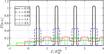
Figure 1: The DOS, $D^{\mathrm{NR}}(\mathcal{E})$, in crossed magnetic and electric fields versus energy $\mathcal{E}$ in units of $E_{M}^{\mathrm{NR}}=\hbar\omega_{c}$ for five values $\gamma=U/E_{M}^{\mathrm{NR}}$. The scattering rate $\Gamma=0.001E_{M}^{\mathrm{NR}}$.

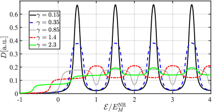
Figure 2: The DOS, $D^{\mathrm{NR}}(\mathcal{E})$, in crossed magnetic and electric fields versus energy $\mathcal{E}$ in units of $E_{M}^{\mathrm{NR}}$ for the same five values $\gamma=U/E_{M}^{\mathrm{NR}}$ as in Fig. 1. The scattering rate $\Gamma=0.05E_{M}^{\mathrm{NR}}$.

It can be seen that the presence of electric field destroys the sharp ($\delta$-like in the absence of scattering) peaks in the DOS. This occurs due to the $k_{y}$ dependence of the energies in Eq. (3). The parameter that controls the behavior of the DOS is the ratio of electric to magnetic energy, $\gamma=U/E_{M}^{\mathrm{NR}}=eEL_{x}/(\hbar\omega_{c})$. Accordingly, the regimes $\gamma<1$ and $\gamma>1$ are referred to as the magnetic and electric regimes, respectively [18, 19]. For $\gamma\ll 1$, the peaks in the DOS are well-defined, although their width is not related to the scattering rate $\Gamma$. For $\gamma\sim 1$, the peaks become lower and close to overlapping, and for $\gamma>1$, contributions from different subbands associated with the different Landau levels overlap significantly.

As was mentioned above, plotting Figs. 1 and 2 we omitted $\sim E^{2}/H^{2}$ shift of the energies. As follows from the energies $\mathcal{E}_{n}^{\mathrm{NR}}$ in Eq. (10) that the conduction subbands shift upwards as $E/H$ increases. On the other hand, using the equivalent form of the spectrum (3) which contains $-mc^{2}E^{2}/(2H^{2})-\hbar k_{y}cE/H$ and integrating over $k_{min}\leq k_{y}\leq k_{max}$ with $k_{min}=-k_{max}$, we obtain that the remaining conduction subband shifts downwards, when $E/H$ increases. Thus, depending on whether the $k_{y}$ dependence of the subbands is included in $x_{0}$ as in Eq. (10) or not, they shift upwards or downwards, at the rate $mc^{2}E^{2}/(2H^{2})$, respectively [18, 19]. As discussed in Refs. [18, 19], in the case of direct optical transitions, the value $k_{y}$ is conserved, that corresponds to the downward subband shift, which was observed experimentally. However, it is important to remember that in real samples, the broadening of DOS peaks due to the $k_{y}$ dependence of the energies is several orders of magnitude larger than the shift, allowing the latter to be neglected. As we will see later, the entire Landau state-counting procedure requires revision in the case of the collapsing Dirac spectrum (2). This issue will be revisited in the next section.

II.5 DOS in the limit of vanishing magnetic field

An advantage of the analytic representations (14) (15) is that it allows to access the limit of vanishing magnetic field, $H\to 0$. Using the asymptotic expansions

$$\psi(z)=\ln z-\frac{1}{2z}-\frac{1}{12z^{2}}+O\left(\frac{1}{z}\right)^{4},\qquad z\to\infty,$$ (16)

and

$$\begin{split}\ln\Gamma(z)=&\left(z-\frac{1}{2}\right)\ln z-z+\frac{1}{2}\ln(2\pi)\\ &+\frac{1}{12z}-\frac{1}{360z^{3}}+O\left(\frac{1}{z}\right)^{4},\qquad z\to\infty,\end{split}$$ (17)

and also taking $\Gamma\to 0$ limit, one obtains, respectively, the DOS

$$D_{0}^{\mathrm{NR}}(\mathcal{E})=\begin{cases}0,&\mathcal{E}<0,\\ \frac{m}{2\pi\hbar^{2}},&\mathcal{E}>0,\end{cases}$$ (18)

and

$$D^{\mathrm{NR}}(\mathcal{E})=\begin{cases}0,&\mathcal{E}\leq-U/2,\\ \frac{m}{2\pi\hbar^{2}}\frac{U+2\mathcal{E}}{2U},&-U/2\leq\epsilon\leq U/2,\\ \frac{m}{2\pi\hbar^{2}},&\mathcal{E}\leq U/2.\end{cases}$$ (19)

Eq. (18) is nothing but the free electron DOS per spin in 2D that confirms consistency of Landau state counting. The result (19) is also consistent with the corresponding expressions from Refs. [18, 19], where it was derived for the case of zero magnetic field and a finite electric field.

III DOS in the crossed fields: case of graphene

III.1 DOS in the crossed fields in the absence of scattering

The key difference between the spectrum (2) and the 2DEG spectrum (3) is that the Dirac Landau levels are not equidistant. Consequently, as we will see below, the parameter $\gamma=eEL_{x}/E_{M}$, with

$$E_{M}=\hbar v_{F}/l\equiv\sqrt{\hbar v_{F}^{2}eH/c},$$ (20)

which characterizes the ratio of electric to magnetic energies, cannot globally distinguish between the magnetic and electric regimes across all energy levels.

Using Eq. (9) with $S_{n}=\pi\mathcal{E}_{n}^{2}/v_{F}^{2}$, we find that this factor becomes dependent on $\beta$ and is expressed as:

$$\mathfrak{g}(\beta)=\mathfrak{g}_{L}(1-\beta^{2})^{3/2}.$$ (21)

This dependence was not accounted for in previous work [25, 28]. As we will demonstrate, using the Landau degeneracy factor $\mathfrak{g}_{L}$ instead of $\mathfrak{g}(\beta)$ leads to unphysical behavior in the DOS. In what follows we will show that our choice of $\mathfrak{g}(\beta)$ is consistent both with numerical calculations performed on ribbons and with the zero field DOS.

Thus by substituting the Dirac spectrum (2) into the definition (4), integrating over the wave number $-L_{x}/(2l^{2})\leq k_{y}\leq L_{x}/(2l^{2})$, and taking into account the proposed degeneracy factor (21), we obtain the DOS for both valleys per spin:

$$\begin{split}D(\mathcal{E})=\frac{2\mathfrak{g}(\beta)}{U}\sum_{n}&\left[\theta(\mathcal{E}-\mathcal{E}_{n}+U/2)\right.\\ &-\left.\theta(\mathcal{E}-\mathcal{E}_{n}-U/2)\right],\end{split}$$ (22)

where as above $U=eEL_{x}$. Note that the method of integrating over wave numbers $k_{y}$ used here corresponds to the procedure described at the end of Sec. II.4. An alternative approach could involve integrating over the orbit center position $x_{0}$, which, in the case of Landau level collapse in an infinite system, is given by [13, 16]:

$$x_{0}=-k_{y}l^{2}-\frac{\beta l\,\text{sgn}(\mathcal{E}_{n})\sqrt{2n}}{(1-\beta^{2})^{1/4}}.$$ (23)

The different choices of integration limits reflect the difficulties with the Landau state counting procedure, especially in the presence of electric field. In such cases, the geometric parameter $L_{x}$ enters the final result through the electric potential difference $U$. As mentioned above, the procedure adopted here ensures agreement with numerical results obtained for sufficiently wide ribbons, where the portion of the spectrum within the ribbon aligns with the spectrum (2) for an infinite system.

It is helpful to rewrite the DOS (22) in terms of the dimensionless parameter $\gamma$ as follows:

$$\begin{split}D(\epsilon)=\frac{2\mathfrak{g}(\beta)}{E_{M}\gamma}\sum_{n}&\left[\theta(\epsilon-\epsilon_{n}(\beta)+\gamma/2)\right.\\ &-\left.\theta(\epsilon-\epsilon_{n}(\beta)-\gamma/2)\right],\end{split}$$ (24)

where the energy is measured in the units of $E_{M}$

$$\epsilon_{n}(\beta)\equiv\mathcal{E}_{n}/E_{M}=\pm(1-\beta^{2})^{3/4}\sqrt{2n},\quad n=0,1,\ldots$$ (25)

By expressing the electric energy as $U=\beta\hbar v_{F}/l^{2}L_{x}$, we see that the parameters $\gamma$ and $\beta$ are related by

$$\gamma=\beta L_{x}/l.$$ (26)

Thus, varying $\beta$ leads to changes in $\gamma$. It is more convenient to consider both parameters as independent variables. This can be achieved by assuming that, for fixed values of $\beta$, variations in $\gamma$ are obtained by adjusting the width $L_{x}$. Similarly, one can assume that $L_{x}$ is adjusted to keep $\gamma$ constant as $\beta$ changes.

III.2 Peculiarities of magnetic and electric regimes in the Dirac Landau level case

To illustrate the role of $\gamma$ in the Dirac Landau level case, it is convenient to start by setting $\beta=0$ in Eq. (25) and examining how the DOS behaves as the value of $\gamma$ varies in Eq. (24). Recall that level broadening can be incorporated by replacing $\theta(\epsilon)$ with $\tilde{\theta}(\epsilon)$, as defined by Eq. (13).

In Fig. 3, we present the DOS (24) for $-1\leq\epsilon\leq 4$.

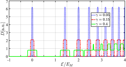
Figure 3: The DOS, $D(\mathcal{E})$, in crossed magnetic and electric fields versus energy $\mathcal{E}$ in units of $E_{M}$ for three values $\gamma=U/E_{M}$. The scattering rate $\Gamma=0.001E_{M}$.

Note that with symmetric integration limits, the DOS remains an even function of $\epsilon$, as in the zero electric field case. Thus, here and in what follows, we plot the DOS over a representative energy range. The curves for smaller values, $\gamma=0.05$ and $\gamma=0.15$, within the shown energy range, correspond to the magnetic regime. The peaks’ centers align with the positions of the Landau levels, given by $\epsilon(\beta=0)=\pm\sqrt{2n}$. The widening of the levels is due to the $k_{y}$ dependence of the level energies, rather than the Landau level width $\Gamma=0.001E_{M}$, which is chosen to be rather small. For the larger value of $\gamma=0.4$, levels with $n>2$ begin to overlap, indicating that the system has entered the electric regime.

In general, the condition for the overlap of levels $\mathcal{E}_{n+1}$ and $\mathcal{E}_{n}$ is given by:

$$\mathcal{E}_{n+1}-\mathcal{E}_{n}=U.$$ (27)

This leads to the condition

$$\sqrt{n+1}+\sqrt{n}=\frac{\sqrt{2}(1-\beta^{2})^{3/4}}{\gamma}$$ (28)

which, for $n\gg 1$, simplifies to

$$n\simeq\frac{(1-\beta^{2})^{3/2}}{2\gamma^{2}}.$$ (29)

For $\gamma=0.4$, the last equation yields $n\simeq 3.1$, which we observe despite this being a relatively low value for the level index $n$.

In Fig. 4 we show the DOS (24) for the same two values of $\gamma=0.15$ and $\gamma=0.4$ as above in Fig. 3, but for a wider range of energies $0\leq\epsilon\leq 10$. One can see that while in Fig. 3 the red corresponding to $\gamma=0.15$ remained in the magnetic regime, in Fig. 4 the same curve now enters electric regime for $n\gtrsim 22$ in agreement with Eq. (29). Furthermore, the curve for $\gamma=0.4$, which enters the electric regime even at low energies $\epsilon\gtrsim 2.5$, exhibits an interesting pattern as the energy increases. We observe a step-like increase in the DOS, with each step containing oscillations of the same amplitude. As we will discuss in relation to Fig. 6, this behavior is associated with the overlap of three or more Landau levels.

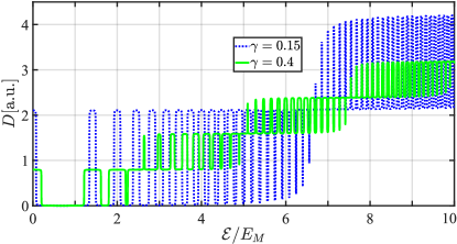
Figure 4: The DOS, $D(\mathcal{E})$, in crossed magnetic and electric fields versus energy $\mathcal{E}$ in units of $E_{M}$ for two values $\gamma=U/E_{M}$. The scattering rate $\Gamma=0.001E_{M}$.

Fig. 5 is calculated for the same values of $\gamma$ and the same range of energies as Fig. 4, but with a Landau level width $\Gamma$ that is 50 times larger. This results in the smearing of the DOS for larger values of $\epsilon$ and as we will see below its behavior resembles the DOS in the absence of the magnetic field.

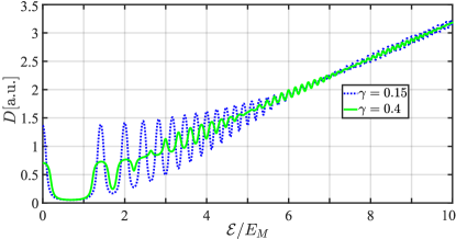
Figure 5: The DOS, $D(\mathcal{E})$, in crossed magnetic and electric fields versus energy $\mathcal{E}$ in units of $E_{M}$ for the same two values of $\gamma=U/E_{M}$ as in 4. The scattering rate $\Gamma=0.05E_{M}$.

We now return to the DOS envelope steps observed in Fig. 4. In Fig. 6 we again plot the DOS for $\gamma=0.4$, but with additional vertical lines to clarify the observed behavior. The solid (magenta) lines correspond to the positions of the unperturbed by electric field Landau levels given by Eq. (25) for $\beta=0$. We recall that Figs. 3 – 6 are plotted for $\beta=0$. The dashed (green) lines demarcate the boundaries of the regions with the different number of overlapping Landau levels: the region with $N=1$ corresponds to a single contributing level, for $N=2$ two overlapping levels contribute to the DOS.

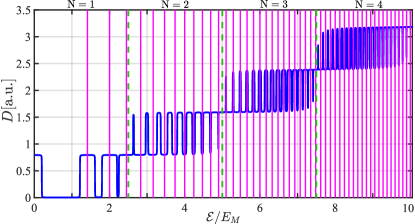
Figure 6: The DOS, $D(\mathcal{E})$, in crossed magnetic and electric fields versus energy $\mathcal{E}$ in units of $E_{M}$ for $\gamma=U/E_{M}=0.4$. The scattering rate $\Gamma=0.001E_{M}$. The solid (magenta) vertical lines show the positions of the Landau levels $\epsilon_{n}(\beta=0)$ given by Eq. (25). The dashed (green) vertical lines demarcate the boundaries of the regions with the different number of overlapping Landau levels.

III.3 Analytic representations of the DOS

It is useful to obtain the analytic representation of the DOS in terms of the $\ln\Gamma(z)$ function in the crossed fields for the Dirac Landau level case, because it allows for the study of the DOS in the Landau level collapse regime. Assuming, as in Eq. (14), that all Landau levels have the same width $\Gamma$ as described by Eq. (12) and the spectrum, $\mathcal{E}_{n}(\beta=0)$ is given by Eq. (2), the following representation for the DOS per spin in the absence of an electric field was derived in [26]

$$\begin{split}&D_{0}(\mathcal{E},E_{M})=\frac{1}{\pi^{2}\hbar^{2}v_{F}^{2}}\left\{\Gamma\ln\frac{\Lambda^{2}}{2E_{M}^{2}}-\right.\\ &\left.\mbox{Im}\left[(\mathcal{E}+i\Gamma)\left(\psi\left(\frac{-(\mathcal{E}+i\Gamma)^{2}}{2E_{M}^{2}}\right)-\frac{E_{M}^{2}}{(\mathcal{E}+i\Gamma)^{2}}\right)\right]\right\}\\ &=\frac{1}{\pi^{2}\hbar^{2}v_{F}^{2}}\left[\Gamma\ln\frac{\Lambda^{2}}{2E_{M}^{2}}+E_{M}^{2}\frac{d}{d\mathcal{E}}\right.\\ &\left.{\rm Im}\left[\ln\Gamma\left(\frac{-(\mathcal{E}+i\Gamma)^{2}}{2E_{M}^{2}}\right)+\frac{1}{2}\ln\left(\frac{-(\mathcal{E}+i\Gamma)^{2}}{2E_{M}^{2}}\right)\right]\right..\end{split}$$ (30)

Here, $\Lambda$ represents the energy cutoff, which is required due to the use of the Dirac approximation for the dispersion. The zero magnetic field, $E_{M}\to 0$, limit of Eq. (30) reproduces the known expressions for the DOS. In particular, using the asymptotic (16) we obtain [26] in the clean limit ($\Gamma\to 0$):

$$D_{0}(\mathcal{E})=\frac{|\mathcal{E}|}{\pi\hbar^{2}v_{F}^{2}},$$ (31)

while in the presence of impurities we reproduce the expression from [29]

$$D_{0}(0)=\frac{2\Gamma}{\pi^{2}\hbar^{2}v_{F}^{2}}\ln\frac{\Lambda}{\Gamma}.$$ (32)

It is easy to see that for the collapsing spectrum $\mathcal{E}_{n}(\beta)$ and the degeneracy factor $\mathfrak{g}(\beta)$, the result can be obtained simply by replacing $E_{M}\to E_{M}(1-\beta^{2})^{3/4}$. Similarly to the nonrelativistic DOS (15), the DOS (per unit area) in crossed fields can be expressed in terms of the DOS (30) for a magnetic field only, where the representation involving the derivative with respect to the energy $\mathcal{E}$ is particularly useful for integration

$$D(\mathcal{E})=\frac{1}{L_{x}}\int_{-L_{x}/2}^{L_{x}}dx_{0}D_{0}(\mathcal{E}+eEx_{0},E_{M}(1-\beta^{2})^{3/4}),$$ (33)

where we used $x_{0}=-k_{y}l^{2}$. Then we obtain the following expression for the DOS

$$\begin{split}D(\mathcal{E})=&\frac{1}{\pi^{2}\hbar^{2}v_{F}^{2}}\Gamma\ln\frac{\Lambda^{2}}{2E_{M}^{2}(1-\beta^{2})^{3/2}}\\ &+\frac{2\mathfrak{g}(\beta)}{\pi U}[d(\mathcal{E}+U/2)-d(\mathcal{E}-U/2)],\end{split}$$ (34)

where the function

$$\begin{split}d(\mathcal{E})=&{\rm Im}\left[\ln\Gamma\left(\frac{-(\mathcal{E}+i\Gamma)^{2}}{2E_{M}^{2}(1-\beta^{2})^{3/2}}\right)\right.\\ &+\left.\frac{1}{2}\ln\left(\frac{-(\mathcal{E}+i\Gamma)^{2}}{2E_{M}^{2}(1-\beta^{2})^{3/2}}\right)\right]\end{split}$$ (35)

Analogously to the nonrelativistic case, the representation in (34) allows for an analytical investigation when the argument $z$ of the $\Gamma(z)$ function approaches infinity, using the asymptotic expansion (17). While in the nonrelativistic case this regime corresponds to the $H\to 0$ limit, for graphene, it can be reached by either taking $E_{M}\to 0$ or $|\beta|\to 1$. For the case of Landau level collapse, let us focus on the second limit. Assuming further that the width $\Gamma\to 0$, we obtain the following result

$$D(\mathcal{E})=\frac{1}{\pi\hbar^{2}v_{F}^{2}}\begin{cases}|\mathcal{E}|,&|\mathcal{E}|>U/2,\\ \frac{\mathcal{E}^{2}+U^{2}/4}{U},&|\mathcal{E}|\leq U/2.\end{cases}$$ (36)

It can be observed that for $|\mathcal{E}|>U/2$, the DOS matches the free ($H=E=0$) DOS of graphene, as given by Eq. (31). This occurs because the corrected degeneracy factor $\mathfrak{g}(\beta)$ eliminates the $(1-\beta^{2})^{-3/2}$ divergence in the DOS that would otherwise arise [25, 28].

For $|\mathcal{E}|\leq U/2$, the merging of Landau levels alters the linear energy dependence of $D(\mathcal{E})$ to a parabolic one. Additionally, the zero-energy DOS becomes finite and depends on the applied electric field, given by $D(0)=U/(4\pi\hbar^{2}v_{F}^{2})$. Note that when a finite value of $\Gamma$ is considered, the DOS given by Eq. (32) must be added to Eq. (36), showing that the product $E_{M}^{2}(1-\beta^{2})^{3/2}$ in the denominator of the first term of Eq. (34) is properly canceled out in this limit. This indicates that the electric field plays a similar role to $\Gamma$, making the zero energy DOS nonzero

The equation (36) can also be rewritten for $\epsilon=\mathcal{E}/E_{M}$, so that

$$D(\epsilon)=\frac{E_{M}}{\pi\hbar^{2}v_{F}^{2}}\begin{cases}|\epsilon|,&|\epsilon|>\gamma/2,\\ \frac{\epsilon^{2}+\gamma^{2}/4}{\gamma},&|\epsilon|\leq\gamma/2.\\ \end{cases}$$ (37)

To conclude the discussion of Eqs. (36) and (37), it should be noted that although these equations were derived under the conditions $|\beta|\to 1$ or $E_{M}\to 0$, they are also applicable in cases where the ratio of electric to magnetic energy, $\gamma$ is large and $|\mathcal{E}|\ll U$. This is because, in such case, the argument of $\Gamma(z)$ in Eqs. (34) and (35) also becomes significantly large.

III.4 Numerical simulations of the DOS

The spectrum was computed using the software “Kwant” [30]. The system is modeled as a graphene honeycomb lattice, configured as an infinite nanoribbon with zigzag edges. The ribbon has a defined width along the $x$-direction and extends infinitely along the $y$-direction. To explore the electronic properties, we applied an electric field along the ribbon’s width, perpendicular to its length characterized by the potential $V(\mathbf{r})=eEx$. In this case, it is convenient to consider the magnetic field in the following Landau gauge $(A_{x},A_{y})=(0,Hx)$, where $H$ is the magnitude of a constant magnetic field orthogonal to the ribbon’s plane. Therefore, the wave functions are plane waves in the $y$ direction $\sim\exp(ik_{y}y)$, where as before $k_{y}$ is a continuous quantum number, which is numerically discretized for computational purposes. By introducing the boundary conditions at the zigzag edges, we compute the energy spectrum $\mathcal{E}_{n,k_{y}}$. Unlike the spectrum in Eq. (2), this spectrum has a finite number of Landau levels characterized by the discrete Landau level index $n$, owing to the finite number of atoms along the $x$-direction.

Overall, the entire described procedure numerically implements Teller’s approach [23] for describing electrons in a magnetic field within a finite geometry. This approach avoids the issues inherent in Landau’s method [21], which uses eigenfunctions and eigenenergies derived from an infinite system to analyze the free energy in a finite geometry [24]. Accordingly, the DOS per unit area and spin is defined as:

$$D(\mathcal{E})=\frac{1}{L_{x}}\sum_{n}\int_{BZ}\frac{dk_{y}}{2\pi}\delta\left(\mathcal{E}-\mathcal{E}_{n,k_{y}}\right),$$ (38)

where the eigenenergies $\mathcal{E}_{n,k_{y}}$ are determined numerically, the integration is performed over the first Brillouin zone in the corresponding direction, and the summation accounts for the Landau level index $n$. This approach avoids the issues associated with Landau state counting, as discussed below Eq. (5). For the numerical calculation, the $\delta$-functions in the DOS, Eq. (38) were regularized by introducing finite energy level width in the form of Lorentzian shape given by Eq. (12). The width $\Gamma$ is taken to be much smaller than the characteristic energy scale, defined by the hopping parameter $t$, and smaller than temperature $T$, to keep important features from being hidden.

An example of such a spectrum, along with the corresponding DOS, is presented in Fig. 7.

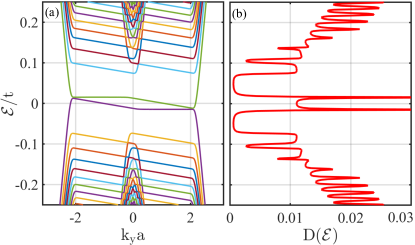
Figure 7: (a) Energy spectrum $\mathcal{E}_{n,k_{y}}$ computed for the tight binding model for a hexagonal lattice subjected to a magnetic field $H=$54.5\text{\,}\mathrm{T}$$ (or $l=14.1a$ where a is the triangular lattice spacing) for a system size of width $L_{x}=500a$. The plot shows $\mathcal{E}_{n,k_{y}}$ in the units of the hopping parameter $t$ as function of $k_{y}a$, where $k_{y}$ is the wave vector in the $y$ direction. An external electric field $E$ applied along $x$ axis, given by the parameter $\beta=cE/(v_{F}H)=-0.014$. (b) The DOS, $D(\mathcal{E})$, is calculated based on the depicted spectrum. The energy $\mathcal{E}$ in the units of $t$.

Overall, the presented spectrum is consistent with existing lattice computations, such as those in Ref. [13] (see also Ref. [31] for a review). Since the ribbon is sufficiently wide ($L\approx 35l$), the spectrum corresponds to the bulk Landau levels described by Eq. (2). The electric field induces a linear $k_{y}$ dependence in the bulk Landau levels and causes a constant shift in the edge states. Additionally, dispersionless states, which are surface states localized at the zigzag boundaries, are also present. It was shown in Ref. [32] by analytic methods that these states remain unaffected by the presence of an electric field. The energy distance between the dispersionless levels is $U$ and they show up in the DOS [Fig. 7 (b)] as the peaks at $\mathcal{E}=\pm U/2$. The wider peaks associated with the broadening by electric field and starting to overlap higher Landau levels are also seen in Fig. 7 (b).

To look closer at these features in Fig. 8 (a) and (b) we plot against each other the results of the calculations based on Eq. (24) and numerical simulations, respectively, for three different values of electric field (or $\beta$) and the same ribbon’s width $L_{x}=500a\approx 35l$.

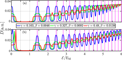
Figure 8: The DOS, $D(\mathcal{E})$, in crossed magnetic and electric fields versus energy $\mathcal{E}$ in units of $E_{M}$ for $\beta=0.0046$, $\gamma=0.163$ blue curve; $\beta=0.0046$, $\gamma=0.163$ blue curve $\beta=0.0092$, $\gamma=0.327$ green curve; and $\beta=0.0139$, $\gamma=0.49$. The magnetic field $H=$54.5\text{\,}\mathrm{T}$$, and ribbon width equals $L_{x}=500a=35.4l$ for all curves. The scattering rate $\Gamma=0.01t=0.0163E_{M}$. The solid (magenta) vertical lines show the positions of the bulk Landau levels $\epsilon_{n}(\beta=0)$ given by Eq. (25). (a) Calculated based on Eq. (24). (b) Numerical simulations on the lattice.

Recall that for a fixed $L_{x}$, an increase in $\beta$ leads to an increase in $\gamma$, as shown in Eq. (26). The peaks in the blue curve, calculated for the smallest electric field, align with the positions of the bulk Landau levels in the Dirac approximation, Eq. (25), indicated by the solid (magenta) vertical lines. However, even for the $n=3$ Landau level, the peak positions in Fig.8 (b), obtained from lattice calculations, are slightly shifted from the values predicted by Eq.(25). This is expected, as the large magnetic field ($H=$54.5\text{\,}\mathrm{T}$$) results in the energy of the $n=5$ level, $\sqrt{5}E_{M}\approx 0.3t$, deviating from the Dirac approximation. Nevertheless, for the first two levels even for the largest value of $\beta$ shown in the red curve, the agreement between the Dirac approximation and lattice simulations remains qualitative.

Now using the simulations we test the introduced in Eq. (21) the dependent on $\beta$ the Landau level degeneracy factor $\mathfrak{g}(\beta)$. In Fig. 9 (a) and (b) we plot against each other the results of the calculations based on Eq. (24) and numerical simulations, respectively, for three different values of $\gamma$ and the fixed $\beta$. In accordance to Eq. (26) the variation of $\gamma$ is reached by changing the ribbon’s width $L_{x}$.

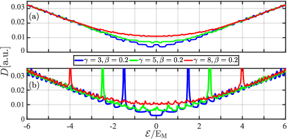
Figure 9: The DOS, $D(\mathcal{E})$, in crossed magnetic and electric fields versus energy $\mathcal{E}$ in units of $E_{M}$ for $\beta=0.2$ and three different values of $\gamma$: $\gamma=3$ blue curve; $\gamma=5$ green curve; and $\gamma=8$ red curve. The magnetic field value is $H=$54.5\text{\,}\mathrm{T}$$ and the scattering rate $\Gamma=0.01t=0.0163E_{M}$. (a) Calculated based on Eq. (24). (b) Numerical simulations on the lattice.

The peaks associated with the dispersionless levels are at $\pm\gamma/2$ are seen in Fig. 9 (b), but absent in Fig. 9 (a) which is computed by taking into account only the bulk Landau levels. However, except for these peaks, there is a good agreement between the results obtained from Eq. (24) and numerical simulations. The DOS between the peaks is parabolic and described by Eq. (37).

To see this Fig. 10 we plot together the DOS given by Eq. (37) (black curve) and numerical simulations, respectively, for three different values of $\beta$ and the fixed $\gamma$.

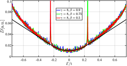
Figure 10: The DOS, $D(\mathcal{E})$, in crossed magnetic and electric fields versus energy $\mathcal{E}$ in units of the hopping parameter $t$ by numerical simulations for $\gamma=8$ and three different values of $\beta$ : $\beta=0.5$ blue curve; $\beta=0.75$ green curve; and $\beta=0.75$ The magnetic field value is $H=$54.5\text{\,}\mathrm{T}$$ and the scattering rate $\Gamma=0.001t=0.0163E_{M}$. The black curve is the DOS given by Eq. (37).

In accordance with Eq. (26) the variation of $\beta$ is reached by changing the ribbon’s width $L_{x}$. We observe that the simulation results for different values of $\beta$ are nearly identical and align well with Eq. (37). It is important to emphasize that the DOS described by Eq. (37) is independent of $\beta$. However, if the factor $(1-\beta^{2})^{3/2}$ were not included in the degeneracy factor given by Eq. (21), the three theoretical curves corresponding to different values of $\beta$ would deviate significantly. Such discrepancies would contradict the numerical simulations.

For $|\epsilon|\geq\gamma/2$ the parabolic behavior observed in the numerical simulations transforms to a linear one, in agreement with Eq. (37). However, as $|\epsilon|$ continues to increase, the linear behavior in the numerical curves becomes nonlinear once again. This occurs for $|\epsilon|\gtrsim 0.3t$, where the Dirac approximation is no longer applicable.

IV Differential entropy

As mentioned in the Introduction, the differential entropy $s$, also known as entropy per particle, is directly related to the temperature derivative of the chemical potential at a fixed electron density $n(\mu,T)$ (see Eq. (1)). The latter can be obtained using the thermodynamic identity

$$\left(\frac{\partial\mu}{\partial T}\right)_{n}=-\left(\frac{\partial n}{\partial T}\right)_{\mu}\left(\frac{\partial n}{\partial\mu}\right)_{T}^{-1}.$$ (39)

At thermal equilibrium, the total density of electrons is

$$n(T,\mu)=\int_{-\infty}^{\infty}d\epsilon D(\epsilon)f_{\rm{FD}}\left(\frac{\epsilon-\mu}{T}\right),$$ (40)

where $f_{\rm{FD}}(x)=1/[\exp(x)+1]$ is the Fermi-Dirac distribution function and we set the Boltzmann constant to $k_{B}=1$ and measure the temperature in energy units. Note that, in the presence of electron-hole symmetry, it is convenient to work with the difference between electron and hole densities rather than the total electron density, as is commonly done for graphene [8].

Differentiating Eq. (40) with respect to $T$ and $\mu$ respectively, results in the well-known expression for the differential entropy [7, 8, 9]

$$s(\mu,T)=\frac{1}{T}\frac{\int_{-\infty}^{\infty}d\varepsilon\,D(\varepsilon)(\varepsilon-\mu)\cosh^{-2}\left(\frac{\varepsilon-\mu}{2T}\right)}{\int_{-\infty}^{\infty}d\varepsilon D(\varepsilon)\,\cosh^{-2}\left(\frac{\varepsilon-\mu}{2T}\right)}.$$ (41)

Using Eq. (41), it is clear that the extrema in the dependence of $D(\mu)$ corresponds to the zeros of $s(\mu)$. Since van Hove singularities produce sharp peaks in the DOS, they appear as characteristic features in the dependence of $s(\mu)$ discussed in [12], followed by pronounced peak and dip structures [7, 8, 9].

There is a similarity between Eq. (41) and the corresponding expression for the Seebeck coefficient $\mathcal{S}$, such that, for an energy-independent relaxation time, they are identical. The relationship between $\mathcal{S}$ and $s$ in zigzag graphene ribbons without external fields was analyzed in detail in [6], where it was shown that within the gap, $\mathcal{S}\simeq s/e$, with $e$ as the electron charge and the Boltzmann constant restored in $s$.

In Fig. 11 we plot differential entropy as a function of chemical potential $\mu$ for the bulk states only.

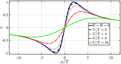
Figure 11: The differential entropy $s$ versus the chemical potential $\mu$ in the units of $T$. The solid (black) curve is for the free $H=E=0$ case; the dashed (blue), $U=2T$; the dotted (grey), $U=4T$; the dash-dotted (red), $U=8T$; thick solid (green), $U=16T$.

The reference case $H=E=0$, where the free DOS given by Eq. (31), is shown by the solid (black) curve and analytically is described by the following expression [8]

$$\begin{split}s&=\frac{1}{\ln\left(2\cosh\frac{\mu}{2T}\right)}\left[\mbox{Li}_{2}\left(-e^{-\frac{\mu}{T}}\right)-\mbox{Li}_{2}\left(-e^{\frac{\mu}{T}}\right)\right]-\frac{\mu}{T}.\end{split}$$ (42)

Here Li is the polylogarithm function. One can also extract the asymptotics of Eq. (42) both for $|\mu|\ll T$ and $|\mu|\gg T$ [8]. In particular, the latter limit if multiplied by the factor $k_{B}/e$ agrees with the Seebeck coefficient for a free electron gas. It should also be noted that the differential entropy is independent of whether the DOS is calculated using the degeneracy factor $\mathfrak{g}(\beta)$ or $\mathfrak{g}_{L}$. The other curves in Fig. 11 were computed using the DOS (36) in the collapse limit and for large $\gamma$. As the value of $U$ given in the units of the temperature $T$ increases, these curves become less steep, reflecting a more smooth behaviour of the DOS.

Next, we analyze the behavior of $s(\mu)$ for small values of $\gamma$, where the lowest Landau levels remain distinct and do not overlap. In Fig. 12 we plot the DOS and the corresponding differential entropy $s$ as a function of chemical potential at two values of the temperature $T=0.08E_{M}$ and $T=0.2E_{M}$ in four cases: $\gamma=0$ ($E=0$), $\gamma=0.5$, $\gamma=1$ and $\gamma=2$.

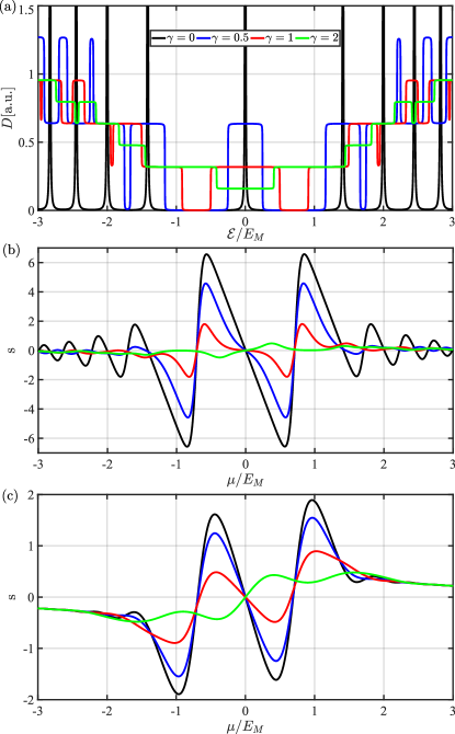
Figure 12: The DOS, $D(\mathcal{)}$, and differential entropy $s(\mu)$ for four values of $\gamma$: $\gamma=0$ black curve; $\gamma=0.5$ blue curve; $\gamma=1$ red curve; and $\gamma=2$ green curve. (a) The DOS, $D(\mathcal{E})$ versus energy $\mathcal{E}$ in units of $E_{M}$. (b) The differential entropy $s$ versus the chemical potential $\mu$ in the units of $E_{M}$, for $T=0.08E_{M}$ (c) The same as (b), but for for $T=0.2E_{M}$.

The DOS, $D(\mathcal{E})$ in Fig. 12 (a) is computed using Eq. (22) [see also Eq. (24)]. As in Sec. 22 for convenience of comparison, we set $\beta=0$. The case marked as $\gamma=0$ corresponds to the $\gamma\to 0$ limit when the results in the in graphene under a magnetic field alone are recovered. The value $\Gamma=0.001E_{m}$ is taken. The dependence $s(\mu)$ exhibits oscillations and features a sharp peak when the chemical potential is near the Dirac point, $|\mu|\sim T$, within the temperature range. The amplitude of the oscillations is higher for the lower value of $T=0.08E_{M}$. We observe that as the value of $\gamma$ increases, these features become less pronounced. Note that for $\gamma=2$, when the $n=0$ and $n=1$ levels begin to overlap, the corresponding green curve crosses the $\mu=0$ point from negative to positive values of $s$. In contrast, curves with smaller values of $\gamma$ cross this point from positive to negative values of $s$.

Finally, in Fig. 13 we show the dependence $s(\mu)$ computed for the DOS presented in Fig. 7 (b).

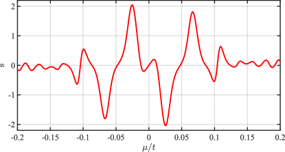
Figure 13: The differential entropy $s$ versus the chemical potential $\mu$ in the units of $t$, for $T=0.003t=0.049E_{M}$ and $U=0.03t$, with scattering rate $\Gamma=0.001t=0.0163E_{M}$, calculated by numerical simulations on the lattice.

Overall the behavior of $s(\mu)$ is similar to the results presented in Fig. 12, with one significant exception. The DOS peaks at $\mathcal{E}=\pm U/2\approx\pm 0.015t$, associated with the dispersionless surface states, introduce an additional dip-peak structure near $\mu=0$.

V Conclusion

One can estimate that for a magnetic field of $H=$1\text{\,}\mathrm{T}$$ and the Fermi velocity $v_{F}=$1\text{\times}{10}^{6}\text{\,}\mathrm{m}\mathrm{/}\mathrm{s}$$, the critical electric field is $E_{c}=$1\text{\times}{10}^{4}\text{\,}\mathrm{V}\mathrm{/}\mathrm{c}\mathrm{m}$$, which is achievable experimentally. For example, with $H=$0.1\text{\,}\mathrm{T}$$, the magnetic length is approximately $l\approx$82\text{\,}\mathrm{nm}$$. For a ribbon of width $L_{x}=20l\approx$1.6\text{\,}\mathrm{\SIUnitSymbolMicro m}$$, this corresponds to a critical voltage between the ribbon edges of $U=$0.16\text{\,}\mathrm{V}$$. Indeed, experimental studies have reported the realization of Landau level collapse [33, 34]. Another potential approach to achieve Landau level collapse is by generating strain-induced pseudomagnetic or electric fields, as proposed in Refs. [35, 36]. This demonstrates that the results for the DOS and differential entropy presented in this work are accessible for experimental investigation.

It would be particularly interesting to explore how the behavior of the DOS can be adjusted by applying an in-plane electric field, given its relevance from both research and practical perspectives. From a research point, it is crucial to confirm that the Landau degeneracy factor $\mathfrak{g}_{L}$ [see Eq. (8)] for graphene in the crossed fields must be replaced with the electric field-dependent factor $\mathfrak{g}(\beta)$, as defined in Eq. (21). It would also be useful to study the degeneracy factor in other similar situations. From a practical perspective, enhancing the DOS by tuning the in-plane electric field could be valuable for achieving greater control over the transport properties of graphene.

Using the results for the DOS, we analyzed the behavior of the differential entropy. Since the energy dependence of the DOS, for bulk states, becomes smoother, the differential entropy exhibits a less steep variation compared to the $H=E=0$ case. When the lowest Landau levels do not overlap, the dependence $s(\mu)$ exhibits oscillations and features a sharp peak when the chemical potential is near the Dirac point. Further investigation is warranted to understand how the dip-peak structure observed in $s(\mu)$ near $\mu=0$, associated with the dispersionless surface states, manifests in the Seebeck coefficient.