Non-BCS behavior of the pairing susceptibility near the onset of superconductivity in a quantum-critical metal

Abstract

We analyze the dynamical pairing susceptibility $\chi_{pp}(\omega_{m})$ at $T=0$ in a quantum-critical metal, where superconductivity emerges out of a non-Fermi liquid ground state once the pairing interaction exceeds a certain threshold. We obtain $\chi_{pp}(\omega_{m})$ as the ratio of the fully dressed dynamical pairing vertex $\Phi(\omega_{m})$ and the bare $\Phi_{0}(\omega_{m})$ (both infinitesimally small). For superconductivity out of a Fermi liquid, the pairing susceptibility is positive above $T_{c}$, diverges at $T_{c}$, and becomes negative below it. For superconductivity out of a non-Fermi liquid, the behavior of $\chi_{pp}(\omega_{m})$ is different in two aspects: (i) it diverges at the onset of pairing at $T=0$ only for a certain subclass of bare $\Phi_{0}(\omega_{m})$ and remains non-singular for other $\Phi_{0}(\omega_{m})$, and (ii) below the instability, it becomes a non-unique function of a continuous parameter $\phi$ for an arbitrary $\Phi_{0}(\omega_{m})$. The susceptibility is negative in some range of $\phi$ and diverges at the boundary of this range. We argue that this behavior of the susceptibility reflects a multi-critical nature of a superconducting transition in a quantum-critical metal when immediately below the instability an infinite number of superconducting states emerges simultaneously with different amplitudes of the order parameter down to an infinitesimally small one.

I Introduction

Pairing of incoherent fermions out of a non-Fermi liquid ground state is a fascinating subject that attracted significant attention over the last three decades. Examples of such pairing include fermions at half-filled Landau levels [1, *Monien1993, *Nayak1994, *Altshuler1994, *Kim_1994, 6], quantum-critical metals at the onset of various spin and charge orders [7, 8, 9, 10, 11, *acs2, *finger_2001, *acn, 15, *Subir2, *Sachdev2019, 18, *Sachdev_22, 20, 21, *efetov2, *efetov3, *benlagra2011luttinger, 25, *metlitski2010quantum2, *max_2, *max_last, 29, *sslee_2018, 31, 32, *ital2, *ital3, 20, *wang23, 36, *wang_22, 38, *berg_2, *berg_3, *Hu2017, *berg_4, *meng, 44, *peter, 46, *tsvelik, *tsvelik_1, *tsvelik_2, *tsvelik_3, 51, *DellAnna2006, 53, *metzner_1, *metzner_2, 56, 57, *Yang2011, 59, 60, 61, 62, *Wu_19, 64, *avi1, *avi2, *avi_5, 68, 69, *foster], electron-phonon systems at small Debye frequency [71, *scal, 73, *ad, *combescot, 76, *boyack, 78, *Chubukov_2020b, 80, 81, 82, *emil1, *emil2, *emil3, *emil4, 87, *math_3, 89, *berg_a], SYK-type systems [91, 92, 93, 94, 95, 96], e.g., quantum dots, and systems near a van Hove singularity, particularly a higher-order one [97, *Chamon, *Risto]. Rich physics here comes from the fact that non-Fermi liquid and superconductivity are competing phenomena. Namely, a fermionic incoherence in a non-Fermi liquid weakens the system’s ability to create fermionic pairs and develop a coherent supercurrent. At the same time, if superconductivity develops, the associated gap opening reduces the scattering at low energies and renders fermionic coherence. The outcome of the competition depends on the interplay between the interaction in the particle-hole and particle-particle channels as the first gives rise for a non-Fermi liquid while the second gives rise to pairing. In most cases, the two interactions originate from the same effective 4-fermion interaction between low-energy fermions and are comparable in strength. In this situation, non-Fermi liquid and superconductivity compete on equal footing. In the quantum-critical models studied so far [100, *raghu2, *raghu3, *Fitzpatrick_15, 104, *Subir2, 105, 106, *paper_2, *paper_3, *paper_4, *paper_5, *paper_6, *odd, *jetp, 114] superconductivity wins, but by purely numerical reasons.

In this communication we consider a more generic case, when the interactions in the particle-hole and particle-particle channel have the same functional form, but differ by some factor. Such a situation emerges [100] upon extension of the original $SU(2)$ model to matrix $SU(N)$ with $N\gg 1$: the interaction in the particle-particle channel becomes smaller by the factor of $N$. A similar situation holds in Yukawa-SYK models with the only difference that the relative smallness of the particle-particle interaction is controlled by a continuous parameter – the strength of time-reversal symmetry breaking disorder [92, 93, 94, 96]. In our study we follow these earlier works. We label the ratio of the two interactions by $1/N$, in analogy with the $SU(N)$ case, but treat $N$ as a continuous parameter, like in Yukawa-SYK models.

To simplify the presentation, we focus on superconductivity in a metal near a quantum-critical point. Earlier studies[100, *raghu2, *raghu3, *Fitzpatrick_15, 115, 105, 106, *paper_2, *paper_3, *paper_4, *paper_5, *paper_6, *odd, *jetp, 116, 117, *Wang_H_18, 114] of quantum-critical metals have found that to a good accuracy (analytical in some cases, numerical in others) the competition between non-Fermi liquid and superconductivity in a spatial channel with the highest attraction can be can described by an effective Eliashberg-type theory with local dynamical interaction $V(\Omega_{m})$, local self-energy $\Sigma(\omega_{m})$ and local pairing vertex $\Phi(\omega_{m})$ (all three are real functions of frequency on the Matsubara axis). A more familiar superconducting gap function $\Delta(\omega_{m})$ is related to $\Phi(\omega_{m})$ as $\Delta(\omega_{m})=\Phi(\omega_{m})/(1+\Sigma(\omega_{m})/\omega_{m})$. These earlier studies have shown that at $T=0$ there exists a critical $N_{cr}$ separating regions of a non-Fermi liquid ground state at $N>N_{cr}$ and a superconducting state at $N<N_{cr}$ (see Fig. 1). A conventional wisdom would then tell that the dynamical pairing vertex $\Phi(\omega_{m})$ is zero at $N>N_{cr}$, is infinitesimally small at at $N=N_{cr}-0$, and is finite at $N<N_{cr}$ with magnitude increasing with deviation from $N_{cr}$. The actual situation is, however, more complex as it turns out that $N=N_{cr}$ is a multi-critical point, below which an infinite number of topologically distinct solutions $\Phi_{n}(\omega)$ appears simultaneously with $n=0,1,2...$ (Refs. [106, 119, *son_2, *son_3, 96] The function $\Phi_{n}(\omega_{m})$ has $n$ zeros along the Matsubara axis in the upper half-plane of frequency. The magnitude of $\Phi_{n}(\omega_{m})$ decreases with $n$ and becomes infinitesimally small at $n\to\infty$ for any $N<N_{cr}$. This implies that the linearized equation for $\Phi(\omega_{m})$ has a solution not only at $N=N_{cr}-0$ but also for arbitrary $N<N_{cr}$, along with an infinite set of solutions of the non-linear gap equation.

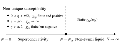
Figure 1: A schematic zero-temperature phase diagram of the $\gamma$-model, extended to $N>1$. A non-Fermi liquid phase with a positive and non-singular pairing susceptibility holds for $N>N_{\text{cr}}$, and a superconducting phase holds for $N<N_{\text{cr}}$. In the latter, the pairing susceptibility is non-unique. The critical value $N_{\text{cr}}$ varies with $\gamma$ between $N_{cr}=\infty$ at $\gamma=0$ and $N_{cr}=1$ for $\gamma=1$.

This highly unconventional behavior calls for the analysis of the pairing susceptibility, $\chi_{pp}(\omega_{m})$. We define $\chi_{pp}$ as the system reaction to an infinitesimally small input $\Phi_{0}(\omega_{m})$, i.e., as $\chi_{pp}(\omega_{m})=\Phi(\omega_{m})/\Phi_{0}(\omega_{m})$, where $\Phi(\omega_{m})$ is the fully dressed response function – the solution of the gap equation induced by $\Phi_{0}(\omega_{m})$. In a BCS superconductor, $\chi_{pp}(\omega_{m})=\chi_{pp}$ is frequency independent. It is positive in the normal state, diverges at the critical point, and becomes negative below the critical point, indicating that the normal state is unstable towards pairing. In the quantum-critical case, the susceptibility has to reflect the fact that at $\Phi_{0}=0$ and $N<N_{cr}$, there exist a set of solutions with a finite $\Phi_{n}(\omega_{m})$, for which one could expect a negative but finite pairing susceptibility, and the solution with infinitesimally small $\Phi_{\infty}(\omega_{m})$, for which one would expect the susceptibility to diverge. The goal of our work is to reconcile these two seemingly different forms of the susceptibility.

We will also explain another unconventional feature of the pairing susceptibility, detected in earlier studies by comparing the quantum-critical pairing with the BCS case [10, 106, 113]. Namely, in BCS theory, the pairing susceptibility is obtained by summing up ladder series of Cooper logarithms at a finite temperature $T$. The series are geometrical and sum up into $\chi_{pp}\propto 1/\log{T/T_{c}}$ implying that it diverges at $T=T_{c}$. For the quantum-critical case, the ladder series for $\chi_{pp}$ at $T=0$ are also logarithmic and contain powers of $\log{|\omega_{m}|}$ due to a combination of singular interaction and singular self-energy (we will present explicit expressions below). However, the ladder series are not geometrical and sum up into a power-law form $\chi_{pp}(\omega_{m})\propto\left(\frac{1}{|\omega_{m}|}\right)^{\frac{1-\gamma}{N}}$. There is no indication in this formula that a superconducting instability develops at $N=N_{cr}$. We argue that an instability can be detected, but one has to analyze the validity of perturbation theory.

In this work, we first consider the case when the bare $\Phi_{0}(\omega_{m})=\Phi_{0}$ is independent on frequency. We show that the behavior of the pairing susceptibility is highly unconventional: it does not diverge as $N$ approaches $N_{cr}$ from above and remains finite and positive at $N=N_{cr}$. However, once $N$ gets smaller than $N_{cr}$ the perturbative expansion in $\log{|\omega_{m}|}$ breaks down. To see this, we will go beyond the leading logarithms and collect non-logarithmic corrections in powers of $1/N$ for each term in the logarithmic series. We show that at $N>N_{cr}$, the pairing susceptibility becomes the function not only of frequency but also of a running parameter $\eta$. For a particular value of $\eta=\pi/2$, $\chi_{pp}(\omega_{m},\pi/2)$ diverges for all $\omega_{m}$, consistent with the existence of an infinitesimally small $\Phi_{\infty}(\omega_{m})$. For the range of $\eta$ near $\pi/2$, the pairing susceptibility is finite, but negative, consistent with the existence of the set of finite $\Phi_{n}(\omega_{m})$.

We next analyze in detail a generic case when the input infinitesimal $\Phi_{0}$ is a function of frequency, $\Phi_{0}(\omega_{m})$. We show that the behavior is generally the same as for a constant $\Phi_{0}$, i.e., there is an abrupt change of $\chi_{pp}$ at $N=N_{cr}$ from a regular function of frequency to a function of two variables - frequency and a running parameter. However for a set of $\Phi_{0}(\omega_{m})$, $\chi_{pp}$ diverges as $N$ approaches $N_{cr}$ from above, and at $N<N_{cr}$ again becomes a function of a running parameter.

The outline of the paper is the following. In the next section we present the model and the set of coupled equations for the pairing vertex and the self-energy. We briefly describe the results obtained by solving these equations without the source term and then present the equation for the pairing susceptibility. In Sec. III we analyze the pairing susceptibility for the case when the source term $\Phi(\omega_{m})=\Phi_{0}$ in independent on frequency. We show that the pairing susceptibility remains finite for $N\geq N_{cr}$, and becomes a multi-valued function at $N<N_{cr}$. In Sec. IV we extend the analysis to frequency dependent $\Phi_{0}(\omega_{m})$. We show that for a generic $\Phi_{0}(\omega_{m})$ the behavior of the susceptibility is similar to the case of a constant $\Phi_{0}$, but for a special $\Phi_{0}(\omega_{m})$, the pairing susceptibility diverges at $N\to N_{cr}$ from above, and again becomes a multi-valued function at $N<N_{cr}$. In Sec. V we present the explanation of the behavior of the pairing susceptibility at $N\geq N_{cr}$ by invoking the criterium of normalizability of $\Phi(\omega_{m})$ and show that in physical terms it implies that the condensation energy must remain finite. We present our conclusions in Sec. VI.

II Model and gap equation

In a quantum critical metal the dynamical interaction between fermions $V(\Omega_{m})=(g/|\Omega_{m}|)^{\gamma}$ is mediated by massless fluctuations of a collective bosonic degree of freedom in either spin or charge channel (the $\gamma-$model, named by he exponent). As we said, we assume that the interactions in particle-hole and particle-particle channels have the same functional form, but the latter an extra factor $1/N$.

Taken alone, the interaction in the particle-particle channel gives rise to a superconducting ground state with a non-zero $\Phi(\omega_{m})$, whose spatial symmetry is specified by the underlying microscopic model (e.g., $d-$wave for the quantum-critical metal at the onset of an antiferromagnetic order). In turn, the interaction in the particle-hole channel, taken alone, gives rise to a non-Fermi liquid ground state with the self-energy

$$\Sigma(\omega_{m}) = \text{sign}(\omega_{m})\Sigma^{*}(\omega_{m}),$$

$$\Sigma^{*}(\omega_{m}) = \int_{0}^{|\omega_{m}|}V(\Omega_{m})d\Omega_{m}=|\omega_{m}|^{1-\gamma}\omega^{\gamma}_{0}$$ (1)

where $\omega_{0}=g/(1-\gamma)^{1/\gamma}$. Below we will measure the self-energy, the pairing vertex, and frequency in units of $\omega_{0}$, i.e., redefine $\Sigma(\omega_{m})\to\omega_{0}\Sigma(\omega_{m})$, $\Phi(\omega_{m})\to\omega_{0}\Phi(\omega_{m})$, and $\omega_{m}\to\omega_{m}/\omega_{0}$.

The ground state of the $\gamma$ model in the presence of both interactions has been analyzed before. To address the interplay between superconductivity and non-Fermi liquid, one has to solve the set of two coupled non-linear equations for the pairing vertex and the self-energy:

$$\Phi(\omega_{m})=\frac{1-\gamma}{2N}\int\frac{d\omega^{{}^{\prime}}_{m}\Phi(\omega^{{}^{\prime}}_{m})}{\sqrt{\left(\omega^{{}^{\prime}}_{m}+\Sigma(\omega^{{}^{\prime}}_{m})\right)^{2}+\Phi^{2}(\omega^{{}^{\prime}}_{m})}}\frac{1}{|\omega_{m}-\omega^{{}^{\prime}}_{m}|^{\gamma}}$$

$$\Sigma(\omega_{m})=\frac{1-\gamma}{2}\int\frac{d\omega^{{}^{\prime}}_{m}\Sigma(\omega^{{}^{\prime}}_{m})}{\sqrt{\left(\omega^{{}^{\prime}}_{m}+\Sigma(\omega^{{}^{\prime}}_{m})\right)^{2}+\Phi^{2}(\omega^{{}^{\prime}}_{m})}}\frac{1}{|\omega_{m}-\omega^{{}^{\prime}}_{m}|^{\gamma}}$$

(2)

Similar, though not identical equations have been obtained for the Yukawa SYK model of dispersion-less fermions, interacting with Einstein phonons, in the limit when the number of fermionic and bosonic flavors tend to infinity, but their ratio is finite.

Eqs. (2) have been analyzed before[106], both analytically and numerically. We do not discuss the details and just list the results, which will serve as an input for the analysis of the susceptibility. These results are different for $0<\gamma<1$ and $\gamma>1$ (Ref. [109] For definiteness, we focus on $0<\gamma<1$.

• At large $N>N_{cr}$, the ground state remains a non-Fermi liquid, i.e., $\Phi(\omega_{m})=0$, and the self-energy is given by (1).

• At $N<N_{cr}$, the ground state is a superconductor with $\Phi(\omega_{m})\neq 0$. The feedback from superconductivity renders the Fermi liquid form of the self-energy.

• The value of $N_{cr}$ depends on the exponents $\gamma$ as

  $$N_{cr}=\left(\frac{1-\gamma}{2}\right)\frac{\Gamma^{2}\left(\frac{\gamma}{2}\right)}{\Gamma\left(\gamma\right)}\left(1+\frac{1}{\cos{\left(\frac{\pi\gamma}{2}\right)}}\right)$$ (3)

  At small $\gamma$, $N_{cr}\approx 4(1-\gamma)/\gamma$; at $\gamma\to 1$, $N_{cr}\to 1$. That $N_{cr}$ is finite already implies that the pairing at a quantum-critical point is qualitatively different from that in a Fermi liquid, where superconductivity develops already for arbitrary weak attraction because of Cooper logarithm. At small $\gamma$, when deviations from the Fermi liquid behavior become relevant only at the smallest frequencies, $N_{cr}\approx 4/\gamma\gg 1$, i.e., the threshold is still finite, but superconductivity develops when the interaction in the particle-particle channel is still weak.

• There is an infinite discrete set of solutions of the non-linear gap equation. The solutions, $\Phi_{n}(\omega_{m})$, are labeled by integer $n$. They all emerge at $N=N_{cr}-0$. At small $N_{cr}-N$, $\Phi_{n}(0)\propto\exp\left(\pi n/(N_{cr}-N)^{1/2}\right)$, resembling the behavior near a BKT transition. The solutions are topologically different: $\Phi_{n}(\omega_{m})$ has n nodes on the Matsubara axis, and each such nodal point is a center of a dynamical vortex. On a real axis, the corresponding $\Phi_{n}(\omega)$ is a complex function, $\Phi_{n}(\omega)=|\Phi_{n}(\omega)|e^{i\eta(\omega)}$ with $n$ phase slips, leading to $\eta(\infty)-\eta(0)=\pi n$.

• The $n=0$ solution is the true minimum of the ground state energy, all other solutions are saddle points with $n$ unstable directions. The limiting case $n=\infty$ corresponds to infinitesimally small $\Phi_{\infty}(\omega_{m})$, which is the solution of the linearized gap equation with $\Sigma(\omega_{m})$ given by (1). Such solution has been explicitly found analytically [106]

II.1 Pairing susceptibility

Our goal is to obtain the dynamical pairing susceptibility at zero temperature. For this, we depart from a non-Fermi liquid ground state with $\Sigma(\omega_{m})$ given by (1), introduce an infinitesimally small pairing vertex $\Phi_{0}(\omega_{m})$ and solve the gap equation for infinitesimally small $\Phi(\omega_{m})$ with $\Phi_{0}(\omega_{m})$ acting as a source:

$$\Phi(\omega_{m})=\frac{1-\gamma}{2N}\int\frac{d\omega^{{}^{\prime}}_{m}\Phi(\omega^{{}^{\prime}}_{m})}{|\omega^{{}^{\prime}}_{m}|^{1-\gamma}|\omega_{m}-\omega^{{}^{\prime}}_{m}|^{\gamma}}\frac{1}{1+|\omega^{{}^{\prime}}_{m}|^{\gamma}}+\Phi_{0}(\omega_{m})$$ (4)

The pairing susceptibility $\chi_{pp}(\omega_{m})$ is the ratio of $\Phi$ and $\Phi_{0}$:

$$\chi_{pp}(\omega_{m})=\frac{\Phi(\omega_{m})}{\Phi_{0}(\omega_{m})}.$$ (5)

For small $\gamma$, when frequency variation in the integrand in the r.h.s of (4) is slow, the term $|\omega_{m}-\omega^{{}^{\prime}}_{m}|^{\gamma}$ in (5) can be approximated by $|\omega_{m}|^{\gamma}$ for $|\omega_{m}|>|\omega^{{}^{\prime}}_{m}|$ and by $|\omega^{{}^{\prime}}_{m}|^{\gamma}$ for $|\omega^{{}^{\prime}}_{m}|>|\omega_{m}|$. Within this approximation we have, for $\omega_{m}>0$,

$$\Phi(\omega_{m})\approx\frac{1-\gamma}{N}\left(\frac{1}{|\omega_{m}|^{\gamma}}\int_{0}^{\omega_{m}}\frac{d\omega^{{}^{\prime}}_{m}\Phi(\omega^{{}^{\prime}}_{m})}{|\omega^{{}^{\prime}}_{m}|^{1-\gamma}(1+|\omega^{{}^{\prime}}_{m}|^{\gamma})}+\int_{\omega_{m}}^{\infty}\frac{d\omega^{{}^{\prime}}_{m}\Phi(\omega^{{}^{\prime}}_{m})}{|\omega^{{}^{\prime}}_{m}|^{2-\gamma}(1+|\omega^{{}^{\prime}}_{m}|^{\gamma})}\right)+\Phi_{0}(\omega_{m})$$ (6)

or

$$\Phi(z)=\left(\frac{1}{4}-b^{2}\right)\left[\frac{1}{z}\int_{0}^{z}\frac{\Phi(x)dx}{1+x}+\int_{z}^{\infty}\frac{\Phi(x)dx}{x(1+x)}\right]+\Phi_{0}(z)$$ (7)

Where we introduced $z=\omega^{\gamma}_{m}$ and

$$b=\frac{1}{2}\sqrt{\frac{N-N_{cr}}{N}},~~N_{cr}=4(1-\gamma)/\gamma$$ (8)

This $N_{cr}$ coincides with (3) at small $\gamma$. Notice that for $N>N_{cr}$, $b$ is real and $b\in[0,1/2)$, while for $0<N<N_{cr}$, $b=i\tilde{b}$ is imaginary and $\tilde{b}\in[0,\infty)$. Also notice, that the equation is symmetric under $b\rightarrow-b$. Differentiating (7) twice over $z$, we obtain second order differential equation for $\Phi(z)$ in the form

$$\frac{d}{dz}\left[z^{2}\frac{d\Phi(z)}{dz}\right]+\left(\frac{1}{4}-b^{2}\right)\frac{\Phi(z)}{1+z}=\frac{d}{dz}\left[z^{2}\frac{d\Phi_{0}(z)}{dz}\right]$$ (9)

We verified numerically that the solutions of the integral equation (4) and the differential equation (9) almost coincide for all $\gamma<1$. Below we will analyze both the approximate integral equation (6) (or (7)) and the differential equation (9).

III Pairing susceptibility for $\Phi_{0}(\omega_{m})=\Phi_{0}$

III.1 BCS vs quantum-critical case

To set the stage for our analysis, let’s momentarily consider BCS case $\gamma=0$. In this limit, the interaction, the pairing vertex, and $\chi_{pp}$ are frequency independent. We set $V(\Omega_{m})=\lambda$ and impose the upper energy cutoff for the theory at $\Lambda$. Because the ground state is a superconductor for any $N$, $T_{c}$ is non-zero and to ceck how the susceptibility evolves near the onset of pairing we need to compute $\chi_{pp}$ at a finite $T$. The BCS pairing susceptibility is obtained in a straightforward manner by summing up Cooper logarithms and is given by

$$\chi_{pp}=$$

$$1+\frac{\lambda^{*}}{N}\log{\frac{\Lambda}{T}}+\left(\frac{\lambda^{*}}{N}\right)^{2}\log^{2}{\frac{\Lambda}{T}}+\left(\frac{\lambda^{*}}{N}\right)^{3}\log^{3}{\frac{\Lambda}{T}}+...$$

$$=\frac{1}{1-\left(\frac{\lambda^{*}}{N}\right)\log{\frac{\Lambda}{T}}}=\frac{N}{\lambda^{*}}\frac{1}{\log{\frac{T_{c}}{T}}}$$ (10)

where $\lambda^{*}=\lambda/(1+\lambda)$ and $T_{c}=\Lambda e^{-N/\lambda^{*}}$. The same holds in the Eliashberg theory for a non-critical metal, the only difference is that the upper cutoff $\Lambda$ is determined within the theory. The pairing susceptibility is positive at $T>T_{c}$, diverges at $T=T_{c}$ and becomes negative at $T<T_{c}$, which is a well-known result.

For a quantum-critical case, $\gamma$ is non-zero. The response to a static $\Phi_{0}$ is also logarithmic, because the pairing kernel is the product of the singular interaction $1/|\omega_{m}-\omega^{{}^{\prime}}_{m}|^{\gamma}$ and $1/|\Sigma(\omega_{m})|\propto 1/|\omega_{m}|^{1-\gamma}$. This makes the pairing kernel marginal, as in the BCS case. There is one distinction, however – the argument of the logarithm is the running frequency $\omega_{m}$ rather than $T$ [10]. We can then set $T=0$ and check how the susceptibility evolves around $N_{cr}$.

The logarithmic series for $\Phi(\omega_{m})$ can be obtained by doing iterations, starting from $\Phi(\omega_{m})=\Phi_{0}$. Keeping only the highest power of the logarithm at each level of iterations, we obtain at small $|\omega_{m}|$

$$\chi_{pp}(\omega_{m})=1+\frac{1-\gamma}{N}\log{\frac{1}{|\omega_{m}|}}$$

$$+\frac{1}{2}\left(\frac{1-\gamma}{N}\log{\frac{1}{|\omega_{m}|}}\right)^{2}+\frac{1}{6}\left(\frac{1-\gamma}{N}\log{\frac{1}{|\omega_{m}|}}\right)^{3}+...$$ (11)

This result holds for both the original integral equation (4) and its approximate form (6) (or (7)). The series are similar to those in Eq. (10), but with different combinatoric factors, which are binomial coefficients of the Tailor expansion of the exponent. Summing up the series, we obtain

$$\chi_{pp}(\omega_{m})=e^{\frac{1-\gamma}{N}\log{\frac{1}{|\omega_{m}|}}}=\frac{1}{|\omega_{m}|^{\frac{1-\gamma}{N}}}$$ (12)

We see that the susceptibility increases with decreasing $\omega_{m}$, but remains positive and non-singular for any nonzero frequency. This is entirely expected for $N>N_{cr}$ but not for $N\leq N_{cr}$, at which the normal state should become unstable towards pairing. Yet, taken at a face value, Eq. (12) shows that the pairing susceptibility remains positive for any $N$. This can be also cast in the renormalization group language (see Appendix A).

III.2 Quantum-critical case beyond the leading logarithms

The apparent indifference of $\chi_{pp}$ in (12) to $N_{cr}$ calls for extending the analysis beyond the leading logarithms. This is what we do next.

We first notice that the differential equation (9) has the same form with and without $\Phi_{0}$ (in this Section $\Phi_{0}$ is constant), hence the solutions must be the same. We can then borrow the results obtained without the source term and express the two linearly independent solutions of (9) as

$$\Phi_{1}(z)=H_{b}(z),~~\Phi_{2}(z)=H_{-b}(z)$$ (13)

where

$$H_{b}(z)=\frac{1+z}{z^{1/2-b}}\frac{\Gamma\left(\frac{1}{2}+b\right)\Gamma\left(\frac{3}{2}+b\right)}{\Gamma\left(1+2b\right)}{{}_{2}}F_{1}\left[\frac{1}{2}+b,\frac{3}{2}+b,1+2b,-z\right]$$ (14)

and ${{}_{2}}F{{}_{1}}[...]$ is a Hypergeometric function. At small $z$, $H_{b}(z)\sim 1/z^{1/2-b}$. At large $z$, $H_{b}(z)=1+\left(\frac{1}{4}-b^{2}\right)\log{z}/z+O(1/z)$.

A general solution of Eq. (9) is any linear combination of $\Phi_{1}(z)$ and $\Phi_{2}(z)$. However, only a certain combination of $H_{b}(z)$ and $H_{-b}(z)$ should generally be the solution of (7), which contains $\Phi_{0}$ as the source term. To find this combination we note that because use

$$\left(\frac{1}{4}-b^{2}\right)\frac{H_{\pm b}(z)}{1+z}=-\frac{d}{dz}\left[z^{2}\frac{dH_{\pm b}(z)}{dz}\right],$$ (15)

both functions satisfy

$$\left(\frac{1}{4}-b^{2}\right)\frac{1}{z}\int_{0}^{z}\frac{H_{\pm}(x)dx}{1+x}=-\frac{1}{z}\int_{0}^{z}dx\frac{d}{dx}\left[x^{2}\frac{dH_{\pm}(x)}{dx}\right]=-z\frac{dH_{\pm}(z)}{dz}$$ (16)

$$\left(\frac{1}{4}-b^{2}\right)\int_{z}^{\infty}\frac{H_{\pm}(x)dx}{x(1+x)}=-\int_{z}^{\infty}\frac{dx}{x}\frac{d}{dx}\left[x^{2}\frac{dH_{\pm}(x)}{dx}\right]=z\frac{dH_{\pm}(z)}{dz}+H_{\pm}(z)-H_{\pm}(\infty)$$ (17)

Combining and using $H_{\pm}(\infty)=1$, we find that both functions satisfy

$$H_{\pm}(z)=\left(\frac{1}{4}-b^{2}\right)\frac{1}{z}\int_{0}^{z}\frac{H_{\pm}(x)dx}{1+x}+\left(\frac{1}{4}-b^{2}\right)\int_{z}^{\infty}\frac{H_{\pm}(x)dx}{x(1+x)}+1$$ (18)

Comparing with (7) we immediately fund that the solution of (7) is

$$\Phi(z)=\Phi_{0}\left[H_{b}(z)+C(b)(H_{b}(z)-H_{-b}(z))\right]$$ (19)

where $C(b)$ is arbitrary.

Taken at a face value, this results would imply that

$$\chi_{pp}(z)=H_{b}(z)+C(b)(H_{b}(z)-H_{-b}(z)),$$ (20)

i.e. any $N$, the pairing susceptibility depends on the free parameter $C(b)$, in variance with the summation of the leading logarithms.

We argue, however, that this is not the case, and $C(b)=0$ for all $N>N_{cr}$. The argument is two-fold. First, we notice that at $N\to\infty$ ($b\to 1/2$), $H_{b}(z)\to 1$, while $H_{-b}(z)\to(2+z)/z$. At $N=\infty$, the interaction in the particle-particle channel vanishes, and by continuity we should get $\Phi(z)=\Phi_{0}$, i.e., $\chi_{pp}(z)=1=H_{1/2}(z)$. This implies that $C(1/2)=0$. Second, at a finite $N$, we can obtain $\chi_{pp}$ in an expansion in $\lambda=N_{cr}/N$. This expansion is reproduced by solving the integral equation (7) by iterations, i.e., expressing $\Phi(z)$ as $\Phi(z)=\Phi_{0}(1+\lambda\phi^{(1)}(z)+\lambda^{2}\phi^{(2)}(z)+\dots)$. Substituting this expansion into (7) and performing the first two iterations, we obtain at small $z$

$$\phi^{(1)}(z)=-\frac{1}{4}\log z+O(1)$$

$$\phi^{(2)}(z)=-\frac{1}{16}\log z+\frac{1}{32}\log^{2}z+O(1)$$ (21)

Subsequent iterations will generate $\log{z}$ in higher and higher powers, but also renormalize the prefactors for the terms with smaller powers of $\log{z}$. The full result of iterations can be expressed as

$$\Phi(z)=\Phi_{0}\sum_{n=0}^{\infty}\frac{(-1)^{n}}{n!}a_{n}\log^{n}{z}.$$ (22)

where a straightforward algebra yields the recursive relation

$$a_{n+1}-a_{n}=-\frac{\lambda}{4}a_{n-1}$$ (23)

for $n\geq 1$. The solution consistent with $a_{0}=1$, $a_{1}=\lambda/4+\lambda^{2}/16+...$, as in (21) is

$$a_{n}=\alpha^{n},\qquad\alpha=\frac{1-\sqrt{1-\lambda}}{2}=\frac{1}{2}-b=\sum_{m=1}^{\infty}D_{m}\lambda^{m}$$ (24)

where

$$D_{m}=\frac{(-1)^{m+1}}{2}\frac{\Gamma(3/2)}{\Gamma(3/2-m)\Gamma(m+1)}.$$ (25)

Substituting into (22), we find that at small $z$,

$$\Phi(z)\propto\Phi_{0}/z^{\alpha}=\Phi_{0}/z^{1/2-b}$$ (26)

Comparing with (19) and using that at small $z$, $H_{b}\propto 1/z^{1/2-b}$ and $H_{-b}\propto 1/z^{1/2+b}$, we fund that $H_{-b}(z)$ is not generated at small $z$.

The same holds at large $z$. Here, iterations yield

$$\Phi(z)=1+\frac{\lambda}{4}\frac{\log{z}}{z}+\frac{{\bar{a}}_{1}}{z}+...$$ (27)

where

$${\bar{a}}_{1}=\sum_{m=1}^{\infty}{\bar{D}}_{m}\lambda^{m}$$ (28)

and ${\bar{D}}_{1}=1/4$, $D_{2}=\pi^{2}/48$, … We explicitly verified that

$${\bar{a}}_{1}=\frac{\lambda}{2}\left(1-2\psi\left(1-\frac{1-\sqrt{1-\lambda}}{2}\right)-\psi(1)\right)$$ (29)

where $\psi(x)$ is a di-Gamma function. Comparing (27) and (29) with the expansion of $H_{b}(z)$ and $H_{-b}(z)$ in $1/z$ we find that (27) matches perfectly the expansion of $H_{b}(z)$, i.e., $H_{-b}(z)$ is not generated at large $z$ as well. It is then natural to assume that $H_{-b}(z)$ is not generated in iterations for any $z$. Hence, $C(b)=0$ also for $b<1/2$, and

$$\chi_{pp}=H_{b}(z)$$ (30)

The function $H_{b}(z)$ is positive for all $z$, hence the pairing susceptibility is also positive.

At this stage the result for $\chi_{pp}(z)$ is consistent with the one that we obtained by summing up the leading logs - the only difference is that the exponent $p$ in $\chi_{pp}(z)\propto 1/z^{p}$ gets renormalized from $p=\lambda$ by terms of higher-order in $\lambda$. The susceptibility remains regular and positive even at $N=N_{cr}$ ($\lambda=1/4$, $b=0$). Specifically, at $b=0$,

$$\chi_{pp}(z)\approx\frac{1}{z^{1/2}}$$ (31)

at small $z$, and

$$\chi_{pp}(z)\approx 1+\frac{1}{4}\frac{\log{z}}{z}+0.943\frac{1}{z}+...$$ (32)

at large $z$. In both limits, $\chi_{pp}$ shows no indication that the system is at a critical point towards superconductivity.

To verify our analytical analysis, we solved the gap equation (7) numerically using the iteration method, starting with a constant input, $\Phi(\omega_{m})=\Phi_{0}$. We show the results in Fig. 2. For $N>N_{\text{cr}}$, the iteration procedure converges to a certain $\chi_{pp}(\omega_{m})$ see Fig. 2(a). At small frequencies, this $\chi_{pp}(\omega_{m})$ exhibits a clear power-law behavior with the exponent that matches the one in Eq. (26) (see Fig. 3). Across the entire frequency range, it is quite close to the analytical expression $H_{b}(z)$ (see Fig. 4). As an extra verification, we solved iteratively the original integral equation (4) and also obtained a power-law solution at small frequencies. The agreement between the iterative solution of the integral gap equation and that of Eqn. (7) is reasonably good, see Fig. 4.

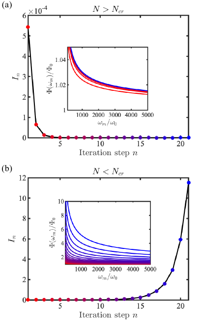
Figure 2: The iterative solution of the gap equation (4) with a constant source term $\Phi(\omega_{m})=\Phi_{0}$ and $\gamma=1/2$. The plots show $I_{n}=\frac{1}{2\pi}\int_{0}^{\infty}\left(\Phi^{n+1}(\omega_{m})-\Phi_{n}(\omega_{m})\right)^{2}d\omega_{m}$. For $N>N_{\text{cr}}$ (a), the iterations converge; for $N<N_{\text{cr}}$ (b), the iterations do not converge. The inserts show how the function $\Phi_{n}(\omega_{m})$ evolves with iterations.

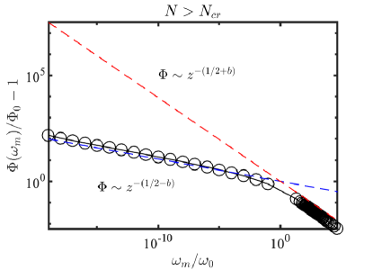
Figure 3: Power-law behavior of the pairing vertex $\Phi(\omega_{m})$ at small frequencies, extracted from the iterative solution for $\gamma=0.5$ and $N=6.5>N_{cr}$. The form of $\Phi(\omega_{m})$ matches the analytical result $\Phi\sim z^{-\gamma(1/2-b)}$ from (19).

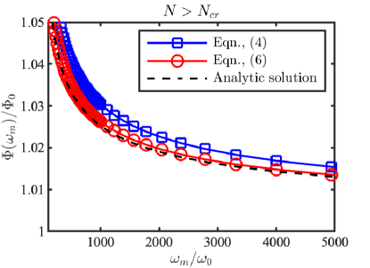
Figure 4: Pairing vertex $\Phi(\omega_{m})$, obtained by solving iteratively the original integral gap equation  (4) (blue line) and the approximate gap equation (6) (red line) for $\gamma=0.5$ and $N=6.5>N_{cr}$.

What happens at smaller $N$, i.e., larger $\lambda=N_{cr}/(4N)$? To answer, we note that our results for $\Phi(z)$ and $\chi_{pp}(z)$ have been obtained by iterations. This procedure is valid as long as the iterations converge. Let’s check the convergence of the series in Eqs. (24) and (28). For this, we need the forms of $D_{n}$ and ${\bar{D}}_{n}$ at large $n$. Using the expressions for Gamma and di-Gamma functions at large argument, we find that $D_{n}$ and ${\bar{D}}_{n}$ decrease at large $n$, but by a power-law rather than exponentially. In explicit form,

$$D_{n}\approx\frac{0.141}{n^{3/2}},~~{\bar{D}}_{n}\approx\frac{0.347}{n^{3/2}}$$ (33)

The $1/n^{3/2}$ dependence ensures that the iterations converge for $\lambda\leq 1$, i.e., for $N\geq N_{cr}$. However, once $N$ gets smaller than $N_{cr}$, the series diverge for both small and large $z$ because $\lambda^{n}=e^{n\log{\lambda}}$ overshoots $1/n^{3/2}$ decay of $D_{n}$ and ${\bar{D}}_{n}$. In Fig. 2(b) we show our numerical results, which confirm that for $\lambda>1$, iteration series diverge for all $z$

To obtain the actual $\chi_{pp}(z)$ for $N<N_{cr}$, we note that its generic form is still a linear combination of $H_{b}(z)$ and $H_{-b}(z)$, but now the argument $b=(1/2)\sqrt{1-\lambda}$ becomes imaginary: $b\to i\tilde{b}$, where

$$\tilde{b}=\frac{1}{2}\sqrt{\lambda-1}$$ (34)

In this situation, $H_{b}(z)$ and $H_{-b}(z)$ become complex conjugated functions $H_{i\tilde{b}}(z)$ and $H_{-i\tilde{b}}(z)$, and both must be kept in (20) to ensure that $\Phi(z)$ is a real function of frequency. A generic real solution of Eq. (6) is

$$\Phi(z)=\Phi(z,\eta)=\Phi_{0}\frac{H_{i\tilde{b}}(z)e^{i\eta}+H_{-i\tilde{b}}(z)e^{-i\eta}}{2\cos{\eta}}$$ (35)

where $\eta$ is arbitrary within $0<\eta<\pi$. There is no condition on $\eta$ as Eq. (36) does not have to match with perturbation theory. Accordingly,

$$\chi_{pp}(z)=\chi_{pp}(z,\eta)=\frac{H_{i\tilde{b}}(z)e^{i\eta}+H_{-i\tilde{b}}(z)e^{-i\eta}}{2\cos{\eta}}$$ (36)

We see that the pairing susceptibility becomes the function not only of $z$ but also of a free parameter $\eta$. To see the outcome, set ${\tilde{b}}$ to be small (i.e., set $N$ to be slightly below $N_{cr}$) and consider large $z$. Using the forms of $H_{\pm i\tilde{b}}(z)$ at small index and large argument, we obtain

$$\chi_{pp}(z,\eta)=1+\frac{1}{4}\frac{\log{z}}{z}+\frac{0.943}{z}\left(1+c\tilde{b}\tan{\eta}\right)$$ (37)

where $c=\pi^{2}/(4*0.943)=2.61$ We see that for any non-zero $\tilde{b}$, there is a range of $\eta\geq\pi/2$, where

$$\pi^{2}{\bar{b}}|\tan{\eta}|>\log{z}$$ (38)

and the pairing susceptibility is negative. This is a clear indication that the system is now below a pairing instability. At the same time, if we choose $\eta=\pi/2$, we find that the pairing susceptibility is infinite. The latter holds for any value of $\tilde{b}$, i.e. for any $N<N_{cr}$. An infinite pairing susceptibility normally implies that the system is right at the onset of a superconducting order. This is very different from BCS case where the pairing susceptibility is a single-valued function, singular at $T_{c}$ and negative at $T<T_{c}$.

This highly unconventional behavior of $\chi_{pp}(z,\eta)$ is fully consistent with the existence of an infinite set of solutions of the non-linear gap equation at $N<N_{cr}$. As we stated in the Introduction, earlier studies have found that in the absence of $\Phi_{0}$, there exists an infinite set of solutions for the pairing vertex $\Phi_{n}(z)$. The solutions are parametrized by $n$ and the overall magnitude of $\Phi_{n}(\omega_{m})$ decreases with increasing $n$. In the limit $n=\infty$, $\Phi_{n}(z)$ is exponentially small and is the solution of the linearized gap equation. In explicit form, $\Phi_{\infty}(z)=iP(H_{i\tilde{b}}(z)-H_{-i\tilde{b}}(z))$, where $P$ is an infinitesimal real number. . Comparing this with our result that the pairing susceptibility depends on a free parameter $\eta$, we see that the existence of a range of $\eta$ where $\chi_{pp}(z,\eta)$ is negative, is consistent with the presence of infinite set of different ordered states, while the fact that $\chi_{pp}(z,\pi/2)$ is infinite is consistent with the still existence of the solution of the linearized gap equation for all $N<N_{cr}$.

We note in passing that there is a certain similarity between the solution of the linearized gap equation at $N<N_{cr}$ in our case and the solution of the relativistic Klein-Gordon/Dirac equation for a heavy atom with an atomic number $Z$ larger than a half of the inverse fine structure constant for a state with the angular momentum $l=0$ (see, e.g., [124, 125] and [126] for a more recent analysis). In both cases the solution (the gap function $\Phi(z)$ in our case and the wave function $\Phi(r)$ for a heavy atom) oscillates at small argument as a function of the logarithm of the argument. Also in both cases a solution is ’weakly” non-normalizable, as it gives rise to logarithmically divergent condensation energy in our case and kinetic energy of an atom. The regularization is provided by non-linearity in our case and a finite atomic size the case of a heavy atom. This analogy clearly deserves further study.

IV Pairing susceptibility for frequency-dependent $\Phi_{0}(\omega_{m})$

For a constant $\Phi_{0}$ as the source term, we found that the pairing susceptibility displays a highly unconventional behavior: it does diverge as $N$ approaches $N_{cr}$ and remains finite and positive at $N=N_{cr}$, but at smaller $N$ becomes a function of a parameter $\eta$ and diverges at $\eta=\pi/2$. We now analyze whether this behavior is specific to a constant $\Phi_{0}$ or persists for frequency-dependent $\Phi_{0}(\omega_{m})$. As before, we will use $z=\omega_{m}^{\gamma}$ instead of $\omega_{m}$. We first consider a particular set of $\Phi_{0}(z)$ and then discuss an arbitrary $\Phi_{0}(z)$. For a set, consider

$$\Phi(z)=\Phi_{0}(1+\epsilon H_{b^{*}}(z))$$ (39)

where $b^{*}$ is positive and real, but different from $b=(1/2)\sqrt{1-N_{cr}/N}$.

We will be searching for the solution of the gap equation (6) in the form

$$\Phi(z)=\Phi_{0}\left(c_{1}H_{b}(z)+c_{2}H_{b^{*}}(z)\right)$$ (40)

substituting this form into the r.h.s of (6) and using (17), we obtain after a simple algebra the set of two equations

$$c_{1}=1-dc_{2},~~c_{2}(1-d)=\epsilon,$$ (41)

where

$$d=\frac{\frac{1}{4}-b^{2}}{\frac{1}{4}-(b^{*})^{2}}$$ (42)

The susceptibility

$$\chi_{pp}(z)=(1+\epsilon)\left(H_{b}+\frac{\epsilon}{1+\epsilon}\frac{H_{b^{*}}(z)-H_{b}(z)}{1-d}\right)$$ (43)

For a generic $b^{*}\neq b$, the susceptibility displays the same behavior as for a constant $\Phi_{0}$, i.e., it remains regular and positive for $N\geq N_{cr}$ and becomes a function of a free parameter $\eta$ at $N<N_{cr}$. The new behavior emerges for a class of $\Phi_{0}(z)$ from (39) with $b^{*}=\alpha b$ and $\alpha$ positive. In this case, $1-d=b^{2}(1-\alpha^{2})/(1/4-\alpha^{2}b^{2})$ and at $H_{b^{*}}(z)-H_{b}(z)=-b(1-\alpha)dH_{b}(z)/db+O(b^{2})$. Expressing $2b=\sqrt{1-\lambda}$, we then obtain at small $b$

$$\chi_{pp}(z)=(1+\epsilon)\left(H_{b}-\frac{1}{2(1+\alpha)}\frac{\left.dH_{b}(z)/db\right|_{b=0}}{\sqrt{1-\lambda}}\right)$$ (44)

We see that for these $\Phi_{0}(z)$, the pairing susceptibility does diverge as $1/\sqrt{N-N_{cr}}$ when $N$ approaches $N_{cr}$ and $\lambda=N_{cr}/N$ approaches $1$. In explicit form $\left.\frac{\partial H_{b}(z)}{\partial b}\right|_{b=0}=G_{2,2}^{2,0}\left(-z\left|\begin{array}[]{cc}0,&1\\ -1/2,&-1/2\\ \end{array}\right.\right)$, where $G^{mn}_{pq}$ is the Meijer $G$ function. It behaves as $\sim\frac{\log z}{\sqrt{z}}$ at $z\rightarrow 0$ and as $\sim\frac{1}{z}$ at $z\rightarrow\infty$.

This result is not surprising as at $N=N_{cr}-0$, the solution of the linearized gap equation without the source term is

$$\Phi(z)=a_{1}H_{0}(z)+b_{2}\left.dH_{b}(z)/db\right|_{b=0}$$ (45)

with arbitrary $a_{1}$ and $a_{2}$. From this perspective, the appearance of $\left.dH_{b}(z)/db\right|_{b=0}$ in (44) with the diverging prefactor at $N\to N_{cr}$, is a clear indication that the system is about to develop spontaneously a non-zero $\Phi(z)$ at $N<N_{cr}$.

These results can be extended to a generic $\Phi_{0}(z)$. We show in the next Section that $\Psi_{\tilde{b}}=iA(H_{i{\tilde{b}}}(z)-H_{-i{\tilde{b}}}(z))$ form a complete set of orthogonal functions which, with a proper normalization factor $A$, satisfy

$$\langle\Psi_{\tilde{b}}|\Psi_{\tilde{b}^{\prime}}\rangle=2\pi\delta(\tilde{b}-\tilde{b^{\prime}}),$$ (46)

An arbitrary $\Phi_{0}(z)$ can then be expressed as

$$\Phi_{0}(z)=\int_{0}^{\infty}d{\tilde{b}}C_{\tilde{b}}\Phi_{\tilde{b}}(z)$$ (47)

Whether the pairing susceptibility remains finite or diverges at $N=N_{cr}$ depends on $C_{0}$. If it vanishes, the pairing susceptibility remains finite at $N=N_{cr}$, while it is non-zero, the susceptibility diverges at $N\to N_{cr}$ as $1/\sqrt{N-N_{cr}}$.

V Physical reasoning

We now go back to the issue about the number of solutions of the gap equation with the external source $\Phi_{0}(z)$. We recall that Eq. (7) has two linearly independent solutions for any $N$, see (19), yet only one solution is reproduced by iterations at $N>N_{cr}$. A natural question then is whether there a physical reasoning for choosing the one-component solution selected by the iterations and not a general two-component solution. In this section we give such a reasoning using the analogy between our gap equation and Schrodinger equation in quantum mechanics.

To do this, we go back to the basics of Eliashberg theory and recall the requirement that the condensation energy $E[\Phi(\omega_{m})]$ for a given $\Phi(\omega_{m})$ must be finite, otherwise the probability to find the state with this $\Phi(\omega_{m})$ vanishes. For infinitesimally small $\Phi(\omega_{m})$, which we consider in this paper, the condensation energy $E_{c}$ is quadratic in $\Phi(\omega_{m})$ and is given by

$$E_{c}=A\int_{0}^{\infty}\frac{\Phi^{2}(\omega_{m})d\omega_{m}}{|\omega_{m}|^{1-\gamma}(1+|\omega_{m}|^{\gamma})}.$$ (48)

where $A$ is a finite overall factor.

In analogy with quantum mechanics, the gap equation can be re-expressed as the effective Schroedinger-type equation $\Phi(\omega_{m})=\hat{L}\Phi(\omega_{m})+\Phi_{0}(\omega_{m})$ with the linear operator

$$\hat{L}\Phi(\omega_{m})=\int\frac{d\omega^{{}^{\prime}}_{m}\Phi(\omega^{{}^{\prime}}_{m})}{|\omega^{{}^{\prime}}_{m}|^{1-\gamma}|\omega_{m}-\omega^{{}^{\prime}}_{m}|^{\gamma}}\frac{1}{1+|\omega^{{}^{\prime}}_{m}|^{\gamma}}$$ (49)

Then $\Phi(\omega_{m})$ can be viewed as a (real) wavefunction, and the condensation energy, or, equivalently, the scalar product in the space of wavefunctions $\langle\Phi|\Psi\rangle$ can be viewed as the norm. The scalar product is defined as

$$\langle\Phi|\Psi\rangle=\int_{0}^{\infty}\frac{\Phi(\omega_{m})\Psi(\omega_{m})d\omega_{m}}{|\omega_{m}|^{1-\gamma}(1+|\omega_{m}|^{\gamma})}.$$ (50)

and the condensation energy is

$$E_{c}=A\langle\Phi|\Phi\rangle$$ (51)

One can immediately check that for the scalar product defined in (50) $\langle\Phi|\hat{L}\Psi\rangle=\langle\hat{L}\Phi|\Psi\rangle$, i,e., the linear operator ${\hat{L}}$ is Hermitian, as the physical operator should be. Physically meaningful $\Phi(\omega_{m})$ then should have a finite norm. For the truncated integral equation (7) we introduce $z=\omega^{\gamma}_{m}$ and

$$\hat{\Pi}\Phi(z)=\frac{1}{z}\int_{0}^{z}\frac{\Phi(x)dx}{1+x}+\int_{z}^{\infty}\frac{\Phi(x)dx}{x(1+x)}$$ (52)

and re-express (7) as

$$\Phi(z)=\left(\frac{1}{4}-b^{2}\right)\hat{\Pi}\Phi(z)+\Phi_{0}(z)$$ (53)

One can verify that $\hat{\Pi}$ is also Hermitian for the scalar product defined in (50), so physically meaningful $\Phi(z)$ should have a finite norm.

For $\Phi_{0}(z)=\Phi_{0}$, there are two eigenfunctions $\Phi_{1}(z)=H_{b}(z)$ and $\Phi_{2}(z)=H_{-b}(z)$, see (13). Substituting both into (51) and analyzing the behavior at $z\rightarrow 0$, we see that $H_{b}(z)$ has a finite norm, while the norm of $H_{-b}(z)$ diverges. Hence, only $H_{b}(z)$ is physically meaningful. This is physical justification for choosing $\Phi(z)=\Phi_{0}H_{b}(z)$ based on the iteration procedure.

We can analyze the equation (53) further. Let’s set $\Phi_{0}(z)=0$. The gap equation becomes

$$\hat{\Pi}\Phi_{\epsilon}=\epsilon_{b}\Phi_{\epsilon}$$ (54)

where $\epsilon_{b}=\left(1/4-b^{2}\right)^{-1}$. This is an equation for eigenvalues/eigenfunctions of the operator $\hat{\Pi}$ in the space of wavefunctions with the norm defined in (50). As $\hat{\Pi}$ is Hermitian, all eigenvalues are real. The solution of (54) is formally $\Phi(z)\propto\left(H_{b}(z)-H_{-b}(z)\right)$ for any $b$, but the normalizable solution appears only at $N<N_{cr}$, when $b=i\tilde{b}$ is imaginary. Then the eigenvalue is $\epsilon_{b}=\left(1/4+\tilde{b}^{2}\right)^{-1}$ and the physically meaningful eigenfunction is

$$\Phi_{\tilde{b}}=iA\left(H_{i\tilde{b}}(z)-H_{-i\tilde{b}}(z)\right),$$ (55)

where $A$ is the normalization factor.

We see that the operator $\hat{\Pi}$ has a continuous spectrum $\epsilon\in[0,1/4]$. The eigenfunctions must then be normalized by

$$\langle\Phi_{\tilde{b}}|\Phi_{\tilde{b}^{\prime}}\rangle=2\pi\delta(\tilde{b}-\tilde{b^{\prime}})$$ (56)

We can then introduce the Green’s function $G(z,z^{\prime})$ as

$$G_{b}(z,z^{\prime})=\int_{0}^{\infty}\frac{\Phi_{\tilde{b}}(z)\Phi_{\tilde{b}}(z^{\prime})}{\left(\frac{1}{4}-b^{2}\right)^{-1}-\epsilon_{\tilde{b}}}\frac{d\tilde{b}}{2\pi}.$$ (57)

and write the solution of the gap equation (7) with the source term $\Phi_{0}(z)$ as

$$\Phi(z)=\left(\frac{1}{4}-b^{2}\right)^{-1}\int_{0}^{\infty}G_{b}(z,z^{\prime})\Phi_{0}(z^{\prime})\frac{dz^{\prime}}{1+z^{\prime}}$$ (58)

For $b>0$ ($N>N_{cr}$) , $G_{b}(z,z^{\prime})$ is regular and $\Phi(z)$ is single-valued. The susceptibility $\chi_{pp}(z)$ is a regular (non-divergent) function of $z$.

For $b=i\tilde{b}$ ($N<N_{cr}$), the integral in (57) diverges. The solution then becomes

$$\Phi(z)=\Phi_{p}(z)+{\bar{\eta}}\Phi_{\tilde{b}}$$ (59)

where $\Phi_{p}(z)$ is a particular normalizable solution of (7) and ${\bar{\eta}}$ is an arbitrary (real) number. The pairing susceptibility then becomes a function of a free running parameter ${\bar{\eta}}$, in agreement with the analysis in the previous Section.

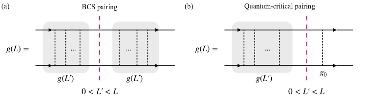
Figure 5: An illustration of the structure of the one-loop RG equation for the 4-fermion interaction vertex for (a) BCS pairing in a Fermi liquid and (b) quantum-critical pairing out of a non-Fermi liquid.

VI Conclusions

In this paper we analyzed the dynamical pairing susceptibility $\chi_{pp}(\omega_{m})$ (the ratio of the fully dressed dynamical pairing vertex $\Phi(\omega_{m})$ and the bare $\Phi_{0}(\omega_{m})$) at zero temperature in a quantum-critical metal, where superconductivity emerges out of a non-Fermi liquid ground state once the pairing interaction exceeds a certain threshold. We showed that this susceptibility is qualitatively different from that for superconductivity emerging out of a Fermi liquid. There, the pairing susceptibility is positive above the transition, diverges at the transition, and becomes negative below it. In the quantum-critical case, we found for a static $\Phi_{0}$ that $\chi_{pp}(\omega_{m})$ remains positive and non-singular all the way up to a pairing instability, and becomes a function of both $\omega_{m}$ and a free parameter $\eta$ immediately below the instability. We argued that this highly unconventional behavior of $\chi_{pp}(\omega_{m})$ reflects a multi-critical nature of a $T=0$ onset point of superconductivity in a quantum-critical metal when an infinite number of superconducting states emerges simultaneously with different amplitudes of the order parameter, down to an infinitesimally small one. We discussed how the pairing susceptibility behaves for a generic dynamical $\Phi_{0}(\omega_{m})$ and established the conditions when $\chi_{pp}(\omega_{m})$ remains finite at the critical point and when it diverges at criticality. We also presented physical reasoning based on the analogy between the gap equation at the critical point and Schrodinger-type equation in quantum mechanics.

Appendix A Pairing susceptibility in the renormalization group treatment

In this Appendix we show how the pairing susceptibility can be obtained within the renormalization group (RG) formalism. For this, one has to analyze ladder renormalizations of the 4-fermion pairing interaction.

In BCS theory, the bare value of the pairing interaction is $g_{0}=\lambda^{*}/N$, and the running one, $g(L)$, is a function of $L=\log{\Lambda/T}$. The one-loop RG equation is obtained by (i) selecting a cross-section in the ladder series, in which intermediate $L^{\prime}$ are set to be larger than in other cross-sections, (ii) expressing the momentum/frequency integral in this cross-section as $\int_{0}^{L}dL^{\prime}$, and (iii) summing up the renormalizations of $g$ on both sides of this cross-section over intermediate $L^{\prime\prime}$ up to $L^{\prime}$ (Fig. 5(a)). Each of such renormalizations yields $g(L^{\prime})$, and the full ladder renormalization is expressed as

$$g(L)=\int_{0}^{L}dL^{\prime}g^{2}(L^{\prime}),~~{\text{i}.e}~~\frac{dg(L)}{dL}=g^{2}(L)$$ (60)

Solving this equation one obtains for the susceptibility $\chi_{pp}(L)=g(L)/g_{0}$

$$\chi_{pp}(L)=\frac{1}{1-g_{0}L}=\frac{1}{1-\left(\frac{\lambda^{*}}{N}\right)\log{\frac{\Lambda}{T}}}$$ (61)

which is the same as $\chi_{pp}$ in (10).

For quantum-critical pairing, the RG analysis is applied most naturally to 4-fermion vertex with small incoming frequencies $(\omega_{m},-\omega_{m})$ and much larger outgoing frequencies of order one (all frequencies in unites of $\omega_{0}$). The bare coupling is $g_{0}=(1-\gamma)/N$ and the running $g(L)$ is a function of $L=\log(1/|\omega_{m}|)$. The one-loop RG equation is again obtained by choosing the cross-section with the largest $L^{\prime}$. The momentum/frequency integral in this cross-section yields $\int_{0}^{L}dL^{\prime}$, as in the BCS case. The difference with BCS comes about because this cross-section is now at the boundary rather than in the middle (Fig. 5(b)), as one can explicitly verify [10]. As a result, the renormalizations in other cross-sections yield $g_{0}g(L)$ rather than $g^{2}(L)$. We then obtain

$$g(L)=g_{0}\int_{0}^{L}dL^{\prime}g(L^{\prime}),~~{\text{i}.e}~~\frac{dg(L)}{dL}=g_{0}g(L)$$ (62)

Solving this equation, one obtains the susceptibility $\chi_{pp}(L)=g(L)/g_{0}$

$$\chi_{pp}(L)=e^{g_{0}L}=\frac{1}{|\omega_{m}|^{\frac{1-\gamma}{N}}},$$ (63)

which is the same as (12).

References

- Lee [1989] P. A. Lee, Gauge field, aharonov-bohm flux, and high- superconductivity, Phys. Rev. Lett. 63, 680 (1989).
- Blok and Monien [1993] B. Blok and H. Monien, Gauge theories of high- superconductors, Phys. Rev. B 47, 3454 (1993).
- Nayak and Wilczek [1994] C. Nayak and F. Wilczek, Non-fermi liquid fixed point in 2 + 1 dimensions, Nuclear Physics B 417, 359 (1994).
- Altshuler et al. [1994] B. L. Altshuler, L. B. Ioffe, and A. J. Millis, Low-energy properties of fermions with singular interactions, Phys. Rev. B 50, 14048 (1994).
- Kim et al. [1994] Y. B. Kim, A. Furusaki, X.-G. Wen, and P. A. Lee, Gauge-invariant response functions of fermions coupled to a gauge field, Phys. Rev. B 50, 17917 (1994).
- You et al. [2016] Y. You, G. Y. Cho, and E. Fradkin, Nematic quantum phase transition of composite fermi liquids in half-filled landau levels and their geometric response, Phys. Rev. B 93, 205401 (2016).
- Millis [1992] A. J. Millis, Nearly antiferromagnetic fermi liquids: An analytic eliashberg approach, Phys. Rev. B 45, 13047 (1992).
- Altshuler et al. [1995] B. L. Altshuler, L. B. Ioffe, A. I. Larkin, and A. J. Millis, Spin-density-wave transition in a two-dimensional spin liquid, Phys. Rev. B 52, 4607 (1995).
- Sachdev et al. [1995] S. Sachdev, A. V. Chubukov, and A. Sokol, Crossover and scaling in a nearly antiferromagnetic fermi liquid in two dimensions, Phys. Rev. B 51, 14874 (1995).
- Abanov et al. [2001a] A. Abanov, A. V. Chubukov, and A. M. Finkel’stein, Coherent vs . incoherent pairing in 2D systems near magnetic instability, EPL (Europhysics Letters) 54, 488 (2001a).
- Abanov et al. [2003] A. Abanov, A. V. Chubukov, and J. Schmalian, Quantum-critical theory of the spin-fermion model and its application to cuprates: Normal state analysis, Advances in Physics 52, 119 (2003).
- Abanov and Chubukov [1999] A. Abanov and A. V. Chubukov, A relation between the resonance neutron peak and arpes data in cuprates, Phys. Rev. Lett. 83, 1652 (1999).
- Abanov et al. [2001b] A. Abanov, A. V. Chubukov, and J. Schmalian, Fingerprints of spin mediated pairing in cuprates, Journal of Electron spectroscopy and related phenomena 117, 129 (2001b).
- Abanov et al. [2008] A. Abanov, A. V. Chubukov, and M. R. Norman, Gap anisotropy and universal pairing scale in a spin-fluctuation model of cuprate superconductors, Phys. Rev. B 78, 220507 (2008).
- Sachdev et al. [2009] S. Sachdev, M. A. Metlitski, Y. Qi, and C. Xu, Fluctuating spin density waves in metals, Phys. Rev. B 80, 155129 (2009).
- Moon and Sachdev [2009] E. G. Moon and S. Sachdev, Competition between spin density wave order and superconductivity in the underdoped cuprates, Phys. Rev. B 80, 035117 (2009).
- Sachdev et al. [2019] S. Sachdev, H. D. Scammell, M. S. Scheurer, and G. Tarnopolsky, Gauge theory for the cuprates near optimal doping, Phys. Rev. B 99, 054516 (2019).
- Vojta and Sachdev [1999] M. Vojta and S. Sachdev, Charge order, superconductivity, and a global phase diagram of doped antiferromagnets, Phys. Rev. Lett. 83, 3916 (1999).
- Li et al. [2023] C. Li, S. Sachdev, and D. G. Joshi, Superconductivity of non-fermi liquids described by sachdev-ye-kitaev models, Phys. Rev. Res. 5, 013045 (2023).
- Wang and Chubukov [2013] Y. Wang and A. V. Chubukov, Superconductivity at the onset of spin-density-wave order in a metal, Phys. Rev. Lett. 110, 127001 (2013).
- Efetov et al. [2013] K. B. Efetov, H. Meier, and C. Pepin, Pseudogap state near a quantum critical point, Nature Physics 9, 442 (2013).
- Meier et al. [2014] H. Meier, C. Pépin, M. Einenkel, and K. B. Efetov, Cascade of phase transitions in the vicinity of a quantum critical point, Phys. Rev. B 89, 195115 (2014).
- Efetov [2015] K. B. Efetov, Quantum criticality in two dimensions and marginal fermi liquid, Phys. Rev. B 91, 045110 (2015).
- Benlagra et al. [2011] A. Benlagra, K. Kim, and C. Pépin, The luttinger–ward functional approach in the eliashberg framework: a systematic derivation of scaling for thermodynamics near the quantum critical point, Journal of Physics: Condensed Matter 23, 145601 (2011).
- Metlitski and Sachdev [2010a] M. A. Metlitski and S. Sachdev, Quantum phase transitions of metals in two spatial dimensions. i. ising-nematic order, Physical Review B 82, 075127 (2010a).
- Metlitski and Sachdev [2010b] M. A. Metlitski and S. Sachdev, Quantum phase transitions of metals in two spatial dimensions. ii. spin density wave order, Physical Review B 82, 075128 (2010b).
- Hartnoll et al. [2011] S. A. Hartnoll, D. M. Hofman, M. A. Metlitski, and S. Sachdev, Quantum critical response at the onset of spin-density-wave order in two-dimensional metals, Phys. Rev. B 84, 125115 (2011).
- Metlitski et al. [2015] M. A. Metlitski, D. F. Mross, S. Sachdev, and T. Senthil, Cooper pairing in non-fermi liquids, Phys. Rev. B 91, 115111 (2015).
- Dalidovich and Lee [2013] D. Dalidovich and S.-S. Lee, Perturbative non-fermi liquids from dimensional regularization, Phys. Rev. B 88, 245106 (2013).
- Lee [2018] S.-S. Lee, Recent developments in non-fermi liquid theory, Annual Review of Condensed Matter Physics 9, 227 (2018).
- Bauer and Sachdev [2015] J. Bauer and S. Sachdev, Real-space eliashberg approach to charge order of electrons coupled to dynamic antiferromagnetic fluctuations, Phys. Rev. B 92, 085134 (2015).
- Castellani et al. [1995] C. Castellani, C. Di Castro, and M. Grilli, Singular quasiparticle scattering in the proximity of charge instabilities, Phys. Rev. Lett. 75, 4650 (1995).
- Perali et al. [1996] A. Perali, C. Castellani, C. Di Castro, and M. Grilli, d-wave superconductivity near charge instabilities, Phys. Rev. B 54, 16216 (1996).
- Andergassen et al. [2001] S. Andergassen, S. Caprara, C. Di Castro, and M. Grilli, Anomalous isotopic effect near the charge-ordering quantum criticality, Phys. Rev. Lett. 87, 056401 (2001).
- Wang and Chubukov [2015] Y. Wang and A. V. Chubukov, Enhancement of superconductivity at the onset of charge-density-wave order in a metal, Phys. Rev. B 92, 125108 (2015).
- Chowdhury and Sachdev [2014a] D. Chowdhury and S. Sachdev, Feedback of superconducting fluctuations on charge order in the underdoped cuprates, Phys. Rev. B 90, 134516 (2014a).
- Chowdhury and Sachdev [2014b] D. Chowdhury and S. Sachdev, Density-wave instabilities of fractionalized fermi liquids, Phys. Rev. B 90, 245136 (2014b).
- Gerlach et al. [2017] M. H. Gerlach, Y. Schattner, E. Berg, and S. Trebst, Quantum critical properties of a metallic spin-density-wave transition, Phys. Rev. B 95, 035124 (2017).
- Schattner et al. [2016] Y. Schattner, S. Lederer, S. A. Kivelson, and E. Berg, Ising nematic quantum critical point in a metal: A monte carlo study, Phys. Rev. X 6, 031028 (2016).
- Wang et al. [2017a] X. Wang, Y. Schattner, E. Berg, and R. M. Fernandes, Superconductivity mediated by quantum critical antiferromagnetic fluctuations: The rise and fall of hot spots, Phys. Rev. B 95, 174520 (2017a).
- Xu et al. [2017] X. Y. Xu, K. Sun, Y. Schattner, E. Berg, and Z. Y. Meng, Non-fermi liquid at () ferromagnetic quantum critical point, Phys. Rev. X 7, 031058 (2017).
- Berg et al. [2019] E. Berg, S. Lederer, Y. Schattner, and S. Trebst, Monte carlo studies of quantum critical metals, Annual Review of Condensed Matter Physics 10, 63 (2019).
- Jiang et al. [2022] W. Jiang, Y. Liu, A. Klein, Y. Wang, K. Sun, A. V. Chubukov, and Z. Y. Meng, Monte carlo study of the pseudogap and superconductivity emerging from quantum magnetic fluctuations, Nature Communications 13, 2655 (2022).
- Shibauchi et al. [2014] T. Shibauchi, A. Carrington, and Y. Matsuda, Quantum critical point lying beneath the superconducting dome in iron-pnictides, Annual Review of Condensed Matter Physics 5, 113 (2014).
- Löhneysen et al. [2007] H. v. Löhneysen, A. Rosch, M. Vojta, and P. Wölfle, Fermi-liquid instabilities at magnetic quantum phase transitions, Rev. Mod. Phys. 79, 1015 (2007).
- Khodas et al. [2010] M. Khodas, H. B. Yang, J. Rameau, P. D. Johnson, A. M. Tsvelik, and T. M. Rice, Analysis of the quasiparticle spectral function in the underdoped cuprates, ArXiv:1007.4837 (2010).
- Tsvelik [2017] A. M. Tsvelik, Ladder physics in the spin fermion model, Phys. Rev. B 95, 201112 (2017).
- Konik et al. [2010] R. M. Konik, T. M. Rice, and A. M. Tsvelik, Superconductivity generated by coupling to a cooperon in a two-dimensional array of four-leg hubbard ladders, Phys. Rev. B 82, 054501 (2010).
- Khodas and Tsvelik [2010] M. Khodas and A. M. Tsvelik, Influence of thermal phase fluctuations on the spectral function for a two-dimensional -wave superconductor, Phys. Rev. B 81, 094514 (2010).
- Chubukov and Tsvelik [2007] A. V. Chubukov and A. M. Tsvelik, Spin-liquid model of the sharp drop in resistivity in superconducting , Phys. Rev. B 76, 100509 (2007).
- Metzner et al. [2003] W. Metzner, D. Rohe, and S. Andergassen, Soft fermi surfaces and breakdown of fermi-liquid behavior, Phys. Rev. Lett. 91, 066402 (2003).
- Dell’Anna and Metzner [2006] L. Dell’Anna and W. Metzner, Fermi surface fluctuations and single electron excitations near pomeranchuk instability in two dimensions, Phys. Rev. B 73, 045127 (2006).
- Vilardi et al. [2018] D. Vilardi, C. Taranto, and W. Metzner, Antiferromagnetic and d-wave pairing correlations in the strongly interacting two-dimensional hubbard model from the functional renormalization group, arXiv:1810.02290 and references therein (2018).
- Holder and Metzner [2015] T. Holder and W. Metzner, Fermion loops and improved power-counting in two-dimensional critical metals with singular forward scattering, Phys. Rev. B 92, 245128 (2015).
- Yamase et al. [2016] H. Yamase, A. Eberlein, and W. Metzner, Coexistence of incommensurate magnetism and superconductivity in the two-dimensional hubbard model, Phys. Rev. Lett. 116, 096402 (2016).
- Sordi et al. [2012] G. Sordi, P. Simon, K. Haule, and A.-M. S. Tremblay, Strong coupling superconductivity, pseudogap, and mott transition, Phys. Rev. Lett. 108, 216401 (2012).
- She and Zaanen [2009] J.-H. She and J. Zaanen, Bcs superconductivity in quantum critical metals, Phys. Rev. B 80, 184518 (2009).
- Yang et al. [2011] S.-X. Yang, H. Fotso, S.-Q. Su, D. Galanakis, E. Khatami, J.-H. She, J. Moreno, J. Zaanen, and M. Jarrell, Proximity of the superconducting dome and the quantum critical point in the two-dimensional hubbard model, Phys. Rev. Lett. 106, 047004 (2011).
- Chubukov and Wölfle [2014] A. V. Chubukov and P. Wölfle, Quasiparticle interaction function in a two-dimensional fermi liquid near an antiferromagnetic critical point, Phys. Rev. B 89, 045108 (2014).
- Varma [2016] C. M. Varma, Quantum-critical fluctuations in 2d metals: strange metals and superconductivity in antiferromagnets and in cuprates, Reports on Progress in Physics 79, 082501 (2016).
- Georges et al. [2013] A. Georges, L. d. Medici, and J. Mravlje, Strong correlations from hund’s coupling, Annu. Rev. Condens. Matter Phys. 4, 137 (2013).
- Lee et al. [2018] T.-H. Lee, A. Chubukov, H. Miao, and G. Kotliar, Pairing mechanism in hund’s metal superconductors and the universality of the superconducting gap to critical temperature ratio, Phys. Rev. Lett. 121, 187003 (2018).
- Wu et al. [2019] Y.-M. Wu, A. Abanov, and A. V. Chubukov, Pairing in quantum critical systems: Transition temperature, pairing gap, and their ratio, Phys. Rev. B 99, 014502 (2019).
- Klein et al. [2020] A. Klein, A. V. Chubukov, Y. Schattner, and E. Berg, Normal state properties of quantum critical metals at finite temperature, Phys. Rev. X 10, 031053 (2020).
- Klein et al. [2019] A. Klein, Y.-M. Wu, and A. V. Chubukov, Multiple intertwined pairing states and temperature-sensitive gap anisotropy for superconductivity at a nematic quantum-critical point, npj Quantum Materials 4, 55 (2019).
- Klein and Chubukov [2018] A. Klein and A. Chubukov, Superconductivity near a nematic quantum critical point: Interplay between hot and lukewarm regions, Phys. Rev. B 98, 220501 (2018).
- Liu et al. [2022] Y. Liu, W. Jiang, A. Klein, Y. Wang, K. Sun, A. V. Chubukov, and Z. Y. Meng, Dynamical exponent of a quantum critical itinerant ferromagnet: A monte carlo study, Phys. Rev. B 105, L041111 (2022).
- Kumar et al. [2024] A. Kumar, A. S. Patri, and T. Senthil, Unconventional superconductivity mediated by exciton density wave fluctuations (2024), arXiv:2410.09148 [cond-mat.str-el] .
- Nosov et al. [2023] P. A. Nosov, I. S. Burmistrov, and S. Raghu, Interplay of superconductivity and localization near a two-dimensional ferromagnetic quantum critical point, Phys. Rev. B 107, 144508 (2023).
- Wu et al. [2023] T. C. Wu, P. A. Lee, and M. S. Foster, Enhancement of superconductivity in a dirty marginal fermi liquid, Phys. Rev. B 108, 214506 (2023).
- Scalapino [1969] D. J. Scalapino, The electron-phonon interaction and strong-coupling superconductors, Superconductivity, Ed. R.D. Parks (Dekker, New York, 1969) p 449 (1969).
- Monthoux et al. [2007] P. Monthoux, D. Pines, and G. G. Lonzarich, Superconductivity without phonons, Nature 450, 1177 (2007).
- Marsiglio and Carbotte [1991] F. Marsiglio and J. P. Carbotte, Gap function and density of states in the strong-coupling limit for an electron-boson system, Phys. Rev. B 43, 5355 (1991), for more recent results see F. Marsiglio and J.P. Carbotte, “Electron-Phonon Superconductivity”, in “The Physics of Conventional and Unconventional Superconductors”, Bennemann and Ketterson eds., Springer-Verlag, (2006) and references therein; F. Marsiglio, Annals of Physics 417, 168102-1-23 (2020).
- Allen and Dynes [1975] P. B. Allen and R. C. Dynes, Transition temperature of strong-coupled superconductors reanalyzed, Phys. Rev. B 12, 905 (1975).
- Combescot [1995] R. Combescot, Strong-coupling limit of eliashberg theory, Phys. Rev. B 51, 11625 (1995).
- Mirabi et al. [2020] S. Mirabi, R. Boyack, and F. Marsiglio, Thermodynamics of eliashberg theory in the weak-coupling limit, Phys. Rev. B 102, 214505 (2020).
- Protter et al. [2021] M. Protter, R. Boyack, and F. Marsiglio, Functional-integral approach to gaussian fluctuations in eliashberg theory, Phys. Rev. B 104, 014513 (2021).
- Esterlis et al. [2018] I. Esterlis, B. Nosarzewski, E. W. Huang, B. Moritz, T. P. Devereaux, D. J. Scalapino, and S. A. Kivelson, Breakdown of the migdal-eliashberg theory: A determinant quantum monte carlo study, Phys. Rev. B 97, 140501 (2018).
- Chubukov et al. [2020a] A. V. Chubukov, A. Abanov, I. Esterlis, and S. A. Kivelson, Eliashberg theory of phonon-mediated superconductivity – when it is valid and how it breaks down, Annals of Physics 417, 168190 (2020a).
- Zhang et al. [2023a] C. Zhang, J. Sous, D. R. Reichman, M. Berciu, A. J. Millis, N. V. Prokof’ev, and B. V. Svistunov, Bipolaronic high-temperature superconductivity, Phys. Rev. X 13, 011010 (2023a).
- Secchi et al. [2020] A. Secchi, M. Polini, and M. I. Katsnelson, Phonon-mediated superconductivity in strongly correlated electron systems: A luttinger–ward functional approach, Annals of Physics 417, 168100 (2020).
- Yuzbashyan et al. [2022] E. A. Yuzbashyan, M. K.-H. Kiessling, and B. L. Altshuler, Superconductivity near a quantum critical point in the extreme retardation regime, Phys. Rev. B 106, 064502 (2022).
- Yuzbashyan and Altshuler [2022a] E. A. Yuzbashyan and B. L. Altshuler, Migdal-eliashberg theory as a classical spin chain, Phys. Rev. B 106, 014512 (2022a).
- Yuzbashyan and Altshuler [2022b] E. A. Yuzbashyan and B. L. Altshuler, Breakdown of the migdal-eliashberg theory and a theory of lattice-fermionic superfluidity, Phys. Rev. B 106, 054518 (2022b).
- Yuzbashyan et al. [2024] E. A. Yuzbashyan, B. L. Altshuler, and A. Patra, Instability of metals with respect to strong electron-phonon interaction (2024), arXiv:2409.19562 [cond-mat.str-el] .
- Semenok et al. [2024] D. V. Semenok, B. L. Altshuler, and E. A. Yuzbashyan, Fundamental limits on the electron-phonon coupling and superconducting (2024), arXiv:2407.12922 [cond-mat.supr-con] .
- Kiessling et al. [2024a] M. Kiessling, B. Altshuler, and E. Yuzbashyan, Bounds on in the eliashberg theory of superconductivity. ii: Dispersive phonons (2024a), arXiv:2409.00532 [math-ph] .
- Kiessling et al. [2024b] M. Kiessling, B. Altshuler, and E. Yuzbashyan, Bounds on in the eliashberg theory of superconductivity. iii: Einstein phonons (2024b), arXiv:2409.02121 [cond-mat.supr-con] .
- Zhang et al. [2022] S.-S. Zhang, Y.-M. Wu, A. Abanov, and A. V. Chubukov, Superconductivity out of a non-fermi liquid: Free energy analysis, Phys. Rev. B 106, 144513 (2022).
- Zhang et al. [2023b] S.-S. Zhang, E. Berg, and A. V. Chubukov, Free energy and specific heat near a quantum critical point of a metal, Phys. Rev. B 107, 144507 (2023b).
- Patel and Sachdev [2019] A. A. Patel and S. Sachdev, Theory of a planckian metal, Phys. Rev. Lett. 123, 066601 (2019).
- Esterlis and Schmalian [2019] I. Esterlis and J. Schmalian, Cooper pairing of incoherent electrons: An electron-phonon version of the sachdev-ye-kitaev model, Phys. Rev. B 100, 115132 (2019).
- Wang [2020] Y. Wang, Solvable strong-coupling quantum-dot model with a non-fermi-liquid pairing transition, Phys. Rev. Lett. 124, 017002 (2020).
- Hauck et al. [2020] D. Hauck, M. J. Klug, I. Esterlis, and J. Schmalian, Eliashberg equations for an electron-phonon version of the sachdev-ye-kitaev model: Pair breaking in non-fermi liquid superconductors, Annals of Physics 417, 168120 (2020).
- Chowdhury and Berg [2020] D. Chowdhury and E. Berg, Intrinsic superconducting instabilities of a solvable model for an incoherent metal, Phys. Rev. Research 2, 013301 (2020).
- Classen and Chubukov [2021] L. Classen and A. Chubukov, Superconductivity of incoherent electrons in the yukawa sachdev-ye-kitaev model, Phys. Rev. B 104, 125120 (2021).
- Classen and Betouras [2024] L. Classen and J. J. Betouras, High-order van hove singularities and their connection to flat bands, Annual Review of Condensed Matter Physics (2024).
- Shtyk et al. [2017] A. Shtyk, G. Goldstein, and C. Chamon, Electrons at the monkey saddle: A multicritical lifshitz point, Phys. Rev. B 95, 035137 (2017).
- Ojajärvi et al. [2024] R. Ojajärvi, A. V. Chubukov, Y.-C. Lee, M. Garst, and J. Schmalian, Pairing at a single van hove point (2024), arXiv:2408.05572 [cond-mat.supr-con] .
- Raghu et al. [2015] S. Raghu, G. Torroba, and H. Wang, Metallic quantum critical points with finite bcs couplings, Phys. Rev. B 92, 205104 (2015).
- Fitzpatrick et al. [2013] A. L. Fitzpatrick, S. Kachru, J. Kaplan, and S. Raghu, Non-fermi-liquid fixed point in a wilsonian theory of quantum critical metals, Phys. Rev. B 88, 125116 (2013).
- Fitzpatrick et al. [2014] A. L. Fitzpatrick, S. Kachru, J. Kaplan, and S. Raghu, Non-fermi-liquid behavior of large- quantum critical metals, Phys. Rev. B 89, 165114 (2014).
- Fitzpatrick et al. [2015] A. L. Fitzpatrick, S. Kachru, J. Kaplan, S. Raghu, G. Torroba, and H. Wang, Enhanced pairing of quantum critical metals near , Phys. Rev. B 92, 045118 (2015).
- Moon and Chubukov [2010] E.-G. Moon and A. Chubukov, Quantum-critical pairing with varying exponents, Journal of Low Temperature Physics 161, 263 (2010).
- Wang et al. [2016] Y. Wang, A. Abanov, B. L. Altshuler, E. A. Yuzbashyan, and A. V. Chubukov, Superconductivity near a quantum-critical point: The special role of the first matsubara frequency, Phys. Rev. Lett. 117, 157001 (2016).
- Abanov and Chubukov [2020] A. Abanov and A. V. Chubukov, Interplay between superconductivity and non-fermi liquid at a quantum critical point in a metal. i. the model and its phase diagram at : The case , Phys. Rev. B 102, 024524 (2020).
- Wu et al. [2020a] Y.-M. Wu, A. Abanov, Y. Wang, and A. V. Chubukov, Interplay between superconductivity and non-fermi liquid at a quantum critical point in a metal. ii. the model at a finite for , Phys. Rev. B 102, 024525 (2020a).
- Wu et al. [2020b] Y.-M. Wu, A. Abanov, and A. V. Chubukov, Interplay between superconductivity and non-fermi liquid behavior at a quantum critical point in a metal. iii. the model and its phase diagram across , Phys. Rev. B 102, 094516 (2020b).
- Wu et al. [2021a] Y.-M. Wu, S.-S. Zhang, A. Abanov, and A. V. Chubukov, Interplay between superconductivity and non-fermi liquid at a quantum critical point in a metal. iv. the model and its phase diagram at , Phys. Rev. B 103, 024522 (2021a).
- Wu et al. [2021b] Y.-M. Wu, S.-S. Zhang, A. Abanov, and A. V. Chubukov, Interplay between superconductivity and non-fermi liquid behavior at a quantum-critical point in a metal. v. the model and its phase diagram: The case , Phys. Rev. B 103, 184508 (2021b).
- Zhang et al. [2021] S.-S. Zhang, Y.-M. Wu, A. Abanov, and A. V. Chubukov, Interplay between superconductivity and non-fermi liquid at a quantum critical point in a metal. vi. the model and its phase diagram at , Phys. Rev. B 104, 144509 (2021).
- Wu et al. [2022] Y.-M. Wu, S.-S. Zhang, A. Abanov, and A. V. Chubukov, Odd frequency pairing in a quantum critical metal, Phys. Rev. B 106, 094506 (2022).
- Chubukov and Abanov [2021] A. V. Chubukov and A. Abanov, Pairing by a dynamical interaction in a metal, Journal of Experimental and Theoretical Physics 132, 606 (2021).
- Kiessling et al. [2024c] M. Kiessling, B. Altshuler, and E. Yuzbashyan, Bounds on in the eliashberg theory of superconductivity. i: The -model (2024c), arXiv:2409.00533 [math-ph] .
- Khveshchenko and Shively [2006] D. V. Khveshchenko and W. F. Shively, Excitonic pairing between nodal fermions, Phys. Rev. B 73, 115104 (2006).
- Chubukov et al. [2020b] A. V. Chubukov, A. Abanov, Y. Wang, and Y.-M. Wu, The interplay between superconductivity and non-fermi liquid at a quantum-critical point in a metal, Annals of Physics 417, 168142 (2020b).
- Wang et al. [2017b] H. Wang, S. Raghu, and G. Torroba, Non-fermi-liquid superconductivity: Eliashberg approach versus the renormalization group, Phys. Rev. B 95, 165137 (2017b).
- Wang et al. [2018] H. Wang, Y. Wang, and G. Torroba, Superconductivity versus quantum criticality: Effects of thermal fluctuations, Phys. Rev. B 97, 054502 (2018).
- Herzog et al. [2009] C. P. Herzog, P. K. Kovtun, and D. T. Son, Holographic model of superfluidity, Phys. Rev. D 79, 066002 (2009).
- Jensen et al. [2010] K. Jensen, A. Karch, D. T. Son, and E. G. Thompson, Holographic berezinskii-kosterlitz-thouless transitions, Phys. Rev. Lett. 105, 041601 (2010).
- Kaplan et al. [2009] D. B. Kaplan, J.-W. Lee, D. T. Son, and M. A. Stephanov, Conformality lost, Phys. Rev. D 80, 125005 (2009).
- Note [1] This gives rise to phase slips of the phase of the complex gap function on the real axis: , where . The variation of can be extracted from photoemission and other measurements.
- Note [2] A more accurate statement is is the limiting form of the solution of the non-linear gap equation at a vanishingly small but still finite . The distinction with the solution of just the linearized gap equation is an infinitesimally small is essential because is formally non-normalized: behaves as at small , and the corresponding condensation energy diverges logarithmically at . A finite tends to finite value at and regularizes the singularity. Viewed as the limit of , then belongs to the class of normalized functions.
- Zeldovich and Popov [1972] Y. B. Zeldovich and V. S. Popov, Electronic structure of superheavy atoms, Soviet Physics Uspekhi 14, 673 (1972).
- Schwabl [2008] F. Schwabl, Advanced Quantum Mechanics (Springer Berlin, Heidelberg, 2008).
- Aharony et al. [2023] O. Aharony, G. Cuomo, Z. Komargodski, M. Mezei, and A. Raviv-Moshe, Phases of wilson lines: Conformality and screening (2023), arXiv:2310.00045 [hep-th] .
- Note [3] The norm of both functions formally diverges logarithmically at . This divergence is artificial as it appears because the norm of diverges, i.e. formally is outside the space of allowed wavefunctions. To fix this one should instead consider , where is the convergence factor.