SMART-MC: Sparse Matrix Estimation with Covariate-Based Transitions in Markov Chain Modeling of Multiple Sclerosis Disease Modifying Therapies

Abstract

A Markov model is a widely used tool for modeling sequences of events from a finite state-space and hence can be employed to identify the transition probabilities across treatments based on treatment sequence data. To understand how patient-level covariates impact these treatment transitions, the transition probabilities are modeled as a function of patient covariates. This approach enables the visualization of the effect of patient-level covariates on the treatment transitions across patient visits. The proposed method automatically estimates the entries of the transition matrix with smaller numbers of empirical transitions as constant; the user can set desired cutoff of the number of empirical transition counts required for a particular transition probability to be estimated as a function of covariates. Firstly, this strategy automatically enforces the final estimated transition matrix to contain zeros at the locations corresponding to zero empirical transition counts, avoiding further complicated model constructs to handle sparsity, in an efficient manner. Secondly, it restricts estimation of transition probabilities as a function of covariates, when the number of empirical transitions is particularly small, thus avoiding the identifiability issue which might arise due to the $p>n$ scenario when estimating each transition probability as a function of patient covariates. To optimize the multi-modal likelihood, a parallelized scalable global optimization routine is also developed. The proposed method is applied to understand how the transitions across disease modifying therapies (DMTs) in Multiple Sclerosis (MS) patients are influenced by patient-level demographic and clinical phenotypes.

Keywords: Markov model, Global optimization, Multiple Sclerosis, EHR data modeling, Dynamic treatment modeling

1 Introduction

Background:

Multiple sclerosis (MS) is a chronic neurological disorder involving immune-mediated damage to the central nervous system (CNS) (Cavallo, 2020). MS is classified primarily into relapsing-remitting MS (RRMS) subtype, characterized by episodic relapses, and progressive subtypes, such as secondary progressive MS (SPMS) and primary progressive MS (PPMS), where disability progressively worsens without remission (Dimitriouet al., 2023). Disease-modifying therapies (DMTs) are pivotal in MS management, aiming to reduce relapses, slow progression, and alleviate symptoms. Treatment strategies must adapt as patients transition from relapsing to progressive stages, involving de-escalation or switching to neurodegeneration-targeted therapies (Goldschmidt & McGinley, 2021). These transitions depend on clinical factors, biomarkers, and patient-specific considerations.

Recent studies underscore the complexity of modeling MS treatment sequences, especially regarding optimal timing for therapy transitions. Key factors, such as age at onset, relapse frequency, and progression rate could influence decisions on treatment escalation or de-escalation (Macaron et al., 2023). Younger RRMS patients often benefit from aggressive therapies to mitigate long-term disability, while older or progressive-stage patients may prioritize slowing progression over relapse prevention (Iacobaeus et al., 2020). Patient preferences and quality of life considerations, such as side effect tolerance and treatment convenience, further shape therapeutic choices (Hoffmann et al., 2024).

DMTs have evolved significantly, with therapy selection guided by disease stage, severity, and individual factors, including age, response to prior treatments, and administration preferences. First-line therapies for RRMS include glatiramer acetate and interferon-beta, which reduce relapse rates and manage symptoms (La-Mantia et al., 2016). Oral options such as dimethyl fumarate, fingolimod, and teriflunomide cater to patients preferring oral administration (Faissner & Gold, 2019). B-cell depletion therapies, including rituximab and ocrelizumab, effectively reduce disease activity in both RRMS and PPMS but not SPMS (Gelfand et al., 2017). Natalizumab is reserved for patients with high disease activity or inadequate responses to other treatments, but is ineffective in PPMS or SPMS (Brown, 2009). Other therapies, such as cyclophosphamide, mitoxantrone, and alemtuzumab, are options for aggressive or refractory cases but have considerable adverse events (Simpson et al., 2021). These treatments collectively aim to control relapses, slow progression, and improve long-term outcomes. Over time, patients often receive multiple monotherapies sequentially, reflecting the dynamic nature of MS management and the importance of individualized therapeutic strategies.

Despite the wide array of available treatments, understanding the factors driving treatment transitions in MS remains a complex challenge. Various models integrate clinical characteristics and patient-specific factors, such as relapse frequency, disability progression, and biomarker profiles, to predict optimal treatment strategies (Paul et al., 2019). Some studies have focused on relapse dynamics during treatment transitions (Frascoli et al., 2022) or the optimal timing for therapy initiation or alterations (Casanova et al., 2022), while others have explored the selection of DMTs for individual patients (Grand’Maison et al., 2018) or criteria for switching or discontinuing treatments (Gross & Corboy, 2019). Lavori & Dawson (2014) pioneered the study of dynamic treatment strategies in MS, examining the effects of DMT sequences as a whole. However, comprehensive analyses of treatment trajectories using rich longitudinal clinical data in Electronic Health Records (EHR) have been limited. With the emergence of EHR data, recent machine learning and neural network-based methods (Pinto et al., 2020; Zhao et al., 2017; Branco et al., 2022; Brouwer et al., 2021) have studied MS progression and outcomes over time. However, few studies have modeled patient treatment transitions specifically using EHR data. This study aims to model MS DMT treatment trajectories within a Markovian framework, investigating how patient-specific clinical and demographic covariates influence treatment transitions.

Markov models in temporal sequence data modeling:

Markov models have been widely applied in temporal sequence data modeling across various domains, including music sequence prediction (Chi et al., 2007; Li et al., 2019), website navigation (Melnykov, 2016), and longitudinal data analysis (Haan-Rietdijk et al., 2017). They have also been used for clustering temporal sequence data, such as click-stream data (Urso et al., 2024), content-based music auto-tagging, handwriting classification (Coviello et al., 2014), and eye-movement data analysis (Lan & Chan, 2021). However, the potential of Markov chains for electronic health record (EHR) data modeling remains largely unexplored. One early attempt by Das et al. (2023b) clustered Rheumatoid Arthritis patients based on treatment history, estimating treatment transition probabilities across clusters. This approach, while valuable, did not incorporate patient phenotypes in the clustering process. Integrating phenotypic data with treatment sequences could enhance model interpretability, enabling the estimation of individualized treatment transition probabilities, particularly in MS patients.

Despite their power and ease of interpretation, parameter estimation in mixture Markov and Hidden Markov models remains challenging due to the large number of constrained parameters and the non-concave nature of the likelihood function. Several computational approaches have been proposed to address these issues, including the Expectation-Maximization (EM) algorithm (Helske & Helske, 2019), a faster optimization method introduced by Gupta et al. (2016), and a hierarchical Expectation-Maximization (HEM) approach (Coviello et al., 2014). However, these methods often fail to escape local optima, leading to suboptimal parameter estimates. To overcome this, Das et al. (2023a) introduced a Pattern Search (PS) global optimization method (Torczon, 1997), which effectively avoids local solutions and improves the identification of global maximizers. Their method outperformed traditional global optimization techniques, including Genetic Algorithms and convex optimization methods such as Sequential Quadratic Programming (SQP) and Interior-Point algorithms (Nocedal & Wright, 2006; Boggs & Tolle, 1996). Furthermore, Das et al. (2023a) incorporated patient-specific covariates into the mixture Markov model framework, enabling covariate-informed clustering and advancing parameter estimation in this context.

Individualized across-treatment transition probability estimation:

The proposed strategy of clustering patients using a mixture Markov model incorporating patient-specific covariates allows for the influence of clinical and demographic phenotypes on cluster membership (Das et al., 2023a). However, a few caveats remain, suggesting room for further generalization. First, the model estimates transition probabilities at the cluster level rather than individually, meaning that patients with diverse phenotypes (e.g., race, sex, age) may belong to the same cluster, obscuring how these factors directly influence treatment transition probabilities. Second, certain treatment transitions, such as from mitoxantrone (used for advanced stages) to glatiramer acetate (used as first-line therapy), are rare or absent in long-term longitudinal MS data. Ideally, such transitions would have zero probabilities, but unless explicitly constrained, the model may estimate non-zero probabilities. Although this sparsity control can be be handled using sparse regression techniques, such as LASSO (Tibshirani, 1996), however, the non-concavity of the likelihood, combined with the need for cross-validation, can make the computational burden further demanding.

SMART-MC:

To directly elucidate the role of patient-specific covariates in governing transitions across treatments, we propose modeling each transition probability explicitly as a function of patient-specific covariates rather than clustering patients based on phenotype information. This approach facilitates a more nuanced understanding of how patient phenotypes influence treatment transitions. To avoid potential computational challenges associated with penalized models like LASSO, we introduce a pragmatic adjustment by estimating transition probabilities as functions of covariates only when the number of empirical transitions exceeds the number of phenotypes, or a fixed cut-off set by the user. Transition probabilities with zero or low empirical counts are instead treated as constants, thereby circumventing unnecessary computation for rare transitions. This strategy effectively reduces the computational burden by skipping the estimation of transition-specific covariate coefficients for rare transitions altogether, while preserving parsimony by avoiding the hurdle of penalized likelihood-based estimation for infrequent transitions. Our method, termed Sparse MAtrix estimation with covaRiate-Based Transitions in Markov Chain modeling (SMART-MC), estimates individualized treatment transition matrices while ensuring that transition probabilities for rare events align with their empirical frequencies. To address the non-concavity of the likelihood, we further develop a PS-based, parallelizable global optimization routine, termed Multiple Spherically Constrained Optimization Routine (MSCOR), to tackle computational challenges efficiently.

The remainder of the paper is organized as follows. In Section 2, we introduce the SMART-MC method, which is designed to estimate patient-specific across-treatment transition matrices. Section 3 develops MSCOR, a parallelized global optimization technique, to address the non-concave likelihood function arising from SMART-MC. We further demonstrate MSCOR’s superiority over existing global and local optimization methods through a benchmark study. In Section 4, we evaluate the effectiveness of the proposed SMART-MC method using a simulated dataset. Section 5 presents the estimation of patient-specific MS DMT transition probabilities based on a longitudinal study of Multiple Sclerosis patients using electronic health records (EHR). Finally, Section 6 concludes our findings and outlines potential directions for future research.

2 SMART-MC

2.1 SMART-MC Model Framework

Consider a dataset comprising treatment sequences from $K$ patients, each prescribed one of $N$ possible treatment options during their respective doctor visits. The treatment sequence for the $k$-th patient is denoted as $\bm{Y}_{k}=\{(Y_{k,1},\dots,Y_{k,t_{k}})\}$, where $Y_{k,t}\in\{1,\dots,N\}$ represents the treatment received by the $k$-th patient at time point $t\in\{1,\dots,t_{k}\}$, with $t_{k}$ indicating the sequence length. Each patient is further characterized by $p$ covariates, represented as $\bm{X}_{k}=(X_{k1},\dots,X_{kp})$, corresponding to the $k$-th patient’s features for $k=1,\ldots,K$. Assuming a Markovian framework, the treatment sequence of the $k$-th patient is modeled through an initial state vector (ISV) $\bm{M}_{s}^{(k)}$ and a transition matrix (TM) $\bm{M}_{T}^{(k)}$, given as follows,

$$\bm{M}_{s}^{(k)}=(s_{1}^{(k)},s_{2}^{(k)},\dots,s_{N}^{(k)}),\;\;0\leq s_{v}^{(k)}\leq 1,\;\;\sum_{v=1}^{N}{s_{v}^{(k)}}=1.$$

$$\bm{M}_{T}^{(k)}=\begin{bmatrix}m_{1,1}^{(k)}&m_{1,2}^{(k)}&\dots&m_{1,N}^{(k)}\\ \vdots&\vdots&\ddots&\vdots\\ m_{N,1}^{(k)}&m_{N,2}^{(k)}&\dots&m_{N,N}^{(k)}\end{bmatrix},\;\;0\leq m_{u,v}^{(k)}\leq 1,\;\;\sum_{v=1}^{N}m_{u,v}^{(k)}=1,$$

for $u=1,\ldots,N,\;v=1,\ldots,N$. Before proceeding further, we provide a brief overview of the contextual interpretation of the model parameters introduced herein. Let $s_{v}^{(k)}$ represent the initial state probability of state (or treatment) $v$ for the $k$-th patient. Additionally, $m_{u,v}^{(k)}$ denotes the probability of transitioning from state (or treatment) $u$ to state $v$ for the $k$-th patient. For notational convenience, we define $m_{0,v}^{(k)}\equiv s_{v}^{(k)}$ for the remainder of the article. By appending the ISV and TM together for the $k$-th patient, we obtain:

$$\bm{M}^{(k)}=\begin{bmatrix}\bm{M}_{s}^{(k)}\\ \bm{M}_{T}^{(k)}\end{bmatrix}=\begin{bmatrix}m^{(k)}_{0,1}&m^{(k)}_{0,2}&\dots&m^{(k)}_{0,N}\\ m^{(k)}_{1,1}&m^{(k)}_{1,2}&\dots&m^{(k)}_{1,N}\\ \vdots&\vdots&\ddots&\vdots\\ m^{(k)}_{N,1}&m^{(k)}_{N,2}&\dots&m^{(k)}_{N,N}\end{bmatrix},\;\;0\leq m_{u,v}^{(k)}\leq 1,\;\;\sum_{v=1}^{N}m_{u,v}^{(k)}=1,$$

for $u=0,1,\ldots,N,\;v=1,\ldots,N$. We aim to model each $m^{(k)}_{u,v}$ as a function of patient-specific phenotypes $\bm{X}_{k}$. To facilitate this, we introduce a matrix of coefficient vectors $\bm{B}$:

$$\bm{B}=\begin{bmatrix}\bm{\beta}_{0,1}&\bm{\beta}_{0,2}&\dots&\bm{\beta}_{0,N}\\ \bm{\beta}_{1,1}&\bm{\beta}_{1,2}&\dots&\bm{\beta}_{1,N}\\ \vdots&\vdots&\ddots&\vdots\\ \bm{\beta}_{N,1}&\bm{\beta}_{N,2}&\dots&\bm{\beta}_{N,N}\\ \end{bmatrix},\;\;\bm{\beta}_{u,v}\in\mathds{R}^{p+1},\;\;u=0,1,\ldots,N,\;v=1,\ldots,N,$$

where each $\bm{\beta}_{u,v}$ is a coefficient vector of length $p+1$, representing the transition-specific coefficient vector, including the intercept. To this end, following the well-established method for modeling probability vectors within the multinomial logistic regression framework (Theil, 1969), we model $m^{(k)}_{u,v}$ as a function of the covariates $\bm{X}_{k}$ as:

$$m^{(k)}_{u,v}=\frac{\exp(\bm{X}_{k}^{\prime}\bm{\beta}_{u,v})}{\sum_{v=1}^{N}\exp(\bm{X}_{k}^{\prime}\bm{\beta}_{u,v})},\;\;u=0,1,\ldots,N,\;v=1,\ldots,N,$$ (1)

where, $\bm{X}_{k}^{\prime}=[1\;\;\bm{X}_{k}]_{1\times(p+1)}$ is obtained by appending $1$ to the front of $\bm{X}_{k}$ to incorporate the intercept term. This formulation enables the estimation of patient-specific initial state probabilities and across-state transition probabilities as functions of their respective covariates, while simultaneously adhering to the model-imposed constraints on $m^{(k)}_{u,v}$. Although this approach facilitates a framework that attributes a patient-specific individualized transition matrix (including the initial state vector) to the model, several caveats remain with regard to ensuring the model’s identifiability, as discussed in the following subsection.

2.2 Imposed Constraints to Ensure Identifiability

It is straightforward to verify that the construct outlined above remains non-identifiable. To further clarify, consider the intercept term, which evidently remains non-identifiable. This is because adding a constant $\alpha$ to all linear projection terms $\bm{X}_{k}^{\prime}\bm{\beta}_{u,v}$ does not affect the individualized transition probabilities, as

$$\frac{\exp(\bm{X}_{k}^{\prime}\bm{\beta}_{u,v}+\alpha)}{\sum_{v=1}^{N}\exp(\bm{X}_{k}^{\prime}\bm{\beta}_{u,v}+\alpha)}=\frac{\exp(\bm{X}_{k}^{\prime}\bm{\beta}_{u,v})}{\sum_{v=1}^{N}\exp(\bm{X}_{k}^{\prime}\bm{\beta}_{u,v})}.$$

Due to the striking similarity between the proposed model and the multinomial logistic regression framework, the most apparent way to resolve this issue would be to consider a particular state as the reference level setting $\bm{\beta}_{u,v}=\bm{0}$ for the corresponding $v\in\{1,\ldots,N\}$ for each row $u=0,1,\ldots,N$. Proceeding with this approach, and without loss of generality, by taking the $N$-th state as the reference, for any given $u\in\{0,1,\ldots,N\}$, we would have

$$m^{(k)}_{u,v}=\begin{cases}\frac{\exp(\bm{X}_{k}^{\prime}\bm{\beta}_{u,v})}{1+\sum_{v=1}^{N-1}\exp(\bm{X}_{k}^{\prime}\bm{\beta}_{u,v})},\text{ for }v=1,\ldots,N-1,\\ \frac{1}{1+\sum_{v=1}^{N-1}\exp(\bm{X}_{k}^{\prime}\bm{\beta}_{u,v})},\text{ for }v=N.\end{cases}$$ (2)

Although this construct resolves the identifiability issue, it imposes a constraint on $m^{(k)}_{u,N}$ to be non-zero. However, given our primary goal of inducing sparsity in the transition matrix in a data-driven manner (as discussed in Section 1, and further explored in the subsequent subsection), such a constraint proves limiting. To further clarify this within the context of temporal MS DMT sequence modeling, it is important to note that certain treatment transitions are rare, often resulting in empirical counts close to zero, or even exactly zero. Such transitions cannot be anticipated a priori without first examining the data. Consequently, for any given row $u$ of $\bm{M}^{(k)}$, constraining $m^{(k)}_{u,N}$ to be non-zero restricts the generality of the model and may lead to non-zero estimates for transition probabilities corresponding to transitions with zero empirical count. This highlights the need for an alternative strategy to address the prevailing non-identifiability issue.

Instead of adopting the non-identifiability resolution technique utilized in the aforementioned approach, we propose constraining each $\bm{\beta}_{u,v}$ to have an $l_{2}$ norm of 1. The $l_{2}$ norm of a vector $\bm{x}=(x_{1},x_{2},\dots,x_{n})$ is defined as $||\bm{x}||_{2}=\sqrt{x_{1}^{2}+x_{2}^{2}+\cdots+x_{n}^{2}}$. Such a constraint is well-studied and has gained significant popularity for addressing identifiability issues in single-index modeling (Carroll et al., 1997; Zhu & Xue, 2006; Das & Ghosal, 2017). In the context of the proposed model, this modification not only resolves the existing identifiability issue, but also enhances our control over $m^{(k)}_{u,v}$ for all $v\in\{1,\ldots,N\}$ uniformly. Consequently, if a particular state transition is found to have zero empirical transition count, we may bypass the estimation of the coefficient vector corresponding to that transition, followed by appropriate adjustments, as discussed in the subsequent subsection. This decision-making process of determining whether to estimate a transition probability as a function of covariates or as a constant is entirely data-driven, without necessitating any data-specific modifications to the proposed model. However, this is not achievable when modeling $\beta_{uv}$ using (2), as this approach does not treat all states (corresponding to any given row $u$) uniformly. It requires one state to be designated as the reference level, which imposes the constraint that this reference level must remain non-zero. In the following subsection, we further explore how the proposed model framework allows us to incorporate sparsity within the transition matrix in a fully data-driven manner.

2.3 Adjustments to the Model for Rare Transition Estimation

In this subsection, we propose adjustments to the aforementioned model to facilitate the data-driven estimation of transition probabilities, particularly for rare transitions. A closer inspection of the model construct in (1) reveals that each transition probability is modeled as a function of $p+1$ coefficients. However, in practice, some transitions may exhibit empirical transition counts smaller than $p+1$, making it inappropriate to estimate the corresponding coefficient vector. In such cases, the transition probabilities associated with rare events can be directly estimated as constants derived from the dataset. While this approach may limit our ability to infer how patient-specific covariates influence these transitions, it is justified when the empirical transition count is lower than the number of parameters in the model. Specifically, for transitions with minimal counts, such an approach eliminates the need for a complex inference model where the number of parameters far exceeds the available data, thus making it infeasible to estimate the coefficient vector accurately. We further delve into the SMART mechanism to handle estimation of rare transitions.

First, we find the empirical counts corresponding to each initial state and across-state transitions. Suppose, $\widehat{\bm{C}}_{s}$ and $\widehat{\bm{C}}_{T}$ denote the empirical initial state count vector and empirical transition count matrix, respectively, given by

$$\widehat{\bm{C}}_{s}=\begin{bmatrix}\widehat{c}_{0,1}&\widehat{c}_{0,2}&\dots&\widehat{c}_{0,N}\end{bmatrix},\;\;\widehat{\bm{C}}_{T}=\begin{bmatrix}\widehat{c}_{1,1}&\widehat{c}_{1,2}&\dots&\widehat{c}_{1,N}\\ \widehat{c}_{2,1}&\widehat{c}_{2,2}&\dots&\widehat{c}_{2,N}\\ \vdots&\vdots&\ddots&\vdots\\ \widehat{c}_{N,1}&\widehat{c}_{N,2}&\dots&\widehat{c}_{N,N}\end{bmatrix}.$$

Now, appending $\widehat{\bm{C}}_{s}$ and $\widehat{\bm{C}}_{T}$, we obtain the empirical count matrix $\widehat{\bm{C}}$. Further, dividing each row of the empirical count matrix $\widehat{\bm{C}}$ by the corresponding row sums, we obtain the empirical probability matrix $\widehat{\bm{M}}$, which accounts for each initial state and the across-state transition probabilities. $\widehat{\bm{C}}$ and $\widehat{\bm{M}}$ are given by

$$\widehat{\bm{C}}=\begin{bmatrix}\widehat{\bm{C}}_{s}\\ \widehat{\bm{C}}_{T}\end{bmatrix}=\begin{bmatrix}\widehat{c}_{0,1}&\widehat{c}_{0,2}&\dots&\widehat{c}_{0,N}\\ \widehat{c}_{1,1}&\widehat{c}_{1,2}&\dots&\widehat{c}_{1,N}\\ \vdots&\vdots&\ddots&\vdots\\ \widehat{c}_{N,1}&\widehat{c}_{N,2}&\dots&\widehat{c}_{N,N}\end{bmatrix},\;\widehat{\bm{M}}=\begin{bmatrix}\widehat{m}_{0,1}&\widehat{m}_{0,2}&\dots&\widehat{m}_{0,N}\\ \widehat{m}_{1,1}&\widehat{m}_{1,2}&\dots&\widehat{m}_{1,N}\\ \vdots&\vdots&\ddots&\vdots\\ \widehat{m}_{N,1}&\widehat{m}_{N,2}&\dots&\widehat{m}_{N,N}\end{bmatrix},$$

where $\widehat{m}_{u,v}=\frac{\widehat{m}_{u,v}}{\sum_{v=1}^{N}\widehat{m}_{u,v}}$ for $u=0,1,\ldots,N$.

SMART Estimation or Rare Transitions:

The decision regarding which locations of $\bm{M}^{(k)}$ should be modeled as a function of covariates is made by leveraging the empirical count matrix $\widehat{\bm{C}}$. A location is included for modeling as a function of covariates only if the empirical count corresponding to a certain transition (or initial state) is at least $p+1$. This threshold ensures that there are sufficient data to justify modeling the relationship. However, to more accurately assess the role played by the covariates in a particular state transition (or initial state), a higher number of empirical counts is ideally required. Therefore, a more flexible approach is considered, where the user can choose a cut-off tolerance (denoted as Tol in the remainder of this article), with the constraint that $\textit{Tol}\geq p+1$. Using the empirical count matrix $\widehat{\bm{C}}$, we identify the locations corresponding to transition (or initial state) counts greater than or equal to Tol, which are denoted by $\bm{I}=\big{(}\bm{I}(u,v)\big{)}_{(N+1)\times N}$, such that,

$$\bm{I}(u,v)=\begin{cases}1&\text{ if }\widehat{c}_{u,v}\geq\textit{Tol}\\ 0&\text{ otherwise}.\end{cases}$$

Estimating the rare transition (or initial state) probabilities empirically requires a following adjustment scheme across the corresponding rows of $\bm{M}^{(k)}$, to ensure that the row sum remains 1. To achieve this, further scaling is necessary, specifically when there is at least one location in the corresponding row that is modeled as a function of covariates. In SMART-MC, we ensure that the transition probabilities corresponding to rare transitions (or initial states; i.e., locations with $\widehat{c}_{u,v}<\textit{Tol}$) remain the same as their corresponding empirical probability across all $\bm{M}^{(k)}$, for $k=1,\ldots,K$. To implement this, it is required to scale the probabilities corresponding to the non-rare transitions (or initial states) in a row such that their sum becomes exactly equal to one minus the sum of the empirical probabilities for rare transitions (or initial states) in that row. To execute this strategy, we begin by computing the complementary indicator matrix $\bm{J}$, such that $\bm{J}(u,v)=1-\bm{I}(u,v)$, for $u=0,1,\ldots,N$ and $v=1,\ldots,N$. Next, we define the linear projection of $\bm{X}^{\prime}$ with respect to $\bm{\beta}$ as $L_{uv}^{(k)}=\exp\left(\bm{X}_{k}^{\prime}\bm{\beta}_{uv}\right)$. Subsequently, we obtain the linear projection matrix:

$$\bm{L}^{(k)}=\begin{bmatrix}L^{(k)}_{0,1}&L^{(k)}_{0,2}&\dots&L^{(k)}_{0,N}\\ L^{(k)}_{1,1}&L^{(k)}_{1,2}&\dots&L^{(k)}_{1,N}\\ \vdots&\vdots&\ddots&\vdots\\ L^{(k)}_{N,1}&L^{(k)}_{N,2}&\dots&L^{(k)}_{N,N}\end{bmatrix}.$$

Taking Hadamard (element-wise) product of $\bm{L}^{(k)}$ and $\bm{I}$ we obtain:

$$\bm{H}^{(k)}=\bm{L}^{(k)}\;\circ\;\bm{I}=\bigg{(}H_{u,v}^{(k)}\bigg{)}_{(N+1)\times N},$$

where $H_{u,v}^{(k)}=L^{(k)}_{u,v}\cdot I(\widehat{c}_{u,v}\geq\textit{Tol})$ for $u=0,1,\ldots,N,\;v=1,\ldots,N,\;k=1,\ldots,K$. Now, taking Hadamard (element-wise) product of $\widehat{\bm{M}}$ and $\bm{J}$ we get:

$$\bm{G}=\widehat{\bm{M}}\;\circ\;\bm{J}=\bigg{(}G_{u,v}\bigg{)}_{(N+1)\times N},$$

where $G_{u,v}=\widehat{m}_{u,v}\cdot I(\widehat{c}_{u,v}<\textit{Tol})$ for $u=0,1,\ldots,N,\;v=1,\ldots,N$. Finally, the adjusted $m_{u,v}^{(k)}$ is given by

$$m_{u,v}^{(k)}=\; G_{u,v}+\big{(}1-\sum_{n=1}^{N}G_{u,n}\big{)}\frac{H_{u,v}^{(k)}}{\sum_{n=1}^{N}H_{u,n}^{(k)}}$$

$$=\; \widehat{m}_{u,v}\cdot I(\widehat{c}_{u,v}<\textit{Tol})+\bigg{(}1-\sum_{n=1}^{N}\widehat{m}_{u,n}\cdot I(\widehat{c}_{u,n}<\textit{Tol})\bigg{)}\cdot\frac{L^{(k)}_{u,v}\cdot I(\widehat{c}_{u,v}\geq\textit{Tol})}{\sum_{n=1}^{N}L^{(k)}_{u,n}\cdot I(\widehat{c}_{u,n}\geq\textit{Tol})}$$

$$=\; \widehat{m}_{u,v}\cdot I(\widehat{c}_{u,v}<\textit{Tol})\;+$$

$$\bigg{(}1-\sum_{n=1}^{N}\widehat{m}_{u,n}\cdot I(\widehat{c}_{u,n}<\textit{Tol})\bigg{)}\cdot\frac{exp\big{(}\bm{X}_{k}\bm{\beta}_{u,v}\big{)}\cdot I(\widehat{c}_{u,v}\geq\textit{Tol})}{\sum_{n=1}^{N}exp\big{(}\bm{X}_{k}\bm{\beta}_{u,n}\big{)}\cdot I(\widehat{c}_{u,n}\geq\textit{Tol})},$$ (3)

for $u=0,1,\ldots,N,\;v=1,\ldots,N$. This adjustment ensures the constraints $\sum_{v=1}^{N}m_{u,v}^{(k)}=1,\;m_{u,v}^{(k)}\geq 0$ for $u=0,\ldots,N$.

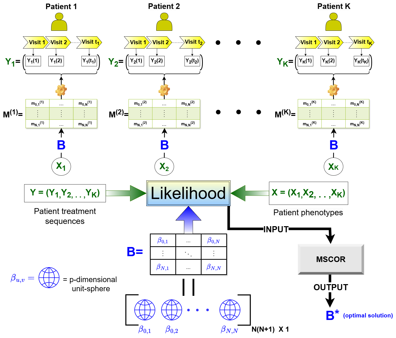
Figure 1: Concept diagram of SMART-MC visually depicting the data structure, likelihood, parameter-space and estimation steps of the analysis.

2.4 Likelihood

To this end, suppose we denote the probability of starting with treatment $T_{1}$ for the $k$-th patient by $s(T_{1}|X_{k})$, and the probability of transition from treatment $T_{t}\rightarrow T_{t+1}$ by $P(T_{t}\rightarrow T_{t+1}|X_{k})$. Suppose, the treatment sequence for the $k$-th patient is $\big{(}T_{1},T_{2},\ldots,T_{t_{k}}\big{)}\equiv\big{(}Y_{k,1},\ldots,Y_{k,t_{k}}\big{)}$. Hence, under Markovian framework, the full likelihood for the entire patient-cohort is given by,

$$P(\bm{Y}_{1},\dots,\bm{Y}_{K}|\bm{B},\bm{X}_{1},\dots,\bm{X}_{K})=\prod_{k=1}^{K}m^{(k)}_{0,Y_{k,1}}m^{(k)}_{Y_{k,1},Y_{k,2}}\cdots m^{(k)}_{Y_{k,t_{k}-1},Y_{k,t_{k}}}.$$ (4)

Note that, due to our proposed constraints of fixing the $l_{2}$ norm of $\bm{\beta}_{u,v}$ to be 1, the likelihood becomes a function of parameters that can be expressed as a collection of spherically constrained unit vectors. Another important consideration is that, the rare transition-based adjustment discussed in Subsection 2.3 renders the likelihood function to be non-concave (verified later on). Thus, maximization of (4) calls for a global optimization algorithm tailored to maximize the multi-modal function of parameters given by a collection of unit spheres, which we specifically develop in the following section, named Multiple Spherically Constrained Optimization Routine (MSCOR). A visual illustration of SMART-MC is shown in Figure 1.

3 MSCOR

To estimate the matrix of coefficient vectors for transitions and initial states, we maximize the likelihood (4). Each coefficient vector, corresponding to ‘non-rare’ cases, lies on the surface of a $p$-dimensional unit sphere (i.e., the space of spherically constrained vectors in $\mathds{R}^{p+1}$). The optimization problem is formulated as:

$$\text{maximize:}\;f:\bm{S}\to\mathds{R},$$

$$\text{subject to:}\;\bm{S}=O^{n_{1}-1}\times\cdots\times O^{n_{B}-1},$$ (5)

where $O^{w-1}=\{(x_{1},\ldots,x_{w})\in\mathds{R}^{w}:\sum_{i=1}^{w}x_{i}^{2}=1\}$. As the likelihood is not concave, a global optimization algorithm is required.

3.1 Background

Optimization has remained a pivotal domain for nearly a century, spanning disciplines such as Mathematics, Engineering, Statistics, and Computer Science. Early approaches focused primarily on convex optimization, renowned for its rapid convergence and ability to estimate large parameter spaces with limited computational resources (Boyd & Vandenberghe, 2004). Methods like the Newton-Raphson algorithm remain widely utilized due to their established efficiency (Nocedal & Wright, 2006). Advances in convex optimization have included techniques such as Interior Point (IP; Potra & Wright, 2000) and Sequential Quadratic Programming (SQP; Wright, 2005). However, these methods face critical limitations in non-convex settings, as they lack mechanisms to escape local optima, necessitating the adoption of global optimization strategies.

The growth of computational power over recent decades has facilitated the development of advanced global optimization methods for addressing non-convex problems. Notable among these are Genetic Algorithms (GA; Fraser, 1957), Simulated Annealing (SA; Kirkpatrick et al., 1983), and Particle Swarm Optimization (PSO; Kennedy & Eberhart, 1995). These heuristic approaches incorporate strategies to bypass local solutions, thereby increasing the likelihood of reaching global optima. Although computationally demanding, leveraging parallel computing can significantly mitigate their computational burden (Cantu-Paz & Goldberg, 2000). We further delineate the fundamental principles and key distinctions between convex and global optimization methodologies from a different perspective, known as ‘exploitation vs exploration’ dilemma.

‘Exploitation vs exploration’ dilemma:

The explore-exploit trade-off addresses the balance between acquiring new information (exploration) and utilizing it for performance improvement (exploitation) (Berger-Tal et al., 2014). This dilemma is critical across disciplines, including numerical optimization (Zhang et al., 2023). Gradient-based methods emphasize full exploitation, optimizing by following the steepest descent direction, while grid search represents full exploration, prioritizing exhaustive evaluation over refinement. In light of recent computational advancements, although fine-grid searches remain infeasible for high-dimensional spaces, they enable us to move beyond a sole exploitation strategy, allowing room for some exploration as well, which is necessary to solve non-convex problems. Parallel computing alleviates some of the associated computational burden, particularly for global optimization methods that integrate exploration and exploitation strategies simultaneously, in a balance fashion (Cantu-Paz & Goldberg, 2000). Global optimization methods balance these extremes, conceptually modeled as

$$\gamma\cdot\textit{exploitation}+(1-\gamma)\cdot\textit{exploration},\quad\gamma\in(0,1),$$

bridging gradient-based methods ($\gamma=1$) and grid search ($\gamma=0$). However, scalability still remains a challenge for many of such existing techniques; for instance, GA face exponential search space growth in high dimensions (Geris, 2012), which can pose challenges in higher dimensional settings.

Recursive Modified Pattern Search:

Pattern Search (PS; Torczon, 1997) have gained noticeable popularity across the domain of Derivative Free Optimization (DFO; Lewis & Torczon, 1999, 2000). The main principle of PS revolves around generating a set of candidate points around the current solution in the update step, and eventually finding the best out of them, moving to next iteration. Despite its extraordinary capability in conducting a substantial exploration over the parameter space along with well-established convergence properties, it lacks mechanisms to escape local optima. To address this limitation, Recursive Modified Pattern Search (RMPS; Das, 2023) incorporates a few necessary adjustments along with pioneering a concept of recursive search technique, further enabling it the ability to escape local solutions. RMPS was shown to outperform GA and SA across benchmarks. Further extensions of RMPS have demonstrated superior performance in constrained parameter spaces such as unit sphere (Das et al., 2022), unit simplex (Das, 2021) and multiple simplexes (Das et al., 2023a). This study further extends RMPS to optimize functions over collections of unit spheres. Additionally, we integrate parallel-threading strategies to enhance computational efficiency, leveraging recent advancements in parallel computing to overcome scalability barriers.

3.2 MSCOR

3.2.1 Fermi’s Principle

The foundation of RMPS, the underlying mechanism of MSCOR, lies in Fermi’s principle (Fermi & Metropolis, 1952), which provides a strategy for exploring the parameter space to optimize an objective function, even when non-differentiable, over an unconstrained domain. According to this principle, at each iteration, the function is evaluated at $2n$ neighboring points, corresponding to coordinate-wise movements in positive or negative directions with a step-size $s>0$. The best-performing point among these is chosen as the updated solution. By varying $s$, candidate points can be generated from either nearby locations (small $s$) or farther neighborhoods (larger $s$), enabling adaptive exploration. Convergence is achieved when no improvement is found as $s\to 0$ (Torczon, 1997; Das, 2023). Figure 2 illustrates the candidate points generated under this principle for a given $s$.

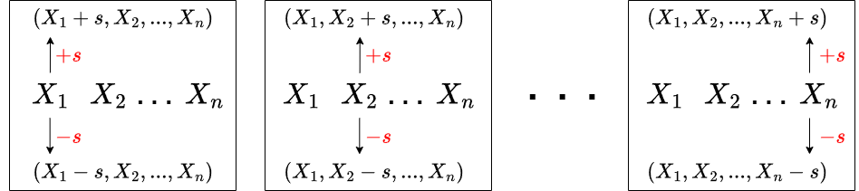
Figure 2: Fermi’s principle : Possible $2n$ movements starting from initial point $(x_{1},\ldots,x_{n})$ inside an iteration with fixed step-size $s$, while optimizing any $n$-dimensional objective function over unconstrained parameter space.

3.2.2 Movements Across Multiple Spherically Constrained Space

In the case of a spherically constrained parameter space, starting from a solution on the unit sphere, moving one coordinate by step-size $s$ renders the updated point infeasible since it no longer resides on the unit sphere. To address this, we propose adjustments to the remaining coordinates to maintain the $l_{2}$-norm of the updated vector as 1. This adjustment, termed the adjustment step-size, is computed to ensure feasibility under such constraints, a step unnecessary in unconstrained optimization. At the $j$-th iteration, let the current solution be $\bm{x}^{(j)}=(x_{1},\ldots,x_{n})$, where $||\bm{x}^{(j)}||_{2}=1$. We generate $2n$ candidate points around $\bm{x}^{(j)}$ using Fermi’s principle. Denote the candidate solution after moving the $i$-th coordinate by $s$ in the positive direction as $\bm{x}^{(i+)}=(x_{1}^{*},\ldots,x_{n}^{*})$, where

$$x_{q}^{*}=\begin{cases}x_{q}+s&\text{if }q=i,\\ x_{q}+t_{i}&\text{if }q\in\{1,\ldots,n\}\setminus\{i\}.\end{cases}$$

To ensure $||\bm{x}^{(i+)}||_{2}=1$, $t_{i}$ is chosen to satisfy the following equation:

$$\sum_{q=1}^{n}(x_{q}^{*})^{2}=\sum_{q=1,q\neq i}^{n}(x_{q}+t_{i})^{2}+(x_{i}+s)^{2}=1.$$ (6)

Solving the resulting quadratic equation for $t_{i}$, we obtain two solutions:

$$t_{i}^{(1)} =\frac{-2\sum_{q=1,q\neq i}^{n}x_{q}+\sqrt{D_{i}(s)}}{2(n-1)},\quad t_{i}^{(2)}=\frac{-2\sum_{q=1,q\neq i}^{n}x_{q}-\sqrt{D_{i}(s)}}{2(n-1)},$$

where, $D_{i}(s)=\left(2\sum_{q=1,q\neq i}^{n}x_{q}\right)^{2}-4(n-1)(2sx_{i}+s^{2})$. To ensure $t_{i}\to 0$ as $s\to 0$, a requirement for establishing convergence properties, the adjustment $t_{i}$ is set to $t_{i}^{(1)}$. However, scenarios where $D_{i}(s)<0$ may arise, making $t_{i}$ nonexistent for certain step-sizes. In practice, these cases are rare; when encountered, $s$ is reduced iteratively until $D_{i}(s)>0$. If this fails, the update is skipped, and subsequent steps are attempted. After generating the candidate points (up to $2n$), function values are evaluated, and the best candidate is chosen. If no candidate improves the objective, the current solution is retained, and $s$ is reduced further (detailed as follows).

Using the updated Fermi’s principle for spherically constrained space, as outlined above, starting from an initial solution, for a given step-size $s$, we can generate up to $2n$ candidate points. Now, consider $B$ unit spheres, each with a length $n_{b}$ for $b=1,\dots,B$. Applying the same principle, we generate $2\sum_{b=1}^{B}n_{b}$ candidate solutions. The current objective function value is then compared with those evaluated at the candidate points, and the best value is selected as the updated solution.

3.2.3 MSCOR Overview

MSCOR operates through several runs, with iterations occurring within each run until a convergence criterion is met, as detailed later on. Each run begins with the solution from the previous run and aims to improve upon it, with the initial solution for the first run provided by the user. Each run starts with a larger step-size (involved in the parameter space exploration, as introduced in Fermi’s principle), which progressively becomes smaller over iterations, eventually becoming very close to zero towards the end of a run. While the larger step-size induces more exploration over the parameter space, later on, decrementing the step-size over iterations emphasizes refining the solution within a close neighborhood, focusing more on exploitation. This strategy resembles the ‘cooling down’ mechanism in SA. At the beginning of a new run, the step-size is again increased to shift the mode of the search strategy back more towards exploration. This strategy precisely helps MSCOR to escape local minima. The algorithm terminates when the solutions from two consecutive runs are sufficiently close, which can be naively interpreted as the message that further exploration within the bounds of MSCOR may not yield a better solution.

Tuning Parameters:

Each run is governed by the following tuning parameters: initial global step-size $s_{\text{initial}}>0$, step decay rate $\rho>1$, step-size threshold $\phi>0$, and sparsity threshold $\lambda\geq 0$. These parameters are set by the user and remain constant across runs. Two additional parameters, $\tau_{1}$ and $\tau_{2}$, control the convergence criteria. Additionally, the maximum number of iterations per run and the maximum number of runs are denoted as MaxIter and MaxRun, respectively.

Global and Local Step-Sizes:

The parameter space consists of multiple unit spheres. Let there be $B$ unit spheres, with the $b$-th block being $(n_{b}-1)$-dimensional and denoted by $\mathbf{O}_{b}=(o_{b,1},\dots,o_{b,n_{b}})\in O^{n_{b}-1}$, for $b=1,\dots,B$. The total number of parameters is $M=\sum_{j=1}^{B}n_{j}$. Within each run, we use a global step-size $\eta$ and $2M$ local step-sizes $\{(s_{b,i}^{+},s_{b,i}^{-})\}_{i=1}^{n_{b}}\}_{b=1}^{B}$, which adapt based on the tuning parameters and improvements in the objective function.

In the first iteration, the global step-size is initialized to $\eta^{(1)}=s_{\text{initial}}$. This global step-size remains constant throughout the iteration (but periodically updated across iterations throughout a run). At the end of each iteration, its value either remains the same or is divided by $\rho$ ($\rho>1$), depending on whether a ‘sufficiently’ better solution was discovered during that iteration (as detailed later). At the start of each iteration, the local step-sizes $s_{b,i}^{+}$ and $s_{b,i}^{-}$ are initialized to the current global step-size $\eta$.

Exploratory movements:

At the beginning of the $h$-th iteration, the current value of the parameters is denoted by $\bm{O}=\bm{O}^{(h)}=(\mathbf{O}_{1}^{(h)},\dots,\mathbf{O}_{B}^{(h)})$, where each $\mathbf{O}_{b}^{(h)}=(o_{b,1}^{(h)},\dots,o_{b,n_{b}}^{(h)})\in O^{n_{b}-1}$ for $b=1,\dots,B$. During the iteration, the objective function is evaluated at up to $2M$ feasible points in the neighborhood of $\mathbf{O}^{(h)}$. These points are derived by exploring candidate points around $\mathbf{O}^{(h)}$, modulated by the local step-sizes $\{(s_{b,i}^{+},s_{b,i}^{-})\}_{i=1}^{n_{b}}\}_{b=1}^{B}$. The feasible exploration directions are classified into $M$ ‘positive’ movements $(b,i,+)$ and $M$ ‘negative’ movements $(b,i,-)$. A coordinate of the unit-sphere is termed ‘significant’ if its value exceeds a sparsity threshold $\lambda$ (detailed later), where $\lambda$ can be set to zero to avoid thresholding. For each $b$, the $b$-th unit-sphere $\mathbf{O}_{b}^{(h)}$ has $m_{b}$ significant locations, excluding the $i$-th location $o_{b,i}^{(h)}$. Except for these $m_{b}+1$ locations (including $i$-th), all others are replaced with zeros. The movement $(b,i,+)$ involves updating $o_{b,i}^{(h)}$ by adding $s_{b,i}^{+}$ to it, and adjusting the ‘significant’ locations with an ‘adjustment step-size’, ensuring the updated point maintains a zero $l_{2}$ norm. If the updated value exceeds the unit-sphere boundary, or the adjustment step-size is invalid, the local step-size is reduced by a factor of $\rho$ (ensuring $s_{b,i}^{+}>\phi$) and the update is attempted again until the point remains within the unit-sphere. In rare cases where no feasible candidate is found, $\mathbf{O}_{b}^{(h)}(i,+)$, proposal candidate point corresponding to movement $(b,i,+)$, remains unchanged, same as $\bm{O}_{b}^{(h)}$. The $(b,i,-)$ movement follows a similar process by subtracting $s_{b,i}^{-}$ followed by ‘adjustment’ of the significant locations accordingly. Finally, the best candidate point is chosen from $2M+1$ candidate points, including $\bm{O}^{(h)}$.

Algorithm 1 MSCOR

1:Input: Initial guess; ($B$ blocks of $(n_{b}-1)$-dimensional unit spheres; $b=1,\ldots,B$)

2:Output: $\widehat{\bm{U}}$; MSCOR optimized final solution ($B$ blocks of $(n_{b}-1)$-dimensional unit spheres; $b=1,\ldots,B$)

3:Initialization: $R\leftarrow 1$ ($R$ = run index)

4:top:

5:if $R=1$ then

6:  $\bm{U}^{(0)}\leftarrow\text{Initial guess},\;j\leftarrow 1$ ($\bm{U}^{(j)}$ denotes the value of $\bm{U}$ at the end of $j$-th iteration)

7:else

8:  $\bm{U}^{(0)}\leftarrow\widehat{\bm{U}}^{(R-1)},\;j\leftarrow 1$ ($\widehat{\bm{U}}^{(r)}$ denotes the value of $\bm{U}$ at the end of $r$-th run)

9:$s^{(0)}\leftarrow s_{initial}$ (we take $s_{initial}=1$; $s^{(j)}$ denotes the value of global step-size at the end of $j$-th iteration)

10:while ($j\leq max\_iter$ and $s^{(j)}>\phi$) do

11:  $F_{1}\leftarrow f(\bm{U}^{(j-1)})$, $s\leftarrow s^{(j-1)}$ (note that, $\bm{U}^{(j-1)}=(\bm{u}_{1}^{(j-1)},\ldots,\bm{u}_{B}^{(j-1)})$)

12:  for $b=1:B$ do

13:   for $h=1:2n_{b}$ do

14:     $i\leftarrow[\frac{(h+1)}{2}]$ ($[\cdot]$ denotes largest smaller integer function)

15:     $\bm{u}_{b,h}\leftarrow\bm{u}_{b}^{(j-1)}$(note that, $\bm{u}_{b,h}=\big{(}\bm{u}_{b,h}(1),\ldots,\bm{u}_{b,h}(n_{b})\big{)}$)

16:     $s_{h}\leftarrow(-1)^{h}s$

17:     $\Lambda\leftarrow\text{which}(|\bm{u}_{b,h}(k)|<\lambda),k\in\{1,\ldots,n_{b}\}\setminus\{i\}$ (i.e., indexes, except $i$, whose absolute values are $<\lambda$)

18:     $\Gamma\leftarrow\text{which}(|\bm{u}_{b,h}(k)|\geq\lambda),k\in\{1,\ldots,n_{b}\}\setminus\{i\}$ (i.e., indexes, except $i$, whose absolute values are $\geq\lambda$)

19:     $D\leftarrow\big{(}2*sum(\bm{u}_{b,h}(\Gamma)))^{2}-4*length(\Gamma)*(2s_{h}\bm{u}_{b,h}(i)+s_{h}^{2}-sumsquare(\bm{u}_{b,h}(\Lambda)))$.

20:     while ($D<0$ and $|s_{h}|>\phi$) do

21:      $s_{h}\leftarrow\frac{s_{h}}{\rho}$

22:      $D\leftarrow\big{(}2*sum(\bm{u}_{b,h}(\Gamma)))^{2}-4*length(\Gamma)*(2s_{h}\bm{u}_{b,h}(i)+s_{h}^{2}-sumsquare(\bm{u}_{b,h}(\Lambda)))$.      

23:     if ($D\geq 0$) then

24:      $t\leftarrow\frac{-2*sum(\bm{u}_{b,h}(\Gamma))+\sqrt{D}}{2*length(\Gamma)}$

25:      $\bm{u}_{b,h}(i)\leftarrow\bm{u}_{b,h}(i)+s_{h}$

26:      $\bm{u}_{b,h}(\Gamma)\leftarrow\bm{u}_{b,h}(\Gamma)+t$

27:      $\bm{u}_{b,h}(\Lambda)\leftarrow 0$

28:      $f_{b,h}\leftarrow f(\bm{u}_{1}^{(j-1)},\ldots,\bm{u}_{b-1}^{(j-1)},\bm{u}_{b,h},\bm{u}_{b+1}^{(j-1)},\ldots,\bm{u}_{B}^{(j-1)})$

29:     else

30:      $f_{b,h}\leftarrow F_{1}$ ($\bm{u}_{b,h}$ remains unchanged, no update is made)           

31:  $(b_{best},h_{best})\leftarrow\operatorname*{arg\,min}_{b,h}f_{b,h}$ over $b=1,\ldots,B$, $h=1,\ldots,2n_{b}$

32:  $\bm{u}_{temp}\leftarrow\bm{u}_{b_{best},h_{best}}$

33:  $F_{2}\leftarrow f_{b_{best},h_{best}}$

34:  $\bm{U}^{(j)}\leftarrow\bm{U}^{(j-1)}$

35:  if ($F_{2}<F_{1}$) then $\bm{u}^{(j)}_{b_{best}}\leftarrow\bm{u}_{temp}$ (hence $\bm{U}^{(j)}$ becomes $\big{(}\bm{u}_{1}^{(j-1)},\ldots,\bm{u}_{b_{best}-1}^{(j-1)},\bm{u}_{temp},\bm{u}_{b_{best}+1}^{(j-1)},\ldots,\bm{u}_{B}^{(j-1)}\big{)}$ )   

36:  if ($j>1$) then

37:   if ($|F_{1}-min(F_{1},F_{2})|<\tau_{1}$ and $s>\phi$) then $s\leftarrow\frac{s}{\rho}$      

38:  $s^{(j)}\leftarrow s$, $j\leftarrow j+1$

39:$\widehat{\bm{U}}^{(R)}\leftarrow\bm{U}^{(j)}$

40:if $||\widehat{\bm{U}}^{(R)}-\widehat{\bm{U}}^{(R-1)}||<\tau_{2}$  then

41:  return $\widehat{\bm{U}}=\widehat{\bm{U}}^{(R)}$ (returning MSCOR optimized final solution $\widehat{\bm{U}}$)

42:  break (exiting MSCOR)

43:else

44:  $R\leftarrow R+1$

45:  go to top

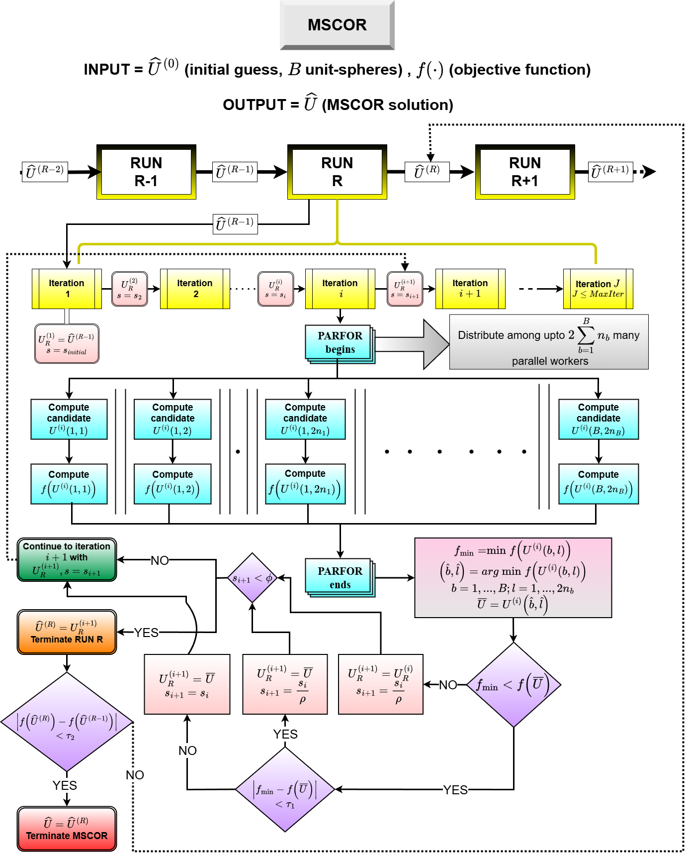
Figure 3: MSCOR flowchart.

Sparsity control:

We introduce a sparsity control step to promote sparse solutions. For each modified unit-sphere $\{\mathbf{O}_{j}^{(h)}(i,+)\}_{i=1}^{n_{b}}$ and $\{\mathbf{O}_{j}^{(h)}(i,-)\}_{i=1}^{n_{b}}$ for $b=1,\dots,B$, we zero out the values of coordinates deemed ‘insignificant’ (those less than $\lambda$). To preserve the $l_{2}$ constraint to be 1, the ‘significant’ coordinates are updated by corresponding calculated ‘adjustment step-size’.

Remark 1.

The parameter $\lambda$ should be set relatively large if prior knowledge suggests that the final solution is sparse; otherwise, it can be chosen to be smaller or set to zero.

Loop termination criteria:

At each iteration, the value of $\eta$ either remains unchanged or is divided by $\rho$. If $|f(\mathbf{O}^{(h+1)})-f(\mathbf{O}^{(h)})|<\tau_{1}$ at the end of iteration $(h+1)$, $\eta$ is updated as $\eta=\eta/\rho$ (ensuring $\eta>\phi$); otherwise, it remains unchanged. Once $\eta$ becomes less than $\rho$, the run terminates, forwarding the last obtained solution (denote it by $\mathbf{\hat{O}}^{(L)}$ for the $L$-th run) to the next run to serve as the starting point for that run. MSCOR terminates when the solutions obtained by two consecutive runs, say $R-1$ and $R$, satisfy $|f(\mathbf{\hat{O}}^{(R)})-f(\mathbf{\hat{O}}^{(R-1)})|<\tau_{2}$. A flowchart of the MSCOR algorithm is shown in Figure 3, and pseudo-code is provided in Algorithm 1.

Parallelized MSCOR:

Close inspection of the MSCOR exploration strategy reveals that for any given step-size, the exploration and evaluation of the objective functions at the corresponding up to $2M$ candidate points are independent of each other, allowing these updates to be performed simultaneously within each iteration across $2M$ parallel threads, further alleviating the computational burden (as illustrated in Figure 3).

Convex optimization and non-conxexity detection using MSCOR:

If the objective function is known to be convex a priori, a single run suffices, as the stopping criterion ensures local optimality (details provided in the following subsection). In the absence of prior information about convexity, MSCOR automatically terminates after the second run, since each run converges to an optimal solution. For convex functions, this solution is unique, resulting in identical outcomes in the first two consecutive runs, thereby satisfying the stopping criterion. Consequently, MSCOR efficiently terminates early for convex functions, significantly reducing computational time. Extending this logic, if MSCOR converges after run $R>2$, it indicates at least one successful escape from a local solution, confirming the presence of multiple optima and hence the non-convexity of the objective function. When optimizing the SMART-MC likelihood with MSCOR, the observed number of runs required for convergence ranges from 5 to 10, corroborating the non-convexity of the likelihood.

3.3 Theoretical property

Here we establish the convergence property of MSCOR. Specifically, we show that the stopping criteria across all runs ensure each solution is optimal under certain regularity conditions. The proof of this theorem is detailed in Section A of the supplementary material. While this result does not strongly demonstrate MSCOR’s global optimization capability, we validate it empirically through an extensive benchmark study in the following subsection.

Definition 1.

The ‘shadow’ of a point $\bm{W}$ (denoted by $\bm{W}^{C}$) belonging to the closure of $\bm{S}$ (i.e., $\bar{\bm{S}}$) is the point of intersection of the straight line connecting the origin to $\bm{W}$ with $\bm{S}$, where $\bm{S}=O^{n_{1}-1}\times\dots\times O^{n_{B}-1}$.

Theorem 1.

Suppose $f:\bm{S}\mapsto\mathds{R}$ is convex, continuous and differentiable with extended definition on $\bar{\bm{S}}$, such that, $f(\bm{W})=f(\bm{W}^{C})$ when $\bm{W}\in interior(\bm{S})$. Consider a sequence $\delta_{j,k}=\frac{s_{j}}{\rho^{k}}$ for $k\in\mathds{N}$ and $s_{j}>0,\rho>1$. Suppose $\mathbf{U}\in\bm{S}$ given by

$$\mathbf{U}=(\mathbf{u}_{1},\ldots,\mathbf{u}_{B})\text{ where }\mathbf{u}_{b}=(u_{j,1},\ldots,u_{j,n_{b}})\in O^{n_{j}-1},\;j=1,\ldots,B.$$

Define, $\mathbf{u}_{j,k}^{(i+)}=(u_{j,1}+t_{i}(\delta_{j,k}),\ldots,u_{j,i-1}+t_{i}(\delta_{j,k}),u_{j,i}+\delta_{j,k},u_{j,i+1}+t_{i}(\delta_{j,k}),\ldots,u_{j,n_{j}}+t_{i}(\delta_{j,k}))$, $\mathbf{u}_{j,k}^{(i-)}=(u_{j,1}+t_{i}(-\delta_{j,k}),\ldots,u_{j,i-1}+t_{i}(-\delta_{j,k}),u_{j,i}-\delta_{j,k},u_{j,i+1}+t_{i}(-\delta_{j,k}),\ldots,u_{j,n_{j}}+t_{i}(-\delta_{j,k}))$ for $j=1,\ldots,B$, $i=1,\cdots,n_{j}$, where $t_{i}(s)$ denotes the adjustment step-size corresponding to step-size $s$. Define $b_{j,i}=-\frac{u_{j,i}}{\big{|}\sum_{k=1,k\neq i}^{n_{j}}u_{j,k}\big{|}}$. If the following conditions hold true

1. for all sufficiently large $k\in\mathrm{N}$, $f(\mathbf{U})\leq f(\mathbf{u}_{1},\ldots,\mathbf{u}_{j-1},\mathbf{u}_{j,k}^{(i+)},\mathbf{u}_{j+1},\ldots,\mathbf{u}_{B})$ and $f(\mathbf{U})\leq f(\mathbf{u}_{1},\ldots,\mathbf{u}_{j-1},\mathbf{u}_{j,k}^{(i-)},\mathbf{u}_{j+1},\ldots,\mathbf{u}_{B})$

2. $1-b_{j,i}\neq 0$

3. $\big{[}(n_{j}-2)+\sum_{i=1}^{n_{j}-1}\frac{1}{1-b_{j,i}}\big{]}\neq 0$

for $j=1,\ldots,B$, $i=1,\ldots,n_{j}-1$, then a global minimum of $f$ over $\mathbf{S}$ occurs at $\mathbf{U}$.

3.4 Benchmark Study of Global Optimization

In order to evaluate the comparative performance of MSCOR, we consider the minimization problem of four benchmark functions, namely the Rastrigin function, Ackley’s function, Sphere function, and Griewank function (Jamil & Yang, 2013), with their parameter spaces modified to be collections of unit spheres (see Section B of the supplementary material). MSCOR is implemented in MATLAB and executed on a desktop running the Windows 10 Enterprise operating system with 32 GB RAM and the following processor specifications: 12th Gen Intel(R) Core(TM) i7-12700, 2100 MHz, 12 Cores, and 20 Logical Processors. MSCOR is compared with GA, SA, SQP, IP, and Active-set (AS) optimization methods; the first two being global optimizers, and the rest being convex optimizers. We use MATLAB’s built-in toolbox functions ga (for GA), simulannealbnd (for SA), and fmincon (for IP, SQP, and AS) to implement the respective algorithms. We consider the scenarios $(B,n_{b})=(5,5),(10,20),(100,5)$, where the dimension of the last scenario closely resembles to that of the case study discussed later. For each scenario, the experiment is repeated 100 times, each time starting from a different randomly generated initial point. The results are summarized in Table 1. We observe that MSCOR consistently outperforms all other methods by a substantial margin, yielding better solutions than its competitors within a reasonable time frame. Additionally, MSCOR allows users to set an upper bound on the computation time, in which case it returns the best solution found within the allotted time. Such a scenario is encountered while optimizing Ackley’s and Griewank functions, where MSCOR terminated at the end of 1 hour (the set upper bound). Although MSCOR had the potential to further improve the solutions, the results obtained within 1 hour still outperformed most of the other competitors. Lastly, although parallel MSCOR could have substantially improved computation time, we refrain from using it to ensure a fair comparison, as not all competitor algorithms are parallelizable.

Functions	Algorithms	$B=5,n_{b}=5$			$B=10,n_{b}=20$			$B=100,n_{b}=5$
		min. value	se of solution	mean time (se)	min. value	se of solution	mean time (se)	min. value	se of solution	mean time (se)
Ackley’s (modified)	MSCOR	2.22e - 14	0.029	1.64 (0.008)	3.61e - 13	0.000	312.58 (0.385)	1.65e - 09	0.288	3600.04∗(0.006)
	GA	1.51e + 01	0.169	16.34 (0.769)	2.59e + 01	0.080	78.81 (0.315)	3.88e + 02	2.214	357.20 (3.682)
	SA	4.70e + 00	0.081	1.84 (0.092)	2.16e + 01	0.039	53.48 (2.490)	2.70e + 02	1.175	371.77 (23.565)
	IP	7.51e - 12	0.347	0.06 (0.003)	3.67e - 03	0.023	0.09 (0.002)	2.17e + 02	6.179	0.42 (0.026)
	SQP	9.50e - 04	0.414	0.03 (0.001)	1.28e - 02	0.000	0.41 (0.001)	8.33e + 01	9.219	5.15 (0.028)
	AS	2.35e + 00	0.328	0.03 (0.001)	1.53e + 00	0.401	0.47 (0.003)	1.56e + 02	4.564	5.60 (0.010)
Griewank (modified)	MSCOR	<1e - 16	0.000	1.54 (0.007)	1.78e - 15	0.000	204.51 (0.444)	1.46e - 09	0.000	3600.07∗(0.010)
	GA	8.04e - 01	0.040	19.59 (0.962)	1.12e + 00	0.021	88.70 (0.287)	3.60e + 01	0.400	461.57 (4.188)
	SA	1.06e - 01	0.008	2.03 (0.101)	7.99e - 01	0.004	54.12 (2.392)	2.72e + 01	0.166	372.25 (11.450)
	IP	2.47e - 13	0.000	0.02 (0.002)	6.53e - 04	0.000	0.10 (0.002)	2.03e + 00	0.175	0.50 (0.025)
	SQP	1.98e - 13	0.000	0.01 (0.000)	5.96e - 12	0.000	0.24 (0.001)	3.80e - 12	0.000	1.69 (0.015)
	AS	3.50e - 08	0.022	0.03 (0.002)	2.77e - 07	0.005	0.43 (0.015)	4.54e - 07	0.464	5.79 (0.722)
Neg. sum of squares (modified)	MSCOR	<1e - 16	0.000	0.45 (0.005)	<1e - 16	0.000	43.81 (0.413)	1.51e - 14	0.000	1602.09 (15.515)
	GA	5.17e + 00	0.198	16.47 (0.805)	8.27e + 01	0.648	74.74 (0.258)	1.89e + 02	2.398	325.61 (2.558)
	SA	2.19e + 00	0.044	1.85 (0.087)	7.10e + 01	0.126	50.59 (2.549)	1.65e + 02	0.435	358.06 (16.27)
	IP	7.99e - 15	0.000	0.02 (0.000)	1.26e + 00	0.100	0.09 (0.002)	3.83e + 00	1.520	0.40 (0.023)
	SQP	1.07e - 14	0.000	0.02 (0.000)	4.26e - 07	0.000	0.41 (0.002)	9.09e - 12	0.000	3.78 (0.102)
	AS	1.92e - 09	0.093	0.02 (0.001)	1.60e + 01	0.714	0.45 (0.003)	2.42e + 01	3.595	5.53 (0.093)
Rastrigin (modified)	MSCOR	<1e - 16	0.762	2.08 (0.417)	8.53e - 13	0.000	135.99 (0.255)	1.02e + 02	5.544	3600.04∗(0.011)
	GA	9.90e + 01	5.792	18.21 (0.835)	1.59e + 03	9.215	79.37 (0.262)	4.98e + 03	73.999	412.85 (51.696)
	SA	8.64e + 00	0.302	1.76 (0.082)	3.47e + 01	2.006	93.74 (3.322)	4.72e + 02	10.532	935.30 (60.66)
	IP	6.72e + 00	0.725	0.04 (0.001)	1.68e - 04	5.922	0.10 (0.001)	5.14e + 02	111.633	0.41 (0.010)
	SQP	8.18e + 00	0.637	0.03 (0.000)	7.04e + 00	3.435	0.42 (0.002)	4.71e + 02	10.107	5.32 (0.075)
	AS	1.20e + 00	0.969	0.03 (0.000)	2.19e + 02	21.095	0.46 (0.001)	8.49e + 02	104.721	5.78 (0.058)

Table 1: A comparative study of MSCOR, GA, SA, IP, SQP and AS methods for optimizing modified Ackley, Griewank, negative sum of squares, and Rastrigin functions is presented for cases with parameter settings $(B,n_{b})=(5,5),(10,20),(100,5)$. Each experiment is repeated 100 times. S.e. denotes the standard error. Time is measured in seconds. For the scenarios where MSCOR’s average computation time exceeds upper bound 3600 seconds, are labeled with ^∗.

4 Simulation Study

To evaluate the performance of SMART-MC, backed by MSCOR for optimizing the likelihood, we generate synthetic data with parameter dimensions similar to the real data used in the case study discussed in Section 5. We consider $N=10$ states, $K=1000$ patients, and a sample state sequence length of $t_{k}=20$ across all patients. We generate $p=5$ patient-level covariates for each subject, sampled from $N(0,1)$. The true transition matrix, including the initial state vector, is taken to be $67\%$ sparse, ensuring that each row contains at least two non-zero elements, including transitions within the same state. This is inspired by the fact that it is typical for an MS patient to mostly remain on the same treatment, occasionally moving to a different one. Non-zero transition locations have coefficients drawn from $N(0,10^{2})$, which are later scaled to have an $l_{2}$ norm of 1. MSCOR is then fitted to estimate the coefficient vectors.

We estimate the coefficient vectors corresponding to the top 10 most frequent transitions, as well as the most frequent initial state. The comparison table is provided in Section C of the supplementary material. We observe that MSCOR performs well in estimating these coefficients, with values close to the true ones. To empirically assess whether the estimated coefficients converge to their true values, We calculate the mean absolute deviation (MAD) for the coefficients corresponding to the top 10 transitions, excluding less frequent transitions due to their potential unreliability arising from lower empirical transition counts. MAD is computed for $K=1000,2000,3000$ and $t_{k}=20,40,60$ for all patients, keeping $N=10$. The corresponding table is provided in Section C of the supplementary material. We note that as the sample size and/or observed state sequence length increases, MAD decreases, reducing from $0.0296$ to $0.0096$ as we move from $(K,t_{k})=(1000,20)$ to $(K,t_{k})=(3000,60)$.

To assess the computational gain of parallelized MSCOR, we compare computation times across scenarios $(K,t_{k})=(1000,10),(1000,20),(2000,20)$ and $N=6,9,12$, keeping $t_{k}=20$. Computations are performed in MATLAB using 12 CPU cores. The results are presented in Table 2. Parallelized MSCOR achieves a 3–7 fold speedup over regular MSCOR, with greater gains observed as the parameter dimensions increase. This is expected since computational gains with parallel computing tend to increase as the objective function evaluation becomes more expensive (MathWorks, 2024).

Num. covariates	Num. treatments	Number of parameters	$K=1000,t_{k}=10$			$K=1000,t_{k}=20$			$K=2000,t_{k}=20$
			MSCOR time (sec)	par-MSCOR time (sec)	Speed improvement	MSCOR time (sec)	par-MSCOR time (sec)	Speed improvement	MSCOR time (sec)	par-MSCOR time (sec)	Speed improvement
$p=3$	$N=6$	168	38	10	3.8x	43	11	3.9x	95	31	3.1x
	$N=9$	360	204	32	6.4x	252	40	6.3x	587	96	6.1x
	$N=12$	624	1198	178	6.7x	1502	211	7.1x	3253	501	6.5x
$p=5$	$N=6$	252	53	10	5.3x	57	11	5.2x	136	22	6.2x
	$N=9$	540	328	52	6.3x	443	71	6.2x	1014	163	6.2x
	$N=12$	936	2158	344	6.3x	2825	455	6.2x	7077	1082	6.5x
$p=8$	$N=6$	378	120	24	5.0x	159	29	5.5x	315	54	5.8x
	$N=9$	810	744	119	6.3x	923	143	6.5x	2057	337	6.1x
	$N=12$	1404	4127	634	6.5x	4881	765	6.4x	12697	1931	6.6x

Table 2: Time comparisons between MSCOR and parallel-MSCOR for different numbers of covariates ($p$) and distinct treatment options ($N$) are evaluated for three data sizes. Specifically, $(K,t_{k})=(1000,10),(1000,20),(2000,20)$, where $K$ denotes the number of patients, and $t_{k}$ denotes the length of the generated treatment sequence for each patient.

5 Multiple Sclerosis temporal DMT sequence analysis

We utilize MS DMT sequence data from an EHR cohort at the Massachusetts General and Brigham hospital system (Boston, US), which includes the Comprehensive Longitudinal Investigation of Multiple Sclerosis at Brigham and Women’s Hospital (CLIMB) cohort (Liang et al., 2022; Xia et al., 2013). This dataset contains patient-level information on DMTs alongside clinical and demographic variables. Twelve DMTs are available for MS patients: alemtuzumab (Ale), cyclophosphamide(Cyc), daclizumab, dimethyl fumarate(DF), fingolimod(Fin), glatiramer acetate(GA), interferon-beta(IB), mitoxantrone(Mit), natalizumab(Nat), ocrelizumab, rituximab, and teriflunomide(Ter). Since daclizumab has been withdrawn and few patients received it, we exclude it from analysis by omitting the corresponding encounters. Rituximab and ocrelizumab are grouped under the same mechanistic category (B-cell depletion; referred as BcD). Consequently, the analysis considers ten DMT categories, forming the state-space of our Markov model. To ensure data reliability, we include only patients who initiated MS DMTs on or after January 1, 2006, when electronic prescriptions were implemented in the Mass General Brigham system. To prevent over-counting consecutive visits listing the same DMT within short intervals, we aggregate observations into three-month clusters from the DMT start date. Within each three-month period, identical consecutive DMTs are treated as a single observation. For instance, if all encounters within a three-month period are $A$, such as $A\to A\to A$, the observation is recorded as $A$. If a sequence within the period includes distinct consecutive DMTs, e.g., $A\to A\to B\to B\to A\to C\to C$, the reduced sequence is $A\to B\to A\to C$, representing the period’s unique transitions.

In the EHR cohort, we consider only patients with available clinical and demographic data, alongside MS DMT sequence data, who initiated MS DMT on or after 2006. Applying these filters results in a cohort of 822 patients for clustering analysis. For the SMART-MC analysis, we include covariates commonly used in MS research: age at diagnosis, disease duration, gender, and race (categorized as White, Black, or other). Here, disease duration is defined as the time elapsed from the year of first neurological symptom to the DMT start year. Age and disease duration (in months) are re-centered and re-scaled, detailed in Section D of the supplementary material.

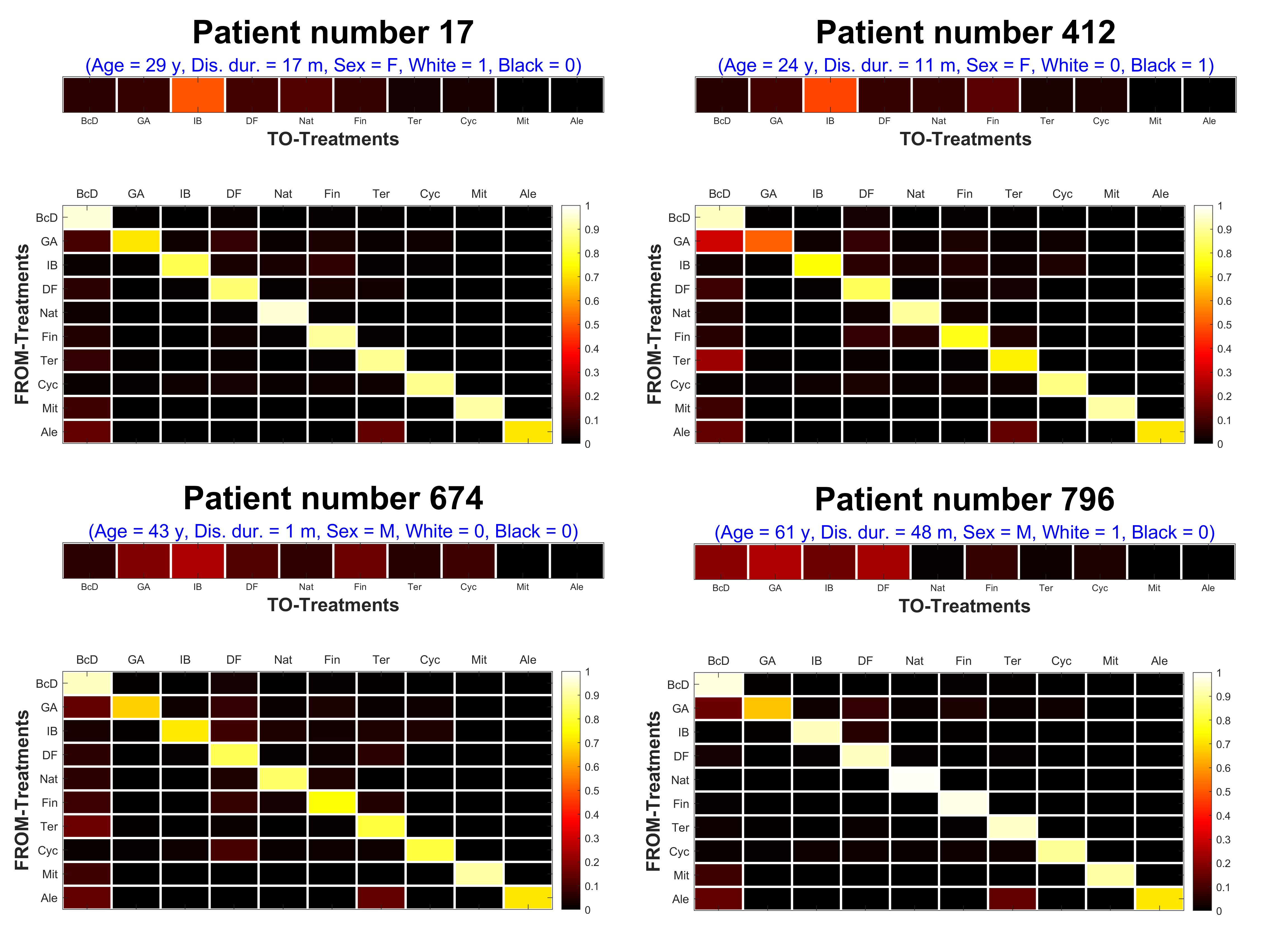
Figure 4: SMART-MC estimated patient-specific initial state probabilities and transition probabilities (upper and lower portions of each sub-figure, respectively) for four patients (serial numbers 17, 412, 674, 796). For each patient, the values of covariates (age at diagnosis, disease duration, sex, race) are provided in the subheadings.

Transitions	Transition counts	Intercept	Age at diagnosis	Disease duration	Sex (Female)	Race: White	Race: Black
Nat $\mapsto$ Nat	2188 (25.31%)	0.70 (0.004)	0.26 (0.004)	0.22 (0.004)	0.14 (0.004)	0.47 (0.004)	0.21 (0.006)
IB $\mapsto$ IB	1682 (19.45%)	0.79 (0.005)	0.32 (0.004)	0.14 (0.004)	0.09 (0.005)	0.48 (0.005)	0.17 (0.006)
Fin $\mapsto$ Fin	1151 (13.31%)	0.70 (0.005)	0.48 (0.005)	0.24 (0.005)	0.09 (0.007)	0.45 (0.005)	0.05 (0.009)
BcD $\mapsto$ BcD	1031 (11.92%)	0.80 (0.010)	0.21 (0.008)	0.37 (0.008)	0.35 (0.009)	0.22 (0.008)	0.08 (0.010)
DF $\mapsto$ DF	934 (10.80%)	0.63 (0.006)	0.33 (0.005)	0.43 (0.006)	0.16 (0.006)	0.32 (0.007)	0.42 (0.009)
Cyc $\mapsto$ Cyc	445 (5.15%)	0.79 (0.009)	0.17 (0.008)	0.11 (0.008)	0.20 (0.009)	0.39 (0.008)	0.39 (0.010)
Ter $\mapsto$ Ter	272 (3.15%)	0.20 (0.009)	0.23 (0.008)	-0.56 (0.010)	0.68 (0.011)	0.36 (0.010)	-0.06 (0.012)
GA $\mapsto$ GA	100 (1.16%)	-0.11 (0.010)	0.59 (0.009)	-0.71 (0.011)	0.24 (0.014)	0.25 (0.011)	-0.15 (0.013)
IB $\mapsto$ Fin	96 (1.11%)	-0.67 (0.009)	-0.27 (0.005)	0.05 (0.006)	0.27 (0.008)	0.43 (0.009)	-0.47 (0.011)
IB $\mapsto$ DF	76 (0.88%)	-0.71 (0.005)	0.14 (0.004)	0.19 (0.005)	-0.59 (0.006)	-0.30 (0.006)	0.01 (0.009)
Fin $\mapsto$ BcD	62 (0.72%)	-0.81 (0.009)	0.29 (0.006)	-0.07 (0.007)	0.06 (0.010)	-0.05 (0.010)	-0.50 (0.015)
IB $\mapsto$ Nat	59 (0.68%)	-0.02 (0.011)	-0.33 (0.005)	-0.56 (0.007)	0.17 (0.010)	0.23 (0.011)	-0.71 (0.013)
DF $\mapsto$ BcD	57 (0.66%)	-0.51 (0.011)	-0.11 (0.006)	0.43 (0.008)	-0.48 (0.011)	0.20 (0.010)	0.51 (0.015)
Nat $\mapsto$ BcD	41 (0.47%)	-0.70 (0.005)	-0.12 (0.005)	-0.08 (0.006)	-0.14 (0.006)	-0.63 (0.005)	-0.28 (0.008)
Nat $\mapsto$ Fin	31 (0.36%)	-0.52 (0.005)	-0.27 (0.005)	-0.33 (0.006)	-0.21 (0.007)	-0.52 (0.005)	-0.49 (0.008)

Table 3: SMART-MC estimated coefficient values corresponding to the top 15 most frequent treatment transitions across Multiple Sclerosis patients are reported, along with the corresponding transition counts (transition proportions). Bootstrap standard errors are listed in parentheses next to the estimated coefficient values. Estimated negative coefficient values are highlighted in red.

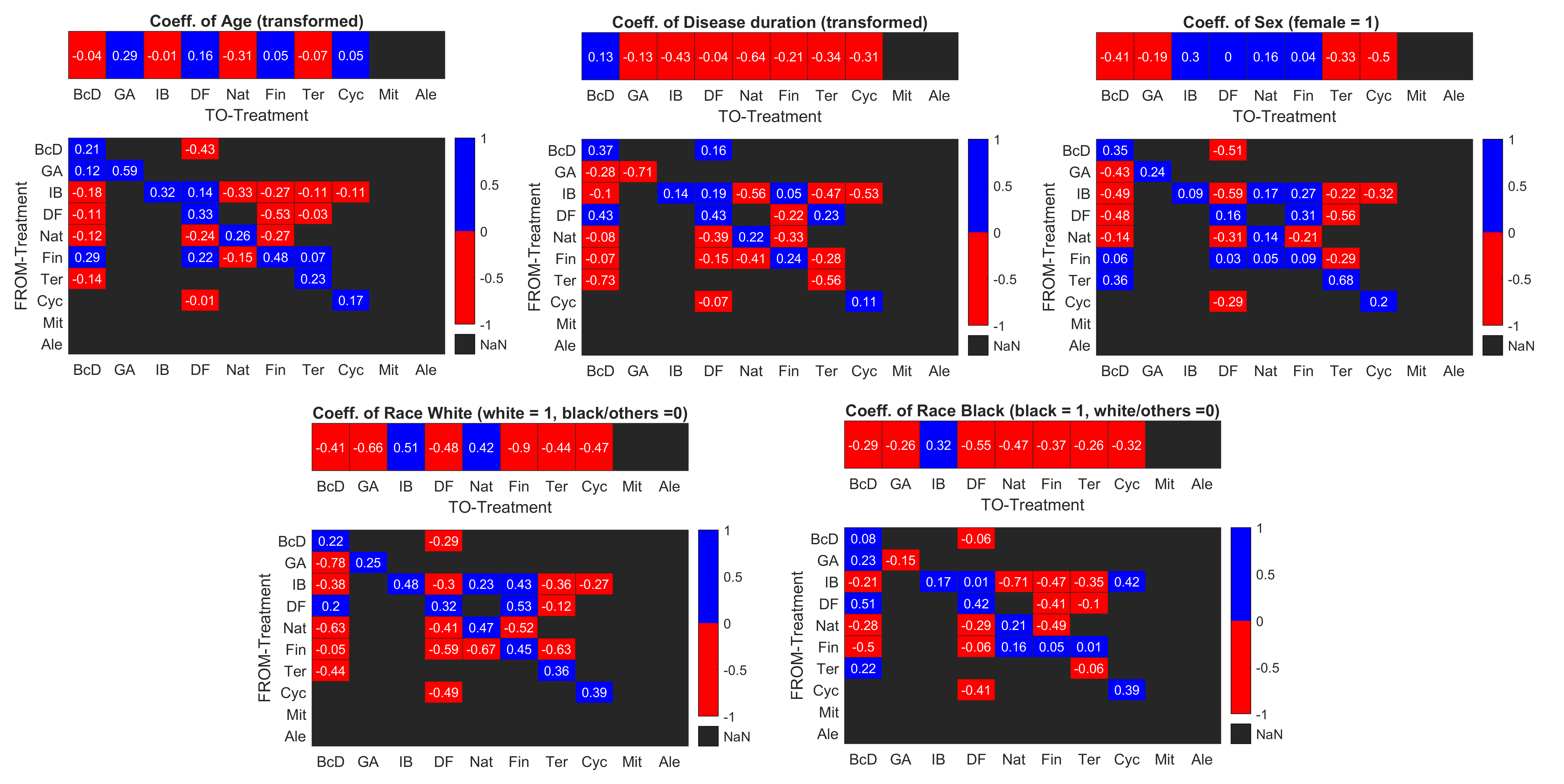
Figure 5: SMART-MC estimated the initial state and transition-specific coefficients (displayed in the upper and lower portions of each sub-figure, respectively) for patient covariates (age at diagnosis, disease duration, sex, race: White, race: Black) are depicted. Positive and negative coefficient values are depicted in blue and red, respectively. Covariate coefficients corresponding to transitions that are not estimated as functions of covariates (but as constants, due to lower number of empirical transition counts) are colored Black.

SMART-MC is employed to examine how patient phenotypes influence transition probabilities across DMTs in MS patients. Figure 4 presents DMT transition matrices for four sample patients, illustrating how SMART-MC estimates patient-specific transition matrices that vary with patient-specific phenotypes. We identify 36 out of the 110 initial states and transitions as non-rare. Consequently, the initial state and transition probabilities estimated by SMART-MC for DMT can only vary at those locations across patients . Table 3 shows the estimated coefficients (with bootstrap standard errors in parentheses) contributing to the corresponding transition probabilities for the 15 most frequent transitions, with negative coefficients highlighted in red. Coefficients for non-rare transitions are further visualized in Figure 5. It is observed that higher age at diagnosis is positively associated with remaining on the same treatment, while negatively associated with transitions to other treatments, consistent with findings in Balusha & Morrow (2024). A similar relationship is noted with disease duration, except for a negative association with staying on Ter and GA long-term. Compared to males, females tend to remain on Ter and BcD longer, while being less prone to transitions such as IB to DF and DF to BcD. Females, in general, show an overall tendency to be more likely to stay on the same treatment compared to males.

Key differences between Black and White populations are further identified in terms of transitions across treatments. For instance, transitions from IB to Fin and Nat are more likely for Whites than Blacks, with the White population generally showing a greater tendency to stay on the same treatment. Additionally, transitions from Nat to BcD and Fin are less likely for both White and Black populations than other races. To further explore the impact of patient phenotypes on treatment transition dynamics, we consider the seven most frequent transitions to different DMTs and compare their odds ratios relative to remaining on the same treatment. Based on the trained model, these odds ratios are estimated across two representative ages (30 and 60), sex (M/F), and race (White/Black/others), and are calculated at all three quartiles of disease duration, as shown in Figure 6. The results further underscore that younger patients exhibit a greater tendency to transition to a different treatment, a pattern more pronounced in non-Black and non-White populations.

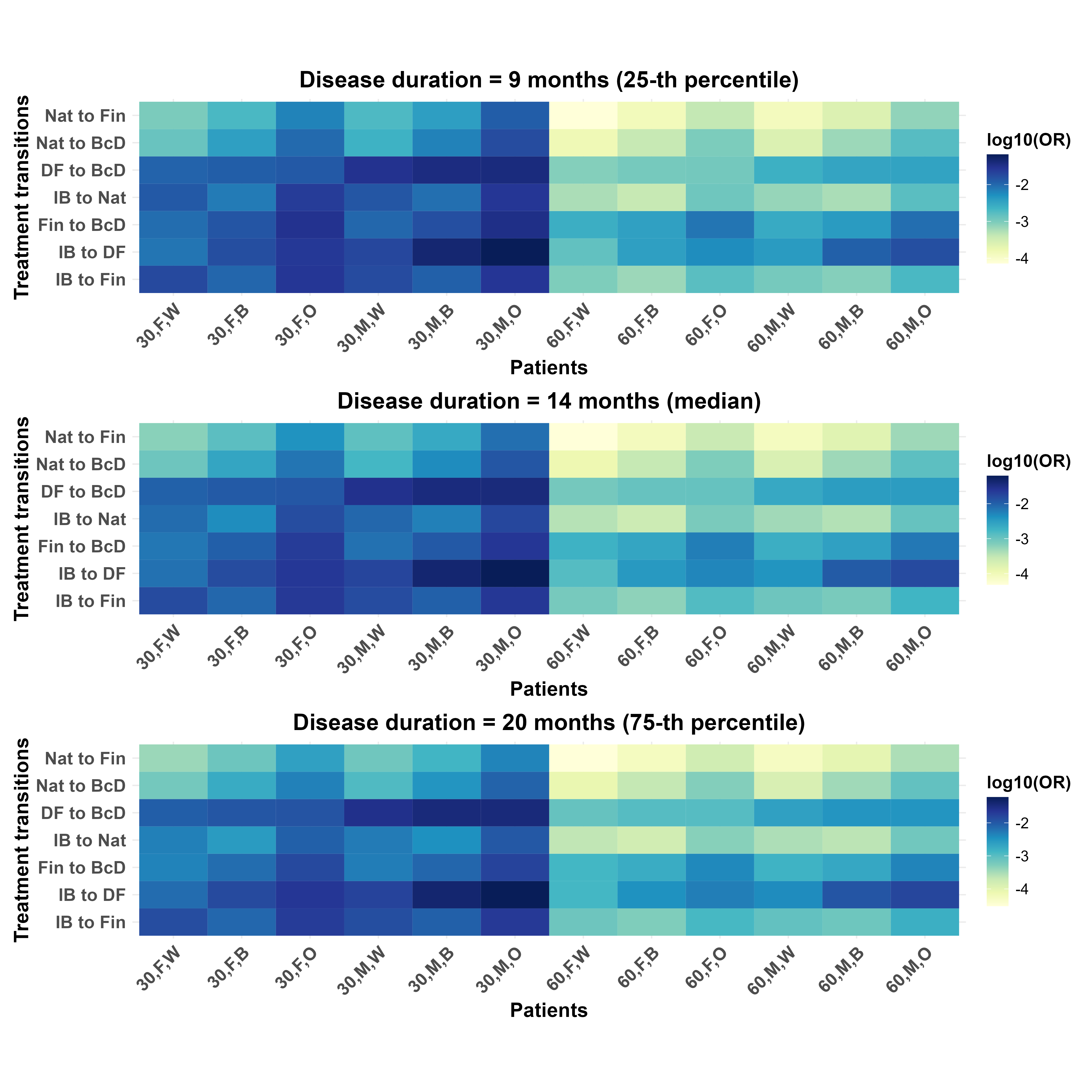
Figure 6: Odds ratios (OR) of transitioning to a different treatment versus continuing the same treatment for the top 7 most frequent MS DMT transitions (to a different one). The x-axis represents patients’ phenotypes: age, sex (M/F), and race (W = White, B = Black, O = Other). Plots are shown for all three quartiles (0.25, 0.5, 0.75) of disease duration.

6 Conclusion

In this article, we propose SMART-MC, a novel Markovian framework where initial state vectors and transition probabilities are modeled by subject-specific covariates, eventually unveiling the nature of the association of the covariates in modulating the transition probabilities, both in terms of direction and magnitude. SMART-MC also promptly addresses the issue with rare transitions, ultimately proposing a framework that not only avoids the extra computational burden of imposing sparsity but also uses such occurrences to its advantage by alleviating the burden to some extent, through avoiding estimating them as a function of covariates. This strategy ensures that the estimated transition probabilities across rare transitions exactly coincide with their empirical probabilities, while parsimoniously handling the $p>n$ issues that arise due to very low counts or non-existent occurrences of such rare transitions.

In order to handle the multi-modal likelihood arising in SMART-MC, we propose a Pattern Search (PS)-based global optimization technique, named MSCOR. Some of the attractive key features of MSCOR are noted as follows: (1) ability to escape local solutions, (2) parallelization using a number of threads linearly increasing with the dimension of the parameter space, (3) sparsity control, (4) automatic early termination capability while optimizing convex functions without prior knowledge, (5) non-convex detection. Further, MSCOR does not require the objective function to be differentiable; or even continuous. As the algorithm also does not require any adjustments based on objective functions, it can be used in its original form to optimize any non-differentiable or discontinuous objective function or those with non-closed forms. This makes MSCOR very powerful and versatile Black-box optimization tool on multiple spherically constrained spaces, being extensively relevant across all domains, far beyond its limiting role in this considered case-study.

Using SMART-MC, we propose a foundational strategy for studying how patient covariates are associated with their whole MS DMT sequence history, being the first of its kind. Our exploration led us to discover some key insights regarding how patient phenotypes like age at diagnosis, disease duration, gender, and race informing the likelihood of persistence with certain DMTs across diverse patient cohorts. In the future, this study can be generalized to handle sparse covariate effects, which may allow further incorporation of patients’ biomarker or neuroimaging within the model framework to close knowledge gaps regarding optimal treatment selection

Funding Statement

Dr. Xia is supported in part by NINDS R01NS098023 and R01NS124882.

SUPPLEMENTARY MATERIAL

Supplementary text:

Supplementary material is provided as a separate pdf document.

Code and data:

Codes for SMART-MC and MSCOR, including demos, are made available on Github (link).

References

- (1)
- Balusha & Morrow (2024) Balusha, A. & Morrow, S. (2024), ‘Multiple sclerosis in people over age 55’, Practical Neurology.
- Berger-Tal et al. (2014) Berger-Tal, O., Nathan, J., Meron, E. & Saltz, D. (2014), ‘The exploration-exploitation dilemma: A multidisciplinary framework’, PLoS ONE 9(4), e95693.
- Boggs & Tolle (1996) Boggs, P. & Tolle, J. (1996), ‘Sequential quadratic programming’, Acta Numerica pp. 1–52.
- Boyd & Vandenberghe (2004) Boyd, S. & Vandenberghe, L. (2004), Convex Optimization, Cambridge University Press.
- Branco et al. (2022) Branco, D., Martino, B., Esposito, A. et al. (2022), ‘Machine learning techniques for prediction of multiple sclerosis progression’, Soft Computing 26, 12041–12055.
- Brouwer et al. (2021) Brouwer et al. (2021), ‘Longitudinal machine learning modeling of ms patient trajectories improves predictions of disability progression’, Computer Methods and Programs in Biomedicine 208, 106180.
- Brown (2009) Brown, A. (2009), ‘Natalizumab in the treatment of multiple sclerosis’, Therapeutics and Clinical Risk Management 5(3), 585–594.
- Cantu-Paz & Goldberg (2000) Cantu-Paz, E. & Goldberg, D. (2000), ‘Efficient parallel genetic algorithms: theory and practice’, Computer Methods in Applied Mechanics and Engineering 186(2), 221–238.
- Carroll et al. (1997) Carroll, R., Fan, J., Gijbels, I. et al. (1997), ‘Generalized partially linear single-index models’, Journal of the American Statistical Association 92(438), 477–489.
- Casanova et al. (2022) Casanova, B., Quintanilla-Bordas, C. & Gascon, F. (2022), ‘Escalation vs. early intense therapy in multiple sclerosis’, J Pers Med 12(1), 119.
- Cavallo (2020) Cavallo, S. (2020), ‘Immune-mediated genesis of multiple sclerosis’, Journal of Translational Autoimmunity 3.
- Chi et al. (2007) Chi, Y., Paisley, W. & Carin, L. (2007), ‘Music analysis using hidden Markov mixture models’, IEEE Transactions on Signal Processing 55(11), 5209–5224.
- Coviello et al. (2014) Coviello, E., Chan, A. & Lanckriet, G. (2014), ‘Clustering hidden markov models with variational hem’, Journal of Machine Learning Research 15(22), 697–747.
- Das et al. (2022) Das et al. (2022), ‘Estimating the optimal linear combination of predictors using spherically constrained optimization’, BMC Bioinformatics 23(Suppl 3), 436.
- Das et al. (2023a) Das et al. (2023a), ‘Clustering sequence data with mixture markov chains with covariates using multiple simplex constrained optimization routine (msicor)’, Journal of Computational and Graphical Statistics 33(2), 379–392.
- Das et al. (2023b) Das et al. (2023b), ‘Utilizing biologic disease-modifying anti-rheumatic treatment sequences to subphenotype rheumatoid arthritis’, Arthritis Research and Therapy 25(1), 1–7.
- Das (2021) Das, P. (2021), ‘Recursive modified pattern search on high-dimensional simplex : A blackbox optimization technique’, The Indian Journal of Statistics - Sankhya B 83, 440–483.
- Das (2023) Das, P. (2023), ‘Black-box optimization on hyper-rectangle using recursive modified pattern search and application to ROC-based classification problem’, Sankhya B 85, 365–404.
- Das & Ghosal (2017) Das, P. & Ghosal, S. (2017), ‘Bayesian quantile regression using random b-spline series prior’, Computational Statistics & Data Analysis 109, 121–143.
- Dimitriouet al. (2023) Dimitriouet al. (2023), ‘Treatment of patients with multiple sclerosis transitioning between relapsing and progressive disease’, CNS Drugs 37, 69–92.
- Faissner & Gold (2019) Faissner, S. & Gold, R. (2019), ‘Oral therapies for multiple sclerosis’, Cold Spring Harbor Perspectives in Medicine 9(1), a032011.
- Fermi & Metropolis (1952) Fermi, E. & Metropolis, N. (1952), ‘Numerical solution of a minimum problem. los alamos unclassified report la–1492’, Los Alamos National Laboratory, Los Alamos, USA .
- Frascoli et al. (2022) Frascoli et al. (2022), ‘The dynamics of relapses during treatment switch in relapsing-remitting multiple sclerosis’, Journal of Theoretical Biology 541, 111091.
- Fraser (1957) Fraser, A. (1957), ‘Simulation of genetic systems by automatic digital computers’, Australian Journal of Biological Sciences 10, 484–491.
- Gelfand et al. (2017) Gelfand, J., Cree, B. & Hauser, S. (2017), ‘Ocrelizumab and other cd20+ b-cell-depleting therapies in multiple sclerosis’, Neurotherapeutics 14(4), 835–841.
- Geris (2012) Geris, L. (2012), Computational Modeling in Tissue Engineering, Springer.
- Goldschmidt & McGinley (2021) Goldschmidt, C. & McGinley, M. (2021), ‘Advances in the treatment of multiple sclerosis’, Neurologic Clinics 39(1), 21–33.
- Grand’Maison et al. (2018) Grand’Maison et al. (2018), ‘Sequencing of disease-modifying therapies for relapsing–remitting multiple sclerosis: a theoretical approach to optimizing treatment’, Current Medical Research and Opinion 34(8), 1419–1430.
- Gross & Corboy (2019) Gross, R. & Corboy, J. (2019), ‘Monitoring, switching, and stopping multiple sclerosis disease-modifying therapies’, Mult Scler Relat Disord. 25(3), 715–735.
- Gupta et al. (2016) Gupta, R., Kumar, R. & Vassilvitskii, S. (2016), ‘On mixtures of Markov chains’, Advances in neural information processing systems 29.
- Haan-Rietdijk et al. (2017) Haan-Rietdijk, S., Kuppens, P., Bergeman, C. et al. (2017), ‘On the use of mixed markov models for intensive longitudinal data’, Multivariate Behavioral Research 52(6), 747–767.
- Helske & Helske (2019) Helske, S. & Helske, J. (2019), ‘Mixture hidden Markov models for sequence data: the seqHMM package in R’, Journal of Statistical Software 88(3).
- Hoffmann et al. (2024) Hoffmann et al. (2024), ‘Preferences, adherence, and satisfaction: Three years of treatment experiences of people with multiple sclerosis’, Patient Preference and Adherence 18, 455–466.
- Iacobaeus et al. (2020) Iacobaeus, E., Arrambide, G., Amato, M. et al. (2020), ‘Aggressive multiple sclerosis (1): Towards a definition of the phenotype’, Multiple Sclerosis 26(9).
- Jamil & Yang (2013) Jamil, M. & Yang, X. (2013), ‘A literature survey of benchmark functions for global optimisation problems’, Int. J. Math. Model. 4(2).
- Kennedy & Eberhart (1995) Kennedy, J. & Eberhart, R. (1995), Particle swarm optimization, in ‘Proceedings of ICNN’95 - International Conference on Neural Networks’, Vol. 4, pp. 1942–1948.
- Kirkpatrick et al. (1983) Kirkpatrick, S., Gelatt, C. & Vecchi, M. (1983), ‘Optimization by simulated annealing’, Australian Journal of Biological Sciences 220(4598), 671–680.
- La-Mantia et al. (2016) La-Mantia, L., Pietrantonj, C. D., Rovaris, M. et al. (2016), ‘Interferons-beta versus glatiramer acetate for relapsing-remitting multiple sclerosis’, Cochrane Database Syst Rev 11(11), CD009333.
- Lan & Chan (2021) Lan, H. & Chan, A. (2021), ‘Hierarchical learning of hidden markov models with clustering regularization’, Proceedings of Machine Learning Research 161, 1628–1638.
- Lavori & Dawson (2014) Lavori, P. & Dawson, R. (2014), ‘Introduction to dynamic treatment strategies and sequential multiple assignment randomization’, Clinical Trials 11(4), 393–399.
- Lewis & Torczon (1999) Lewis, R. & Torczon, V. (1999), ‘Pattern search algorithms for bound constrained minimization’, SIAM Journal on Optimization 9(4), 1082–1099.
- Lewis & Torczon (2000) Lewis, R. & Torczon, V. (2000), ‘Pattern search algorithms for linearly constrained minimization’, SIAM Journal on Optimization 10(3), 917–941.
- Li et al. (2019) Li, T., Choi, M., Fu, K. et al. (2019), ‘Music sequence prediction with mixture hidden Markov models’, IEEE International Conference on Big Data pp. 6128–6132.
- Liang et al. (2022) Liang et al. (2022), ‘Temporal trends of multiple sclerosis disease activity: Electronic health records indicators’, Multiple Sclerosis and Related Disorders 57, 103333.
- Macaron et al. (2023) Macaron, G., Larochelle, C., Arbour, N. et al. (2023), ‘Impact of aging on treatment considerations for multiple sclerosis patients’, Frontiers in Neurology 14, 1197212.
-
MathWorks (2024)
MathWorks (2024), ‘Quick start parallel computing in matlab’.
Accessed: 2024-11-19.
https://www.mathworks.com/help/parallel-computing/ - Melnykov (2016) Melnykov, V. (2016), ‘Clickclust: An r package for model-based clustering of categorical sequences’, Journal of Statistical Software 74(9), 1–34.
- Nocedal & Wright (2006) Nocedal, J. & Wright, S. (2006), Numerical Optimization, Operations Research Series, 2nd edn, Springer.
- Paul et al. (2019) Paul, A., Comabella, M. & Gandhi, R. (2019), ‘Biomarkers in multiple sclerosis’, Cold Spring Harbor Perspectives in Medicine 9(3), a029058.
- Pinto et al. (2020) Pinto, M. F., Oliveira, H., Batista, S. et al. (2020), ‘Prediction of disease progression and outcomes in multiple sclerosis with machine learning’, Scientific Reports 10, 21038.
- Potra & Wright (2000) Potra, F. & Wright, S. (2000), ‘Interior-point methods’, Journal of Computational and Applied Mathematics 4, 281–302.
- Simpson et al. (2021) Simpson, A., Mowry, E. & Newsome, S. (2021), ‘Early aggressive treatment approaches for multiple sclerosis’, Current Treatment Options in Neurology 23(7), 19.
- Theil (1969) Theil, H. (1969), ‘A multinomial extension of the linear logit model’, International Economic Review 10, 251–259.
- Tibshirani (1996) Tibshirani, R. (1996), ‘Regression shrinkage and selection via the Lasso’, Journal of the Royal Statistical Society: Series B (Statistical Methodology) 58(1), 267–288.
- Torczon (1997) Torczon, V. (1997), ‘On the convergence of pattern search algorithms’, SIAM Journal on Optimization 7, 1–25.
- Urso et al. (2024) Urso, F., Abbruzzo, A., Chiodi, M. et al. (2024), ‘Model selection for mixture hidden markov models: an application to clickstream data’, Statistical Papers 65, 5797–5834.
- Wright (2005) Wright, M. (2005), ‘The interior-point revolution in optimization: History, recent developments, and lasting consequences’, Bulletin of American Mathematical Society 42, 39–56.
- Xia et al. (2013) Xia, Z., Secor, E., Chibnik, L. et al. (2013), ‘Modeling disease severity in multiple sclerosis using electronic health records’, Plos One 8(11), e78927.
- Zhang et al. (2023) Zhang et al. (2023), ‘Methods to balance the exploration and exploitation in differential evolution from different scales: A survey’, Neurocomputing 561, 126899.
- Zhao et al. (2017) Zhao, Y., Healy, C., Rotstein, D. et al. (2017), ‘Exploration of machine learning techniques in predicting multiple sclerosis disease course’, PLoS ONE 12(4), e0174866.
- Zhu & Xue (2006) Zhu, L. & Xue, L. (2006), ‘Empirical likelihood confidence regions in a partially linear single-index model’, Journal of the Royal Statistical Society: Series B 68(3), 549–570.