[b]Yoshinobu Kuramashi
Tensor renormalization group study of (1+1)-dimensional O(3) nonlinear sigma model with and without finite chemical potential
Abstract
We study (1+1)-dimensional O(3) nonlinear sigma model using the tensor renormalization group method with the infinite limit of the bond dimension . At the vanishing chemical potential , we investigate the von Neumann and Rényi types of entanglement entropies. The central charge is determined to be by using the asymptotic scaling properties of the entropies. We also examine the consistency between two entropies. In the finite density region with , where this model suffers from the sign problem in the standard Monte Carlo approach, we investigate the properties of the quantum phase transition. We determine the transition point and the critical exponent of the correlation length from the dependence of the number density in the thermodynamic limit. The dynamical critical exponent is also extracted from the scaling behavior of the temporal correlation length as a function of . This is the first successful calculation of the dynamical critical exponent with the TRG method.
1 Introduction
The basic idea of the tensor renormalization group (TRG) method 111In this paper, the “TRG method” or the “TRG approach” refers to not only the original numerical algorithm proposed by Levin and Nave [1] but also its extensions [2, 3, 4, 5, 6, 7, 8, 9, 10, 11, 12]. was originally proposed in the field of condensed matter physics in 2007 [1]. In the past decade the TRG method has been getting applied to the particle physics. Although the inital research target was focused on the phase transitions of two-dimensional (2) models, recent studies cover those for 4 models with the scalar, gauge and fermion fields [13, 14, 15, 10, 16, 17]. The particle physicists are attracted by the following characteristc features in the TRG method: (i) no sign problem, (ii) logarithmic computational cost on the system size, (iii) direct manipulation of the Grassmann variables, (iv) evaluation of the partition function or the path-integral itself. So far much attention has been paid to the featute (i) [3, 18, 19, 20, 21, 22, 23, 24, 25, 26, 14, 10, 27, 28, 29, 17, 30, 31],
In this report we investigate the (1+1) O(3) nonlinear sigma model (O(3) NLSM) with and without finite chemical potential. This model is massive and shares the property of asymptotic freedom with the (3+1) non-Abelian gauge theories so that it should be a good testbed before exploring to investigate the properties of QCD. At we measure the von Neumann and Rényi types of entanglement entropies taking advantage of the above feature (iv) [32]. The central charge is determined from the asymptotic scaling properties of the entanglement entropies. We also make a direct comparison of both entropies and discuss the consistency between them. At we perform a detailed study of the quantum phase transition, which is achieved thanks to the above features (i) and (ii) [33]. We determine the transition point , the critical exponent and the dynamical critical exponent , where and are theoretically expected based on the equivalence between the (1+1) O(3) NLSM at finite density and the integer-spin Heisenberg chain with a magnetic field [34, 35, 36, 37, 38].
2 Formulation
2.1 Tensor network representation
We consider the partition function of the O(3) NLSM with the chemical potential on a (1+1) lattice whose volume is . The temperature is given by . We set the lattice spacing unless necessary. A real three-component unit vector resides on the sites and satisfies the periodic boundary conditions (). The lattice action is defined as
| (1) |
where the spin and matrix are expressed as
| (5) | |||
| (9) |
with
| (10) |
Note that we introduce the chemical potential to the rotation between the second and third components.
The partition function and its measure are written as
| (11) | ||||
| (12) |
We discretize the integration (11) with the Gauss-Legendre quadrature [26] after changing the integration variables:
| (13) | |||||
| (14) |
We obtain
| (15) |
with , where and are - and -th roots of the -th Legendre polynomial on the site , respectively. denotes . is a 4-legs tensor defined by
| (16) |
The weight factor of the Gauss-Legendre quadrature is defined as
| (17) |
Throughout this report we employ . After performing the singular value decomposition (SVD) on , we obtain
| (18) |
where and denote unitary matrices and is a diagonal matrix with the largest singular values of in the descending order. We can obtain the tensor network representation of the O(3) NLSM on the site
| (19) |
Here the bond dimension of tensor is given by , which controls the numerical precision in the TRG method. The tensor network representation of the partition function is given by
| (20) |
In order to evaluate we employ the higher order tensor renormalization group (HOTRG) algorithm [2].
2.2 Correlation length and entanglement entropies
We evaluate the temporal correlation length with
| (21) |
where and is the largest and the second largest eigenvalues of the density matrix with the reduced single tensor obtained by HOTRG.
For calculation of the entanglement entropies we consider the system consisting of two subsystems A nad B with the same size of . The von Neumann entropy is obtained by
| (22) |
with , where denotes the trace restricted to the subsystem B. On the other hand, the Rényi entropy is defined by
| (23) |
with the th matrix power of . Both entropies are related by
| (24) |
3 Numerical results
3.1 Entanglement entropies with
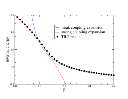
Before discussing the entanglement entropies, it may be instructive to show the results for the internal energy at obtained by the impure tensor method with [30]. In Fig. 1 we compare the TRG results with the strong and weak coupling expansions. In the strong coupling region we observe that our result show good consistency with the strong coupling expansion up to . On the other hand, the result starts to follow the weak coupling expansion curve around .
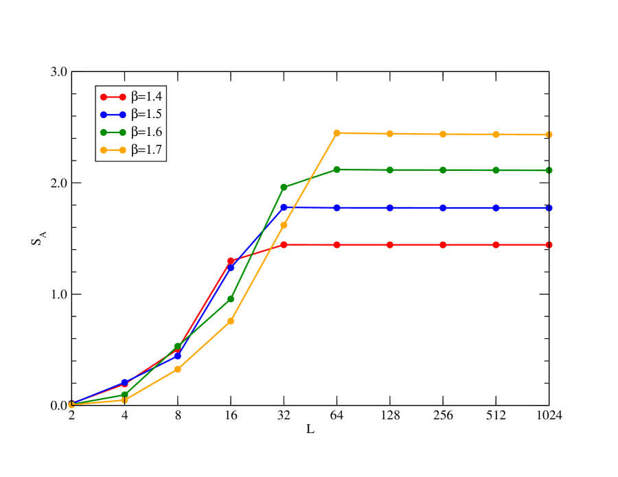
The density matrix is evaluated using HOTRG with the bond dimension . We choose , 1.5, 1.6 and 1.7 for the coupling constant to keep the condition , where the correlation length was precisely measured in Ref. [39]: , 11.09(2), 19.07(6) and 34.57(7) at , 1.5, 1.6 and 1.7, respectively.
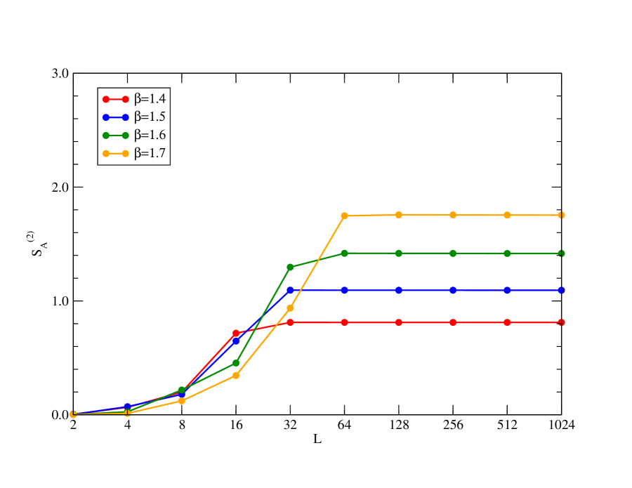
Figure 3 plots dependence of the von Neumann entropy at with , where is large enough to be regarded as the zero temperature limit. We observe that shows plateau behavior once the interval goes beyond the correlation length. As increases for larger , the plateau of starts at larger and its value is increased according to the theoretical expectation of with the central charge under the condition of [40]. For a comparative purpose we also plot the dependence of the 2nd-order Rényi entropy in Fig. 3. Both entropies show similar behaviors, though the plateau values of are smaller than those of according to the theoretical expectation [40].
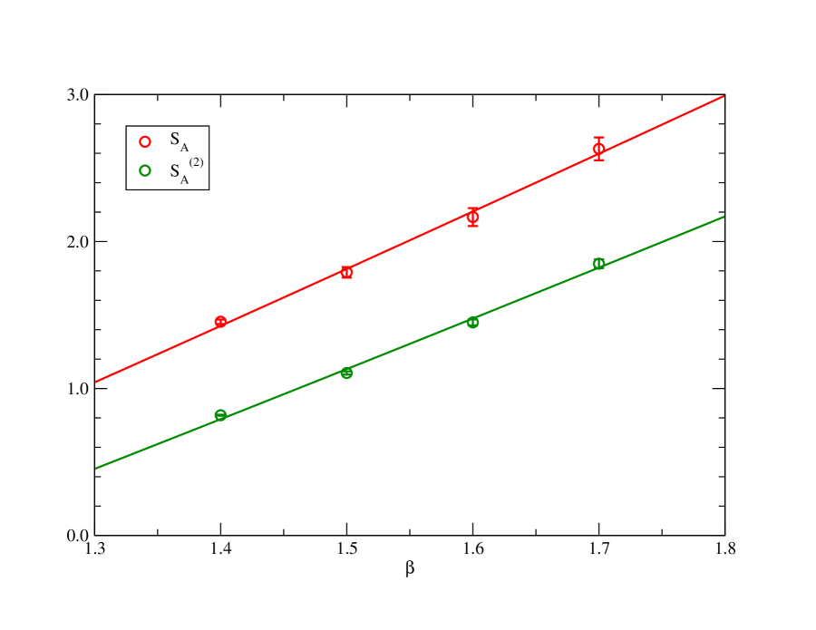
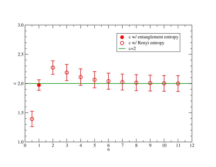
In Fig. 5 we show the dependence of and at , which are obtained by linear extrapolations in terms of to remove the finite effects. We extract the central charge by fitting the data with the following functions:
| (25) | |||||
| (26) |
with , where we use the perturbative dependence of . For the von Neumann entropy we obtain , which is consistent with obtained by the MPS method [41]. On the other hand, the value of extracted from the 2nd-order Rényi entropy is slightly larger than that from the von Neumann entropy. Repeating the same calculation for other th-order Rényi entropy we obtain the dependence of the central charge shown in Fig. 5. As increases the central charge seems to converges to and becomes consistent with determined from the von Neumann entropy. This convergence behavior may be explained by the fact that the largest eigenvalue in the density matrix, which is most presisely calculated, gives dominant contribution to the Rényi entropy as increases.
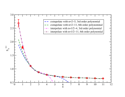
In Fig. 6 we plot the th-order Rényi entropy as a function of together with the von Neumann entropy at . Note that is obtained by the square root of the density matrix. We observe that rapidly increases toward in the region of . As a result, neither nor is a good approximation to the von Neumann entropy. Futhermore, this makes the precise extrapolation of with difficult as shown with blue and green broken lines in Fig. 6.
3.2 Quantum phase transition with
We evaluate the number density with the numerical differentiation of :
where the partition function is evaluated with the HOTRG algorithm with the bond dimensions , 130 and 135. We focus on in the case.
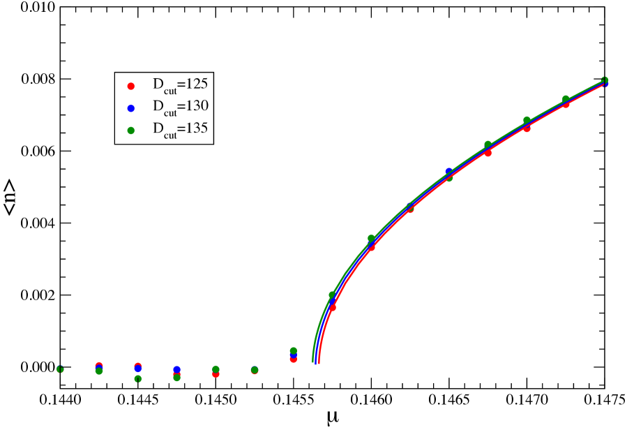
At the criticality of the second order phase tranasition the spatial correlation length should diverge as with the critical exponent. Since our model defined in Eq. (1) breakes the space-time symmetry due to the introduction of the chemical potential, the temporal correlation length should be deviated from and both are related by with the dynamical critical exponent.
Figure 8 plots the number density as a function of around the transition point on a lattice with . The volume is large enough to be regarded as the thermodynamic limit at zero temperature: and with the mass gap . Taking account of the slight dependence we apply the global fit to the data in the range of at assuming the function form of with , , and the fit parameters. The solid curves show the fit results with , , and , where the value of is consistent with the mass gap at obtained by a high precision Monte Carlo result [39].
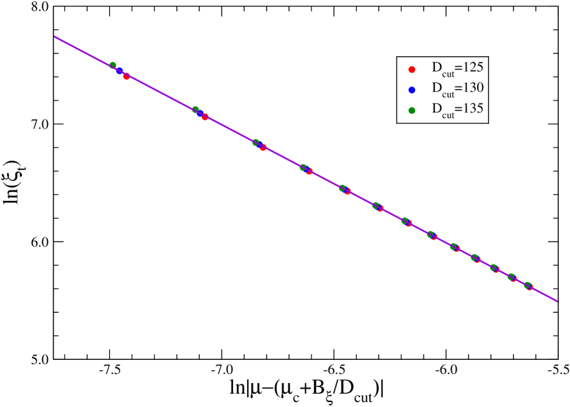
In Fig. 8 we show the results for the global fit of the temporal correlation length at employing the fit form of with . The solid curve, which shows fairly linear behavior, is drawn with the fit results of , and choosing . The relation with the use of gives the dynamical critical exponent . Our results of and are consistent with the theoretical expectation of and .
4 Summary
We have studied the (1+1) O(3) NLSM with the TRG method. At we calcuate the von Neumann and Rényi types of entanglement entropies. The central charge obtained from the asymptotic scaling behavior of the von Neumann entropy is , which is consistent with previously obtained with the MPS method. The direct comparison between both entropies implies that it may be difficult to estimate the von Neumann entropy at high precision from the extrapolation of higher-order Rényi etropies. We have also investigated the properties of the quantum phase transition with finite , which causes the sign problem in the Monte Carlo approach. We find the critical chemical potential at in the limit of , which is consistent with the mass gap at obtained in the Monte Carlo approach [39]. Our results for the critical exponent and the dynamical one also show consistency with the theoretical expectation of and . This is the first successful calculation of the dynamical critical exponent with the TRG method.
Acknowledgments
Numerical calculation for the present work was carried out with the supercomputers Cygnus and Pegasus under the Multidisciplinary Cooperative Research Program of Center for Computational Sciences, University of Tsukuba. We also used the supercomputer Fugaku provided by RIKEN through the HPCI System Research Project (Project ID: hp220203, hp230247). This work is supported in part by Grants-in-Aid for Scientific Research from the Ministry of Education, Culture, Sports, Science and Technology (MEXT) (Nos. 24H00214, 24H00940).
References
- [1] M. Levin and C. P. Nave, Tensor renormalization group approach to two-dimensional classical lattice models, Phys. Rev. Lett. 99 (2007) 120601, [cond-mat/0611687].
- [2] Z. Y. Xie, J. Chen, M. P. Qin, J. W. Zhu, L. P. Yang and T. Xiang, Coarse-graining renormalization by higher-order singular value decomposition, Phys. Rev. B 86 (2012) 045139, [1201.1144].
- [3] Y. Shimizu and Y. Kuramashi, Grassmann tensor renormalization group approach to one-flavor lattice Schwinger model, Phys. Rev. D90 (2014) 014508, [1403.0642].
- [4] G. Evenbly and G. Vidal, Tensor network renormalization, Phys. Rev. Lett. 115 (2015) 180405.
- [5] R. Sakai, S. Takeda and Y. Yoshimura, Higher order tensor renormalization group for relativistic fermion systems, PTEP 2017 (2017) 063B07, [1705.07764].
- [6] S. Yang, Z.-C. Gu and X.-G. Wen, Loop optimization for tensor network renormalization, Phys. Rev. Lett. 118 (2017) 110504.
- [7] M. Hauru, C. Delcamp and S. Mizera, Renormalization of tensor networks using graph independent local truncations, Phys. Rev. B97 (2018) 045111, [1709.07460].
- [8] D. Adachi, T. Okubo and S. Todo, Anisotropic Tensor Renormalization Group, Phys. Rev. B 102 (2020) 054432, [1906.02007].
- [9] D. Kadoh and K. Nakayama, Renormalization group on a triad network, 1912.02414.
- [10] S. Akiyama, Y. Kuramashi, T. Yamashita and Y. Yoshimura, Restoration of chiral symmetry in cold and dense Nambu–Jona-Lasinio model with tensor renormalization group, JHEP 01 (2021) 121, [2009.11583].
- [11] D. Adachi, T. Okubo and S. Todo, Bond-weighted tensor renormalization group, Phys. Rev. B 105 (2022) L060402, [2011.01679].
- [12] S. Akiyama, Bond-weighting method for the Grassmann tensor renormalization group, JHEP 11 (2022) 030, [2208.03227].
- [13] S. Akiyama, Y. Kuramashi, T. Yamashita and Y. Yoshimura, Phase transition of four-dimensional Ising model with higher-order tensor renormalization group, Phys. Rev. D100 (2019) 054510, [1906.06060].
- [14] S. Akiyama, D. Kadoh, Y. Kuramashi, T. Yamashita and Y. Yoshimura, Tensor renormalization group approach to four-dimensional complex theory at finite density, JHEP 09 (2020) 177, [2005.04645].
- [15] S. Akiyama, Y. Kuramashi and Y. Yoshimura, Phase transition of four-dimensional lattice theory with tensor renormalization group, Phys. Rev. D 104 (2021) 034507, [2101.06953].
- [16] S. Akiyama and Y. Kuramashi, Tensor renormalization group study of (3+1)-dimensional 2 gauge-Higgs model at finite density, JHEP 05 (2022) 102, [2202.10051].
- [17] S. Akiyama and Y. Kuramashi, Critical endpoint of (3+1)-dimensional finite density 3 gauge-Higgs model with tensor renormalization group, JHEP 10 (2023) 077, [2304.07934].
- [18] Y. Shimizu and Y. Kuramashi, Critical behavior of the lattice Schwinger model with a topological term at using the Grassmann tensor renormalization group, Phys. Rev. D90 (2014) 074503, [1408.0897].
- [19] H. Kawauchi and S. Takeda, Tensor renormalization group analysis of CP(-1) model, Phys. Rev. D93 (2016) 114503, [1603.09455].
- [20] H. Kawauchi and S. Takeda, Phase structure analysis of CP(N-1) model using Tensor renormalization group, PoS LATTICE2016 (2016) 322, [1611.00921].
- [21] L.-P. Yang, Y. Liu, H. Zou, Z. Xie and Y. Meurice, Fine structure of the entanglement entropy in the O(2) model, Phys. Rev. E 93 (2016) 012138, [1507.01471].
- [22] Y. Shimizu and Y. Kuramashi, Berezinskii-Kosterlitz-Thouless transition in lattice Schwinger model with one flavor of Wilson fermion, Phys. Rev. D97 (2018) 034502, [1712.07808].
- [23] S. Takeda and Y. Yoshimura, Grassmann tensor renormalization group for the one-flavor lattice Gross-Neveu model with finite chemical potential, PTEP 2015 (2015) 043B01, [1412.7855].
- [24] D. Kadoh, Y. Kuramashi, Y. Nakamura, R. Sakai, S. Takeda and Y. Yoshimura, Tensor network formulation for two-dimensional lattice = 1 Wess-Zumino model, JHEP 03 (2018) 141, [1801.04183].
- [25] D. Kadoh, Y. Kuramashi, Y. Nakamura, R. Sakai, S. Takeda and Y. Yoshimura, Investigation of complex theory at finite density in two dimensions using TRG, JHEP 02 (2020) 161, [1912.13092].
- [26] Y. Kuramashi and Y. Yoshimura, Tensor renormalization group study of two-dimensional U(1) lattice gauge theory with a term, JHEP 04 (2020) 089, [1911.06480].
- [27] S. Akiyama and Y. Kuramashi, Tensor renormalization group approach to (1+1)-dimensional Hubbard model, Phys. Rev. D 104 (2021) 014504, [2105.00372].
- [28] S. Akiyama, Y. Kuramashi and T. Yamashita, Metal–insulator transition in the (2+1)-dimensional Hubbard model with the tensor renormalization group, PTEP 2022 (2022) 023I01, [2109.14149].
- [29] K. Nakayama, L. Funcke, K. Jansen, Y.-J. Kao and S. Kühn, Phase structure of the CP(1) model in the presence of a topological -term, Phys. Rev. D 105 (2022) 054507, [2107.14220].
- [30] X. Luo and Y. Kuramashi, Tensor renormalization group approach to (1+1)-dimensional SU(2) principal chiral model at finite density, Phys. Rev. D 107 (2023) 094509, [2208.13991].
- [31] S. Akiyama and Y. Kuramashi, Tensor renormalization group study of (1 + 1)-dimensional U(1) gauge-Higgs model at = with Lüscher’s admissibility condition, JHEP 09 (2024) 086, [2407.10409].
- [32] X. Luo and Y. Kuramashi, Entanglement and Rényi entropies of (1+1)-dimensional O(3) nonlinear sigma model with tensor renormalization group, JHEP 03 (2024) 020, [2308.02798].
- [33] X. Luo and Y. Kuramashi, Quantum phase transition of (1+1)-dimensional O(3) nonlinear sigma model at finite density with tensor renormalization group, JHEP 11 (2024) 144, [2406.08865].
- [34] G. I. Dzhaparidze and A. A. Nersesyan, Magnetic-field phase transition in a one-dimensional system of electrons with attraction, JETP Lett. 27 (1978) 356.
- [35] V. L. Pokrovsky and A. L. Talapov, Ground state, spectrum, and phase diagram of two-dimensional incommensurate crystals, Phys. Rev. Lett. 42 (1979) 65.
- [36] H. J. Schulz, Critical behavior of commensurate-incommensurate phase transitions in two dimensions, Phys. Rev. B 22 (1980) 5274.
- [37] H. J. Schulz, Phase diagrams and correlation exponents for quantum spin chains of arbitrary spin quantum number, Phys. Rev. B 34 (1986) 6372.
- [38] I. Affleck, Theory of haldane-gap antiferromagnets in applied fields, Phys. Rev. B 41 (1990) 6697.
- [39] U. Wolff, Asymptotic Freedom and Mass Generation in the O(3) Nonlinear Model, Nucl. Phys. B 334 581.
- [40] P. Calabrese and J. L. Cardy, Entanglement entropy and quantum field theory, J. Stat. Mech. 0406 (2004) P06002, [hep-th/0405152].
- [41] F. Bruckmann, K. Jansen and S. Kühn, O(3) nonlinear sigma model in 1+1 dimensions with matrix product states, Phys. Rev. D 99 (2019) 074501, [1812.00944].