On the boundedness of Gross’ solution when the underlying distribution is bounded
On the boundedness of Gross’ solution to the planar Skorokhod embedding problem
Abstract
In this work, we investigate the problem of the boundedness of the Gross’ solutions of the planar Skorokhod embedding problem, where we show that the solution is bounded under some mild conditions on the underlying probability distribution.
Keywords and phrases: Planar Brownian motion, Skorokhod embedding problem
Mathematics Subject Classification (2010):
1 Introduction
In , the author R. Gross considered an interesting planar version of the Skorokhod problem [5], which was originally formulated in but in dimension one. For a concise survey of the one-dimensional 14 version, see [9]. The problem studied by Gross is as follows : Let be a non-degenerate probability distribution with zero mean and finite second moment. Is there a simply connected domain (containing the origin) such that, for a is a standard planar Brownian motion, then has the distribution ? Here is the exit time of the planar Brownian motion from . Gross provided an affirmative answer, offering an explicit construction of his solution. In addition, he showed that the underlying exit time has a finite average. One year later, Boudabra and Markowsky published two papers on the same problem [2, 1]. In the first one, the authors demonstrated that the problem is solvable for any non-degenerate distribution of a finite moment where . Furthermore, they provided a uniqueness criterion. The second paper provides a new category of domains that solve yet the Skorokhod embedding problem as well as a uniqueness criterion. As in [1], we shall keep using the terminology -domain to tag any simply connected domain solving the planar Skorokhod problem. As this manuscript deals with Gross’ solution, we confine ourselves to it, that is, a -domain means simply constructed by Gross’ technique. Let’s first summarize the geometric characteristics of the -domains generated by Gross’ method: :
-
•
is symmetric over the real line.
-
•
is -convex, i.e the segment joining any point of and its symmetric point over the real axis remains inside .
-
•
If then contains a vertical line segment, a half line, or a line.
-
•
If the support of the distribution has a gap from to then contains the vertical strip .
Note that the last two properties are universal, i.e they apply to any potential solution of the planar Skorokhod embedding problem. When it comes to boundedness, which is the focus of this note, any -domain is unbounded whenever the support of is either unbounded or contains a gap. Specifically, will be horizontally unbounded when the support of is unbounded, and vertically unbounded if there is a gap within the support of . Thus, two necessary conditions for obtaining a bounded -domain are the support of must be both bounded and connected (without gaps). Given these two assumptions, we will explore sufficient conditions on that lead a bounded -domain.
2 Tools and Results
We begin by outlining the ingredients of Gross’ technique to generate his -domain, a solution to the planar Skorokhod embedding problem.
The first one is the quantile function of defined by
| (1) |
where is the cumulative distribution function of , i.e , . In other words, is the pseudo-inverse of . When is increasing then simplifies to the standard inverse function. A handy feature of is that, when fed with uniformly distributed inputs in , it generates values sampling as . Note that if has a gap, say , then jumps by at . The “doubled periodic function” is extracted out of by setting
Remark that the function is even and non-decreasing.
The second ingredient is the periodic Hilbert transform, which will control the range of the projection of the -domain on the imaginary axis.
Definition 1.
The Hilbert transform of a - periodic function is defined by
where denotes the Cauchy principal value [3]. The role of is to absorb infinite limits near singularities in a certain sense. It is required for the Hilbert transform as the trigonometric function has poles at with . The Hilbert transform is a bounded operator on
for any . More precisely, we have
Theorem 2.
[3] If is in , then exists almost everywhere for . Furthermore, we have
| (2) |
for some positive constant .
The strong type estimate 2 fails to hold when , as becomes unbounded. For further details see [7, 4] [3, 6].
Now we illustrate Gross’ construction technique. He first generates the Fourier series expansion of :
where is the Fourier coefficient of . Note that there is no constant term due the fact that is assumed to be a centered probability distribution. Then he showed his cornerstone result, upon which the solution is built. More precisely
Theorem 3.
Using the conformal invariance principal of planar Brownian motion [8], Gross shows that , i.e the image of the under the action of , is a solution for the Skorokhod embedding problem. If one knows that then the boundary of his -domain is parameterized by
| (3) |
Now we state our first result. Let be a continuous probability distribution concentrated on an interval . Denote its density by . In particular, the quantile function simplifies to the standard inverse of . We state now our first theorem.
Theorem 4.
If is positive then the underlying -domain is bounded.
Proof.
As is assumed to be positive then is bounded on since
Let be a fixed number in . The Hilbert transform of is well defined as is bounded. By splitting the integral in into two parts, we have
| (4) |
Moreover, using a simple integration by parts, we obtain
| (5) |
Similarly,
| (6) |
By substituting (5) and (6) into (4), the Hilbert transform becomes
| (7) | ||||
∎
Now, since is differentiable at and , the first limit in (7) becomes
For the second limit in (7), observe that
On the other hand, the function is integrable on Then
is finite. Therefore,
is finite.
Remark 5.
The proof of Theorem 4 shows that is continuous as it is the convolution between an function and an function over .
The case where i.e at some point is inconclusive. The following two examples illustrate this fact. The first example generates a bounded -domain while the second example produces an unbounded one.
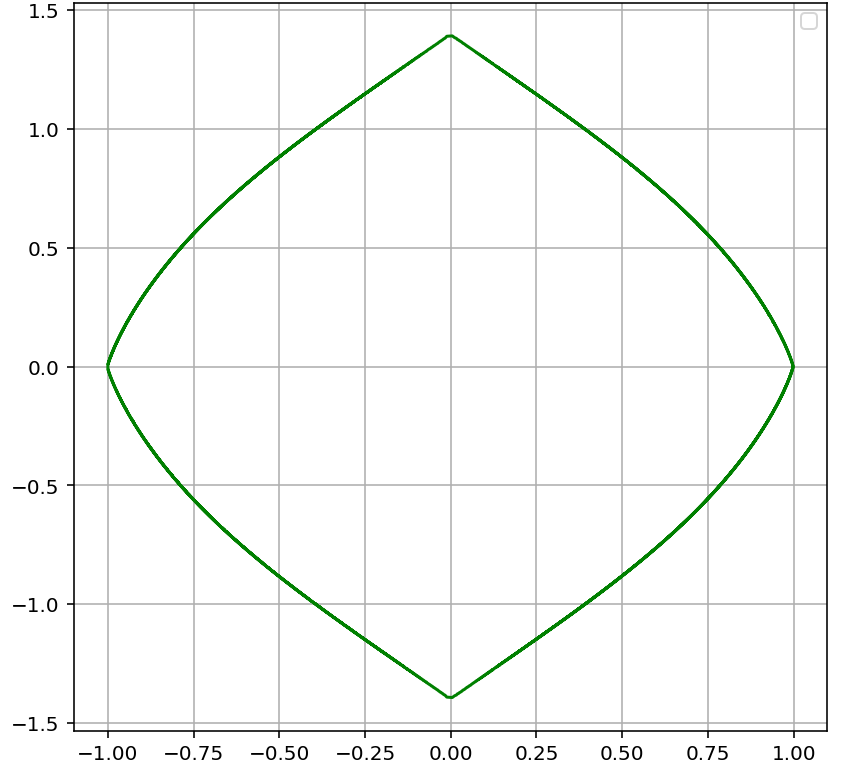
Example 6.
Let be the probability distribution given by the density
with being a non-negative parameter. The c.d.f of is
and thus
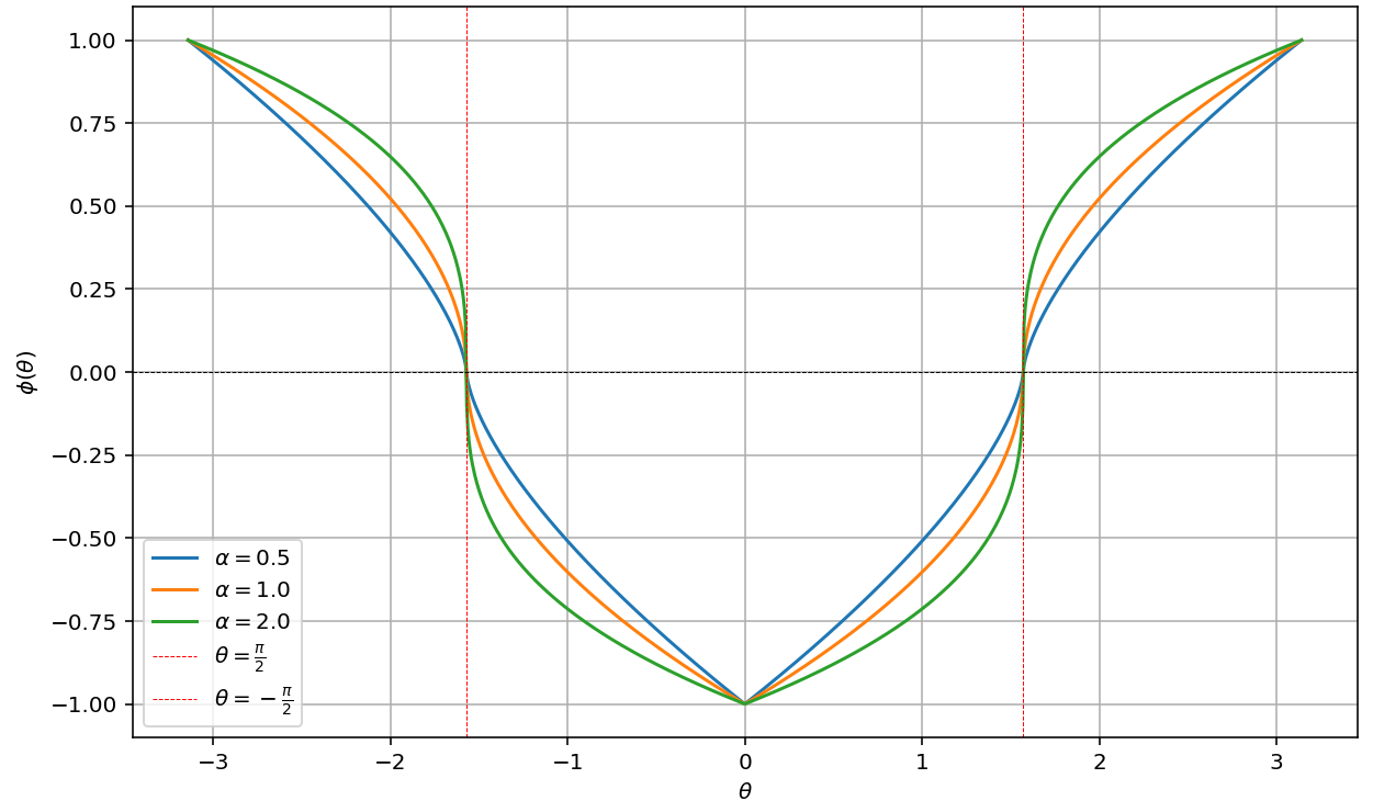
Now, as then we have the approximation:
| (8) |
As the R.H.S of 8 is integrable around , the function is also integrable. The case is similar. Hence
exists and is finite for all .
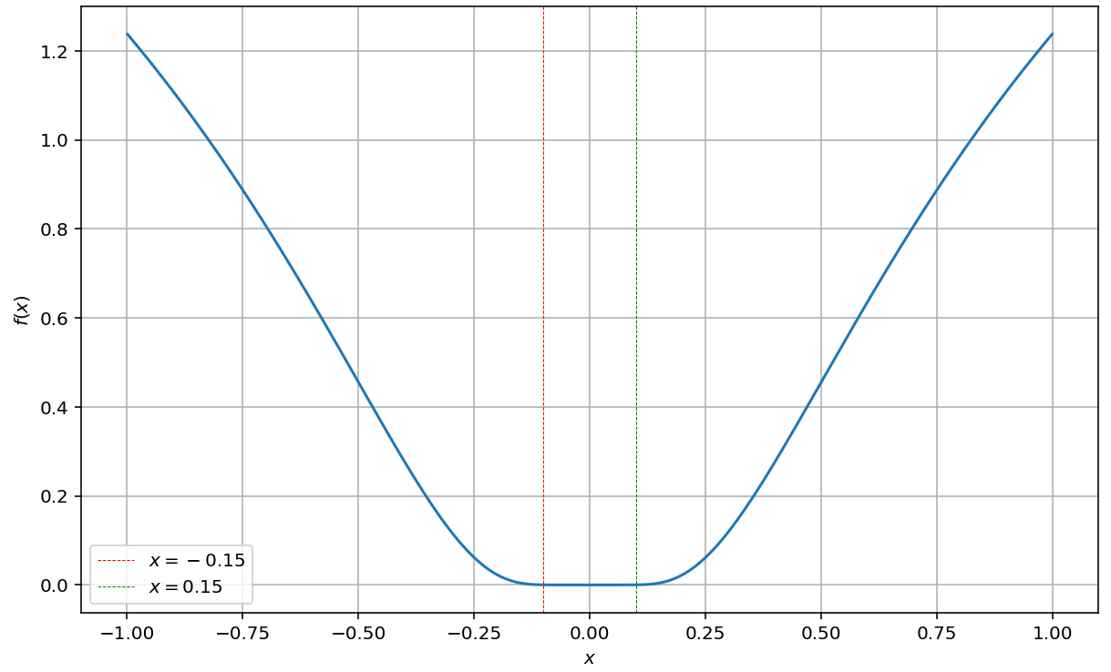
Example 7.
Before giving the example, we shall first provide the motivation behind. Theorem 4 says that any -domain is necessarily unbounded if is bounded. That is, if we want to seek a continuous distribution supported on an interval generating an unbounded domain, then necessarily its pdf must hit the -axis at some point . However hitting the value zero by is not enough as shown by the previous example. Even more, the previous example shows that if won’t do the job for any . So in order to boost the chance of getting an unbounded domain, must be too much flat around , i.e its graph looks like it is overlapped with the -axis at . In other words, we need such that
| (9) |
for any positive . Inspired by this analysis, we shall show that is a suitable candidate to generate an unbounded domain ( being the normalization constant).
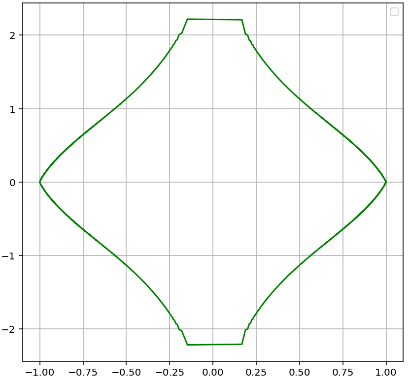
Since is symmetric, the associated cumulative distribution function takes the following form:
We have
An elementary property of inverses infers that
Hence
| (10) |
The R.H.S of 10 is not integrable around . Then we deduce that blows up, which infers that is unbounded.
3 Comments
In this work, we have investigated the problem of the boundedness of the -domains and found some sufficient conditions on the distribution to generate a bounded domain. In summary, in order to have a blow-up at some point , the graph of the quantile function must be too much steep. This includes the case of support with a gap. Assume that the support is for example, the quantile function will have a jump at the point . At this point, the derivative is the Dirac function, which is the most steep function ever. This explains the unboundedness of the corresponding -domain. An interesting question would be to discuss the necessity of such conditions, namely the flatness of the p.d.f, i.e can one find a distribution whose p.d.f satisfies 9 with a bounded -domai.
References
- [1] M. Boudabra and G. Markowsky. A new solution to the conformal Skorokhod embedding problem and applications to the Dirichlet eigenvalue problem. Journal of Mathematical Analysis and Applications, 491(2):124351, 2020.
- [2] M. Boudabra and G. Markowsky. Remarks on Gross’ technique for obtaining a conformal Skorohod embedding of planar Brownian motion. Electronic Communications in Probability, 2020.
- [3] P. Butzer and R. Nessel. Hilbert transforms of periodic functions. In Fourier Analysis and Approximation, pages 334–354. Springer, 1971.
- [4] P. L Duren. Theory of spaces. Courier Corporation, 2000.
- [5] R. Gross. A conformal Skorokhod embedding. Electronic Communications in Probability, 2019.
- [6] F. King. Hilbert transforms. Cambridge University Press Cambridge, 2009.
- [7] J D. McGovern. The Hilbert Transform. PhD thesis, 1980.
- [8] P. Mörters and Y. Peres. Brownian motion, volume 30. Cambridge University Press, 2010.
- [9] J. Obłój. The Skorokhod embedding problem and its offspring. Probability Surveys, pages 321 – 392, 2004.