Computing the Center of Uncertain Points on Cactus Graphs

Abstract

In this paper, we consider the (weighted) one-center problem of uncertain points on a cactus graph. Given are a cactus graph $G$ and a set of $n$ uncertain points. Each uncertain point has $m$ possible locations on $G$ with probabilities and a non-negative weight. The (weighted) one-center problem aims to compute a point (the center) $x^{*}$ on $G$ to minimize the maximum (weighted) expected distance from $x^{*}$ to all uncertain points. No previous algorithm is known for this problem. In this paper, we propose an $O(|G|+mn\log mn)$-time algorithm for solving it. Since the input is $O(|G|+mn)$, our algorithm is almost optimal.

1 Introduction

Problems on uncertain data have attracted an increasing amount of attention due to the observation that many real-world measurements are inherently accompanied with uncertainty. For example, the $k$-center model has been considered a lot on uncertain demands in facility locations [1, 19, 14, 22, 13, 3, 4, 16]. Due to the prevalence of tree-like graphs [10, 24, 5, 6, 11, 8] in facility locations, in this paper, we study the (weighted) one-center problem of uncertain points on a cactus-graph network.

Let $G=(V,E)$ be a cactus graph where any two cycles do not share edges. Every edge $e$ on $G$ has a positive length. A point $x=(u,v,t)$ on $G$ is characterized by being located at a distance of $t$ on edge $(u,v)$ from vertex $u$. Given any two points $p$ and $q$ on $G$, the distance $d(p,q)$ between $p$ and $q$ is defined as the length of their shortest path on $G$.

Let $\mathcal{P}$ be a set of $n$ uncertain points $P_{1},P_{2},\cdots,P_{n}$ on $G$. Each $P_{i}\in\mathcal{P}$ has $m$ possible locations (points) $p_{i1},p_{i2},\cdots,p_{im}$ on $G$. Each location $p_{ij}$ is associated with a probability $f_{ij}\geq 0$ for $P_{i}$ appearing at $p_{ij}$. Additionally, each $P_{i}\in\mathcal{P}$ has a weight $w_{i}\geq 0$.

Assume that all given points (locations) on any edge $e\in G$ are given sorted so that when we visit $e$, all points on $e$ can be traversed in order.

Consider any point $x$ on $G$. For any $P_{i}\in\mathcal{P}$, the (weighted) expected distance $\mathsf{E}\mathrm{d}(P_{i},x)$ from $P_{i}$ to $x$ is defined as $w_{i}\cdot\sum_{j=1}^{m}f_{ij}d(p_{ij},x)$. The center of $G$ with respect to $\mathcal{P}$ is defined to be a point $x^{*}$ on $G$ that minimizes the maximum expected distance $\max_{1\leq i\leq n}\mathsf{E}\mathrm{d}(P_{i},x)$. The goal is to compute center $x^{*}$ on $G$.

If $G$ is a tree network, then center $x^{*}$ can be computed in $O(mn)$ time by [21]. To the best of our knowledge, however, no previous work exists for this problem on cacti. In this paper, we propose an $O(|G|+mn\log mn)$-time algorithm for solving the problem where $|G|$ is the size of $G$. Note that our result matches the $O(|G|+n\log n)$ result [6] for the weighted deterministic case where each uncertain point has exactly one location.

1.1 Related Work

The deterministic one-center problem on graphs have been studied a lot. On a tree, the (weighted) one-center problem has been solved in linear time by Megiddo [18]. On a cactus, an $O(|G|+n\log n)$ algorithm was given by Ben-Moshe [6]. Note that the unweighted cactus version can be solved in linear time [17]. When $G$ is a general graph, the center can be found in $O(|E|\cdot|V|\log|V|)$ time [15], provided that the distance-matrix of $G$ is given. See [5, 23, 24] for variations of the general $k$-center problem.

When it comes to uncertain points, a few of results for the one-center problem are available. When $G$ is a path network, the center of $\mathcal{P}$ can be found in $O(mn)$ time [20]. On tree graphs, the problem can be addressed in linear time [22] as well. See [22, 13, 16] for the general $k$-center problem on uncertain points.

1.2 Our Approach

Lemma 5 shows that the general one-center problem can be reduced in linear time to a vertex-constrained instance where all locations of $\mathcal{P}$ are at vertices of $G$ and every vertex of $G$ holds at least one location of $\mathcal{P}$. Our algorithm focuses on solving the vertex-constrained version.

As shown in [10], a cactus graph is indeed a block graph and its skeleton is a tree where each node uniquely represents a cycle block, a graft block (i.e., a maximum connected tree subgraph), or a hinge (a vertex on a cycle of degree at least $3$) on $G$. Since center $x^{*}$ lies on an edge of a circle or a graft block on $G$, we seek for that block containing $x^{*}$ by performing a binary search on its tree representation $T$. Our $O(mn\log mn)$ algorithm requires to address the following problems.

We first solve the one-center problem of uncertain points on a cycle. Since each $\mathsf{E}\mathrm{d}(P_{i},x)$ is piece-wise linear but non-convex as $x$ moves along the cycle, our strategy is computing the local center of $\mathcal{P}$ on every edge. Based on our useful observations, we can resolve this problem in $O(mn\log mn)$ time with the help of the dynamic convex-hull data structure [2, 9].

Two more problems are needed to be addressed during the search for the node containing $x^{*}$. First, given any hinge node $h$ on $T$, the problem requires to determine if center $x^{*}$ is on $h$, i.e., at hinge $G_{h}$ $h$ represents, and otherwise, which split subtree of $h$ on $T$ contains $x^{*}$, that is, which hanging subgraph of $G_{h}$ on $G$ contains $x^{*}$. In addition, a more general problem is the center-detecting problem: Given any block node $u$ on $T$, the goal is to determine whether $x^{*}$ is on $u$ (i.e., on block $G_{u}$ on $G$), and otherwise, which split tree of the $H$-subtree of $u$ on $T$ contains $x^{*}$, that is, which hanging subgraph of $G_{u}$ contains $x^{*}$.

These two problems are more general problems on cacti than the tree version [21] since each $\mathsf{E}\mathrm{d}(P_{i},x)$ is no longer a convex function in $x$ on any path of $G$. We however observe that the median of any $P_{i}\in\mathcal{P}$ always fall in the hanging subgraph of a block whose probability sum of $P_{i}$ is at least $0.5$. Based on this, with the assistance of other useful observations and lemmas, we can efficiently solve each above problem in $O(mn)$ time.

Outline. In Section 2, we introduce some notations and observations. In Section 3, we present our algorithm for the one-center problem on a cycle. In Section 4, we discuss our algorithm for the problem on a cactus. In Section 5, we show how to linearly reduce any general case into a vertex-constrained case.

2 Preliminary

In the following, unless otherwise stated, we assume that our problem is the vertex-constrained case where every location of $\mathcal{P}$ is at a vertex on $G$ and every vertex holds at least one location of $\mathcal{P}$. Note that Lemma 5 shows that any general case can be reduced in linear time into a vertex-constrained case.

Some terminologies are borrowed from the literature [10]. A $G$-vertex is a vertex on $G$ not included in any cycle, and a hinge is one on a cycle of degree greater than $2$. A graft is a maximum (connected) tree subgraph on $G$ where every leaf is either a hinge or a $G$-vertex, all hinges are at leaves, and no two hinges belong to the same cycle. A cactus graph is indeed a block graph consisting of graft blocks and cycle blocks so that the skeleton of $G$ is a tree $T$ where for each block on $G$, a node is joined by an edge to its hinges. See Fig. 2 for an example.

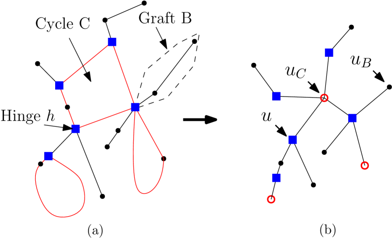
Figure 1: (a) Illustrating a cactus $G$ that consists of $3$ cycles, $5$ hinges (squares) and $6$ G-vertices (disks); (b) Illustrating $G$’s skeleton $T$ where circular and disk nodes represent cycles and grafts of $G$ (e.g., nodes $u$, $u_{C}$ and $u_{B}$ respectively representing hinge $h$, cycle $C$ and graft $B$ on $G$).

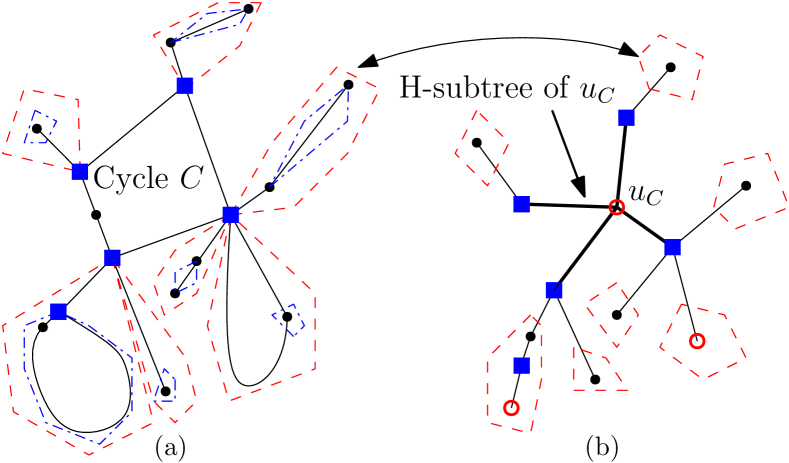
Figure 2: (a) Cycle $C$ on $G$ has $7$ split subgraphs (blue dash doted lines) and accordingly $7$ hanging subgraphs (red dashed lines); (b) on $T$, the H-subtree of node $u_{c}$ representing cycle $C$ has $7$ split subtrees each of which represents a distinct hanging subgraph of $C$ on $G$.

In fact, $T$ represents a decomposition of $G$ so that we can traverse nodes on $T$ in a specific order to traverse $G$ blocks by blocks in the according order. Our algorithm thus works on $T$ to compute center $x^{*}$. Tree $T$ can be computed by a depth-first-search on $G$ [10, 6] so that each node on $T$ is attached with a block or a hinge of $G$. We say that a node $u$ on $T$ is a block (resp., hinge) node if it represents a block (resp., hinge) on $G$. In our preprocessing work, we construct the skeleton $T$ with additional information maintained for nodes of $T$ to fasten the computation.

Denote by $G_{u}$ the block (resp., hinge) on $G$ of any block (resp., hinge) node $u$ on $T$. More specifically, we calculate and maintain the cycle circumstance for every cycle node on $T$. For any hinge node $h$ on $T$, $h$ is attached with hinge $G_{h}$ on $G$ (i.e., $h$ represents $G_{h}$). For each adjacent node $u$ of $h$, vertex $G_{h}$ also exists on block $G_{u}$ but with only adjacent vertices of $G_{u}$ (that is, there is a copy of $G_{h}$ on $G_{u}$ but with adjacent vertices only on $G_{u}$). We associate each adjacent node $u$ in the adjacent list of $h$ with vertex $G_{h}$ (the copy of $G_{h}$) on $G_{u}$, and also maintain the link from vertex $G_{h}$ on $G_{u}$ to node $h$.

Clearly, the size $|T|$ of $T$ is $O(mn)$ due to $|G|=O(mn)$. It is not difficult to see that all preprocessing work can be done in $O(mn)$ time. As a result, the following operations can be done in constant time.

1. Given any vertex $v$ on $G$, finding the node on $T$ whose block $v$ is on;

2. Given any hinge node $h$ on $T$, finding vertex $G_{h}$ on the block of every adjacent node of $h$ on $T$;

3. Given any block node $u$ on $T$, for any hinge on $G_{u}$, finding the hinge node on $T$ representing it.

Consider every hinge on the block of every block node on $T$ as an open vertex that does not contain any locations of $\mathcal{P}$. To be convenient, for any point $x$ on $G$, we say that a node $u$ on $T$ contains $x$ or $x$ is on $u$ if $x$ is on $G_{u}$. Note that $x$ may be on multiple nodes if $x$ is at a hinge on $G$. We say that a subtree on $T$ contains $x$ if $x$ is on one of its nodes.

Let $x$ be any point on $G$. Because $T$ defines a tree topology of blocks on $G$ so that vertices on $G$ can be traversed in some order. We consider computing $\mathsf{E}\mathrm{d}(P_{i},x)$ for all $1\leq i\leq n$ by traversing $T$. We have the following lemma. Note that it defines an order of traversing $G$, which is used in other operations of our algorithm.

Lemma 1

Given any point $x$ on $G$, $\mathsf{E}\mathrm{d}(P_{i},x)$ for all $1\leq i\leq n$ can be computed in $O(mn)$ time.

Proof

We create an array $A[1\cdots n]$ to maintain all $\mathsf{E}\mathrm{d}(P_{i},x)$ and initialize all as zero. Let $u_{x}$ be the block node on $T$ which contains $x$ and set it as the root of $T$. Clearly, $u_{x}$ as well as the corresponding point of $x$ on block $G_{u_{x}}$ can be obtained in $O(mn)$ time.

To compute $\mathsf{E}\mathrm{d}(P_{i},x)$ for all $1\leq i\leq n$, it suffices to traverse $G$ starting from $x$ to compute the distance of every location to $x$. To do so, we instead traverse $T$ in the pre-order from $u_{x}$: During the traversal, block $G_{u_{x}}$ of $u_{x}$ is first traversed in the pre-order from $x$ to compute the distance of its every location to $x$. For every other block node $u$, the block is traversed in the pre-order starting from the hinge (open-vertex) whose corresponding hinge node on $T$ is the parent of $u$. So is every hinge node on $T$.

More specifically, when we are visiting $G_{u_{x}}$, if $u_{x}$ is a cycle node then we traverse $G_{u_{x}}$ clockwise starting from $x$. During the traversal, for each vertex $v$, we first compute in constant time the distance $d(x,v)$; we next set $A[i]=A[i]+w_{i}\cdot f_{ij}\cdot d(x,v)$ for each location $p_{ij}$ at $v$ if $v$ is not a hinge; otherwise, we find in $O(1)$ time the hinge node $h$ on $T$ representing $v$ (i.e., $u_{x}$’s adjacent node), and set the distance $v$ on $h$ to $x$ as $d(x,v)$.

In the case of $G_{u_{x}}$ being a graft, we perform the pre-order traversal from $x$ to update $A[1\cdots n]$ in the above way. Otherwise, $G_{u_{x}}$ is a hinge and so $d(G_{u_{x}},x)=0$; we update $A[i]$ as the above for each location at $u_{x}$; we then set the distance $d(G_{u_{x}},x)=0$ for $G_{u_{x}}$ on the block of every adjacent node of $u_{x}$.

We continue our traversal on $T$ to visit $u_{x}$’s successors on $T$ in the pre-order to traverse their blocks. Suppose that we are visiting node $u$ on $T$. If $u$ is a hinge node, then its distance to $x$ can be known in constant time since hinge $G_{u}$ is an open vertex on the block of $u$’s parent node that has been visited. Consequently, we update $A[1\cdots n]$ as the above for every location $p_{ij}$ at $u$, and set the distance $d(G_{u},x)=0$ for $G_{u}$ on the block of every adjacent node of $u$.

Otherwise, we traverse block $G_{u}$ from the hinge (open vertex) represented by $u$’s parent hinge node $h$ on $T$, which can be find in $O(1)$ time. As the distance of $G_{h}$ to $x$ has been known, the distance from every vertex on $G_{u}$ to $x$ can be obtained in $O(1)$ time. We thus update $A[1\cdots n]$ for locations on $G_{u}$ similarly.

It follows that for any given point $x$ on $G$, values $\mathsf{E}\mathrm{d}(P_{i},x)$ of all $1\leq i\leq n$ can be obtained in $O(mn)$ time by performing a pre-order traversal on $T$.∎

We say that a point $x$ on $G$ is an articulation point if $x$ is on a graft block; removing $x$ generates several connected disjoint subgraphs; each of them is called a split subgraph of $x$; the subgraph induced by $x$ and one of its split subgraphs is called a hanging subgraph of $x$.

Similarly, any connected subgraph $G^{\prime}$ of $G$ has several split subgraphs caused by removing $G^{\prime}$, and each split subgraph with adjacent vertice(s) on $G^{\prime}$ contributes a hanging subgraph. See Fig. 2 (a) for an example.

Consider any uncertain point $P_{i}\in\mathcal{P}$. There exists a point $x^{*}_{i}$ on $G$ so that $\mathsf{E}\mathrm{d}(P_{i},x)$ reaches its minimum at $x=x^{*}_{i}$; point $x^{*}_{i}$ is called the median of $P_{i}$ on $G$. For any subgraph $G^{\prime}$ on $G$, we refer to value $\sum_{p_{ij}\in G^{\prime}}f_{ij}$ as $P_{i}$’s probability sum of $G^{\prime}$; we refer to value $w_{i}\cdot\sum_{p_{ij}\in G^{\prime}}f_{ij}\cdot d(p_{ij},x)$ as $P_{i}$’s (weighted) distance sum of $G^{\prime}$ to point $x$.

Notice that we say that median $x^{*}_{i}$ of $P_{i}$ (resp., center $x^{*}$) is on a hanging subgraph of a subgraph $G^{\prime}$ on $G$ iff $x^{*}_{i}$ (resp., $x^{*}$) is likely to be on that split subgraph of $G^{\prime}$ it contains. We have the following lemma.

Lemma 2

Consider any articulation point $x$ on $G$ and any uncertain point $P_{i}\in\mathcal{P}$.

1. If $x$ has a split subgraph whose probability sum of $P_{i}$ is greater than $0.5$, then its median $x_{i}^{*}$ is on the hanging subgraph including that split subgraph;

2. The point $x$ is $x_{i}^{*}$ if $P_{i}$’s probability sum of each split subgraph of $x$ is less than $0.5$;

3. The point $x$ is $x_{i}^{*}$ if $x$ has a split subgraph with $P_{i}$’s probability sum equal to $0.5$.

Proof

Let $G_{1}(x),\cdots,G_{s}(x)$ be all split subgraphs of $x$ on $G$. For claim $1$, we assume that $P_{i}$’s probability sum of $G_{1}(x)$ is larger than $0.5$. We shall show that $x^{*}_{i}$ is not likely to be on $G_{k}(x)$ for any $2\leq k\leq s$.

Consider any split subgraph $G_{k}(x)$ with $2\leq k\leq s$. Let $y$ be any point on $G_{k}(x)$. By the expected distance definition, we have the following.

$$\begin{split}\mathsf{E}\mathrm{d}(P_{i},y)&=w_{i}\sum_{p_{ij}\notin G_{k}(x)}f_{ij}[d(p_{ij},x)+d(x,y)]+w_{i}\sum_{p_{ij}\in G_{k}(x)}f_{ij}d(p_{ij},y)\\ &=w_{i}\sum_{p_{ij}\notin G_{k}(x)}f_{ij}d(p_{ij},x)+w_{i}\sum_{p_{ij}\notin G_{k}(x)}f_{ij}d(x,y)+w_{i}\sum_{p_{ij}\in G_{k}(x)}f_{ij}d(p_{ij},y)\\ &>w_{i}\sum_{p_{ij}\notin G_{k}(x)}f_{ij}d(p_{ij},x)+w_{i}\sum_{p_{ij}\in G_{k}(x)}f_{ij}[d(x,y)+d(p_{ij},y)]\\ &>w_{i}\sum_{p_{ij}\notin G_{k}(x)}f_{ij}d(p_{ij},x)+w_{i}\sum_{p_{ij}\in G_{k}(x)}f_{ij}d(p_{ij},x)\\ &=\mathsf{E}\mathrm{d}(P_{i},x)\end{split}$$

It follows that none of $G_{2}(x),\cdots,G_{s}(x)$ contain $x^{*}_{i}$ and $x^{*}_{i}$ is thus on the hanging subgraph $G_{1}(x)\cup\{x\}$. Therefore, both claims $1$ and $2$ hold.

For claim $3$, suppose that $P_{i}$’s probability sum of $G_{1}(x)$ is equal to $0.5$. To prove claim $3$, it is sufficient to prove $\mathsf{E}\mathrm{d}(P_{i},x)\leq\mathsf{E}\mathrm{d}(P_{i},y)$ for any point $y\in G_{1}(x)$. This can be verified similarly and we thus omit the details.∎

For any point $x\in G$, we say that $P_{i}$ is a dominant uncertain point of $x$ if $\mathsf{E}\mathrm{d}(P_{i},x)\geq\mathsf{E}\mathrm{d}(P_{j},x)$ for each $1\leq j\leq n$. Point $x$ may have multiple dominant uncertain points. Lemma 2 implies the following corollary.

Corollary 1

Consider any articulation point $x$ on $G$.

1. If $x$ has one dominant uncertain point whose median is at $x$, then center $x^{*}$ is at $x$;

2. If two dominant uncertain points have their medians on different hanging subgraphs of $x$, then $x^{*}$ is at $x$;

3. Otherwise, $x^{*}$ is on the hanging subgraph that contains all their medians.

Let $u$ be any block node on $T$; denote by $T^{H}_{u}$ the subtree on $T$ induced by $u$ and its adjacent (hinge) nodes; we refer to $T^{H}_{u}$ as the H-subtree of $u$ on $T$. Each hanging subgraph of block $G_{u}$ on $G$ is represented by a split subtree of $T^{H}_{u}$ on $T$. See Fig. 2 (b) for an example. Lemma 2 also implies the following corollary.

Corollary 2

Consider any block node $u$ on $T$ and any uncertain point $P_{i}$ of $\mathcal{P}$.

1. If the H-subtree $T^{H}_{u}$ of $u$ has a split subtree whose probability sum of $P_{i}$ is greater than $0.5$, then $x_{i}^{*}$ is on the split subtree of $T^{H}_{u}$;

2. If the probability sum of $P_{i}$ on each of $T^{H}_{u}$’s split subtree is less than $0.5$, then $x_{i}^{*}$ is on $u$ (i.e., block $G_{u}$ of $G$);

3. If $T^{H}_{u}$ has a split subtree whose probability sum of $P_{i}$ is equal to $0.5$, then $x_{i}^{*}$ is on that hinge node of $T^{H}_{u}$ that is adjacent to the split subtree.

Moreover, we have the following lemma.

Lemma 3

Given any articulation point $x$ on $G$, we can determine in $O(mn)$ time whether $x$ is $x^{*}$, and otherwise, which hanging subgraph of $x$ contains $x^{*}$.

Proof

Apply Lemma 1 to compute the array $A[1\cdots n]$ with $A[i]=\mathsf{E}\mathrm{d}(P_{i},x)$ in $O(mn)$ time, and then find the largest value $\delta$ of $A$ in $O(n)$ time. Create an array $F[1\cdots n]$ initialized as zero to store the probability sums of $x$’s dominant uncertain points on its each split subgraph, and another array $I[1\cdots n]$ initialized as $-1$ where $I[i]$ indicates $x$’s hanging subgraph containing $P_{i}$’s median $x_{i}^{*}$.

We proceed with determining which hanging subgraph of $x$ contains medians of $x$’s dominant uncertain points by traversing $T$. Let $u_{x}$ be the node on $T$ containing $x$, which can be found in $O(mn)$ time. Notice that $u_{x}$ is either a hinge node or a graft node on $T$. Let $u_{x}$ be the root of $T$.

On the one hand, $u_{x}$ is a graft node. Let $G^{1}_{u_{x}},\cdots,G^{s}_{u_{x}}$ be the split subgraphs of $x$ on block $G_{u_{x}}$ of $u_{x}$. Hence, $x$ has $s$ split subgraphs $G_{1}(x),\cdots,G_{s}(x)$ on $G$ and $G^{k}_{u_{x}}\in G_{k}(x)$ for each $1\leq k\leq s$. Specifically, for each $1\leq k\leq s$, denote by $v^{k}_{1},\cdots,v^{k}_{t}$ all hinges on $G^{k}_{u_{x}}$; since $G^{1}_{u_{x}},\cdots,G^{s}_{u_{x}}$ are disjoint, the subgraph induced by $G_{k}(x)/G^{k}_{u_{x}}$ and $\{u^{k}_{1},\cdots,u^{k}_{t}\}$ is represented by the union of subtrees on $T$ rooted at the corresponding hinge nodes $u^{k}_{1},\cdots,u^{k}_{t}$ of $v^{k}_{1},\cdots,v^{k}_{t}$.

To prove the lemma, it suffices to compute the probability sum of dominant uncertain points of $x$ on each $G_{k}(x)$. For each $G_{k}(x)$, we maintain a list $L_{k}$ to store $u^{k}_{1},\cdots,u^{k}_{t}$, which is empty initially. We then perform a traversal on $G_{k}(x)$ to compute the probability sum of uncertain points as follows.

We first traverse $G^{k}_{u_{x}}$: For each non-hinge vertex $v$ on $G^{k}_{u_{x}}$, for each location $p_{ij}$ at $v$, we set $F[i]=F[i]+f_{ij}$; we then check whether $F[i]>0.5$ and $A[i]=\delta$; if both yes, then $P_{i}$ is a dominant uncertain point at $x$ whose median is on $G_{k}(x)\cup\{x\}$, and thereby we set $I[i]=k$; otherwise, $P_{i}$ is not a dominant uncertain point and hence we continue our traversal on $G^{k}_{u_{x}}$. When a hinge vertex $v$ is currently encountered, we find in $O(1)$ time its corresponding hinge node on $T$, add it to $L_{k}$, and then continue our traversal on $G^{k}_{u_{x}}$.

Once we are done with traversing $G^{k}_{u_{x}}$, we continue to visit locations on the subgraph by $G_{k}(x)/G^{k}_{u_{x}}$ and $\{v^{k}_{1},\cdots,v^{k}_{t}\}$. In order to do so, we traverse the subtree of $T$ rooted at each hinge node of $L_{k}$. The traversal is similar to that in Lemma 1 and so the details are omitted.

Notice that after the above traversal on $G_{k}(x)$, we perform another traversal on $G_{k}(x)$ as the above, whereas during the traversal we reset $F[i]=0$ for each location $p_{ij}$ on $G_{k}(x)$. Clearly, the traversal on all $G_{k}(x)$ can be carried out in $O(mn)$ time.

To the end, we scan $I[1\cdots n]$ to determine which case of Corollary 1 $x$ falls into. More specifically, if there exist integers $i$ and $j$ with $1\leq i\neq j\leq n$ satisfying that $I[i],I[j]>0$ but $I[i]!=I[j]$, then two dominant uncertain points of $x$ have their medians on different hanging subgraphs of $x$ and so center $x^{*}$ must be at $x$; if $I[i]=-1$ for each $1\leq i\leq n$, $x^{*}$ is at $x$ as well; otherwise, only one hanging subgraph is found and it contains center $x^{*}$.

On the other hand, $u_{x}$ is a hinge node on $T$. Let $u_{1},\cdots,u_{s}$ be all adjacent (block) nodes of $u_{x}$ on $T$. Denote by $T_{u_{k}}$ the subtree rooted at $u_{k}$ on $T$. Clearly, for each $1\leq k\leq s$, the subgraph represented by $T_{u_{k}}$ excluding vertex $G_{u_{x}}$ is exactly $G_{k}(x)$. Since $G_{u_{x}}$ is an open vertex on $G_{u_{k}}$, traversing each $G_{k}(x)$ amounts to traversing $T_{u_{k}}$, and we add only $u_{k}$ into $L_{k}$ for each $1\leq k\leq s$. It follows that we traverse $T_{u_{k}}$ to visit locations on $G_{k}(x)$ to compute $F[1\cdots n]$ and $I[1\cdots n]$ for each $1\leq k\leq s$; finally, we scan $I[1\cdots n]$ to determine as the above case where center $x^{*}$ locates.

Therefore, the lemma holds.∎

Consider any hinge node $u$ on $T$. Lemma 3 implies the following corollary.

Corollary 3

Given any hinge node $u$ on $T$, we can determine in $O(mn)$ time whether $x^{*}$ is on $u$ (i.e., at hinge $G_{u}$ on $G$), and otherwise, which split subtree of $u$ contains $x^{*}$.

3 The One-Center Problem on a Cycle

In this section, we consider the one-center problem for the case of $G$ being a cycle. A general expected distance is considered: each $P_{i}\in\mathcal{P}$ is associated with a constant $c_{i}$ so that the (weighted) distance of $P_{i}$ to $x$ is equal to their (weighted) expected distance plus $c_{i}$. With a little abuse of notations, we refer to it as the expected distance $\mathsf{E}\mathrm{d}(P_{i},x)$ from $P_{i}$ to $x$.

Our algorithm focuses on the vertex-constrained version where every location is at a vertex on $G$ and every vertex holds at least one location. Since $G$ is a cycle, it is easy to see that any general instance can be reduced in linear time to a vertex-constrained instance.

Let $u_{1},u_{2},\cdots,u_{M}$ be the clockwise enumeration of all vertices on $G$, and $M\leq mn$. Let $l(G)$ be $G$’s circumstance. Every $u_{i}$ has a semicircular point $x_{i^{\prime}}$ with $d(u_{i},x_{i^{\prime}})=l(G)/2$ on $G$. Because sequence $x_{1^{\prime}},\cdots,x_{M^{\prime}}$ is in the clockwise order. $x_{1^{\prime}},\cdots,x_{M^{\prime}}$ can be computed in order in $O(mn)$ time by traversing $G$ clockwise.

Join these semicircular points $x_{1^{\prime}},\cdots,x_{M^{\prime}}$ to $G$ by merging them and $u_{1},\cdots,u_{M}$ in clockwise order; simultaneously, reindex all vertices on $G$ clockwise. Hence, a clockwise enumeration of all vertices on $G$ is generated in $O(mn)$ time. Clearly, the size $N$ of $G$ is now at most $2mn$. Given any vertex $u_{i}$ on $G$, there exists another vertex $u_{i^{c}}$ so that $d(u_{i},u_{i^{c}})=l(G)/2$. Importantly, $i^{c}=[{(i-1)}^{c}+1]\%N$ for $2\leq i\leq N$ and $1^{c}=(N^{c}+1)$.

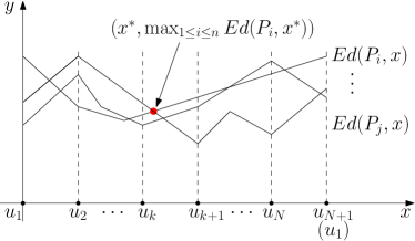
Figure 3: Consider $y=\mathsf{E}\mathrm{d}(P_{i},x)$ in $x,y$-coordinate system by projecting cycle $G$ onto $x$-axis; $\mathsf{E}\mathrm{d}(P_{i},x)$ of each $P_{i}\in\mathcal{P}$ is linear in $x$ on any edge of $G$; center $x^{*}$ is decided by the projection on $x$-axis of the lowest point on the upper envelope of all $y=\mathsf{E}\mathrm{d}(P_{i},x)$’s.

Let $x$ be any point on $G$. Consider the expected distance $y=\mathsf{E}\mathrm{d}(P_{i},x)$ in the $x,y$-coordinate system. We set $u_{1}$ at the origin and let vertices $u_{1},u_{2},\cdots,u_{N}$ $u_{N+1},\cdots,u_{2N}$ be on $x$-axis in order so that $u_{N+i}=u_{i}$. Denote by $x_{i}$ the $x$-coordinate of $u_{i}$ on $x$-axis. For $1\leq i<j\leq N$, the clockwise distance between $u_{i}$ and $u_{j}$ on $G$ is exactly value $x_{j}-x_{i}$ and their counterclockwise distance is equal to $x_{i+N}-x_{j}$.

As shall be analyzed below, each $\mathsf{E}\mathrm{d}(P_{i},x)$ is linear in $x\in[x_{s},x_{s+1}]$ for each $1\leq s\leq N$ but may be neither convex nor concave for $x\in[x_{1},x_{N+1}]$, which is different to the deterministic case [6]. See Fig. 3. Center $x^{*}$ is determined by the lowest point of the upper envelope of all $\mathsf{E}\mathrm{d}(P_{i},x)$ for $x\in[x_{1},x_{N+1}]$. Our strategy is computing the lowest point of the upper envelope on interval $[x_{s},x_{s+1}]$, i.e., computing the local center $x^{*}_{s,s+1}$ of $\mathcal{P}$ on $[x_{s},x_{s+1}]$, for each $1\leq s\leq N$. Center $x^{*}$ is obviously decided by the lowest one among all of them.

For each $1\leq s\leq N+1$, vertex $u_{s}$ has a semicircular point $x^{\prime}$ on $x$-axis with $x_{s}-x^{\prime}=l(G)/2$ and $x^{\prime}$ must be at a vertex on $x$-axis in that $u_{s}$ on $G$ has its semicircular point at vertex $u_{s^{c}}$. We still let $u_{s^{c}}$ be $u_{s}$’s semicircular point on $x$-axis. Clearly, for each $1\leq s\leq N$, $(s+1)^{c}=s^{c}+1$, and the semicircular point of any point in $[x_{s},x_{s+1}]$ lies in $[x_{s^{c}},x_{(s+1)^{c}]}]$. Indices $1^{c},2^{c},\cdots,(N+1)^{c}$ can be easily determined in order in $O(mn)$ time and so we omit the details.

Consider any uncertain point $P_{i}$ of $\mathcal{P}$. Because for any $1\leq s\leq N$, interval $[x_{s+1},x_{s+N}]$ contains all locations of $\mathcal{P}$ uniquely. We denote by $x_{ij}$ the $x$-coordinate of location $p_{ij}$ in $[x_{s+1},x_{s+N}]$; denote by $F_{i}(x_{s},x_{s^{c}})$ the probability sum of $P_{i}$’s locations in $[x_{s},x_{s^{c}}]$; let $D_{i}(x_{s+1},x_{s^{c}})$ be value $w_{i}\cdot\sum_{p_{ij}\in[x_{s+1},x_{s^{c}}]}f_{ij}x_{ij}$ and $D^{c}_{i}(x_{s^{c}+1},x_{s+N})$ be value $w_{i}\cdot\sum_{p_{ij}\in[x_{s^{c}+1},x_{s+N}]}f_{ij}(l(G)-x_{ij})$. Due to $F_{i}(x_{s+1},x_{s^{c}})+F_{i}(x_{s^{c}+1},x_{s+N})=1$, we have that $\mathsf{E}\mathrm{d}(P_{i},x)$ for $x\in[x_{s},x_{s+1}]$ can be formulated as follows.

$$\begin{split}\mathsf{E}\mathrm{d}(P_{i},x)&=c_{i}+w_{i}\sum_{p_{ij}\in[x_{s+1},x_{s^{c}}]}f_{ij}\cdot(x_{ij}-x)+w_{i}\sum_{p_{ij}\in[x_{s^{c}+1},x_{s+N}]}f_{ij}\cdot[l(G)-(x_{ij}-x)]\\ &=c_{i}+w_{i}(\sum_{p_{ij}\in[x_{s^{c}+1},x_{s+N}]}f_{ij}-\sum_{p_{ij}\in[x_{s+1},x_{s^{c}}]}f_{ij})\cdot x+w_{i}\sum_{p_{ij}\in[x_{s+1},x_{s^{c}}]}f_{ij}x_{ij}\\ &\ \ \ \ -w_{i}\sum_{p_{ij}\in[x_{s^{c}+1},x_{s+N}]}f_{ij}(l(G)-x_{ij})\\ &=w_{i}[1-2F_{i}(x_{s+1},x_{s^{c}})]\cdot x+c_{i}+D_{i}(x_{s+1},x_{s^{c}})-D^{c}_{i}(x_{s^{c}+1},x_{s+N})\end{split}$$

It turns out that each $\mathsf{E}\mathrm{d}(P_{i},x)$ is linear in $x\in[x_{s},x_{s+1}]$ for each $1\leq s\leq N$, and it turns at $x=x_{s}$ if $P_{i}$ has locations at points $u_{s}$, $u_{s^{c}}$, or $u_{s+N}$. Note that $\mathsf{E}\mathrm{d}(P_{i},x)$ may be neither convex nor concave. Hence, each $\mathsf{E}\mathrm{d}(P_{i},x)$ is a piece-wise linear function of complexity at most $m$ for $x\in[x_{1},x_{N+1}]$. It follows that the local center $x^{*}_{s,s+1}$ of $\mathcal{P}$ on $[x_{s},x_{s+1}]$ is decided by the $x$-coordinate of the lowest point of the upper envelope on $[x_{s},x_{s+1}]$ of functions $\mathsf{E}\mathrm{d}(P_{i},x)$’s for all $1\leq i\leq n$.

Consider the problem of computing the lowest points on the upper envelope of all $\mathsf{E}\mathrm{d}(P_{i},x)$’s on interval $[x_{s},x_{s+1}]$ for all $1\leq s\leq N$ from left to right. Let $L$ be the set of lines by extending all line segments on $\mathsf{E}\mathrm{d}(P_{i},x)$ for all $1\leq i\leq n$, and $|L|\leq mn$. Since the upper envelope of lines is geometric dual to the convex (lower) hull of points, the dynamic convex-hull maintenance data structure of Brodal and Jacob [9] can be applied to $L$ so that with $O(|L|\log|L|)$-time preprocessing and $O(|L|)$-space, our problem can be solved as follows.

Suppose that we are about to process interval $[x_{s},x_{s+1}]$. The dynamic convex-hull maintenance data structure $\Phi$ currently maintains the information of only $n$ lines caused by extending the line segment of each $\mathsf{E}\mathrm{d}(P_{i},x)$’s on $[x_{s-1},x_{s}]$. Let $\mathcal{P}_{s}$ be the subset of uncertain points of $\mathcal{P}$ whose expected distance functions turn at $x=x_{s}$. For each $P_{i}\in\mathcal{P}_{s}$, we delete from $\Phi$ function $\mathsf{E}\mathrm{d}(P_{i},x)$ for $x\in[x_{s-1},x_{s}]$ and then insert the line function of $\mathsf{E}\mathrm{d}(P_{i},x)$ on $[x_{s},x_{s+1}]$ into $\Phi$. After these $2|\mathcal{P}_{s}|$ updates, we compute the local center $x^{*}_{s,s+1}$ of $\mathcal{P}$ on $[x_{s},x_{s+1}]$ as follows.

Perform an extreme-point query on $\Phi$ in the vertical direction to compute the lowest point of the upper envelope of the $n$ lines. If the obtained point falls in $[x_{s},x_{s+1}]$, $x^{*}_{s,s+1}$ is of same $x$-coordinate as this point and its $y$-coordinate is the objective value at $x^{*}_{s,s+1}$; otherwise, it is to left of line $x=x_{s}$ (resp., to right of $x=x_{s+1}$) and thereby $x^{*}_{s,s+1}$ is of $x$-coordinate equal to $x_{s}$ (resp., $x_{s+1}$). Accordingly, we then compute the objective value at $x=x_{s}$ (resp., $x=x_{s+1}$) by performing another extreme-point query in direction $y=-x_{s}\cdot x$ (resp., $y=-x_{s+1}\cdot x$).

Note that $\mathcal{P}_{1}=\mathcal{P}$ for interval $[x_{1},x_{2}]$ and $\sum_{s=1}^{N}|P_{s}|=|L|\leq mn$. Since updates and queries each takes $O(\log|L|)$ amortized time, for each interval $[x_{s},x_{s+1}]$, we spend totally $O(|\mathcal{P}_{s}|\cdot\log|L|)$ amortized time on computing $x^{*}_{s,s+1}$. It implies that the time complexity for all updates and queries on $\Phi$ is $O(mn\log mn)$ time. Therefore, the total running time of computing the local centers of $\mathcal{P}$ on $[x_{s},x_{s+1}]$ for all $1\leq s\leq N$ is $O(mn\log mn)$ plus the time on determining functions $\mathsf{E}\mathrm{d}(P_{i},x)$ of each $P_{i}\in\mathcal{P}_{s}$ on $[x_{s},x_{s+1}]$ for all $1\leq s\leq N$.

We now present how to determine $\mathsf{E}\mathrm{d}(P_{i},x)$ of each $P_{i}\in\mathcal{P}_{s}$ in $x\in[x_{s},x_{s+1}]$ for all $1\leq s\leq N$. Recall that $\mathsf{E}\mathrm{d}(P_{i},x)=w_{i}\cdot[1-2F_{i}(x_{s+1},x_{s^{c}})]\cdot x+D_{i}(x_{s+1},x_{s^{c}})-D^{c}_{i}(x_{s^{c}+1},x_{s+N})+c_{i}$ for $x\in[x_{s},x_{s+1}]$. It suffices to compute the three coefficients $F_{i}(x_{s+1},x_{s^{c}})$, $D_{i}(x_{s+1},x_{s^{c}})$ and $D^{c}_{i}(x_{s^{c}+1},x_{s+N})$ for each $1\leq i\leq n$ and $1\leq s\leq N$.

We create auxiliary arrays $X[1\cdots n]$, $Y[1\cdots n]$ and $Z[1\cdots n]$ to maintain the three coefficients of $\mathsf{E}\mathrm{d}(P_{i},x)$ for $x$ in the current interval $[x_{s},x_{s+1}]$, respectively; another array $I[1\cdots n]$ is also created so that $I[i]=1$ indicates that $P_{i}\in\mathcal{P}_{s}$ for the current interval $[x_{s},x_{s+1}]$; we associate with $u_{s}$ for each $1\leq s\leq N$ an empty list $\mathcal{A}_{s}$ that will store the coefficients of $\mathsf{E}\mathrm{d}(P_{i},x)$ on $[x_{s},x_{s+1}]$ for each $P_{i}\in\mathcal{P}_{s}$. Initially, $X[1\cdots n]$, $Y[1\cdots n]$, and $Z[1\cdots n]$ are all set as zero, and $I[1\cdots n]$ is set as one due to $\mathcal{P}_{1}=\mathcal{P}$.

For interval $[x_{1},x_{2}]$, we compute $F_{i}(x_{2},x_{1^{c}})$, $D_{i}(x_{2},x_{1^{c}})$ and $D^{c}_{i}(x_{1^{c}+1},x_{N+1})$ for each $1\leq i\leq n$: for every location $p_{ij}$ in $[x_{2},x_{1^{c}}]$, we set $X[i]=X[i]+f_{ij}$ and $Y[i]=Y[i]+w_{i}\cdot f_{ij}\cdot x_{ij}$; for every location $p_{ij}$ in $[x_{1^{c}+1},x_{N+1}]$, we set $Z[i]=Z[i]+w_{i}\cdot(l(G)-x_{ij})$. Since $x_{1^{c}}$ is known in $O(1)$ time, it is easy to see that for all $P_{i}\in\mathcal{P}_{1}$, functions $\mathsf{E}\mathrm{d}(P_{i},x)$ for $x\in[x_{1},x_{2}]$ can be determined in $O(mn)$ time. Next, we store in list $\mathcal{A}_{1}$ the coefficients of $\mathsf{E}\mathrm{d}(P_{i},x)$ of all $P_{i}\in\mathcal{P}_{1}$ on $[x_{1},x_{2}]$: for each $I[i]=1$, we add tuples $(i,w_{i}\cdot X[i],c_{i}+Y[i]-Z[i])$ to $\mathcal{A}_{1}$ and then set $I[i]=0$. Clearly, list $\mathcal{A}_{1}$ for $u_{1}$ can be computed in $O(mn)$ time.

Suppose we are about to determine the line function of $\mathsf{E}\mathrm{d}(P_{i},x)$ on $[x_{s},x_{s+1}]$, i.e., coefficients $F_{i}(x_{s+1},x_{s^{c}})$, $D_{i}(x_{s+1},x_{s^{c}})$ and $D^{c}_{i}(x_{s^{c}+1},x_{s+N})$, for each $P_{i}\in\mathcal{P}_{s}$. Note that if $P_{i}$ has no locations at $u_{s}$, $u_{s^{c}}$ and $u_{s+N}$, then $P_{i}$ is not in $\mathcal{P}_{s}$; otherwise, $\mathsf{E}\mathrm{d}(P_{i},x)$ turns at $x=x_{s}$ and we need to determine $\mathsf{E}\mathrm{d}(P_{i},x)$ for $x\in[x_{s},x_{s+1}]$.

Recall that for $x\in[x_{s-1},x_{s}]$, $\mathsf{E}\mathrm{d}(P_{i},x)=c_{i}+w_{i}\cdot[1-2F_{i}(x_{s},x_{(s-1)^{c}})]\cdot x+D_{i}(x_{s},x_{(s-1)^{c}})-D^{c}_{i}(x_{(s-1)^{c}+1},x_{s-1+N})$. On account of $s^{c}=(s-1)^{c}+1$, for $x\in[x_{s},x_{s+1}]$, we have $F_{i}(x_{s+1},x_{s^{c}})=F_{i}(x_{s},x_{(s-1)^{c}})-F_{i}(x_{s},x_{s})+F_{i}(x_{s^{c}},x_{s^{c}})$, $D_{i}(x_{s+1},x_{s^{c}})=D_{i}(x_{s},x_{(s-1)^{c}})-D_{i}(x_{s},x_{s})+D_{i}(x_{s^{c}},x_{s^{c}})$, and $D^{c}_{i}(x_{s^{c}+1},x_{s+N})=D^{c}_{i}(x_{(s-1)^{c}+1},x_{s-1+N})-D^{c}_{i}(x_{s^{c}},x_{s^{c}})+D^{c}_{i}(x_{s+N},x_{s+N})$. Additionally, for each $1\leq i\leq n$, $\mathsf{E}\mathrm{d}(P_{i},x)$ on $[x_{s-1},x_{s}]$ is known, and its three coefficients are respectively in entries $X[i]$, $Y[i]$, and $Z[i]$. We can determine $\mathsf{E}\mathrm{d}(P_{i},x)$ of each $P_{i}\in\mathcal{P}_{s}$ on $[x_{s},x_{s+1}]$ as follows.

For each location $p_{ij}$ at $u_{s}$, we set $X[i]=X[i]-f_{ij}$, $Y[i]=Y[i]-w_{i}f_{ij}x_{ij}$ and $I[i]=1$; for each location $p_{ij}$ at $u_{s^{c}}$, we set $X[i]=X[i]+f_{ij}$, $Y[i]=Y[i]+w_{i}f_{ij}x_{ij}$, $Z[i]=Z[i]-w_{i}f_{ij}(l(G)-x_{ij})$ and $I[i]=1$; further, for each location $p_{ij}$ at $u_{s+N}$, we set $Z[i]=Z[i]+w_{i}f_{ij}(l(G)-x_{ij})$ and $I[i]=1$. Subsequently, we revisit locations at $u_{s}$, $u_{s^{c}}$ and $u_{s+N}$: for each location $p_{ij}$, if $I[i]=1$ then we add a tuple $(i,w_{i}\cdot X[i],c_{i}+Y[i]-Z[i])$ to $\mathcal{A}_{s}$ and set $I[i]=0$, and otherwise, we continue our visit.

For each $2\leq s\leq N$, clearly, functions $\mathsf{E}\mathrm{d}(P_{i},x)$ on $[x_{s},x_{s+1}]$ of all $P_{i}\in\mathcal{P}_{s}$ can be determined in the time linear to the number of locations at the three vertices $u_{s}$, $u_{s^{c}}$ and $u_{s+N}$. It follows that the time complexity for determining $\mathsf{E}\mathrm{d}(P_{i},x)$ of each $P_{i}\in\mathcal{P}_{s}$ for all $1\leq s\leq N$, i.e., computing the set $L$, is $O(mn)$; that is, the time complexity for determining $\mathsf{E}\mathrm{d}(P_{i},x)$ for each $P_{i}\in\mathcal{P}$ on $[x_{1},x_{N+1}]$ is $O(mn)$.

Combining all above efforts, we have the following theorem.

Theorem 3.1

The one-center problem of $\mathcal{P}$ on a cycle can be solved in $O(|G|+mn\log mn)$ time.

4 The Algorithm

In this section, we shall present our algorithm for computing the center $x^{*}$ of $\mathcal{P}$ on cactus $G$. We first give the lemma for solving the base case where a node of $T$, i.e., a block of $G$, is known to contain center $x^{*}$.

Lemma 4

If a node $u$ on $T$ is known to contain center $x^{*}$, then $x^{*}$ can be computed in $O(mn\log mn)$ time.

Proof

If $u$ is a hinge node, then $x^{*}$ is at its corresponding hinge $G_{u}$ on $G$, which can be obtained in $O(1)$ time, and we then return $G_{u}$ immediately.

Otherwise, block $G_{u}$ of node $u$ is a graft or a cycle. Let $u$ be the root of $T$; let $u_{1},\cdots,u_{s}$ be all child nodes of $u$, and each of them is a hinge node; vertices $G_{u_{1}},\cdots,G_{u_{s}}$ are (open) vertices on $G_{u}$. Denote by $T_{1}(u),\cdots,T_{s}(u)$ the split subtrees of $u$ on $T$; for each $1\leq k\leq s$, $T_{k}(u)$ is rooted at $u_{k}$, and let $G_{k}(u)$ be the subgraph on $G$ that $T_{k}(u)$ represents. Note that $T_{1}(u),\cdots,T_{s}(u)$ can be known in $O(mn)$ time.

On the one hand, $G_{u}$ is a graft and we then reduce our problem to an instance of the one-center problem with respect to a set $\mathcal{P}^{\prime}$ of $n$ uncertain points on a tree $G^{\prime}$ so that center $x^{*}$ can be computed in $O(mn)$ time by the algorithm [21] for tree graphs.

Initialize $G^{\prime}$ as $G_{u}$ and set $\mathcal{P}^{\prime}=\mathcal{P}$. To reduce our problem to a tree instance, we then do a pre-order traversal on $T_{k}(u)$ from $u_{k}$ to traverse $G_{k}(u)$. More specifically, for hinge node $u_{k}$, we reassign all locations at $u_{k}$ to vertex $G_{u_{k}}$ on $G^{\prime}$. For every other node $u^{\prime}$ on $T_{k}(u)$, as in Lemma 1, we traverse in the pre-order $G_{u^{\prime}}$ from the hinge represented by its parent node: for each vertex $v$, we first compute distance $d(G_{u_{k}},v)$ and next check if $v$ is an open vertex. If no, we join a new vertex $v^{\prime}$ into $G^{\prime}$, set the edge length between $v^{\prime}$ and $G_{u_{k}}$ on $G^{\prime}$ as $d(G_{u_{k}},v)$, and reassign all locations of $v$ to $v^{\prime}$; otherwise, we continue our traversal.

Clearly, traversing all $T_{k}(u)$’s in the above way takes $O(mn)$ time in total. Now, we obtain a tree $G^{\prime}$ of size $O(mn)$ and a set $\mathcal{P}^{\prime}$ of $n$ uncertain points where each $P_{i}\in\mathcal{P}^{\prime}$ has at most $m$ locations on $G^{\prime}$. It is not difficult to see that the center of $\mathcal{P}^{\prime}$ on $G^{\prime}$ corresponds a point on $G_{u}$ that is exactly the center of $\mathcal{P}$ on $G$. Consequently, center $x^{*}$ can be computed in $O(mn)$ time by the algorithm [21].

On the other hand, $G_{u}$ is a cycle and we then reduce our problem into a cycle case where a set $\mathcal{P}^{\prime}$ of $n$ uncertain points are on cycle $G^{\prime}$. Initially, we set $G^{\prime}$ as $G_{u}$, set $\mathcal{P}^{\prime}$ as $\mathcal{P}$, and assign a variable $c_{i}=0$ to each $P_{i}\in\mathcal{P}^{\prime}$. Similarly, we do a pre-order traversal on each $T_{k}(u)$ from $u_{k}$ to traverse $G_{k}(u)$. For $u_{k}$, we reassign $G_{u_{k}}$’s locations to the copy of $G_{u_{k}}$ on $G^{\prime}$. For every other node, we compute the distance $d(G_{u_{k}},v)$ for each vertex $v$ of the block; if $v$ is not an open vertex, then we reassign each location $p_{ij}$ at $v$ to $G_{u_{k}}$ on $G^{\prime}$, and set $c_{i}=c_{i}+w_{i}f_{ij}\cdot d(G_{u_{k}},v)$.

The above $O(mn)$-time traversal generates a cycle $G^{\prime}$ and a set $\mathcal{P}^{\prime}$ of $n$ uncertain points each with at most $m$ locations on $G^{\prime}$ and a constant $c_{i}$. We can see that computing $x^{*}$ of $\mathcal{P}$ on $G$ is equivalent to computing the center of $\mathcal{P}^{\prime}$ on $G^{\prime}$, which can be solved in $O(mn\log mn)$ time by Theorem 3.1.

Hence, the lemma holds.∎

Now we are ready to present our algorithm that performs a recursive search on $T$ to locate the node, i.e., the block on $G$, that contains center $x^{*}$. Once the node is found, Lemma 4 is then applied to find center $x^{*}$ in $O(mn\log mn)$ time.

On the tree, a node is called a centroid if every split subtree of this node has no more than half nodes, and the centroid can be found in $O(|T|)$ time by a traversal on the tree [15, 18].

We first compute the centroid $c$ of $T$ in $O(|T|)$ time. If $c$ is a hinge node, then we apply Corollary 3 to $c$, which takes $O(mn)$ time. If $x^{*}$ is on $c$, we then immediately return its hinge $G_{c}$ on $G$ as $x^{*}$; otherwise, we obtain a split subtree of $c$ on $T$ representing the hanging subgraph of hinge $G_{c}$ on $G$ that contains $x^{*}$.

On the other hand, $c$ is a block node. We then solve the center-detecting problem for $c$ that is to decide which split subtree of $c$’s H-subtree $T^{H}_{c}$ on $T$ contains $x^{*}$, that is, determine which hanging subgraph of block $G_{c}$ contains $x^{*}$. As we shall present in Section 4.1, the center-detecting problem can be solved in $O(mn)$ time. It follows that $x^{*}$ is either on one of $T^{H}_{c}$’s split subtrees or $T^{H}_{c}$. In the later case, since $G_{c}$ is represented by $T^{H}_{c}$, we can apply Lemma 4 to $c$ so that the center $x^{*}$ can be obtained in $O(mn\log mn)$ time.

In general, we obtain a subtree $T^{\prime}$ that contains center $x^{*}$. The size of $T^{\prime}$ is no more than half of $T$. Further, we continue to perform the above procedure recursively on the obtained $T^{\prime}$. Similarly, we compute the centroid $c$ of $T^{\prime}$ in $O(|T^{\prime}|)$ time; we then determine in $O(mn)$ time whether $x^{*}$ is on node $c$, and otherwise, find the subtree of $T^{\prime}$ containing $x^{*}$ but of size at most $|T^{\prime}|/2$.

As analyzed above, each recursive step takes $O(mn)$ time. After $O(\log mn)$ recursive steps, we obtain one node on $T$ that is known to contain center $x^{*}$. At this moment, we apply Lemma 4 to this node to compute $x^{*}$ in $O(mn\log mn)$ time. Therefore, the vertex-constrained one-center problem can be solved in $O(mn\log mn)$ time.

Recall that in the general case, locations of $\mathcal{P}$ could be anywhere on the given cactus graph rather than only at vertices. To solve the general one-center problem, we first reduce the given general instance to a vertex-constrained instance by Lemma 5, and then apply our above algorithm to compute the center. The proof for Lemma 5 is presented in Section 5.

Lemma 5

The general case of the one-center problem can be reduced to a vertex-constrained case in $O(|G|+mn)$ time.

Theorem 4.1

The one-center problem of $n$ uncertain points on cactus graphs can be solved in $O(|G|+mn\log mn)$ time.

4.1 The Center-Detecting Problem

Given any block node $u$ on $T$, the center-detecting problem is to determine which split subtree of $u$’s H-subtree $T^{H}_{u}$ on $T$ contains $x^{*}$, i.e., which hanging subgraph of block $G_{u}$ contains $x^{*}$. If $G$ is a tree, this problem can be solved in $O(mn)$ time [21]. Our problem is on cacti and a new approach is proposed below.

Let $G_{1}(u),\cdots,G_{s}(u)$ be all hanging subgraphs of block $G_{u}$ on $G$. For each $G_{k}(u)$, let $v_{k}$ be the hinge on $G_{k}(u)$ that connects its vertices with $G/G_{k}(u)$. $G_{1}(u),\cdots,G_{s}(u)$ are represented by split subtrees $T_{1}(u),\cdots,T_{s}(u)$ of $T^{H}_{u}$ on $T$, respectively.

Let $u$ be the root of $T$. For each $1\leq k\leq s$, $T_{k}(u)$ is rooted at a block node $u_{k}$, and hinge $v_{k}$ is an (open) vertex on block $G_{u_{k}}$. Additionally, the parent node of $u_{k}$ on $T$ is the hinge node $h_{k}$ on $T^{H}_{u}$ that represents $v_{k}$. Note that $h_{k}$ might be $h_{t}$ for some $1\leq t\neq k\leq s$. For all $1\leq k\leq s$, $T_{k}(u)$, $h_{k}$, and $v_{k}$ on block $G_{u_{k}}$ can be obtained in $O(mn)$ time via traversing subtrees rooted at $h_{1},\cdots,h_{s}$.

For each $1\leq k\leq s$, there is a subset $\mathcal{P}_{k}$ of uncertain points so that each $P_{i}\in\mathcal{P}_{k}$ has its probability sum of $G_{k}(u)/\{v_{k}\}$, i.e., $T_{k}(u)$, greater than $0.5$. Clearly, $\mathcal{P}_{i}\cap\mathcal{P}_{j}=\emptyset$ holds for any $1\leq i\neq j\leq s$.

Define $\tau(G_{k}(u))=\max_{P_{i}\in\mathcal{P}_{k}}\mathsf{E}\mathrm{d}(P_{i},v_{k})$. Let $\gamma$ be the largest value of $\tau(G_{k}(u))$’s for all $1\leq k\leq s$. We have the following observation.

Observation 1

If $\tau(G_{k}(u))<\gamma$, then center $x^{*}$ cannot be on $G_{k}(u)/\{v_{k}\}$; if $\tau(G_{r}(u))=\tau(G_{t}(u))=\gamma$ for some $1\leq r\neq t\leq s$, then center $x^{*}$ is on block $G_{u}$.

Proof

Let $G_{k}(u)$ be such hanging subgraph of $G_{u}$ with $\tau(G_{k}(u))<\gamma$. For each $1\leq r\neq k\leq s$, by Lemma 2, every uncertain point $P_{i}\in\mathcal{P}_{r}$ has $\mathsf{E}\mathrm{d}(P_{i},x)\geq\mathsf{E}\mathrm{d}(P_{i},v_{r})$ for any point $x\in G_{k}(u)$. Additionally, $\tau(G_{k}(u))<\gamma$. Hence, the dominant uncertain point at $v_{k}$ can not belong to $\mathcal{P}_{k}$. By Corollary 1, center $x^{*}$ cannot be on $G_{k}(u)/\{v_{k}\}$.

Suppose there are two subgraphs $G_{r}(u)$ and $G_{t}(u)$ with $\tau(G_{r}(u))=\tau(G_{t}(u))=\gamma$. To prove that $x^{*}$ is on $G_{u}$, it is sufficient to show that $x^{*}$ is on neither $G_{r}(u)/v_{r}$ nor $G_{t}(u)/v_{t}$. There are the two cases to consider.

If $v_{r}\neq v_{t}$, every $P_{i}\in\mathcal{P}_{r}$ has $\mathsf{E}\mathrm{d}(P_{i},v_{r})<\mathsf{E}\mathrm{d}(P_{i},v_{t})$ in that $P_{i}$’s probability sum of $G_{r}(u)$ is greater than $0.5$. Hence, the dominant uncertain point at $v_{t}$ cannot be in $\mathcal{P}_{t}$, and likewise, the dominant uncertain point at $v_{r}$ is not in $\mathcal{P}_{r}$. It implies that if $v_{r}\neq v_{t}$ then $x^{*}$ is on neither $G_{r}(u)/v_{r}$ nor $G_{t}(u)/v_{t}$.

Otherwise, $v_{r}$ is indeed $v_{t}$. If the dominant uncertain points of $v_{t}$ are in neither $\mathcal{P}_{r}$ nor $\mathcal{P}_{t}$, then $x^{*}$ cannot be on $G_{r}(u)/\{v_{r}\}\cup G_{t}(u)/\{v_{t}\}$. Otherwise, the objective value at $v_{t}$ is $\gamma$ due to $\tau(G_{r}(u))=\tau(G_{t}(u))=\gamma$. Hence, there are at least two dominant uncertain points at $v_{t}$: one in $\mathcal{P}_{r}$ determining $\tau(G_{r}(u))$ and the other in $\mathcal{P}_{t}$ determining $\tau(G_{t}(u))$. By Corollary 1, we have that $x^{*}$ is at $v_{t}$, namely, $x^{*}$ is on neither $G_{r}(u)/v_{r}$ nor $G_{t}(u)/v_{t}$.

The observation thus holds. ∎

Below, we first describe the approach for solving the center-detecting problem and then present how to compute values $\tau(G_{k}(u))$ for all $1\leq k\leq s$.

First, we compute $\gamma=\max_{k=1}^{s}\tau(G_{k}(u))$ in $O(s)$ time. We then determine in $O(s)$ time if there exists only one subgraph $G_{r}(u)$ with $\tau(G_{r}(u))=\gamma$. If yes, then center $x^{*}$ is on either $G_{r}(u)$ or $G_{u}$. Their only common vertex is $v_{r}$, and $v_{r}$ and its corresponding hinge $h_{r}$ on $T$ are known in $O(1)$ time. For this case, we further apply Corollary 3 to $h_{r}$ on $T$. If $x^{*}$ is at $v_{r}$ then we immediately return hinge $v_{r}$ on $G$ as the center; otherwise, we obtain the subtree on $T$ that represents the one containing $x^{*}$ among $G_{r}(u)$ and $G_{u}$, and return it.

On the other hand, there exist at least two subgraphs, e.g., $G_{r}(u)$ and $G_{t}(u)$, so that $\tau(G_{r}(u))=\tau(G_{t}(u))=\gamma$ for $1\leq r\neq t\leq s$. By Observation 1, $x^{*}$ is on $G_{u}$ and thereby node $u$ on $T$ is returned. Due to $s\leq mn$, we can see that all the above operations can be carried out in $O(mn)$ time.

To solve the center-detecting problem, it remains to compute $\tau(G_{k}(u))$ for all $1\leq k\leq s$. We first consider the problem of computing the distance $d(v_{k},x)$ for any given point $x$ and any given $v_{k}$ on $G$. We have the following result.

Lemma 6

With $O(mn)$-time preprocessing work, given any hinge $v_{k}$ and any point $x$ on $G$, the distance $d(v_{k},x)$ can be known in constant time.

Proof

For each $G_{k}(u)$ with $1\leq k\leq s$, as in Lemma 1, we do a pre-order traversal on $T_{k}(u)$ starting from its root $u_{k}$ to calculate the distance $d(v_{k},v)$ from every vertex $v$ on $G_{k}(u)$ to $v_{k}$, which can be done in $O(mn)$ time. Meanwhile, we associate every vertex $v$ on $G_{k}(u)/\{v_{k}\}$ with node $u_{k}$ on $T$ to indicate that $v$ uniquely belongs to $G_{k}(u)$. All these can be done in $O(mn)$ in total.

We proceed with traversing block $G_{u}$ to compute its inter-vertex distances for all vertices on $G_{u}$. If $u$ is a graft node, we pick any vertex on $G_{u}$ as its root $r$ and then preform a pre-order traversal on $G_{u}$ to compute the distance of each vertex to $r$. Further, we construct the lowest common ancestor data structure [7, 12] on $G_{u}$ so that with $O(|G_{u}|)$ preprocessing time and space, the lowest common ancestor of any two vertices on $G_{u}$ can be obtained in constant time.

Now, given are any two points $y$ and $z$ on $G_{u}$, and let $v_{y}$ (resp., $v_{z}$) be the closest vertex to $r$ that is adjacent to $y$ (resp., $z$). We first determine $v_{y}$ and $v_{z}$ in $O(1)$ time so that distances $d(y,r)$ and $d(z,r)$ can be known in $O(1)$ time. We then compute the lowest common ancestor $v^{\prime}$ of $v_{y}$ and $v_{z}$ by performing a constant-time query on the data structure. Due to $d(y,z)=d(y,r)+d(z,r)-2d(v^{\prime},r)$, $d(y,z)$ can be derived in constant time.

Otherwise, $u$ is a cycle node. In this situation, starting from any vertex $r$, we traverse $G_{u}$ clockwise to compute the clockwise distance of every vertex to $r$. For any points $y$ and $z$ on $G_{u}$, $d(y,z)$, equal to the minimum of their clockwise and counterclockwise distances, can be obtained in $O(1)$ time.

We now consider the problem of computing $d(v_{k},x)$ for any given $v_{k}$ and point $x$ on $G$. Let $(v,v^{\prime})$ be the edge that contains $x$ on $G$. Note that edge $(v,v^{\prime})$ is either on $G_{r}(u)$ for some $1\leq r\leq s$ or on $G_{u}$. So, there are only three cases to consider.

On the one hand, $v$ and $v^{\prime}$ are associated with the same node $u_{r}$ on $T$. Recall that hinge node $h_{r}$ is adjacent to $u_{r}$ and $u$ on $T$. It represents hinge $v_{r}$ on $G_{u}$, and $v_{r}$ is an open vertex on block $G_{u_{r}}$. So, edge $(v,v^{\prime})$ is on $G_{r}(u)/v_{r}$. We first obtain hinge $v_{r}$ on $G$ by $u_{r}$ in $O(1)$ time. If $v_{r}$ is exactly $v_{k}$, then $d(v_{k},x)$ can be obtained in $O(1)$ time since $d(v,v_{k})$ and $d(v^{\prime},v_{k})$ have been calculated ahead. Otherwise, hinges $v_{r}$ and $v_{k}$ are on block $G_{u}$. Since $d(v_{r},x)$ and $d(v_{r},v_{k})$ are obtained in $O(1)$ time, $d(v_{k},x)$, equal to their sum, can be known in constant time.

If only one of $v$ and $v^{\prime}$, say $v$, is associated with a node $u_{r}$ on $T$, then edge $(v,v^{\prime})$ is on $G_{r}(u)$ and $v^{\prime}$ is exactly hinge $v_{r}$ on $G_{u}$. Either $v_{r}$ is not $v_{k}$ (but both are on $G_{u}$), or $v_{r}=v_{k}$. For either case, distance $d(v_{k},x)$ can be known in constant time.

Otherwise, edge $(v,v^{\prime})$ is on $G_{u}$, i.e., neither of $v$ and $v^{\prime}$ are associated with any node on $T$. Clearly, distance $d(v_{k},x)$ can be known in constant time.

Therefore, the lemma holds. ∎

We now consider the problem of computing $\tau(G_{k}(u))$ for each $1\leq k\leq s$, which is solved as follows.

First, we determine the subset $\mathcal{P}_{k}$ for each $1\leq k\leq s$: Create auxiliary arrays $A[1\cdots n]$ initialized as zero and $B[1\cdots n]$ initialized as null. We do a pre-order traversal on $T_{k}(u)$ from node $u_{k}$ to compute the probability sum of each $P_{i}$ on $G_{k}(u)/{v_{k}}$. During the traversal, for each location $p_{ij}$, we add $f_{ij}$ to $A[i]$ and continue to check if $A[i]>0.5$. If yes, we set $B[i]$ as $u_{k}$, and otherwise, we continue our traversal on $T_{k}(u)$. Once we are done, we traverse $T_{k}(u)$ again to reset $A[i]=0$ for every location $p_{ij}$ on $T_{k}(u)$. Clearly, $B[i]=u_{k}$ iff $P_{i}\in\mathcal{P}_{k}$. After traversing $T_{1}(u),\cdots,T_{s}(u)$ as the above, given any $1\leq i\leq n$, we can know to which subset $P_{i}$ belongs by accessing $B[i]$.

To compute $\tau(G_{k}(u))$ for each $1\leq k\leq s$, it suffices to compute $\mathsf{E}\mathrm{d}(P_{i},v_{k})$ for each $P_{i}\in\mathcal{P}_{k}$. In details, we first create an array $L[1\cdots n]$ to maintain values $\mathsf{E}\mathrm{d}(P_{i},v_{k})$ of each $P_{i}\in\mathcal{P}_{k}$ for all $1\leq k\leq s$. We then traverse $G$ directly to compute values $\mathsf{E}\mathrm{d}(P_{i},v_{k})$. During the traversal on $G$, for each location $p_{ij}$, if $B[i]$ is $u_{k}$, then $P_{i}$ is in $\mathcal{P}_{k}$. We continue to compute in constant time the distance $d(p_{ij},v_{k})$ by Lemma 6, and then add value $w_{i}\cdot f_{ij}\cdot d(p_{ij},v_{k})$ to $L[i]$. It follows that in $O(mn)$ time we can compute values $\mathsf{E}\mathrm{d}(P_{i},v_{k})$ of each $P_{i}\in\mathcal{P}_{k}$ for all $1\leq k\leq s$.

With the above efforts, $\tau(G_{k}(u))$ for all $1\leq k\leq s$ can be computed by scanning $L[1\cdots n]$: Initialize each $\tau(G_{k}(u))$ as zero. For each $L[i]$, supposing $B[i]$ is $u_{k}$, we set $\tau(G_{k}(u))$ as the larger of $\tau(G_{k}(u))$ and $L[i]$. Otherwise, either $L[i]=0$ or $B[i]$ is null, and hence we continue our scan. These can be carried out in $O(n)$ time.

In a summary, with $O(mn)$-preprocessing work, values $\tau(G_{k}(u))$ for all $1\leq k\leq s$ can be computed in $O(mn)$ time. Once values $\tau(G_{k}(u))$ are known, as the above stated, the center-detecting problem for any given block node $u$ on $T$ can be solved in $O(mn)$ time. The following lemma is thus proved.

Lemma 7

Given any block node $u$ on $T$, the center-detecting problem can be solved in $O(mn)$ time.

5 Reducing the General Case to the Vertex-Constrained Case

In this section, we present how to reduce the general case to a vertex-constrained case. In the following, we say that a vertex on $G$ is empty if there are no locations at the vertex.

Let $C$ be a cycle on $G$ of only two hinges where all other vertices are empty. Denote by $\pi$ the shorter path on $C$ between two hinges. If the length of $\pi$ is $l(C)/2$, then let $\pi$ be any of their clockwise and counterclockwise paths on $C$. The following observation helps reduce the size of $G$.

Observation 2

If center $x^{*}$ is on $C$, $x^{*}$ must be on $\pi$.

Proof

Since only two hinges are on $C$ and all other vertices are empty, every empty non-hinge vertex on $C$ can be removed from $C$. On purpose of analysis, we assume that $C$ contains only two hinges.

Suppose that $\pi$ is the counterclockwise path between two hinges longer than their clockwise path. Join the semicircular point of every hinge as a new vertex to $C$. Let $\{u_{1},u_{2},u_{3},u_{4}\}$ be their clockwise enumerations starting from hinge $u_{1}$. We thus have the following properties: $u_{4}$ is the other hinge; $u_{2}$ must be $u_{4}$’s semicircular point; $u_{3}$ must be that of $u_{1}$.

Removing $C$ except for $u_{1},u_{4}$ generates two disjoint subgraphs $G_{1}$ and $G_{4}$ where $u_{1}$ is on $G_{1}$ and $u_{4}$ is on $G_{4}$ (and which are not hanging subgraphs of $C$). All $mn$ locations of $\mathcal{P}$ are on $G_{1}\cup G_{4}$. Denote by $\mathcal{P}_{1}$ the subset of all uncertain points in $\mathcal{P}$ each with its probability sum of $G_{1}$ at least $0.5$, and by $\mathcal{P}_{2}$ the subset of uncertain points each with its probability sum of $G_{4}$ at least $0.5$. Hence, $\mathcal{P}_{1}\cup\mathcal{P}_{2}=\mathcal{P}$.

Let $x$ be any point on $C$. Consider function $\mathsf{E}\mathrm{d}(P_{i},x)$ of each $P_{i}\in\mathcal{P}$ with respect to $x$. It is easy to see that each $\mathsf{E}\mathrm{d}(P_{i},x)$ linearly increases as $x$ moves clockwise from $u_{1}$ to $u_{2}$ along edge $(u_{1},u_{2})$, and so does it as $x$ moves counterclockwise from $u_{4}$ to $u_{3}$ along edge $(u_{4},u_{3})$. This means that the objective value at any point of $(u_{1},u_{2})/\{u_{1}\}$ (resp., $(u_{4},u_{3})/\{u_{4}\}$) is larger than that at $u_{1}$ (resp., $u_{4}$). Thus, center $x^{*}$ is on neither $(u_{1},u_{2})/\{u_{1}\}$ nor $(u_{4},u_{3})/\{u_{4}\}$.

What’s more, for each $P_{r}\in\mathcal{P}_{1}$, function $\mathsf{E}\mathrm{d}(P_{r},x)$ monotonically increases from $\mathsf{E}\mathrm{d}(P_{r},u_{2})$ to $\mathsf{E}\mathrm{d}(P_{r},u_{3})$ as $x$ moves clockwise from $u_{2}$ to $u_{3}$ along edge $(u_{2},u_{3})$. It monotonically increases as well from $\mathsf{E}\mathrm{d}(P_{r},u_{1})$ to $\mathsf{E}\mathrm{d}(P_{r},u_{4})$ as $x$ moves counterclockwise from $u_{1}$ to $u_{4}$ on edge $(u_{1},u_{4})$, i.e., the path $\pi$. Importantly, the increasing rate (slope) of $\mathsf{E}\mathrm{d}(P_{r},x)$ for $x$ on edge $(u_{2},u_{3})$ is same as that of it for $x$ on edge $(u_{1},u_{4})$.

Consider function $y=\mathsf{E}\mathrm{d}(P_{i},x)$ of each $P_{i}\in\mathcal{P}$ for $x$ on both edges $(u_{1},u_{4})$ and $(u_{2},u_{3})$ in the $x,y$-coordinate system. Let the two edges be on $x$-axis with both $u_{1}$ and $u_{2}$ at the origin. For each $P_{r}\in\mathcal{P}_{1}$, $\mathsf{E}\mathrm{d}(P_{r},x)$ defines a line segment for $x\in[u_{2},u_{3}]$ (resp., $x\in[u_{1},u_{4}]$). The line segment of $\mathsf{E}\mathrm{d}(P_{r},x)$ for $x\in[u_{2},u_{3}]$ is parallel to that of $\mathsf{E}\mathrm{d}(P_{r},x)$ for $x\in[u_{1},u_{4}]$. Likewise, for each $P_{t}\in\mathcal{P}_{2}$, the line segment of $\mathsf{E}\mathrm{d}(P_{t},x)$ for $x\in[u_{2},u_{3}]$ is parallel to that of $\mathsf{E}\mathrm{d}(P_{t},x)$ for $x\in[u_{1},u_{4}]$.

The local center of $\mathcal{P}$ on edge $(u_{2},u_{3})$ (resp., $(u_{1},u_{4})$) is decided by the lowest point on the upper envelope of line segments by $n$ functions $y=\mathsf{E}\mathrm{d}(P_{i},x)$ for $x\in[u_{2},u_{3}]$ (resp., for $x\in[u_{1},u_{4}]$) on $x$-axis. Extending each line segment to a line. Because $\mathsf{E}\mathrm{d}(P_{i},u_{1})<\mathsf{E}\mathrm{d}(P_{i},u_{2})$ and $\mathsf{E}\mathrm{d}(P_{i},u_{4})<\mathsf{E}\mathrm{d}(P_{i},u_{3})$ for each $P_{i}\in\mathcal{P}$. The upper envelope of functions $y=\mathsf{E}\mathrm{d}(P_{i},x)$ for $x\in[u_{2},u_{3}]$ is enclosed by that of functions $y=\mathsf{E}\mathrm{d}(P_{i},x)$ for $x\in[u_{1},u_{4}]$. It implies that the local center of $\mathcal{P}$ on edge $(u_{1},u_{4})$ is of a smaller objective value than that of $\mathcal{P}$ on edge $(u_{2},u_{3})$. Thus, center $x^{*}$ is not on edge $(u_{2},u_{3})$ either.

Based on the above analysis, we have that center $x^{*}$ is not likely to be on the longer path between hinges $u_{1}$ and $u_{4}$ except for themselves. Therefore, center $x^{*}$ is on the shorter path $\pi$ of $u_{1}$ and $u_{4}$ on $C$.

It is possible that the clockwise and counterclockwise paths between two hinges on $C$ are of same length. In this situation, $u_{2}$ must be at $u_{1}$, and $u_{3}$ must be at $u_{4}$. Because no locations of $\mathcal{P}$ are on $C/\{u_{1},u_{4}\}$. Every point on the clockwise path from $u_{1}$ to $u_{4}$ can be matched to a point their counterclockwise path in terms of the objective value, and vice versa. Recall that $\pi$ is either one of the two paths. The above implies that center $x^{*}$ is likely to be on $\pi$, and the other path can be removed from $G$.

Therefore, the observation holds. ∎

Now we consider the reduction from the general case where locations of $\mathcal{P}$ can be anywhere on cactus $G$ to a vertex-constrained case on a set $\mathcal{P}^{\prime}$ of $n$ uncertain points and cactus $G^{\prime}$ where all locations of $\mathcal{P}^{\prime}$ are at vertices of $G^{\prime}$ and every vertex on $G^{\prime}$ holds at least one location.

At first, we perform a traversal on $G$ to join a new vertex to $G$ for every location interior of an edge on $G$. Recall that all locations on any edge $e$ of $G$ are given sorted. Hence, these can be done in $O(|G|+mn)$ time. At this point, we obtain a cactus $G_{1}$ whose size is at most $(|G|+mn)$ and every location of $\mathcal{P}$ is at a vertex of $G_{1}$.

Further, we perform a post-order traversal on $G_{1}$ to process cycles. For every cycle $C$, we first determine whether $C$ has only one hinge and all other vertices on $C$ are empty. If yes, then we remove $C$ from $G_{1}$ except for that hinge since center $x^{*}$ is not likely to be on $C$ except for that hinge. Otherwise, we check whether $C$ meets the condition that $C$ has only two hinges but no locations are on its non-hinge vertices. If yes, by Observation 2, the longer path of the two hinges on $C$ can be removed. For this situation, we perform another traversal on $C$ to compute the shortest path length $a$ of two hinges, remove $C$ except for two hinges, and finally connect the two hinges directly via an edge of length equal to $a$. Clearly, the above operations can be carried out in $O(|G|+mn)$ time and a cactus graph $G_{2}$ is generated.

We proceed with performing another post-order traversal on $G_{2}$ to further reduce the graph size. During the traversal, we delete every empty vertex of degree $1$; for each empty vertex of degree $2$, we remove it from $G_{2}$ by merging its two incident edges. As a consequence, a cactus graph $G_{3}$ is obtained after the $O(|G|+mn)$-time traversal.

At this moment, every cycle with at most two hinges consists of non-hinge vertices, and each of them holds locations of $\mathcal{P}$. Every vertex of degree at most $2$ holds locations of $\mathcal{P}$. Hence, every empty vertex on $G_{3}$ is of degree at least $3$. By these above properties, we have the following observation.

Observation 3

There are no more than $3mn$ empty vertices on $G_{3}$.

Proof

Since every vertex of degree at most $2$ on $G_{3}$ is not empty, every empty vertex is either a $G$-vertex or a hinge. Denote by $X$ the number of empty vertices on $G_{3}$. $X$ is thus bounded by the number $X_{G}$ of empty $G$-vertices plus the number $X_{H}$ of hinges on $G_{3}$.

For the purpose of analysis, we construct a tree $T^{\prime}$ from $G_{3}$ as follows: For every cycle $C$ on $G_{3}$, we replace $C$ by a new vertex $v$, connect $v$ with $C$’s adjacent vertices (hinges) on $G_{3}$, and reassign locations of $\mathcal{P}$ at $C$’s non-hinge vertices to $v$. Additionally, we remove empty hinges of degree $2$ by connecting its two adjacent vertices; note that the number of hinges we removed is no more than the number of cycles. Because every cycle on $G_{3}$ with at most two hinges must contain non-empty non-hinge vertex. On $T^{\prime}$, every vertex of degree at most $2$ is not empty. Since there are at most $mn$ locations on $T\textquoteright$, there are at most $mn$ vertices of degree at most $2$ on $T\textquoteleft$. It means the number of vertices of degree at least $3$ is no more than $mn$. Thus, we have $X_{G}\leq mn$.

Moreover, the above analysis implies that the size of $T\textquoteright$ is no more than $2mn$. Because the total number of hinges on $G_{3}$, i.e., $X_{H}$, is less than the total number of cycles and $G$-vertices. Thus, we have $X_{H}\leq 2mn$.

Therefore, the observation holds. ∎

Observation 3 implies $|G_{3}|\leq 4mn$. Let $G^{\prime}$ be $G_{3}$ and denote by $V^{\prime}$ the set of empty vertices on $G^{\prime}$. Initialize $\mathcal{P}^{\prime}$ as $\mathcal{P}$. We below assign new locations for each $P_{i}\in\mathcal{P}^{\prime}$ to construct a vertex-constrained case on cactus $G^{\prime}$ and $\mathcal{P}^{\prime}$.

First, we compute $V^{\prime}$ by traversing $G^{\prime}$ in $O(mn)$ time. We then create new locations for every uncertain point of $\mathcal{P}^{\prime}$. Suppose we are about to process $P_{i}$ of $\mathcal{P}^{\prime}$. Pick any $3m$ (empty) vertices from $V^{\prime}$; then create $3m$ additional locations each with the probability of zero for $P_{i}$; assign each of them to one of the $3m$ vertices; finally, remove these $3m$ vertices from $V^{\prime}$. We perform the same operations for uncertain points of $\mathcal{P}^{\prime}$ until $V^{\prime}$ is empty. Now, every vertex on $G^{\prime}$ holds at least one location. Additionally, we obtain a set $\mathcal{P}^{\prime}$ of $n$ uncertain points where each uncertain point $P_{i}$ has at most $4m$ locations on $G^{\prime}$, and its each location is at a vertex on $G^{\prime}$.

Clearly, with $O(|G|+mn)$-time construction, we obtain a vertex-constrained case for $\mathcal{P}^{\prime}$ on $G^{\prime}$. It is not difficult to see that solving the general case on $G$ with respect to $\mathcal{P}$ is equivalent to solving this vertex-constrained case on $G^{\prime}$ with respect to $\mathcal{P}^{\prime}$, which can be solved by our algorithm in $O(mn\log mn)$ time.

6 Conclusion

In this paper, we consider the (weighted) one-center problem of $n$ uncertain points on a cactus graph. It is more challenging than the deterministic case [6] and the uncertain tree version [21] because of the nonconvexity and the $O(m)$ complexity of the expected distance function. We propose an $O(|G|+mn\log mn)$ algorithm for this problem, which matches the $O(|G|+n\log n)$ result for the deterministic case [6]. Our algorithm is a simple binary search on the skeleton $T$ of $G$ for the block of $G$ containing the center. To support the search, we, however, solve the center-detecting problem for any given tree subgraph or cycle on a cactus. Our solution generalizes the method proposed for this problem on a tree [21] but still runs in linear time. Moreover, an $O(|G|+mn\log mn)$ approach for the one-center problem on a cycle is proposed. Our techniques are interesting in its own right and may find applications elsewhere.

References

- [1] Abam, M., de Berg, M., Farahzad, S., Mirsadeghi, M., Saghafian, M.: Preclustering algorithms for imprecise points. Algorithmica 84, 1467–1489 (2022)
- [2] Agarwal, P., Matoušek, J.: Dynamic half-space range reporting and its applications. Algorithmica 13(4), 325–345 (1995)
- [3] Averbakh, I., Bereg, S.: Facility location problems with uncertainty on the plane. Discrete Optimization 2, 3–34 (2005)
- [4] Averbakh, I., Berman, O.: Minimax regret -center location on a network with demand uncertainty. Location Science 5, 247–254 (1997)
- [5] Bai, C., Kang, L., Shan, E.: The connected -center problem on cactus graphs. Theoretical Computer Science 749, 59–65 (2017)
- [6] Ben-Moshe, B., Bhattacharya, B., Shi, Q., Tamir, A.: Efficient algorithms for center problems in cactus networks. Theoretical Computer Science 378(3), 237–252 (2007)
- [7] Bender, M., Farach-Colton, M.: The LCA problem revisited. In: Proc. of the 4th Latin American Symposium on Theoretical Informatics. pp. 88–94 (2000)
- [8] Bhattacharya, B., Shi, Q.: Improved algorithms to network p-center location problems. Computational Geometry 47(2), 307–315 (2014)
- [9] Brodal, G., Jacob, R.: Dynamic planar convex hull. In: Proc. of the 43rd IEEE Symposium on Foundations of Computer Science (FOCS). pp. 617–626 (2002)
- [10] Burkard, R., Krarup, J.: A linear algorithm for the pos/neg-weighted 1-median problem on cactus. Computing 60(3), 498–509 (1998)
- [11] Granot, D., Skorin-Kapov, D.: On some optimization problems on -trees and partial -trees. Discrete Applied Mathematics 48(2), 129–145 (1994)
- [12] Harel, D., Tarjan, R.: Fast algorithms for finding nearest common ancestors. SIAM Journal on Computing 13, 338–355 (1984)
- [13] Huang, L., Li, J.: Stochastic -center and -flat-center problems. In: Proc. of the 28th ACM-SIAM Symposium on Discrete Algorithms (SODA). pp. 110–129 (2017)
- [14] Kachooei, H.A., Davoodi, M., Tayebi, D.: The -center problem under uncertainty. In: Proc. of the 2nd Iranian Conference on Computational Geometry. pp. 9–12 (2019)
- [15] Kariv, O., Hakimi, S.: An algorithmic approach to network location problems. I: The -centers. SIAM Journal on Applied Mathematics 37(3), 513–538 (1979)
- [16] Keikha, V., Aghamolaei, S., Mohades, A., Ghodsi, M.: Clustering geometrically-modeled points in the aggregated uncertainty model. Fundamenta Informaticae 184, 205–231 (2021)
- [17] Lan, Y., Wang, Y., Suzuki, H.: A linear-time algorithm for solving the center problem on weighted cactus graphs. Information Processing Letters 71(5), 205–212 (1999)
- [18] Megiddo, N.: Linear-time algorithms for linear programming in and related problems. SIAM Journal on Computing 12(4), 759–776 (1983)
- [19] Nguyen, Q., Zhang, J.: Line-constrained one-center problem on uncertain points. In: Proc. of the rd International Conference on Advanced Information Science and System. pp. 72:1–5 (2021)
- [20] Wang, H., Zhang, J.: A note on computing the center of uncertain data on the real line. Operations Research Letters 44, 370–373 (2016)
- [21] Wang, H., Zhang, J.: Computing the center of uncertain points on tree networks. Algorithmica 78(1), 232–254 (2017)
- [22] Wang, H., Zhang, J.: Covering uncertain points on a tree. Algorithmica 81, 2346–2376 (2019)
- [23] Yen, W.: The connected -center problem on block graphs with forbidden vertices. Theoretical Computer Science 426-427, 13–24 (2012)
- [24] Zmazek, B., Žerovnik, J.: The obnoxious center problem on weighted cactus graphs. Discrete Applied Mathematics 136(2), 377–386 (2004)