Semi-Blind Channel Estimation for Beyond Diagonal RIS

Abstract

The channel estimation problem has been widely discussed in traditional reconfigurable intelligent surface assisted multiple-input multiple-output. However, solutions for channel estimation adapted to beyond diagonal RIS need further study, and few recent works have been proposed to tackle this problem. Moreover, methods that avoid or minimize the use of pilot sequences are of interest. This work formulates a data-driven (semi-blind) joint channel and symbol estimation algorithm for beyond diagonal RIS that avoids a prior pilot-assisted stage while providing decoupled estimates of the involved communication channels. The proposed receiver builds upon a PARATUCK tensor model for the received signal, from which a trilinear alternating estimation scheme is derived. Preliminary numerical results demonstrate the proposed method’s performance for selected system setups. The symbol error rate performance is also compared with that of a linear receiver operating with perfect knowledge of the cascaded channel.

I Introduction

Reconfigurable intelligent surfaces (RISs) were introduced a few years ago as a potential technology for beyond 5G or 6G wireless systems. However, this technology involves several challenges, including channel estimation, passive and active beamforming optimization, and multi-user interference [1]. Concerning the channel estimation problem, most of the work in this area has focused on the traditional RIS architecture, where the phase shift matrix is diagonal, which means that physical coupling among RIS elements is not considered. A new RIS architecture with a non-diagonal RIS phase shift matrix was recently proposed in [2, 3]. The so-called beyond diagonal RIS (BD-RIS) adds degrees of freedom for system optimization and provides performance gains compared to diagonal RIS. The non-diagonal structure of the phase shift matrix also arises in non-reciprocal connections of RIS elements, enabling an incident signal to be reflected from another element [4]. The [5] proposed a modeling and architecture design based on scattering network analysis. More recently, the work [6] presented a RIS modeling framework based on multiport network analysis., while optimization algorithms for BD-RIS were discussed in [7, 8].

The promised performance enhancements offered by BD-RIS (compared to traditional/single-connected RIS) highly depend on the accuracy of the channel state information (CSI). The BD-RIS’s lack of signal processing capabilities, combined with the connection structure of more complex elements, makes channel estimation even more challenging than single-connected RIS. Few solutions for channel estimation for BD-RIS have been proposed in the literature. The work [3] proposed a least squares (LS) method to estimate the cascaded channel, which requires a large training overhead. In [9], closed-form and iterative algorithms for BD-RIS channel estimation were proposed by capitalizing on tensor decomposition. While [3] only estimates the cascaded channel, the tensor-based methods of [9] provide individual estimates of the two involved channel matrices while reducing the training overhead. However, these methods resort to pilot sequences, implying that CSI acquisition and data detection are carried out in two consecutive stages.

This paper investigates a data-driven (semi-blind) joint channel and symbol estimation for BD-RIS while providing decoupled estimates of the involved communication channels. Assuming a two-time scale transmission protocol along with an adapted scattering matrix design, we propose a semi-blind receiver that provides data-aided channel estimation by resorting to a tensor modeling of the received signals according to the PARATUCK decomposition [10, 11]. The proposed PARaatuck rEceiver (PARE) is based on an alternating linear estimation scheme [12] that ensures unique estimates (up to scaling ambiguities) of the channels and symbol matrices.

Tensor decompositions have been successfully applied to solve joint channel estimation and data detection problems in several wireless communication systems [13, 14, 15, 16, 17], and, more recently, to solve the individual channel estimation for reconfigurable surfaces [18, 19]. The algorithm derived in this paper avoids a prior pilot-assisted stage by intertwining symbol and channel estimation. Numerical results evaluate the performance of the proposed method for some selected system setups. Symbol estimation performance is assessed in terms of the bit error rate and compared with that of a linear receiver under perfect knowledge of the cascaded channel.

Notation and properties: In this paper, we make use of the following identities:

$$\textrm{vec}(\boldsymbol{ABC})=(\boldsymbol{C}^{\textrm{T}}\otimes\boldsymbol{A})\textrm{vec}(\boldsymbol{B}).$$ (1)

$$\textrm{diag}(\boldsymbol{a})\boldsymbol{b}=\textrm{diag}(\boldsymbol{b})\boldsymbol{a}.$$ (2)

If $\boldsymbol{B}$ is a diagonal matrix, we have:

$$\textrm{vec}(\boldsymbol{ABC})=(\boldsymbol{C}^{\textrm{T}}\diamond\boldsymbol{A})\textrm{vecd}(\boldsymbol{B}).$$ (3)

I-A PARATUCK decomposition

The PARATUCK decomposition [20] is a hybrid tensor decomposition combining the Tucker [21] and the PARAFAC decompositions. It enjoys unique properties under mild conditions while offering a more flexible structure compared to PARAFAC. Its scalar and slice representations are given as

$$x_{i,j,k}=\sum_{r_{1}=1}^{R_{1}}\sum_{r_{2}=2}^{R_{2}}a_{i,r_{1}}b_{j,r_{2}}\omega_{r_{1},r_{2}}c_{k,r_{1}}^{A}c_{k,r_{2}}^{B},$$ (4)

and

$$\boldsymbol{X}_{k}=\boldsymbol{A}D_{k}(\boldsymbol{C}^{A})\boldsymbol{\Omega}D_{k}(\boldsymbol{C}^{B})\boldsymbol{B}^{\textrm{T}},$$ (5)

respectively, where $a_{i,r_{1}}$, $b_{j,r_{2}}$, $\omega_{r_{1},r_{2}}$, $c_{k,r_{1}}^{A}$ and $c_{k,r_{2}}^{B}$ are the elements of the matrices $\boldsymbol{A}\in\mathbb{C}^{I\times R_{1}}$, $\boldsymbol{B}\in\times\mathbb{C}^{J\times R_{2}}$, $\boldsymbol{\Omega}\in\mathbb{C}^{R_{1}\times R_{2}}$, $\boldsymbol{C}^{A}\in\mathbb{C}^{K\times R_{1}}$ and $\boldsymbol{C}^{B}\in\mathbb{C}^{K\times R_{2}}$, respectively. $\boldsymbol{A}$ and $\boldsymbol{B}$ are referred to as the factors matrices, $\boldsymbol{C}^{A}$ and $\boldsymbol{C}^{B}$ are the interactions matrices, while $\boldsymbol{\Omega}$ is the core matrix, whose $(r_{1},r_{2})$-th entry defines the level of interaction between the $r_{1}$-th column of $\boldsymbol{A}$ and the $r_{2}$-th column of $\boldsymbol{B}$.

II System model and assumptions

Consider a single-user RIS-assisted MIMO system where the transmitter and receiver have $M_{T}$ and $M_{R}$ antennas, respectively. The coherence time is divided into an uplink time $T_{u}$ and a download time $T_{d}$, and the semi-blind channel and symbol estimation occur on the uplink side. The RIS has $N$ elements, but the direct link is unavailable. We assume a group-connected RIS where $Q$ groups are composed of $N_{q}=\frac{N}{Q}$ elements each, so all elements within each group are connected. As a result, the scattering matrix has a non-diagonal structure and the received signal is given as [22]

$$\boldsymbol{Y}_{k,t}=\sum\limits_{q=1}^{Q}\boldsymbol{H}^{(q)}\boldsymbol{S}_{k}^{(q)}\boldsymbol{G}^{(q)}\boldsymbol{x}_{t}+\boldsymbol{z}_{t}.$$ (6)

Let us consider that the transmission occurs during $K$ time blocks of length $T$ as shown in Figure 1. Each block transmits different sets of symbols, while the scattering matrix remains constant within a block and varies from block to block. Applying a block-wise Khatri-Rao coding at the transmission, the signal received at block $k$ and time slot $t$ is given by

$$\boldsymbol{Y}_{k}=\sum\limits_{q=1}^{Q}\boldsymbol{H}^{(q)}\boldsymbol{S}_{k}^{(q)}\boldsymbol{G}^{(q)}\text{diag}(\boldsymbol{w}_{k})\boldsymbol{x}_{k,t}+\boldsymbol{z}_{k,t},$$ (7)

such that, after $T$ time slots, we have

$$\boldsymbol{Y}_{k}=\sum\limits_{q=1}^{Q}\boldsymbol{H}^{(q)}\boldsymbol{S}_{k}^{(q)}\boldsymbol{G}^{(q)}\text{diag}(\boldsymbol{w}_{k})\boldsymbol{X}^{\text{T}}+\boldsymbol{Z}_{k},$$ (8)

where $\boldsymbol{X}=\left[\boldsymbol{x}_{1}\;\dots\;\boldsymbol{x}_{T}\right]^{\text{T}}\in\mathbb{C}^{T\times M_{T}}$ denotes the data symbol matrix, $\boldsymbol{H}^{(q)}$ and $\boldsymbol{G}^{(q)}$ are the RIS-BS and UT-RIS channels respectively, $\boldsymbol{S}_{k}$ is the nondiagonal scattering matrix, and $\boldsymbol{Z}_{k}$ is the additive white Gaussian noise (AWGN) term.

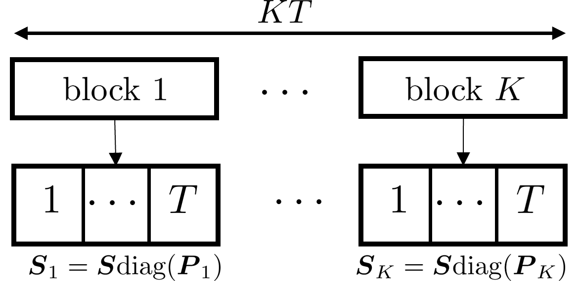
Figure 1: Transmission protocol.

Scattering matrix design

Starting from the fundamental signal model in (8), we propose to design the BD-RIS training matrix as a product of a fixed scattering matrix $\boldsymbol{S}_{0}$ and a block-dependent diagonal rotation, such that $\boldsymbol{S}_{k}^{(q)}=\boldsymbol{S}_{0}\text{diag}(\boldsymbol{\overline{p}}_{k}^{(q)})$ where $\boldsymbol{\overline{p}}_{k,q}$ is the vector containing the phase rotation angles associated with the $q$th group and $k$th block subject to $(\boldsymbol{S}_{k}^{(q)})^{\text{H}}\boldsymbol{S}_{k}^{(q)}=\boldsymbol{S}_{k}^{(q)}(\boldsymbol{S}_{k}^{(q)})^{\text{H}}=\boldsymbol{I}_{N_{q}}.$

III Semi-blind PARatuck rEceiver (PARE)

Assuming the noiseless case for notation convenience, the received signal can be expressed as

$$\boldsymbol{Y}_{k} =\left(\sum_{q=1}^{Q}\boldsymbol{H}^{(q)}\boldsymbol{S}_{0}^{(q)}\text{diag}(\boldsymbol{\overline{p}}_{k}^{(q)})\boldsymbol{G}^{(q)}\text{diag}(\boldsymbol{w}_{k})\boldsymbol{X}^{\text{T}}\right)$$ (9)

$$=\boldsymbol{H}\boldsymbol{S}\text{diag}(\boldsymbol{p}_{k})\boldsymbol{G}\text{diag}(\boldsymbol{w}_{k})\boldsymbol{X}^{\text{T}},$$

where $\boldsymbol{H}\doteq\left[\boldsymbol{H}_{1}\;\dots\;\boldsymbol{H}_{Q}\right]\in\boldsymbol{C}^{M_{R}\times N}$, $\boldsymbol{G}\doteq\left[\boldsymbol{G}_{1}^{\text{T}}\;\dots\;\boldsymbol{G}_{Q}^{\text{T}}\right]^{\text{T}}\in\boldsymbol{C}^{N\times M_{T}}$ are the Rx-RIS and TX-RIS channels, respectively, while $\boldsymbol{p}_{k}\doteq[\boldsymbol{p}^{(1)\text{T}}_{k},\ldots,\boldsymbol{p}^{(Q)\text{T}}_{k}]^{\text{T}}\in\mathbb{C}^{N\times 1}$, and $\boldsymbol{S}\doteq\text{bdiag}(\boldsymbol{S}_{0}^{(1)},\ldots\boldsymbol{S}_{0}^{(Q)})\in\mathbb{C}^{N\times N}$, with $\boldsymbol{S}_{0}^{(q)}\boldsymbol{S}_{0}^{(q)\text{H}}=\boldsymbol{I}_{N_{q}}$. Let us define $\boldsymbol{P}=[\boldsymbol{p}_{1},\ldots,\boldsymbol{p}_{K}]^{\text{T}}\in\mathbb{C}^{K\times N}$ and $\boldsymbol{W}\doteq[\boldsymbol{w}_{1},\ldots,\boldsymbol{w}_{K}]^{\text{T}}\in\mathbb{C}^{K\times M_{T}}$ as the BD-RIS phase rotation matrix and the transmitter side coding matrix, respectively. Additionally, let $\overline{\boldsymbol{H}}=\boldsymbol{H}\boldsymbol{S}\in\mathbb{C}^{M_{R}\times N}$ be the effective BS-RIS channel matrix. With these definitions, we can rewrite the noiseless received signal as the $k$-th block as

$$\boldsymbol{Y}_{k}=\overline{\boldsymbol{H}}D_{k}(\boldsymbol{P})\boldsymbol{G}D_{k}(\boldsymbol{W})\boldsymbol{X}^{\text{T}}\in\mathbb{C}^{M_{R}\times T},\,\,k=1,\ldots,K.$$ (10)

We can view the received signal matrices $\{\boldsymbol{Y}_{1},\ldots,\boldsymbol{Y}_{K}\}$ as frontal slices of a thrid-order tensor $\boldsymbol{\mathcal{Y}}\in\mathbb{C}^{M_{R}\times T\times K}$. In fact, the signal model (10) corresponds to a PARATUCK tensor model [23, 11]. To summarize, comparing equations (5) and (10), the following correspondence can be established

$$\left(\boldsymbol{A},\boldsymbol{B},\boldsymbol{\Omega},\boldsymbol{C}^{\boldsymbol{A}},\boldsymbol{C}^{\boldsymbol{B}}\right)\leftrightarrow(\boldsymbol{HS},\boldsymbol{X},\boldsymbol{G},\boldsymbol{P},\boldsymbol{W}).$$ (11)

To jointly estimate the involved channels and the transmitted data symbol matrices, we formulate the following optimization problem:

$$(\hat{\overline{\boldsymbol{H}}},\hat{\boldsymbol{G}},\hat{\boldsymbol{X})}=\underset{\overline{\boldsymbol{H}},\boldsymbol{G},\boldsymbol{X}}{\textrm{min}}\,\,\sum\limits_{k=1}^{K}\Big{\|}\boldsymbol{Y}_{k}-\overline{\boldsymbol{H}}D_{k}(\boldsymbol{S})\boldsymbol{G}D_{k}(\boldsymbol{W})\boldsymbol{X}^{\text{T}}\Big{\|}^{2}_{F}.$$ (12)

Since the problem is nonlinear with respect to the unknown matrices we exploit its multilinear structure and recast it as a set of three conditionally linear problems solved iteratively [12]. Specifically, one matrix is updated at each iteration by fixing the other two at the values obtained in previous steps.

III-A Estimation of the RIS-Rx channel $\overline{\boldsymbol{H}}$

Consider the received signal in (10). After $K$ blocks, we can collect all signals in the 1-mode unfolding as

$$[\boldsymbol{\mathcal{Y}}]_{(1)}\doteq\big{[}\boldsymbol{Y}_{1},\ldots,\boldsymbol{Y}_{K}\big{]}=\overline{\boldsymbol{H}}\boldsymbol{F}^{\text{T}}\,\,\in\mathbb{C}^{M_{R}\times TK},$$ (13)

where

$$\Big{[}\left(\boldsymbol{X}D_{1}(\boldsymbol{W})\boldsymbol{G}^{\text{T}}D_{1}(\boldsymbol{P})\right)^{\text{T}}\;\dots\;\left(\boldsymbol{X}D_{K}(\boldsymbol{W})\boldsymbol{G}^{\text{T}}D_{K}(\boldsymbol{P})\right)^{\text{T}}\Big{]}^{\text{T}}$$ (14)

To estimate $\overline{\boldsymbol{H}}$ we need to solve the following LS problem

$$\hat{\overline{\boldsymbol{H}}}=\underset{\overline{\boldsymbol{H}}}{\arg\min}\,\,\left\|[\boldsymbol{\mathcal{Y}}]_{(1)}-\overline{\boldsymbol{H}}\boldsymbol{F}^{\text{T}}\right\|_{F}^{2},$$ (15)

the solution of which is given by

$$\hat{\overline{\boldsymbol{H}}}=[\boldsymbol{\mathcal{Y}}]_{(1)}\left(\boldsymbol{F}^{\text{T}}\right)^{\dagger}.$$ (16)

From $\hat{\overline{\boldsymbol{H}}}$ the estimate of $\hat{\boldsymbol{H}}$ is given filtering the block diagonal phase shift $\boldsymbol{S}$ as $\hat{\boldsymbol{H}}=\hat{\overline{\boldsymbol{H}}}\boldsymbol{S}^{\text{H}}\;.$

III-B Symbol estimation

In a similar way, we get the $2$-mode unfolding as follows

$$[\boldsymbol{\mathcal{Y}}]_{(2)}\doteq\big{[}\boldsymbol{Y}_{1}^{\text{T}},\ldots,\boldsymbol{Y}_{K}^{\text{T}}\big{]}=\boldsymbol{X}\boldsymbol{E}^{\text{T}}\,\,\in\mathbb{C}^{T\times M_{R}K},$$ (17)

where

$$\Big{[}\left(\overline{\boldsymbol{H}}D_{1}(\boldsymbol{S})\boldsymbol{G}D_{1}(\boldsymbol{W})\right)^{\text{T}}\;\dots\;\left(\overline{\boldsymbol{H}}D_{K}(\boldsymbol{S})\boldsymbol{G}D_{K}(\boldsymbol{W})\right)^{\text{T}}\Big{]}^{\text{T}}$$ (18)

To estimate $\boldsymbol{X}$, we solve the following LS problem

$$\hat{\boldsymbol{X}}=\underset{\boldsymbol{X}}{\arg\min}\,\,\left\|[\boldsymbol{\mathcal{Y}}]_{(2)}-\boldsymbol{X}\boldsymbol{E}^{\text{T}}\right\|_{F}^{2},$$ (19)

the solution of which is given by:

$$\hat{\boldsymbol{X}}=[\boldsymbol{\mathcal{Y}}]_{(2)}\left(\boldsymbol{E}^{\text{T}}\right)^{\dagger}.$$ (20)

III-C Estimation of the Tx-RIS channel $\boldsymbol{G}$

To estimate the Tx-RIS channel matrix $\boldsymbol{G}$, let us apply the $\textrm{vec}(.)$ and the properties (1) and (3), such that the vectorized form of the received signal (10), is given as

$$\textrm{vec}\left(\boldsymbol{Y}_{k}\right) =(\boldsymbol{X}\otimes\overline{\boldsymbol{H}})\textrm{vec}\left(D_{k}(\boldsymbol{P})\boldsymbol{G}D_{k}(\boldsymbol{W})\right)$$ (21)

$$=(\boldsymbol{X}\otimes\overline{\boldsymbol{H}})\left(D_{k}(\boldsymbol{W})\otimes D_{k}(\boldsymbol{P})\right)\textrm{vec}(\textbf{G})\,,$$

Note that $\left(D_{k}(\boldsymbol{W})\otimes D_{k}(\boldsymbol{P})\right)$ is actually $\textrm{diag}\left(\boldsymbol{W}_{k\cdot}^{\text{T}}\otimes\boldsymbol{P}_{k\cdot}^{\text{T}}\right)$. Then, applying the property (2) to (21) yields

$$\textrm{vec}\left(\boldsymbol{Y}_{k}\right)=(\boldsymbol{X}\otimes\overline{\boldsymbol{H}})\textrm{diag}(\textrm{vec}(\boldsymbol{G}))\big{(}\boldsymbol{W}_{k\cdot}^{\text{T}}\otimes\boldsymbol{P}_{k\cdot}^{\text{T}}\big{)},$$ (22)

By collecting the vectorized version of the $K$ received signal blocks, we can build the 3-mode unfolding of the received signal tensor, which can be expressed as

₍₃₎ $$\doteq\big{[}\textrm{vec}\left(\boldsymbol{Y}_{1}\right),\ldots,\textrm{vec}\left(\boldsymbol{Y}_{K}\right)\big{]}$$ (23)

$$=(\boldsymbol{X}\otimes\overline{\boldsymbol{H}})\textrm{diag}(\textrm{vec}(\boldsymbol{G}))\boldsymbol{\Psi}\,,\,\in\,\mathbb{C}^{TM\times K}$$

where

$$\boldsymbol{\Psi} \doteq\left[\boldsymbol{W}_{1\cdot}^{\text{T}}\otimes\boldsymbol{P}_{1\cdot}^{\text{T}},\ldots,\boldsymbol{W}_{K\cdot}^{\text{T}}\otimes\boldsymbol{P}_{K\cdot}^{\text{T}}\right]$$ (24)

$$=\boldsymbol{W}^{\text{T}}\diamond\boldsymbol{P}^{\text{T}}\in\mathbb{C}^{M_{T}N\times K}.$$

Then, vectorizing (23) yields

$$\textrm{vec}\left([\boldsymbol{\mathcal{Y}}]_{(3)}\right) =\big{[}\boldsymbol{\Psi}^{\text{T}}\diamond(\boldsymbol{X}\otimes\overline{\boldsymbol{H}})\big{]}\textrm{vec}(\boldsymbol{G})+\textrm{vec}\left(\boldsymbol{B}_{3}\right).$$ (25)

Finally, an estimate of $\boldsymbol{G}$ in the LS sense can be obtained by solving the following problem

$$\hat{\boldsymbol{G}}=\underset{\boldsymbol{G}}{\arg\min}\,\,\left\|\textrm{vec}\left([\boldsymbol{\mathcal{Y}}]_{(3)}\right)-\big{[}\boldsymbol{\Psi}^{\text{T}}\diamond(\boldsymbol{X}\otimes\overline{\boldsymbol{H}})\big{]}^{\dagger}\textrm{vec}(\boldsymbol{G})\right\|_{F}^{2},$$ (26)

the solution of which is given by

$$\hat{\boldsymbol{G}}=\textrm{unvec}_{N\times L}\Big{(}\left[\boldsymbol{\Psi}^{\text{T}}\diamond(\boldsymbol{X}\otimes\overline{\boldsymbol{H}})\right]^{\dagger}\textrm{vec}([\boldsymbol{\mathcal{Y}}]_{(3)})\Big{)}.$$ (27)

The proposed semi-blind receiver utilizes equations (16), (20), and (27) to estimate channel matrices $\boldsymbol{H}$ and $\boldsymbol{X}$, as well as the symbol $\boldsymbol{G}$ through a trilinear alternating least squares based estimation scheme, which is known as the trilinear alternating least squares (TALS) receiver summarized in the algorithm in Algorithm 1. The stopping criterion used in this work is based on the normalized squared error measure, which is computed at the end of each iteration. The error measure is denoted as $\epsilon_{(i)}$ and is given by the following equation: $\epsilon_{(i)}=\sum\limits_{k=1}^{K}\|\boldsymbol{Y}_{k}-\hat{\boldsymbol{Y}}_{k_{(i)}}\|_{F}^{2}/\|\boldsymbol{Y}_{k}\|_{F}^{2}$. Here, $\hat{\boldsymbol{Y}}_{k_{(i)}}=\hat{\boldsymbol{H}}_{(i)}D_{k}(\boldsymbol{S})\hat{\boldsymbol{G}}_{(i)}D_{k}(\boldsymbol{W})\hat{\boldsymbol{X}}^{\textrm{T}}_{(i)}$. Convergence is declared when the difference between the reconstruction errors of two successive iterations falls below a threshold, which is represented by $|\epsilon_{(i)}-\epsilon_{(i-1)}|\leq\delta$. In this work, we have assumed $\delta=10^{-5}$.

Procedure

input : $i=0$; Initialize $\hat{\boldsymbol{G}}_{(i=0)}$ and $\hat{\boldsymbol{X}}_{(i=0)}$

output : $\hat{\boldsymbol{H}}$, $\hat{\boldsymbol{G}}$ and $\hat{\boldsymbol{X}}$

begin

       $i=1;$

       while $\|e(i)-e(i-1)\|\geq\delta$ do

1.        

   Using $\hat{\boldsymbol{G}}_{(i-1)}$ and $\hat{\boldsymbol{X}}_{(i-1)},$ compute

             $\hat{\boldsymbol{F}}_{(i-1)}$ from (14) and find

             a least squares estimate of $\boldsymbol{H}$:

$\hat{\overline{\boldsymbol{H}}}_{(i)}=\boldsymbol{Y}_{1}\left(\hat{\boldsymbol{F}}^{\textrm{T}}_{(i-1)}\right)^{\dagger}\rightarrow$ $\hat{\boldsymbol{H}}=\hat{\overline{\boldsymbol{H}}}\boldsymbol{S}^{\text{H}}$

       

Using $\hat{\boldsymbol{H}}_{(i)}$ and $\hat{\boldsymbol{X}}_{(i-1)}$, find

             a least squares estimate of $\boldsymbol{G}$:

$\textrm{vec}(\hat{\boldsymbol{G}}_{(i)})=\left[\boldsymbol{\Psi}^{\textrm{T}}\diamond(\boldsymbol{X}_{(i-1)}\otimes\boldsymbol{H}_{(i)})\right]^{\dagger}\textrm{vec}(\boldsymbol{Y}_{3})$

       

Using $\hat{\boldsymbol{G}}_{(i)}$ and $\hat{\boldsymbol{H}}_{(i)},$ compute

             $\hat{\boldsymbol{E}}_{(i)}$ from (18) and find

             a least squares estimate of $\boldsymbol{X}$:

$\hat{\boldsymbol{X}}_{(i)}=\boldsymbol{Y}_{2}\left(\hat{\boldsymbol{E}}^{\textrm{T}}_{(i)}\right)^{\dagger}$

$i\leftarrow i+1$ 5:         Repeat steps $1$ to $4$ until convergence. end

      end

Algorithm 1 TALS

III-D Identifiability and complexity

The joint recovery of $\boldsymbol{H}$, $\boldsymbol{X}$, and $\boldsymbol{G}$ requires that the three LS problems in (15), (19) and (26) have unique solutions, respectively. More specifically, the uniqueness of $\boldsymbol{H}$ requires that $\boldsymbol{F}$ defined in (14) have a full column rank, which implies $TK\geq N$, while the uniqueness of $\boldsymbol{G}$ requires that $\left[\boldsymbol{\Psi}^{\textrm{T}}\diamond(\boldsymbol{X}\otimes\boldsymbol{H})\right]$ have a full column rank, which implies $TKM_{R}\geq M_{T}N$. Likewise, the uniqueness of $\boldsymbol{X}$ requires that $\boldsymbol{E}$ defined in (18) be of full column-rank, which implies $M_{R}K\geq M_{T}$. In summary, the following conditions must hold for the joint uniqueness of $\boldsymbol{H}$, $\boldsymbol{G}$, and $\boldsymbol{X}$: $TK\geq N,\quad TKM_{R}\geq M_{T}N,\quad M_{R}K\geq M_{T}.$ These conditions establish useful trade-offs involving the time diversities (parameters $K$ and $T$) and spatial diversities (parameters $N$, $M_{R}$, $M_{T}$) for the joint recovery of the channel and symbol matrices.The complexity of the algorithm 1 is dominated by the pseudo-inverse calculation in step $2$. Considering that the computational complexity of the pseudo-inverse is equivalent to that of the singular value decomposition (SVD), the complexity of our proposed solution is $\mathcal{O}(TKM_{R}(M_{T}N)^{2})$.

IV Performance evaluation

We evaluate the performance of the proposed semi-blind receivers. The channel estimation (CE) accuracy is evaluated in terms of the normalized mean square error (NMSE) given by $\textrm{NMSE}(\hat{\boldsymbol{\Pi}})=\frac{1}{R}\sum_{r=1}^{R}\dfrac{\|\boldsymbol{\Pi}^{(r)}-\hat{\boldsymbol{\Pi}}^{(r)}\|_{F}^{2}}{\|\boldsymbol{\Pi}^{(r)}\|_{F}^{2}}$, where $\boldsymbol{\Pi}=\boldsymbol{H},\boldsymbol{G}$ and $\hat{\boldsymbol{\Pi}}^{(r)}$ denotes the estimation of the channels at the $r$th run, and $R$ denotes the number of Monte-Carlo runs. We also evaluate both the symbol error rate (SER) performance and complexity in terms of the number of iterations as a function of the signal-to-noise ratio (SNR). Regarding the channel model, we consider the Rayleigh fading case (i.e. the entries of channel matrices are independent and identically distributed zero-mean circularly-symmetric complex Gaussian random variables. All results represent an average of at least $R=3000$ Monte Carlo runs. Each run corresponds to an independent realization of the channel matrices, transmitted symbols, and the noise term.

We assume $M_{R}=5$, $M_{T}=2$, $K=20$, $T=10$, and $N=16$ with $Q={4,8}$. The scattering matrix for the group $q$, $\boldsymbol{S}_{q}$, as well as the rotation and coding matrices $\boldsymbol{P}$ and $\boldsymbol{W}$, respectively, can be a proper DFT. Figure 2 depicts the channel estimation performance in terms of normalized mean squared error (NMSE). The accuracy of channel estimation $\boldsymbol{G}$ is better than that of $\boldsymbol{H}$, as the former requires a spatial filter step to obtain this channel estimation. Considering the composed channel $\boldsymbol{H}_{c}=\boldsymbol{G}^{\text{T}}\otimes\boldsymbol{H}$, we present a comparison of our proposed method with existing approaches in the literature, specifically the least squares (LS) method [3] and the block Tucker Khatri-Rao factorization (BTKF) method [9], as shown in Figure 3. We assume the parameter set $Q=2$, $N=16$, $M_{R}=M_{T}=4$, and $KT=M_{T}N_{q}^{2}Q$ to ensure a fair comparison with the reference methods. First, we can see that the proposed method outperforms the LS method. This improvement is due to the noise rejection gain achieved by our iterative approach, which enables decoupled channel estimation. We can also note that the proposed PARE receiver exhibit has a performance gap in comparison to the reference BTKF channel estimation method. However, it is important to note that both LS and BTKF are pilot-assisted methods, while PARE is a semi-blind receiver that uses actual data symbols to estimate the individual channels. This means that, compared to BTKF, the proposed receiver offers a higher spectral efficiency by allowing joint symbol decoding and channel estimation. More specifically, the PARE receiver enables decoding of $M_{T}$ useful data streams during the channel estimation process, therefore exhibiting a smaller data decoding delay compared to competing pilot-assisted methods for BD-RIS. Additionally, PARE can operate under more flexible system parameter settings than its competitors. Although we have selected $KT=M_{T}N_{q}^{2}Q$ $(K=64\;\text{and}\;T=8)$ to meet the constraints of the competing methods, PARE can operate under different choices of $K$ and $T$ allowing to trade performance and spectral efficiency.

Figure 2: NMSE vs. SNR

Figure 3: NMSE of equivalent channel vs. SNR

Figure 4 depicts the SER performance for two different numbers of BD-RIS groups. The performance of the zero-forcing (ZF) receiver under perfect channel knowledge is also shown as a reference. Note that increasing the number of groups produces improved SER and implies a reduced complexity in the number of iterations, as illustrated in the results of Figure 5. From this figure, we can also see that the convergence of Algorithm 1 is usually achieved within 20 iterations in the moderate SNR range for the considered parameter settings.

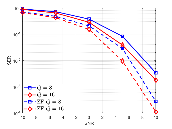
Figure 4: SER vs SNR

Figure 5: Average runtime vs. SNR

V Conclusion

This paper addressed semi-blind channel estimation for BD-RIS. The proposed PARE receiver provides joint channel and symbol estimation based on an alternating estimation scheme derived from a PARATUCK tensor modeling of the received signals. Our proposed receiver enjoys more flexible system parameter choices than traditional LS-based estimation while allowing a data-aided channel estimation without a prior training stage. A perspective of this work includes alternative BD-RIS design structures and extensions to multi-user scenarios.

References

- [1] B. Zheng, C. You, W. Mei, and R. Zhang, “A survey on channel estimation and practical passive beamforming design for intelligent reflecting surface aided wireless communications,” IEEE Commun. Surveys Tuts., vol. 24, no. 2, pp. 1035–1071, Feb. 2022.
- [2] H. Li, S. Shen, and B. Clerckx, “Beyond diagonal reconfigurable intelligent surfaces: From transmitting and reflecting modes to single-, group-, and fully-connected architectures,” IEEE Trans. Wireless Commun., vol. 22, no. 4, pp. 2311–2324, 2023.
- [3] H. Li, S. Shen, Y. Zhang, and B. Clerckx, “Channel estimation and beamforming for beyond diagonal reconfigurable intelligent surfaces,” IEEE Transactions on Signal Processing, vol. 72, pp. 3318–3332, 2024.
- [4] Q. Li, M. El-Hajjar, I. Hemadeh, A. Shojaeifard, A. A. M. Mourad, B. Clerckx, and L. Hanzo, “Reconfigurable intelligent surfaces relying on non-diagonal phase shift matrices,” IEEE Trans. Vehicular Tech., vol. 71, no. 6, pp. 6367–6383, 2022.
- [5] S. Shen, B. Clerckx, and R. Murch, “Modeling and architecture design of reconfigurable intelligent surfaces using scattering parameter network analysis,” IEEE Transactions on Wireless Communications, vol. 21, no. 2, pp. 1229–1243, 2022.
- [6] M. Nerini, S. Shen, H. Li, M. Di Renzo, and B. Clerckx, “A universal framework for multiport network analysis of reconfigurable intelligent surfaces,” IEEE Transactions on Wireless Communications, vol. 23, no. 10, pp. 14 575–14 590, 2024.
- [7] M. Nerini, S. Shen, and B. Clerckx, “Closed-form global optimization of beyond diagonal reconfigurable intelligent surfaces,” IEEE Trans. Wireless Commun., vol. 23, no. 2, pp. 1037–1051, 2024.
- [8] M. Soleymani, I. Santamaria, E. Jorswieck, and B. Clerckx, “Optimization of rate-splitting multiple access in beyond diagonal RIS-assisted urllc systems,” IEEE Trans. Wireless Commun., pp. 1–1, 2023.
- [9] A. L. F. de Almeida, B. Sokal, H. Li, and B. Clerckx, “Channel estimation for beyond diagonal ris via tensor decomposition,” 2024. [Online]. Available: https://arxiv.org/abs/2407.20402
- [10] L. R. Ximenes, G. Favier, A. L. F. de Almeida, and Y. C. B. Silva, “PARAFAC-PARATUCK semi-blind receivers for two-hop cooperative MIMO relay systems,” IEEE Trans. Sig. Proces., vol. 62, no. 14, pp. 3604–3615, 2014.
- [11] G. T. de Araújo, A. L. F. de Almeida, R. Boyer, and G. Fodor, “Semi-blind joint channel and symbol estimation for IRS-assisted MIMO systems,” IEEE Trans. Sig. Proces., vol. 71, pp. 1184–1199, 2023.
- [12] P. Comon, X. Luciani, and A. L. F. de Almeida, “Tensor decompositions, alternating least squares and other tales,” Journal of Chemometrics, vol. 23, no. 7-8, pp. 393–405, 2009. [Online]. Available: https://analyticalsciencejournals.onlinelibrary.wiley.com/doi/abs/10.1002/cem.1236
- [13] A. L. F. de Almeida, G. Favier, and J. C. M. Mota, “PARAFAC-based unified tensor modeling for wireless communication systems with application to blind multiuser equalization,” Signal Processing, vol. 87, no. 2, pp. 337–351, 2007, tensor Signal Processing.
- [14] A. L. F. de Almeida, G. Favier, and J. C. M. Mota, “A constrained factor decomposition with application to mimo antenna systems,” IEEE Transactions on Signal Processing, vol. 56, no. 6, pp. 2429–2442, 2008.
- [15] G. Favier and A. L. F. de Almeida, “Tensor space-time-frequency coding with semi-blind receivers for MIMO wireless communication systems,” IEEE Trans. Signal Process., vol. 62, no. 22, pp. 5987–6002, 11 2014.
- [16] L. R. Ximenes, G. Favier, and A. L. F. de Almeida, “Semi-blind receivers for non-regenerative cooperative mimo communications based on nested parafac modeling,” IEEE Transactions on Signal Processing, vol. 63, no. 18, pp. 4985–4998, 2015.
- [17] H. Chen, F. Ahmad, S. Vorobyov, and F. Porikli, “Tensor decompositions in wireless communications and mimo radar,” IEEE Journal of Selected Topics in Signal Processing, vol. 15, no. 3, pp. 438–453, 2021.
- [18] G. T. de Araújo and A. L. F. de Almeida, “PARAFAC-based channel estimation for intelligent reflective surface assisted mimo system,” in 2020 IEEE 11th Sensor Array and Multichannel Signal Processing Workshop (SAM), 2020, pp. 1–5.
- [19] G. T. de Araújo, A. L. F. de Almeida, and R. Boyer, “Channel estimation for intelligent reflecting surface assisted MIMO systems: A tensor modeling approach,” IEEE J. Sel. Topics Signal Process., vol. 15, no. 3, pp. 789–802, Apr 2021.
- [20] R. A. Harshman and M. E. Lundy, “Uniqueness proof for a family of models sharing features of tucker′s three-mode factor analysis and PARAFAC/CANDECOMP,” in Psychometrika, vol. 61, Mar. 1996, pp. 133–154.
- [21] L. R. Tucker, “Some mathematical notes on three-mode factor analysis,” Psychometrika, vol. 31, no. 3, p. 279–311, Sep. 1966.
- [22] H. Li, Y. Zhang, and B. Clerckx, “Channel estimation for beyond diagonal reconfigurable intelligent surfaces with group-connected architectures,” in (CAMSAP), 2023, pp. 21–25.
- [23] X. Han, A. L. F. de Almeida, and Z. Yang, “Channel estimation for MIMO multi-relay systems using a tensor approach,” EURASIP J. Adv. Signal Process, 2014.