Application of the Direct Interaction Approximation to generalized stochastic models in the turbulence problem

Abstract

The purpose of this paper is to consider the application of the direct interaction approximation (DIA) developed by Kraichnan [1], [2] to generalized stochastic models in the turbulence problem. Previous developments (Kraichnan [1], [2], Shivamoggi et al. [7], Shivamoggi and Tuovila [8]) were based on the Boltzmann-Gibbs prescription for the underlying entropy measure, which exhibits the extensivity property and is suited for ergodic systems. Here, we consider the introduction of an influence bias discriminating rare and frequent events explicitly, as behooves non-ergodic systems. More specifically, we consider the application of the DIA to a linear damped stochastic oscillator system using a Tsallis type [12] autocorrelation model with an underlying non-extensive entropy measure, and describe the resulting stochastic process. We also deduce some apparently novel mathematical properties of the stochastic models associated with the present investigation – the gamma distribution (Andrews et al. [13], [14]) and the Tsallis non-extensive entropy [12].

1 Introduction

The direct-interaction approximation (DIA) advanced by Kraichnan [1], [2] is currently the only fully self-consistent analytical theory of turbulence in fluids. The formal application of the DIA to a statistical problem is justified only when the nonlinear effects are weak. Since this is not the case in the turbulence problem, there is a need to rationalize the DIA prior to application via a model equation which can be solved exactly. Kraichnan [2] applied the DIA to the model equation and modified it by a process, where the non-linear terms are unrestricted, into another equation for which the DIA gives the exact statistical average.

Several mathematical issues associated with the application of the DIA to Kraichnan’s [1] stochastic model equation were explored by Shivamoggi, et al. [7] and Shivamoggi and Tuovila [8]. Kraichnan [1] considered a stochastic model with fluctuations having short-range correlations. Shivamoggi, et al. [7] considered instead fluctuations following an Uhlenbeck-Ornstein process [9] with wide-ranging correlations. The stochastic models of Kraichnan [1] and Shivamoggi et al. [7] are based on a Markovian process. Shivamoggi and Tuovila [8], on the other hand, considered a stochastic model based on an ultra non-Markovian process. All these developments were based on the Boltzmann-Gibbs prescription for the underlying entropy measure, which complies with the extensivity property and is suited for ergodic systems. However, non-ergodic, non-Markovian systems need the introduction of an influence bias discriminating rare and frequent events explicitly. In order to address this issue, Tsallis [12] gave a prescription to generalize the concept of entropy embodying a non-extensivity property to cover such systems.

In this paper, we consider the application of the DIA to a linear damped stochastic oscillator system using a Tsallis type [12] autocorrelation model with an underlying non-extensive entropy measure, and describe the resulting stochastic process. We also deduce some apparently novel mathematical properties of the stochastic models associated with the present investigation – the gamma distribution (Andrews et al. [13], [14]) and the Tsallis non-extensive entropy [12].

2 Tsallis entropy model

The Boltzmann-Gibbs entropy of a system with $W$ microstates, each of which has probability $p_{i}$, is given by the formula

$$S_{BG}=-k_{B}\sum_{i=1}^{W}p_{i}\ln p_{i}$$ (1)

with the normalization condition

$$\sum_{i=1}^{W}p_{i}=1.$$ (2)

Here, $k_{B}$ is the Boltzmann constant, which we will put equal to unity for convenience. In the case of equiprobability, $p_{i}=1/W,\forall i$, eq(1) then reduces to the Boltzmann ansatz,

$$S_{BG}=\ln W.$$ (3)

The Boltzmann-Gibbs entropy is nonnegative, concave, experimentally robust, and extensive. The latter property implies that for two independent statistical systems $A$ and $B$,

$$S_{BG}(A+B)=S_{BG}(A)+S_{BG}(B).$$ (4)

Just as $S_{BG}$ is postulated, so is its generalization. Tsallis [12] proposed the following model for entropy (see Appendix A for a mathematical motivation of this),

$$S_{q}=\frac{1-\sum_{i=1}^{W}p_{i}^{q}}{q-1}$$ (5)

where $q$ is the parameter characterizing the non-extensivity of the entropy. (5) yields, in the Boltzmann-Gibbs (extensive entropy, $q\to 1$) limit,

$$S_{1}=\lim_{q\to 1}S_{q}=-\sum_{i=1}^{W}p_{i}\ln p_{i}.$$ (1)

On maximizing $S_{q}$, subject to the constraints,

• generalized normalization:

  $$\sum_{i}P_{i}(q)=1$$ (6)

• generalized energy conservation:

  $$\sum_{i}P_{i}(q)E_{i}=\text{const}\equiv U_{q}$$ (7)

where $P_{i}(q)$ are the escort probabilities,

$$P_{i}(q)\equiv\frac{p_{i}^{q}}{\sum_{i}p_{i}^{q}}$$ (8)

and $E_{i}$ is the energy of the $i$th state, we obtain

$$\overline{p_{i}}=\frac{1}{Z_{q}}\biggl{[}1-(1-q)\beta E_{i}\biggr{]}^{\frac{1}{1-q}}.$$ (9)

Here, $\beta$ is the Lagrange multiplier, and $Z_{q}$ is the partition function ensuring normalization, such that

$$\sum_{i}\overline{p_{i}}=1.$$ (10)

In the Boltzmann-Gibbs limit, (9) gives the usual result,

$$\lim_{q\to 1}\overline{p_{i}}\sim e^{-\beta E_{i}},$$ (11)

so (9) may be viewed as a one-parameter generalization of the Boltzmann-Gibbs formula (11). On the other hand, for $q<1$, (9) implies the compatibility condition,

$$1-(1-q)\beta E_{i}<0\,:\,\overline{p_{i}}=0.$$ (12)

3 Tsallis autocorrelation model via compound statistics of the Uhlenbeck-Ornstein model for a random process

Consider a random process described by a real, centered, stationary Gaussian random function $b(t)$, which follows the Uhlenbeck-Ornstein model [9]. We then follow the ansatz of Wilk and Wlodarcyzk [15] and Beck [16] for the Boltzmann distribution and account for a slowly varying environment of the latter model by stipulating the governing parameter $\lambda$ (the inverse autocorrelation time) thereof to follow a gamma distribution, hence compounding the statistics underlying the Uhlenbeck-Ornstein model.

Consider the Uhlenbeck-Ornstein model for the conditional autocorrelation function of this stationary random process,

$$r(t^{\prime},t^{\prime\prime},\lambda)\equiv\langle b(t^{\prime})b(t^{\prime\prime})\rangle=\sigma^{2}e^{-\lambda(t^{\prime}-t^{\prime\prime})}.$$ (13)

Suppose the inverse autocorrelation time $\lambda$ is also a random variable distributed according to a gamma distribution,

$$f(\lambda;c)=\frac{1}{a\Gamma(c)}\bigg{(}\frac{\lambda}{a}\bigg{)}^{c-1}e^{-\lambda/a},\,a>0,\,c>0.$$ (14)

(14) leads to the following expression for the mean $\lambda_{0}$ and the variance $\sigma^{2}$ of the random variable $\lambda$,

$$\lambda_{0}\equiv\langle\lambda\rangle=\int_{0}^{\infty}\lambda f(\lambda;c)d\lambda=ac$$ (15a)

$$\sigma^{2}\equiv\langle\lambda^{2}\rangle-\langle\lambda\rangle^{2}=a^{2}c$$ (15b)

from which, we obtain for the parameters $$a c$$ and ,

$$a=\frac{\sigma^{2}}{\lambda_{0}},\,\,c=\frac{\lambda_{0}^{2}}{\sigma^{2}}.$$ (15c)

The marginal distribution is then given by averaging the conditional distribution $r(t^{\prime},t^{\prime\prime},\lambda)$ over $\lambda$,

$$\begin{split}R(t^{\prime},t^{\prime\prime})&=R(\tau)\equiv\int_{0}^{\infty}r(\tau,\lambda)f(\lambda;c)d\lambda\\ &=\frac{{\sigma}^{2}}{\Gamma(c)}\int_{0}^{\infty}\biggl{(}\frac{\lambda}{a}\biggr{)}^{c-1}e^{-(1+a\tau)(\lambda/a)}d\left(\frac{\lambda}{a}\right)\\ &=\frac{{\sigma}^{2}}{(1+a\tau)^{c}},\,\,\tau\equiv t^{\prime}-t^{\prime\prime}.\end{split}$$ (16)

Putting (Beck [16]),

$$c\equiv\frac{1}{q-1},$$ (17)

(16) leads to the Tsallis [12] type autocorrelation function,

$$R_{q}(\tau)={\sigma}^{2}[1-(1-q)\lambda_{0}\tau]^{\frac{1}{1-q}}$$ (18)

On writing (18) in terms of the q-exponential,

$$R_{q}(\tau)\equiv\sigma^{2}e_{q}^{-\lambda_{0}\tau},$$ (19a)

and noting that

$$\lim_{q\to 1}e_{q}^{-\lambda_{0}\tau}=e^{-\lambda_{0}\tau},$$ (19b)

$$q$$ is observed to play the role of the non-extensivity parameter.

Furthermore, we have from (15) and (17),

$$\sigma^{2}=(q-1)\lambda_{0}^{2}$$ (20)

which implies,

$$q\equiv\frac{\langle\lambda^{2}\rangle}{\lambda_{0}^{2}}>1.$$ (21)

On the other hand, we have, in the zero-dispersion limit (see Appendix B),

$$\lim_{c\to\infty}f(\lambda;c)=\delta(\lambda-\lambda_{0}).$$ (22)

We therefore obtain the Uhlenbeck-Ornstein autocorrelation function in the extensive entropy limit, ($q\to 1$),

$$R_{1}(\tau)=\lim_{q\to 1}R_{q}(\tau)\equiv\lim_{q\to 1}\sigma^{2}e_{q}^{\lambda_{0}\tau}={\sigma}^{2}e^{-\lambda_{0}\tau}$$ (23)

with the inverse autocorrelation time given by $\lambda_{0}$.

Some mathematical properties of the marginal distribution (18) are discussed in Appendix C and Appendix D.

4 Linear damped stochastic oscillator

Consider the linear damped stochastic oscillator described by the IVP (Zwanzig [17]),

$$[\frac{d}{dt}+ib(t)]\hat{G}(t)+\int_{0}^{t}\Gamma(t-t^{\prime})\hat{G}(t^{\prime})dt^{\prime}=\delta(t),\,\hat{G}(0)=1$$ (24a)

where $$\Gamma(t)$$ is a history-dependent damping coefficient,

$$\Gamma(t)=\nu e^{-\mu t},\,\,\nu\text{ and }\mu>0.$$ (24b)

In the limit $\mu\to\infty$, with $\displaystyle\lim_{\mu\to\infty}\frac{\nu}{\mu}=$ const, the damping process displays zero memory and becomes Markovian, explored first by Kraichnan [1] and then by Shivamoggi, et al. [7]. In this case, the IVP (24) leads to

$$[\frac{d}{dt}+\nu+ib(t)]\hat{G}(t)=\delta(t),\,\hat{G}(0)=1.$$ (25)

On the other hand, in the limit $\mu\to 0$, this process displays infinite memory and becomes ultra non-Markovian. The IVP (24) then leads to:

$$[\frac{d}{dt}+ib(t)]\hat{G}(t)+\nu\int_{0}^{t}\hat{G}(t^{\prime})dt^{\prime}=\delta(t),\,\hat{G}(0)=1$$ (26)

explored previously by Shivamoggi and Tuovila [8].

In both cases, $b(t)$ is a real, centered, stationary Gaussian random function of $t$ described by the Tsallis type [12] generalization of the Uhlenbeck-Ornstein model [9],

$$\langle b(t)b(t^{\prime})\rangle=\sigma^{2}e_{q}^{-\lambda(t-t^{\prime})}\equiv\sigma^{2}[1-\lambda\ell(t-t^{\prime})]^{\frac{1}{\ell}},\quad\ell\equiv 1-q.$$ (27)

Figure 1 shows the schematic of the theoretical considerations that follow below.

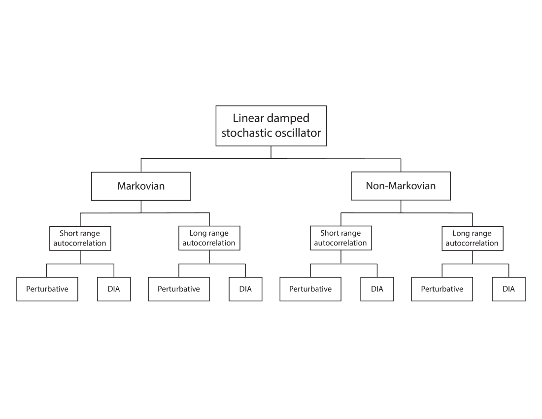
Figure 1: The schematic of the present discussion of the linear damped stochastic oscillator.

5 The Markovian Model

5.1 The long-range autocorrelation case

We consider first the case where the inverse autocorrelation time $\lambda$ is small.

5.1.1 Perturbative procedure

Applying Keller’s perturbation procedure [18], the IVP (25) becomes

$$\bigg{(}\frac{d}{dt}+\nu\bigg{)}G(t)+\int_{0}^{t}\langle b(t)b(t^{\prime})\rangle e^{-\nu(t-t^{\prime})}G(t^{\prime})dt^{\prime}=\delta(t),\qquad G(0)=1.$$ (28)

Putting

$$G(t)=e^{-\nu t}J(t)$$ (29)

and using the Tsallis type [12] autocorrelation model (27), the IVP (28) becomes

$$\frac{dJ}{dt}+\sigma^{2}\int_{0}^{t}[1-\lambda\ell(t-t^{\prime})]^{\frac{1}{\ell}}J(t^{\prime})dt^{\prime}=\delta(t),\enspace J(0)=1.$$ (30)

For small $\lambda$, using the Taylor series approximation (C.5), we obtain

$$\frac{dJ}{dt}+\sigma^{2}\int_{0}^{t}[1-\lambda(t-t^{\prime})]J(t^{\prime})dt^{\prime}=\delta(t),\,J(0)=1.$$ (31)

Applying the Laplace transform, the IVP (31) leads to

$$p\mathscr{J}(p)+\sigma^{2}\left[\frac{1}{p}\left(1-\frac{\lambda}{p}\right)\right]\mathscr{J}(p)=1.$$ (32)

Using the Padé approximation, eq(32) yields the functional equation

$$p\mathscr{J}(p)+\sigma^{2}\frac{\mathscr{J}(p)}{p+\lambda}=1,$$ (33)

which agrees with the results obtain by using the Uhlenbeck-Ornstein [9] model, given in [7].

5.1.2 DIA Procedure

Application of the DIA procedure to the IVP (25) involves replacing the perturbative expression for the deterministic Green’s function $e^{-\nu(t-t^{\prime})}$ in the IVP (28) by the exact expression $G(t-t^{\prime})$, yielding

$$\bigg{(}\frac{d}{dt}+\nu\bigg{)}G(t)+\int_{0}^{t}\langle b(t)b(t^{\prime})G(t-t^{\prime})\rangle G(t^{\prime})dt^{\prime}=\delta(t),\,G(0)=1.$$ (34)

Using the weak statistical-dependence hypothesis (Kraichnan [19], [20]), we may write

$$\langle b(t)b(t^{\prime})G(t-t^{\prime})\rangle=\langle b(t)b(t^{\prime})\rangle\langle G(t-t^{\prime})\rangle$$ (35)

and using (27) and (29), the IVP (34) becomes

$$\frac{dJ}{dt}+\sigma^{2}\int_{0}^{t}[1-\lambda\ell(t-t^{\prime})]^{\frac{1}{\ell}}J(t-t^{\prime})J(t^{\prime})dt^{\prime}=\delta(t),\enspace J(0)=1.$$ (36)

For small $\lambda$, using the Taylor series approximation (C.5) again, we obtain

$$\frac{dJ}{dt}+\sigma^{2}\int_{0}^{t}[1-\lambda(t-t^{\prime})]J(t-t^{\prime})J(t^{\prime})dt^{\prime}=\delta(t),\,J(0)=1.$$ (37)

Applying the Laplace transform, the IVP (37) leads to

$$p\mathscr{J}(p)+\sigma^{2}\left[\mathscr{J}(p)+\lambda\mathscr{J}^{\prime}(p)\right]\mathscr{J}(p)=1.$$ (38)

Noting that we may write, for small $\lambda$,

$$\mathscr{J}(p)+\lambda\mathscr{J}^{\prime}(p)\approx\mathscr{J}(p+\lambda)$$ (39)

eq(38) leads to the functional equation,

$$p\mathscr{J}(p)+\sigma^{2}\mathscr{J}(p+\lambda)\mathscr{J}(p)=1,$$ (40)

which agrees again with the results of [7] for the Markovian case.

5.2 The short-range autocorrelation case

In section 5.1, we considered the case for which the inverse autocorrelation time $\lambda$ is small. For large values of $\lambda$ (the white-noise limit), the Taylor series approximation (C.5) is no longer valid. Instead, we use, for small $\ell$, the delta function approximation established in Theorem 1 in Appendix C.

5.2.1 Perturbative procedure

Applying Keller’s perturbation procedure [18] and using the Tsallis type [12] autocorrelation model (27), the IVP (25) becomes

$$\frac{dJ}{dt}+\sigma^{2}\int_{0}^{t}[1-\lambda\ell(t-t^{\prime})]^{\frac{1}{\ell}}J(t^{\prime})dt^{\prime}=\delta(t),\enspace J(0)=1.$$ (30)

For large $\lambda$, using (C.6), the IVP (30) becomes

$$\frac{dJ}{dt}+\sigma^{2}\int_{0}^{t}\frac{1}{\lambda}\delta(t-t^{\prime})J(t^{\prime})dt^{\prime}=\delta(t),\,J(0)=1.$$ (41)

Applying the Laplace transform, the IVP (41) leads to

$$p\mathscr{J}(p)+\frac{\sigma^{2}}{\lambda}\mathscr{J}(p)=1,$$ (42)

which gives

$$\mathscr{J}(p)=\frac{1}{p+\frac{\sigma^{2}}{\lambda}}.$$ (43)

Inverting the Laplace transform, (43) leads to

$$J(t)=e^{-\frac{\sigma^{2}}{\lambda}t},$$ (44)

which, in the limit $t\to\infty$, decays.

5.2.2 DIA procedure

Application of the DIA procedure entails replacing the perturbative expression for the deterministic Green’s function in (30) with the exact expression $J(t-t^{\prime})$, which yields

$$\frac{dJ}{dt}+\sigma^{2}\int_{0}^{t}[1-\lambda\ell(t-t^{\prime})]^{\frac{1}{\ell}}J(t-t^{\prime})J(t^{\prime})dt^{\prime}=\delta(t),\enspace J(0)=1.$$ (36)

For large $\lambda$, using (C.6), the IVP (36) becomes

$$\frac{dJ}{dt}+\sigma^{2}\int_{0}^{t}\frac{1}{\lambda}\delta(t-t^{\prime})J(t-t^{\prime})J(t^{\prime})dt^{\prime}=\delta(t),\,J(0)=1,$$ (45)

which leads to

$$\frac{dJ}{dt}+\frac{\sigma^{2}}{\lambda}J(0)J(t)=\delta(t),\,J(0)=1$$ (46)

and the solution is

$$J(t)\sim e^{-\frac{\sigma^{2}}{\lambda}t},$$ (47)

which is exactly the perturbative result (44). This indicates that in the white-noise limit the non-perturbative aspects excluded by the perturbative solution are minimized.

5.3 The large time limit

For large $t$, we need to consider $\lambda$ to be small to ensure that the q-exponential given by (27) is nonzero.

Noting that large $t$ corresponds to small $p$, eq(33) leads to

$$p\mathscr{J}(p)+\frac{\sigma^{2}}{\lambda}\mathscr{J}(p)\approx 1$$ (48)

from which, we obtain

$$\mathscr{J}(p)\sim\frac{1}{p+\frac{\sigma^{2}}{\lambda}}.$$ (49)

Upon inverting the Laplace transform, (49) leads to

$$J(t)\sim e^{-\frac{\sigma^{2}}{\lambda}t},$$ (50)

which agrees with the large time limit of the solution for the Uhlenbeck-Ornstein model (Shivamoggi et al. [7]).

6 The Non-Markovian Model

6.1 The long-range autocorrelation case

6.1.1 Perturbative procedure

For the non-Markovian case, on applying Keller’s perturbative procedure [18], the IVP (26) becomes

$$\frac{dG}{dt}+\nu\int_{0}^{t}G(t^{\prime})dt^{\prime}+\sigma^{2}\int_{0}^{t}\langle b(t)b(t^{\prime})\rangle\cos\sqrt{\nu}(t-t^{\prime})G(t^{\prime})dt^{\prime}=\delta(t),\,G(0)=1.$$ (51)

Using the Tsallis type [12] autocorrelation model (27) for the autocorrelation function, the IVP (51) becomes

$$\frac{dG}{dt}+\nu\int_{0}^{t}G(t^{\prime})dt^{\prime}+\sigma^{2}\int_{0}^{t}[1-\lambda\ell(t-t^{\prime})]^{\frac{1}{\ell}}\cos\sqrt{\nu}(t-t^{\prime})G(t^{\prime})dt^{\prime}=\delta(t),\,G(0)=1.$$ (52)

For small $\lambda$, using the Taylor series approximation (C.5), the IVP (52) becomes

$$\frac{dG}{dt}+\nu\int_{0}^{t}G(t^{\prime})dt^{\prime}+\sigma^{2}\int_{0}^{t}[1-\lambda(t-t^{\prime})]\cos\sqrt{\nu}(t-t^{\prime})G(t^{\prime})dt^{\prime}=\delta(t),\,G(0)=1.$$ (53)

Applying the Laplace transform, the IVP (53) leads to

$$p\,\mathscr{G}(p)+\nu\frac{\mathscr{G}(p)}{p}+\sigma^{2}\left[\frac{p}{p^{2}+\nu}+\lambda\frac{d}{dp}\bigg{(}\frac{p}{p^{2}+\nu}\bigg{)}\right]\mathscr{G}(p)=1.$$ (54)

Noting that we may write, for small $\lambda$,

$$\frac{p}{p^{2}+\nu}+\lambda\frac{d}{dp}\bigg{(}\frac{p}{p^{2}+\nu}\bigg{)}\approx\frac{p+\lambda}{(p+\lambda)^{2}+\nu},$$ (55)

eq(54) becomes

$$\mathscr{G}(p)\left[p+\frac{\nu}{p}+\sigma^{2}\frac{p+\lambda}{(p+\lambda)^{2}+\nu}\right]=1,$$ (56)

which agrees with the results given in [8] for the non-Markovian case.

6.1.2 DIA procedure

Application of the DIA procedure entails again replacing the perturbative expression for the deterministic Green’s function in the IVP (51) with the exact expression $G(t-t^{\prime})$, which yields

$$\frac{dG}{dt}+\nu\int_{0}^{t}G(t^{\prime})dt^{\prime}+\sigma^{2}\int_{0}^{t}\langle b(t)b(t^{\prime})G(t-t^{\prime})\rangle G(t^{\prime})dt^{\prime}=\delta(t),\,G(0)=1.$$ (57)

Using the quasi-normality hypothesis (35), the Tsallis type [12] autocorrelation model (27), and the small-$\lambda$ approximation (C.5), the IVP (57) leads to

$$\frac{dG}{dt}+\nu\int_{0}^{t}G(t^{\prime})dt^{\prime}+\sigma^{2}\int_{0}^{t}[1-\lambda(t-t^{\prime})]G(t-t^{\prime})G(t^{\prime})dt^{\prime}=\delta(t),G(0)=1.$$ (58)

Applying the Laplace transform, the IVP (58) leads to

$$p\,\mathscr{G}(p)+\nu\frac{\mathscr{G}(p)}{p}+\sigma^{2}\left[\mathscr{G}(p)-\lambda\bigg{(}-\frac{d}{dp}\bigg{)}\mathscr{G}(p)\right]\mathscr{G}(p)=1.$$ (59)

Eq(59) may be rearranged, for small $\lambda$, to yield the continued fraction solution

$$\mathscr{G}(p)=\frac{1}{p+\frac{\nu}{p}+\sigma^{2}\mathscr{G}(p+\lambda)},$$ (60)

which agrees again with the results given in [8] for the non-Markovian case.

6.2 The short-range autocorrelation case

In Section 6.1, we considered the case for which the inverse autocorrelation time $\lambda$ is small. For large values of $\lambda$ (the white-noise limit), the Taylor series approximation (C.5) is no longer valid. Instead, we again use, for small $\ell$, the delta function approximation established in Theorem 1 in Appendix C.

6.2.1 Perturbative procedure

Applying Keller’s perturbation procedure [18], the IVP (26) leads to

$$\frac{dG}{dt}+\nu\int_{0}^{t}G(t^{\prime})dt^{\prime}+\sigma^{2}\int_{0}^{t}[1-\lambda\ell(t-t^{\prime})]^{\frac{1}{\ell}}\cos\sqrt{\nu}(t-t^{\prime})G(t^{\prime})dt^{\prime}=\delta(t),\,G(0)=1.$$ (52)

For large $\lambda$, using (C.6), the IVP (52) becomes

$$\frac{dG}{dt}+\nu\int_{0}^{t}G(t^{\prime})dt^{\prime}+\sigma^{2}\int_{0}^{t}\frac{1}{\lambda}\delta(t-t^{\prime})\cos\sqrt{\nu}(t-t^{\prime})G(t^{\prime})dt^{\prime}=\delta(t),\,G(0)=1.$$ (61)

Applying the Laplace transform, the IVP (61) leads to

$$p\,\mathscr{G}(p)+\nu\frac{\mathscr{G}(p)}{p}+\frac{\sigma^{2}}{\lambda}\mathscr{G}(p)=1$$ (62)

which gives,

$$\mathscr{G}(p)=\frac{p}{p^{2}+\frac{\sigma^{2}}{\lambda}p+\nu}$$ (63)

Upon inverting the Laplace transform, (63) leads to

$$G(t)=e^{(-\sigma^{2}/2\lambda)t}\cos\sqrt{\nu-\frac{\sigma^{4}}{4\lambda^{2}}}\,t-e^{(-\sigma^{2}/2\lambda)t}\sin\sqrt{\nu-\frac{\sigma^{4}}{4\lambda^{2}}}\,t,$$ (64)

which, in the limit $t\to\infty$, decays.

6.2.2 DIA procedure

Applying the DIA procedure again as before, the IVP (26) leads to

$$\frac{dG}{dt}+\nu\int_{0}^{t}G(t^{\prime})dt^{\prime}+\sigma^{2}\int_{0}^{t}[1-\lambda\ell(t-t^{\prime})]^{\frac{1}{\ell}}G(t-t^{\prime})G(t^{\prime})dt^{\prime}=\delta(t),\,G(0)=1.$$ (57)

For large $\lambda$, using (C.6), the IVP (57) becomes

$$\frac{dG}{dt}+\nu\int_{0}^{t}G(t^{\prime})dt^{\prime}+\sigma^{2}\int_{0}^{t}\frac{1}{\lambda}\delta(t-t^{\prime})G(t-t^{\prime})G(t^{\prime})dt^{\prime}=\delta(t),\,G(0)=1.$$ (65)

Upon applying the Laplace transform, the IVP (65) leads to

$$p\,\mathscr{G}(p)+\nu\frac{\mathscr{G}(p)}{p}+\frac{\sigma^{2}}{\lambda}G(0)\mathscr{G}(p)=1.$$ (66)

Eq(66) gives

$$\mathscr{G}(p)=\frac{p}{p^{2}+\frac{\sigma^{2}}{\lambda}p+\nu},$$ (67)

which is the same as the perturbative result (64), indicating again that the white-noise limit minimizes the non-perturbative aspects excluded by the perturbative solution, as in the Markovian case.

6.3 The large-time limit

For large $t$, the Green’s function $\cos\sqrt{\nu}(t-t^{\prime})$ in the non-Markovian IVP (52) oscillates rapidly, making a net-zero contribution. The IVP (52) then reduces to

$$\frac{dG}{dt}+\nu\int_{0}^{t}G(t^{\prime})dt^{\prime}=\delta(t),\,G(0)=1.$$ (68)

Applying the Laplace transform, (68) yields

$$p\,\mathscr{G}(p)+\frac{\nu}{p}\mathscr{G}(p)=1,$$ (69)

from which,

$$\mathscr{G}(p)=\frac{p}{p^{2}+\nu}.$$ (70)

Inverting the Laplace transform, (70) leads to

$$G(t)=\cos(\sqrt{\nu}t),$$ (71)

which, in the limit $t\to\infty$, is seen to oscillate indefinitely.

7 Discussion

In this paper we have considered the application of the direct interaction approximation (DIA) developed by Kraichnan [1], [2] to generalized stochastic models in the turbulence problem. Previous developments (Kraichnan [1],[2], Shivamoggi et al. [7], Shivamoggi and Tuovila [8]) were based on the Boltzmann-Gibbs prescription for the underlying entropy measure, which exhibits the extensivity property and is suited for ergodic systems. Here, we have considered the introduction of an influence bias discriminating rare and frequent events explicitly, as behooves non-ergodic systems. More specifically, we have considered the application of the DIA to a linear damped stochastic oscillator system using a Tsallis type [12] autocorrelation model with an underlying non-extensive entropy measure, and have described the resulting stochastic process. We also deduce some apparently novel mathematical properties of the stochastic models associated with the present investigation – the gamma distribution (Andrews et al. [13], [14]) and the Tsallis non-extensive entropy [12]. The Markovian and non-Markovian cases have been considered separately. The DIA solutions and the perturbative solutions for the various situations are constructed using the Laplace transform procedure and compared with each other. The non-perturbative aspects excluded by the perturbative solution are found to be minimized in the white-noise limit. On the other hand, in the opposite limit, the Tsallis-type and Uhlenbeck-Ornstein models yield the same result.

Appendix Appendix A Mathematical motivation for Tsallis entropy

One may motivate the generalization of the Boltzmann-Gibbs entropy $S_{BG}$ to the Tsallis entropy by introducing (Tsallis [21]) the following initial-value problem (IVP),

$$\frac{dy}{dx}=y,\enspace y(0)=1,$$ (A.1)

which has the solution is $y=e^{x}$. Its inverse function is $y=\ln(x),$ which has the same functional form as the Boltzmann-Gibbs entropy (3), and satisfies the additive property

$$\ln(x_{A}x_{B})=\ln(x_{A})+\ln(x_{B}).$$ (A.2)

Consider next a one-parameter IVP,

$$\frac{dy}{dx}=y^{q},\enspace y(0)=1,$$ (A.3)

which for $q=1$, leads to the IVP (A.1). This generalization has the advantage of having only one parameter, but at the expense of the loss of linearity. The solution of the IVP (A.3) is the q-exponential function

$$y=[1+(1-q)x]^{\frac{1}{1-q}}\equiv e_{q}^{x}\qquad(e_{1}^{x}=e^{x}),$$ (A.4)

whose inverse is the q-logarithmic function

$$y=\frac{x^{1-q}-1}{1-q}\equiv\ln_{q}(x)\qquad(\ln_{1}(x)=\ln(x)).$$ (A.5)

This function satisfies the pseudo-additive property

$$\ln_{q}(y_{A}y_{B})=\ln_{q}(y_{A})+\ln_{q}(y_{B})+(1-q)\ln_{q}(y_{A})\ln_{q}(y_{B}).$$ (A.6)

The Boltzmann-Gibbs entropy (1) may be rewritten as

$$S_{BG}=\left\langle\ln\left(\frac{1}{p_{i}}\right)\right\rangle.$$ (A.7)

The quantity $\ln(\frac{1}{p_{i}})$ is called “surprise”. The Tsallis entropy may therefore be defined by introducing the “q-surprise” $\ln_{q}(1/p_{i})$, and using (A.5), we obtain

$$S_{q}\equiv\left\langle\ln_{q}\left(\frac{1}{p_{i}}\right)\right\rangle=\sum_{i=1}^{W}p_{i}\ln_{q}\left(\frac{1}{p_{i}}\right)=\frac{1-\sum_{i=1}^{W}p_{i}^{q}}{q-1}.$$ (A.8)

Appendix Appendix B Zero dispersion limit of the Gamma distribution

Lemma 1.

In the zero dispersion limit $c\to\infty$, the gamma distribution reduces to $\delta(\lambda-\lambda_{0})$,

$$\lim_{c\to\infty}f(\lambda;c)\equiv\lim_{c\to\infty}\frac{1}{a\Gamma(c)}\biggl{(}\frac{\lambda}{a}\biggr{)}^{c-1}e^{-\lambda/a}=\delta(\lambda-\lambda_{0}),\,\lambda_{0}=ac.$$ (14)

Proof.

Using (15a), (14) becomes

$$\lim_{c\to\infty}f(\lambda;c)=\lim_{c\to\infty}\frac{c}{\lambda_{0}\Gamma(c)}\biggl{(}\frac{\lambda c}{\lambda_{0}}\biggr{)}^{c-1}e^{-\lambda c/\lambda_{0}}.$$ (B.1)

Using the following asymptotic result for the gamma function (Andrews [22]),

$$\Gamma(x)\sim\sqrt{2\pi}x^{x}e^{-x},$$ (B.2)

we have, for $\lambda\neq\lambda_{0}$,

$$\begin{split}\lim_{c\to\infty}\frac{c^{c}}{\lambda_{0}\Gamma(c)}\biggl{(}\frac{\lambda}{\lambda_{0}}\biggr{)}^{c-1}e^{-\lambda c/\lambda_{0}}&\sim\lim_{c\to\infty}\frac{c^{c}}{\lambda_{0}\sqrt{2\pi}c^{c}e^{-c}}\biggl{(}\frac{\lambda}{\lambda_{0}}\biggr{)}^{c}e^{-\lambda c/\lambda_{0}}\\ &\sim\lim_{c\to\infty}\frac{1}{\lambda_{0}\sqrt{2\pi}}\exp{\biggl{[}1-\frac{\lambda}{\lambda_{0}}+\ln(\frac{\lambda}{\lambda_{0}})\biggr{]}c}\\ &\Rightarrow 0,\end{split}$$ (B.3)

on noting $[1-(\lambda/\lambda_{0})+\ln(\lambda/\lambda_{0})]<0$ (see Figure 2).

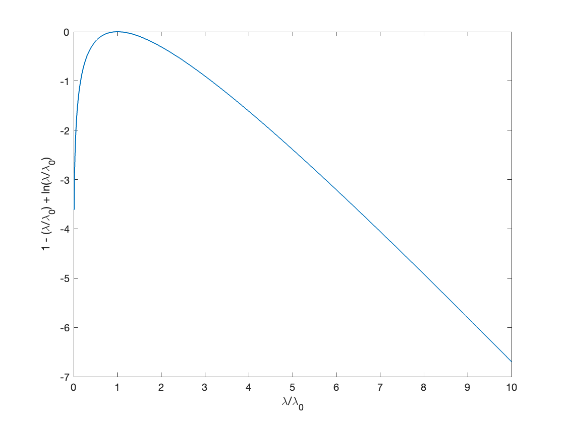
Figure 2: Plot showing $1-(\lambda/\lambda_{0})+\ln(\lambda/\lambda_{0})<0$.

Furthermore,

$$\int_{0}^{\infty}f(\lambda;c)d\lambda=\frac{c^{c}}{\lambda_{0}^{c}\Gamma(c)}\int_{0}^{\infty}\lambda^{c-1}e^{-\lambda c/\lambda_{0}}=\frac{c^{c}}{\lambda_{0}^{c}\Gamma(c)}\frac{\Gamma(c)}{(c/\lambda_{0})^{c}}=1,\,\,\forall c.$$ (B.4)

Finally, if $g(\lambda)$ is a smoothly varying function of $\lambda$, we have

$$\int_{0}^{\infty}g(\lambda)\lim_{c\to\infty}f(\lambda;c)d\lambda =\int_{0}^{\lambda_{0}-\varepsilon}g(\lambda)\lim_{c\to\infty}f(\lambda;c)d\lambda +\int_{\lambda_{0}-\varepsilon}^{\lambda_{0}+\varepsilon}g(\lambda)\lim_{c\to\infty}f(\lambda;c)d\lambda$$

$$+\int_{\lambda_{0}+\varepsilon}^{\infty}g(\lambda)\lim_{c\to\infty}f(\lambda;c)d\lambda$$ (B.5)

$$\approx g(\lambda_{0})\int_{\lambda_{0}-\varepsilon}^{\lambda_{0}+\varepsilon}\lim_{c\to\infty}f(\lambda;c)d\lambda$$ (B.6)

$$\approx g(\lambda_{0})\int_{0}^{\infty}f(\lambda;c)d\lambda$$ (B.7)

$$\approx g(\lambda_{0}),$$ (B.8)

where (B.6) follows from (B.3), and (B.8) follows from (B.4).

Therefore,

$$\lim_{c\to\infty}f(\lambda;c)=\delta(\lambda-\lambda_{0}).$$

This result is also numerically verified (see Figure 3). ∎

Figure 3: The Gamma distribution as a function of the dispersion parameter $c$.

Appendix Appendix C Mathematical properties of Tsallis type autocorrelation function

The Tsallis type generalization of the autocorrelation may be motivated via the solution of the IVP associated with the autocorrelation function,

$$\begin{rcases}\dfrac{d\rho}{dt}=-\lambda\rho^{q},\,q\neq 1\\ \rho(0)=1\end{rcases}.$$ (C.1)

The Uhlenbeck-Ornstein model, used in Shivamoggi et al. [7] and Shivamoggi and Tuovila [8], is a special case of (C.1), corresponding to $q=1$.

The solution to the IVP (C.1) is given by

$$y=[1-\lambda(1-q)t]^{\frac{1}{1-q}}\equiv e_{q}^{-\lambda t},\qquad(e_{1}^{-\lambda t}=e^{-\lambda t})$$ (C.2)

where $\lambda$ may be interpreted as the inverse autocorrelation time. For notational simplicity, we may write

$$e_{q}^{-\lambda t}\equiv[1-\lambda\ell t]^{\frac{1}{\ell}},\qquad\ell\equiv 1-q.$$ (C.3)

Here we discuss the asymptotic properties of (C.2).

Lemma 2.

For all $t\geq 0$, the iterated limits

$$\lim_{\lambda\to\infty}\lim_{\ell\to 0}(1-\lambda\ell t)^{\frac{1}{\ell}}=\lim_{\ell\to 0}\lim_{\lambda\to\infty}(1-\lambda\ell t)^{\frac{1}{\ell}}=0$$ (C.4)

exist and commute, but the simultaneous limit

$$\lim_{\begin{subarray}{c}\lambda\to\infty\\ \ell\to 0\end{subarray}}(1-\lambda\ell t)^{\frac{1}{\ell}}$$

does not exist.

Proof.

We begin by evaluating the limit, $\ell\to 0$, first. We note that

$${\lim_{\ell\to 0}}(1-\lambda\ell t)^{\frac{1}{\ell}}=e^{-\lambda t}.$$

Therefore, for all $t\neq 0$,

$$\lim_{\lambda\to\infty}\lim_{\ell\to 0}(1-\lambda\ell t)^{\frac{1}{\ell}}=\lim_{\lambda\to\infty}e^{-\lambda t}=0.$$

On the other hand, when evaluating the limit $\lambda\to\infty$ first, we consider separately the left and right limits $\ell\to 0^{-}$ and $\ell\to 0^{+}$. When approaching $\ell\to 0^{+}$, for sufficiently large $\lambda$, we have $(1-\lambda\ell t)<0.$ Noting, $e_{q}^{-\lambda t}=\max\{0,(1-\lambda\ell t)^{\frac{1}{\ell}}\}$, we have

$$\lim_{\ell\to 0^{+}}\lim_{\lambda\to\infty}(1-\lambda\ell t)^{\frac{1}{\ell}}=0.$$

When $\ell\to 0^{-}$, we have $\frac{1}{\ell}<0$ and hence

$$\lim_{\ell\to 0^{-}}\lim_{\lambda\to\infty}\bigg{(}\frac{1}{1+\lambda\absolutevalue{\ell}t}\bigg{)}^{\absolutevalue{\frac{1}{\ell}}}=0.$$

Therefore,

$$\lim_{\ell\to 0}\lim_{\lambda\to\infty}(1-\lambda\ell t)^{\frac{1}{\ell}}=0$$

for all $t\neq 0$.

For the simultaneous limit, let $N$ be a natural number. First, consider $\ell=\frac{1}{N^{2}}$ and $\lambda=N$. Then

$$\lim_{\begin{subarray}{c}\lambda\to\infty\\ \ell\to 0\end{subarray}}(1-\lambda\ell t)^{\frac{1}{\ell}}=\lim_{N\to\infty}\bigg{(}1-\frac{t}{N}\bigg{)}^{N}=e^{t}.$$

On the other hand, if we consider $\ell=\frac{1}{N^{3}}$ and $\lambda=N$, we obtain

$$\lim_{\begin{subarray}{c}\lambda\to\infty\\ \ell\to 0\end{subarray}}(1-\lambda\ell t)^{\frac{1}{\ell}}=\lim_{N\to\infty}\bigg{(}1-\frac{t}{N^{2}}\bigg{)}^{N}=1.$$

Therefore, the simultaneous limit $\displaystyle\lim_{\begin{subarray}{c}\lambda\to\infty\\ \ell\to 0\end{subarray}}(1-\lambda\ell t)^{\frac{1}{\ell}}$ does not exist, even though both iterated limits exist and are equal.

∎

Theorem 1.

For small values of $\lambda$,

$$[1-\lambda\ell t]^{\frac{1}{\ell}}\sim 1-\lambda t.$$ (C.5)

For very large values of $\lambda$,

$$\lim_{\lambda\to\infty}\lim_{\ell\to 0}(1-\lambda\ell t)^{\frac{1}{\ell}}\sim\frac{1}{\lambda}\delta(t).$$ (C.6)

Proof.

For small values of $\lambda$, on using a first order Taylor series approximation [21], we have

$$[1-\lambda\ell t]^{\frac{1}{\ell}}\sim 1-\lambda t.$$ (C.5)

For large values of $\lambda$, we have, from Lemma 2 that, for all $t\neq 0$,

$$\lim_{\lambda\to\infty}\lim_{\ell\to 0}(1-\lambda\ell t)^{\frac{1}{\ell}}=0.$$

Furthermore, we have

$$\int_{0}^{\infty}\lim_{\lambda\to\infty}\lim_{\ell\to 0}\lambda(1-\lambda\ell t)^{\frac{1}{\ell}}dt =\int_{0}^{\infty}\lim_{\lambda\to\infty}\lambda e^{-\lambda t}dt$$ (C.7a)

$$=\lim_{\lambda\to\infty}\int_{0}^{\infty}\lambda e^{-\lambda t}dt$$ (C.7b)

$$=\lim_{\lambda\to\infty}1=1.$$ (C.7c)

∎

Appendix Appendix D Double integral of Tsallis type autocorrelation

Consider the double integral of the autocorrelation,

$$I_{q}(t)\equiv\frac{1}{2}\int_{0}^{t}\int_{0}^{t}\langle b(t^{\prime})b(t^{\prime\prime})\rangle dt^{\prime}dt^{\prime\prime}.$$ (D.1)

For a stationary process, the autocorrelation becomes

$$\langle b(t^{\prime})b(t^{\prime\prime})\rangle\equiv g(t^{\prime}-t^{\prime\prime})$$ (D.2a)

and (D.1) may then be transformed via a change of variables into the single integral

$$I_{q}(t)=\int_{0}^{t}(t-\tau)g(\tau)d\tau.$$ (D.2b)

Using the Tsallis type [12] prescription, we have

$$g(\tau)=e_{q}^{-\lambda\tau}=[1-\lambda\ell\tau]^{\frac{1}{\ell}}.$$ (D.3)

(D.1) then becomes

$$I_{q}(t)=\int_{0}^{t}(t-\tau)[1-\ell\lambda\tau]^{\frac{1}{\ell}}d\tau,$$ (D.4)

which can be evaluated exactly,

$$I_{q}(t)=\frac{t}{\lambda(1+\ell)}+\frac{1}{\lambda^{2}(1+\ell)(1+2\ell)}[1-\lambda\ell t]^{\frac{1}{\ell}+2}-\frac{1}{\lambda^{2}(1+\ell)(1+2\ell)}$$ (D.5)

for $\ell\neq 0$ $(q\neq 1)$.

Numerical evaluations demonstrate several properties of $I_{q}(t)$:

Property 1.

For $q<1$, $I_{q}(t)$ increases as $q$ increases (see Figure 4).

Property 2.

For $q>1$, $I_{q}(t)$ decreases as $\lambda$ increases (see Figure 5).

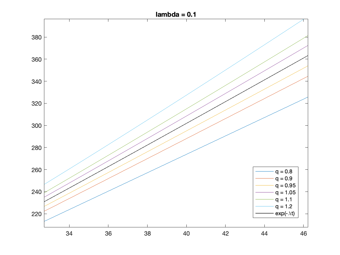
Figure 4: Plot showing $I_{q}(t)$ vs $q$. Here the parameter $\lambda=0.1$, but the behavior is unchanged when varying $\lambda$.

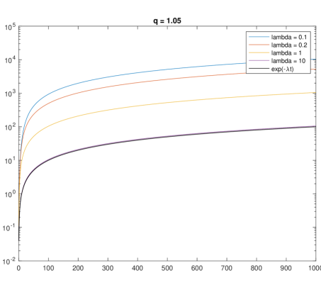
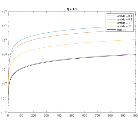
Figure 5: Plots of $I_{q}(t)$ vs $\lambda$ for $q\approx 1$.

References

- [1] R. H. Kraichnan, “Dynamics of nonlinear stochastic systems,” Journal of Mathematical Physics, vol. 2, no. 1, pp. 124–148, 1961.
- [2] R. H. Kraichnan, “Lagrangian-history closure approximation for turbulence,” The Physics of Fluids, vol. 8, no. 4, pp. 575–598, 1965.
- [3] R. H. Kraichnan, “Kolmogorov’s hypotheses and Eulerian turbulence theory,” The Physics of Fluids, vol. 7, pp. 1723–1734, 1964.
- [4] C. Y. Mou and P. B. Weichman, “Spherical model for turbulence,” Physical Review Letters, vol. 70, pp. 1101–1104, 1993.
- [5] C. Y. Mou and P. B. Weichman, “Multicomponent turbulence, the spherical limit, and non-Kolmogorov spectra,” Physical Review E, vol. 52, pp. 3738–3796, 1995.
- [6] G. L. Eyink, “Large-N limit of the “spherical model” of turbulence,” Physical Review E, vol. 49, pp. 3990–4002, 1994.
- [7] B. K. Shivamoggi, M. Taylor, and S. Kida, “On Some Mathematical Aspects of the Direct-Interaction Approximation in Turbulence Theory,” Journal of Mathematical Analysis and Applications, vol. 229, no. 2, pp. 639–658, 1999.
- [8] B. K. Shivamoggi and N. Tuovila, “Direct interaction approximation for non-Markovianized stochastic models in the turbulence problem,” Chaos, vol. 29, p. 063124, 2019.
- [9] G. E. Uhlenbeck and L. S. Ornstein, “On the Theory of the Brownian Motion,” The Physical Review, vol. 36, pp. 823–841, 1930.
- [10] I. M. Lifshits, S. A. Gredeskul, and L. A. Pastur, Introduction to the Theory of Disordered Systems. A Wiley Interscience publication, Wiley, 1988.
- [11] P. R. Weiss, “The Application of the Bethe-Peierls Method to Ferromagnetism,” Phys. Rev., vol. 74, pp. 1493–1504, 1948.
- [12] C. Tsallis, “Possible generalization of the Boltzmann-Gibbs statistics,” Journal of Statistical Physics, vol. 52, pp. 479–487, 1988.
- [13] L. C. Andrews, R. L. Phillips, B. K. Shivamoggi, J. K. Beck and M. L. Joshi, “A statistical theory for the distribution of energy dissipation in intermittent turbulence,” Physics of Fluids A, vol. 1, no. 6, pp. 999–1006, 1989.
- [14] L. C. Andrews and B. K. Shivamoggi, “The gamma distribution as a model for temperature dissipation in intermittent turbulence,” Physics of Fluids A, vol. 2, no. 1, pp. 105–110, 1990.
- [15] G. Wilk and Z. Wlodarcyzk, “Interpretation of the non-extensivity parameter in some applications of Tsallis statistics and Lèvy distributions,” Physical Review Letters, vol. 84, no. 13, pp. 2770–2773, 2000.
- [16] C. Beck, “Dynamical foundations of non-extensive statistical mechanics,” The Physical Review Letters, vol. 87, pp. 180601.1–.4, 2001.
- [17] R. Zwanzig, Nonequilibrium Statistical Mechanics. Oxford University Press, 2001.
- [18] J. B. Keller, “Stochastic equations and wave propagation in random media,” in Stochastic Processes in Mathematical Physics and Engineering (R. Bellman, ed.), no. 16 in Proceedings of Symposia in Applied Mathematics, American Mathematical Society, 1964.
- [19] R. H. Kraichnan, “Irreversible statistical mechanics of incompressible hydromagnetic turbulence,” The Physical Review, vol. 109, pp. 1407–1422, 3 1958.
- [20] R. H. Kraichnan, “The structure of isotropic turbulence at very high Reynolds numbers,” Journal of Fluid Mechanics, vol. 5, no. 4, p. 497–543, 1959.
- [21] C. Tsallis, Introduction to Nonextensive Statistical Mechanics. Springer, 2nd ed., 2023.
- [22] L. C. Andrews, Special Functions of Mathematics for Engineers. SPIE Press, 1998.