Quantum scalar field theory on equal-angular-momenta Myers-Perry-AdS black holes

Abstract

We study the canonical quantization of a massive scalar field on a five dimensional, rotating black hole space-time. We focus on the case where the space-time is asymptotically anti-de Sitter and the black hole’s two angular momentum parameters are equal. In this situation the geometry possesses additional symmetries which simplify both the mode solutions of the scalar field equation and the stress-energy tensor. When the angular momentum of the black hole is sufficiently small that there is no speed-of-light surface, there exists a Killing vector which is time-like in the region exterior to the event horizon. In this case classical superradiance is absent and we construct analogues of the usual Boulware and Hartle-Hawking quantum states for the quantum scalar field. We compute the differences in expectation values of the square of the quantum scalar field operator and the stress-energy tensor operator between these two quantum states.

I Introduction

Before compelling observational evidence demonstrated the existence of rotating black holes in our Universe, theorists had obtained not only a classical metric describing a rotating black hole [1] but also investigated quantum processes on this space-time background [2, 3]. Notably, even before the remarkable discovery that all nonextremal black holes emit thermal quantum radiation [4], it was known that quantum particles spontaneously emanate from rotating black holes [2, 3].

These profound discoveries continue, almost fifty years later, to stimulate research into the behaviour of quantum fields on rotating black hole space-times. However, any such investigation is technically extremely challenging, even though the Kerr black hole [1] is axisymmetric and the Teukolsky equation governing linear, classical perturbations of this space-time is separable [5].

Of central importance in studying quantum processes on black hole space-times is the expectation value of the stress-energy tensor (SET) operator, which encodes detailed information about the Hawking emission and governs the back-reaction of the quantum field on the space-time geometry. Computations of the SET expectation value on static, spherically symmetric black holes have been undertaken since the 1980s [6, 7, 8, 9] and have received fresh impetus in the past decade with the development of new methodologies [10, 11, 12, 13] which both improve the efficiency of the numerical calculations and permit the examination of the SET on a wider range of black hole space-times.

It is striking that, despite the long history of the subject and the deep motivation for studies of the SET expectation value, its full computation on a Kerr black hole has been performed only comparatively recently [14]. This is because the original techniques [6, 7, 8, 9] were adapted to static and spherically symmetric space-times and were not easily extended to the reduced symmetry of a rotating black hole geometry. The sophisticated methodology employed in [14] still faces formidable practical challenges, for example some four million scalar field modes are required to produce those results.

These difficulties provide compelling motivation for the study of quantum fields on alternative rotating black hole geometries which reduce the technical complexities. One line of attack is to lower the number of space-time dimensions to three. The rotating BTZ black hole [15, 16] is constructed by identifying points in three-dimensional anti-de Sitter (AdS) space-time. As a result, the SET expectation value of a quantum scalar field on this background can be found using the method of images [17]. The consequent SET expectation value is sufficiently simple in form to enable the back-reaction of the quantum field on the space-time to be studied in depth [18, 19].

Naively, one would anticipate that increasing the number of space-time dimensions only aggravates the problem of the complexity of rotating black hole geometries. However, when the number of space-time dimensions is odd, there exist rotating black hole metrics with enhanced symmetries [20]. Black holes in $2N+3$ space-time dimensions have $N+1$ independent angular momentum parameters [21, 22] and the augmented symmetry arises on setting these parameters to be equal.

Our principal concept is therefore to explore quantum scalar field theory on these equal-angular-momenta higher dimensional black holes, anticipating that the additional symmetry will ameliorate some of the technical difficulties of working on a four-dimensional Kerr black hole. However, as well as computational challenges, there remain additional complexities in studying quantum field theory on rotating space-times.

Central to these are the subtleties which arise in the definition of suitable quantum states on rotating black holes. The Unruh state [23] is the most relevant for the study of Hawking radiation; it is the analogue on an eternal black hole geometry of the quantum state pertinent to a black hole formed by gravitational collapse. Construction of the Unruh state on a rotating black hole space-time is uncontroversial [24]; indeed it is in this state that the SET expectation value has been computed [14]. Nonetheless, the Unruh state does not preserve all the symmetries of the underlying space-time (in particular, it is not symmetric under the simultaneous inversion of the time and azimuthal angular coordinate). For this reason, both the original methods [6, 7, 8, 9] for computing the SET expectation value and a more recent approach [12] have used the Hartle-Hawking state [25]. This latter state is particularly well-adapted to SET computations, being a thermal equilibrium state, regular across both the future and past event horizons, and respecting the symmetries of the underlying black hole geometry. Furthermore, since differences in expectation values between two quantum states do not require renormalization, they are comparatively straightforward to compute.

Unfortunately, the Hartle-Hawking state does not exist on a Kerr black hole background for a quantum scalar field [26]; there is no state representing a Kerr black hole in equilibrium with a thermal heat bath at the Hawking temperature. This can be understood heuristically by considering the toy model of a rotating thermal state in Minkowski space-time [27]. In unbounded Minkowski space-time, a rigidly-rotating thermal state does not exist for a quantum scalar field [27], but such a state can be constructed if Minkowski space-time is bounded by an infinite cylinder, symmetrical about the axis of rotation, of sufficiently small radius that there is no speed-of-light surface [27]. The speed-of-light surface is the surface on which rigidly-rotating observers must travel at the speed of light. Correspondingly, if a Kerr black hole is surrounded by a perfectly reflecting mirror inside the speed-of-light surface, then a Hartle-Hawking state can be defined for a quantum scalar field [28]. One disadvantage of introducing a reflecting boundary in order to construct rotating thermal states is that Casimir divergences result on the boundary [27, 29].

The issue of Casimir divergences can be circumventing by considering black holes which are asymptotically AdS rather than asymptotically flat. For example, the BTZ black hole [15, 16] does not have a speed-of-light surface, enabling a well-defined Hartle-Hawking state. Indeed, this is the state for which the SET expectation values are computed in [17]. In four space-time dimensions, Kerr-AdS black holes [30] do not have a speed-of-light surface if their angular momentum is sufficiently small. In this case there are no superradiant instabilities [31, 32] and the black hole can be in thermal equilibrium with a heat bath at the Hawking temperature [33]. In the absence of a speed-of-light surface, the space-time possesses a Killing vector which is timelike outside the event horizon. This Killing vector plays a central role in the rigorous construction of the quantum scalar field Hartle-Hawking state on a four-dimensional stationary black hole without a speed-of-light surface [34].

We are therefore motivated to study quantum fields on asymptotically AdS equal-angular-momenta black holes. While such black holes have enhanced symmetry in any number of odd space-time dimensions, for simplicity we consider only the five-dimensional case. This has the advantage that there are no “ultra-spinning” instabilities [35]. We assume that the angular momentum of the black hole is sufficiently small that there is no speed-of-light surface. In this case there is an elegant argument [33] that the black holes are classically stable (see also [20, 36, 37, 38, 39] for studies of the gravitational perturbations of these black holes, confirming the absence of instabilities). The arguments in [33], valid for a general five-dimensional asymptotically AdS rotating black hole without speed-of-light surface, reveal that the black holes we study can be in thermal equilibrium with a heat bath at the Hawking temperature. Accordingly, we conjecture that it will be possible to construct a Hartle-Hawking state in this scenario.

While the Hartle-Hawking state is our primary interest, we also seek to define a second quantum state, in order to study differences in expectation values between two quantum states without recourse to renormalization. The existence of an Unruh-like state on asymptotically-AdS black holes is complex. For an asymptotically-AdS black hole formed by gravitational collapse, the nature of the quantum state at late times depends on the details of the collapse process and the boundary conditions applied to the quantum field far from the black hole [40, 41, 42]. On an eternal, asymptotically-AdS black hole, if reflecting boundary conditions are applied to the quantum field (as will be the case in our study), then it is not possible to define an Unruh-like state.

We therefore seek an analogue of the Boulware vacuum [43], in other words a zero temperature state. For a nonrotating black hole, this state is as empty as possible as seen by a static observer far from the black hole, although it is divergent at the event horizon [44]. On Kerr space-time, for a quantum scalar field there is no corresponding state which is empty at both future and past null infinity [24]. This is because a rotating black hole spontaneously emits particles even if its temperature is zero [2, 3]. For a bosonic field (such as quantum scalar field on which we focus in this paper), this spontaneous nonthermal quantum emission occurs in precisely those field modes which are subject to classical superradiance [45]. For a scalar field, such superradiant modes are absent on Kerr-AdS black holes when reflective boundary conditions are applied [46]. Similar conclusions can be drawn for a scalar field on the asymptotically-AdS equal-angular-momenta black holes [47]. We therefore expect that a Boulware-like state can be constructed in our set-up.

Our paper is structured as follows. In Sec. II we review the geometry of five dimensional, equal-angular-momenta black holes in asymptotically AdS space-time, paying particular attention to the symmetries of the geometry. The properties of a classical massive scalar field on this background are examined in Sec. III, where we derive separable mode solutions of the scalar field equation. In Sec. IV we turn to the canonical quantization of the scalar field, constructing analogues of the standard Boulware and Hartle-Hawking states. Differences in expectation values of the square of the quantum scalar field and the SET between these two states are computed in Sec. V. Finally, Sec. VI contains further discussion and our conclusions.

II Equal-angular-momenta black holes in five dimensions

The higher-dimensional, asymptotically flat, rotating Myers-Perry black hole solutions [21, 22] of the vacuum Einstein equations are generalizations of the four-dimensional Kerr metric [1]. Including a cosmological constant further complicates the metric in higher dimensions [48, 49, 50]. Working in five space-time dimensions, the general rotating black hole geometry [48] has, in addition to the cosmological constant, a mass parameter and two independent angular momentum parameters. Setting these two angular momentum parameters equal results in a space-time geometry which has enhanced symmetry [20] and these equal-angular-momenta black holes are the focus of our study.

In terms of the coordinates $(t,r,\theta,\phi,\psi)$ which are adapted to the enhanced symmetry, the black hole metric takes the form [20]:

$$ds^{2}= -f(r)^{2}dt^{2}+g(r)^{2}dr^{2}+\frac{r^{2}}{4}\left[d\theta^{2}+\sin^{2}\theta\,d\varphi^{2}\right]$$

$$+h(r)^{2}\left[d\psi+\frac{1}{2}\cos\theta\,d\varphi-\Omega(r)\,dt\right]^{2},$$ (1a)

where $$\theta\in[0,\pi) \varphi\in[0,4\pi) \psi\in[0,2\pi)$$, , , and

$$g(r)^{2} =\left(1+\frac{r^{2}}{L^{2}}-\frac{2M}{r^{2}}+\frac{2Ma^{2}}{r^{2}L^{2}}+\frac{2Ma^{2}}{r^{4}}\right)^{-1},$$ (1b)

$$h(r)^{2} =r^{2}\left(1+\frac{2Ma^{2}}{r^{4}}\right),$$ (1c)

$$\Omega(r) =\frac{2Ma}{r^{2}h(r)^{2}},$$ (1d)

$$f(r) =\frac{r}{g(r)h(r)}.$$ (1e)

Throughout this paper, the space-time signature is $(-,+,+,+,+)$ and we use units in which $8\pi G=c=\hbar=k_{B}=1$. The constants in the metric (1) have the following interpretation: $M$ is the mass parameter, $a$ is the angular momentum parameter, and $L$ is the AdS length scale, related to the cosmological constant $\Lambda$ by $\Lambda=-6L^{-2}$. Taking the limit $L\rightarrow\infty$ gives an asymptotically flat black hole, considered (using different coordinates) in [51, 52]. The mass $E$ and angular momentum $J$ of the black hole are given in terms of the parameters $M$ and $J$ by [53]:

$$E=\frac{\pi^{2}M}{2}\left(3+\frac{a^{2}}{L^{2}}\right),\qquad J=2\pi^{2}aM.$$ (2)

The square root of minus the determinant of the metric (1) is

$${\mathsf{g}}={\sqrt{-\det g_{\mu\nu}}}=\frac{1}{4}r^{3}\sin\theta.$$ (3)

The inverse metric $g^{\mu\nu}$ has the following nonzero components:

$$g^{tt} =-f(r)^{-2},$$ (4a)

$$g^{t\psi} =-\Omega(r)f(r)^{-2},$$ (4b)

$$g^{rr} =g(r)^{-2},$$ (4c)

$$g^{\theta\theta} =4r^{-2},$$ (4d)

$$g^{\varphi\varphi} =4r^{-2}\csc^{2}\theta,$$ (4e)

$$g^{\varphi\psi} =-2r^{-2}\cot\theta\csc\theta,$$ (4f)

$$g^{\psi\psi} =r^{-2}\cot^{2}\theta+h(r)^{-2}-\Omega(r)^{2}f(r)^{-2}.$$ (4g)

By evaluating the Kretschmann scalar $R_{\alpha\beta\gamma\delta}R^{\alpha\beta\gamma\delta}$, where $R_{\alpha\beta\gamma\delta}$ is the Riemann tensor, we find that the metric (1) has a singularity at $r=0$. The Penrose diagram for this black hole geometry can be found in Fig. 1 [54].

Figure 1: Penrose diagram of an equal-angular momentum, asymptotically-anti-de Sitter, Myers-Perry black hole [54]. Dotted lines denote horizons. The event horizon is located at $r=r_{+}$, and inner horizon at $r=r_{-}$. Null infinity is the time-like surface at $r=\infty$, while there is a curvature singularity at $r=0$ (denoted by the dashed lines).

It is striking that the black hole metric (1) essentially depends only on the radial coordinate $r$. The angular coordinates $(\theta,\varphi,\psi)$ are coordinates on the three-sphere ${\mathbb{S}}^{3}$, here written as an ${\mathbb{S}}^{1}$ fibre (parameterized by the angle $\psi$) over ${\mathbb{CP}}^{1}$ [20]. With this interpretation, the part of the metric

$$\frac{r^{2}}{4}\left[d\theta^{2}+\sin^{2}\theta\,d\varphi^{2}\right]$$ (5)

corresponds to the Fubini-Study metric on ${\mathbb{CP}}^{1}$, while

$$\frac{1}{2}\cos\theta\,d\varphi$$ (6)

is the Kähler form on ${\mathbb{CP}}^{1}$ [20].

The metric (1) possesses the following independent Killing vectors [51, 55]:

$${\mathcal{V}}_{1} =\frac{\partial}{\partial t},\qquad{\mathcal{V}}_{2}=\frac{\partial}{\partial\varphi},\qquad{\mathcal{V}}_{3}=\frac{\partial}{\partial\psi},$$ (7a)

$${\mathcal{V}}_{4} =2\cos\varphi\frac{\partial}{\partial\theta}-2\sin\varphi\cot\theta\frac{\partial}{\partial\varphi}+\sin\varphi\csc\theta\frac{\partial}{\partial\psi},$$ (7b)

$${\mathcal{V}}_{5} =-2\sin\varphi\frac{\partial}{\partial\theta}-2\cos\varphi\cot\theta\frac{\partial}{\partial\varphi}+\cos\varphi\csc\theta\frac{\partial}{\partial\psi}.$$ (7c)

In addition, the metric (1) has “hidden symmetries” (Killing-Yano tensors) [56, 57] which we do not need to consider in detail, but which become manifest in the separability of the Klein-Gordon equation, as studied in Sec. III.

Horizons occur at the zeros of the polynomial $g(r)^{-2}$. This gives a cubic in $x=r^{2}$:

$$x^{3}+L^{2}x^{2}+2M\left(a^{2}-L^{2}\right)x+2a^{2}L^{2}M=0,$$ (8)

the discriminant of which is always positive, so that there are three real roots, which we will denote by $r_{0}^{2}$, $r_{-}^{2}$ and $r_{+}^{2}$. One of these roots (taken to be $r_{0}^{2}$ without loss of generality) is negative, and the other two are positive. The larger of the two positive roots, $r_{+}^{2}$, corresponds to the (outer) event horizon of the black hole, while $r_{-}^{2}$ corresponds to the inner horizon. The event horizon radius $r_{+}$ is given by

$$r_{+}^{2}=\frac{1}{3}\Bigg{\{}2{\sqrt{\mathfrak{A}}}\cos\left(\frac{1}{3}\cos^{-1}\left[-\frac{{\sqrt{\mathfrak{B}}}}{{\mathfrak{A}}^{\frac{3}{2}}}\right]\right)-L^{2}\Bigg{\}},$$ (9a)

where

$${\mathfrak{A}} =L^{4}-6M\left(a^{2}-L^{2}\right),$$

$${\mathfrak{B}} =L^{6}+9L^{2}M\left(2a^{2}+L^{2}\right).$$ (9b)

Using (8), we can write the mass parameter $M$ in terms of $a$, $L$ and $r_{+}$:

$$M=-\frac{r_{+}^{4}\left(r_{+}^{2}+L^{2}\right)}{2\left(r_{+}^{2}\left[a^{2}-L^{2}\right]+a^{2}L^{2}\right)}.$$ (10)

Substituting for $M$ in the cubic (8) then gives a quadratic having roots $x=r_{-}^{2}$ and $x=r_{0}^{2}$:

$$x^{2}+\left(r_{+}^{2}+L^{2}\right)x+\frac{a^{2}L^{2}r_{+}^{2}\left(r_{+}^{2}+L^{2}\right)}{r_{+}^{2}\left(a^{2}-L^{2}\right)+a^{2}L^{2}}=0.$$ (11)

The roots of this quadratic are then:

$$r_{-}^{2} =-\frac{1}{2}\left(r_{+}^{2}+L^{2}\right)$$

$$\quad\times\left[1-{\sqrt{\frac{a^{2}\left(L^{2}-r_{+}^{2}\right)^{2}-L^{2}r_{+}^{2}\left(r_{+}^{2}+L^{2}\right)}{\left(r_{+}^{2}\left[a^{2}-L^{2}\right]+a^{2}L^{2}\right)\left(r_{+}^{2}+L^{2}\right)}}}\right],$$ (12a)

$$r_{0}^{2} =-\frac{1}{2}\left(r_{+}^{2}+L^{2}\right)$$

$$\quad\times\left[1+{\sqrt{\frac{a^{2}\left(L^{2}-r_{+}^{2}\right)^{2}-L^{2}r_{+}^{2}\left(r_{+}^{2}+L^{2}\right)}{\left(r_{+}^{2}\left[a^{2}-L^{2}\right]+a^{2}L^{2}\right)\left(r_{+}^{2}+L^{2}\right)}}}\right].$$ (12b)

The following relations involving the roots of the cubic (8) will be useful in Sec. III.2.2:

$$r_{+}^{2}+r_{-}^{2}+r_{0}^{2} =~{}-L^{2},$$ (13a)

$$r_{+}^{2}r_{-}^{2}+r_{-}^{2}r_{0}^{2}+r_{0}^{2}r_{+}^{2} =~{}2M\left(a^{2}-L^{2}\right),$$ (13b)

$$r_{+}^{2}r_{-}^{2}r_{0}^{2} =~{}-2a^{2}ML^{2},$$ (13c)

and from these we can write $$M a^{2}$$ and as follows:

$$a^{2} =~{}\frac{r_{+}^{2}r_{-}^{2}r_{0}^{2}\left(r_{+}^{2}+r_{-}^{2}+r_{0}^{2}\right)}{\left(r_{+}^{2}+r_{-}^{2}\right)\left(r_{-}^{2}+r_{0}^{2}\right)\left(r_{0}^{2}+r_{+}^{2}\right)},$$ (13d)

$$M =~{}\frac{\left(r_{+}^{2}+r_{-}^{2}\right)\left(r_{-}^{2}+r_{0}^{2}\right)\left(r_{0}^{2}+r_{+}^{2}\right)}{2\left(r_{+}^{2}+r_{-}^{2}+r_{0}^{2}\right)^{2}}.$$ (13e)

The outer and inner horizons coincide (so that $r_{+}=r_{-}$ and the black hole becomes extremal) when the spin parameter $a=a_{\rm{ext}}$, which is given, in terms of the event horizon radius, by

$$a_{\rm{ext}}^{2}=\frac{L^{2}r_{+}^{2}\left(2r_{+}^{2}+L^{2}\right)}{2\left(r_{+}^{2}+L^{2}\right)^{2}}.$$ (14)

For values of the spin parameter $a$ above $a_{\rm{ext}}$, there is a naked singularity.

Since the black hole is rotating, it possesses an ergosphere, inside which an observer cannot remain at rest relative to infinity. The boundary of this region is the stationary limit surface, given by

$$0=-g_{tt}=f(r)^{2}-h(r)^{2}\Omega(r)^{2}=\frac{r^{2}}{L^{2}}-\frac{2M}{r^{2}}+1.$$ (15)

This has two roots for $x=r^{2}$, only one of which is positive. This gives the radius $r_{{\rm{S}}}$ of the stationary limit surface:

$$r_{{\rm{S}}}^{2}=\frac{L^{2}}{2}\left[{\sqrt{1+\frac{8M}{L^{2}}}}-1\right].$$ (16)

Thus, unlike the situation in four-dimensional Kerr space-time, the radius of the stationary limit surface is a constant and does not depend on any of the angular coordinates. This is a result of the enhanced symmetry of equal-angular-momenta black holes. Surprisingly, the radius (16) is independent of the spin parameter $a$ and depends only on the mass parameter $M$ and the AdS length scale $L$.

The event horizon at $r=r_{+}$ is a Killing horizon for the Killing vector

$${\mathcal{V}}_{\rm{+}}=\frac{\partial}{\partial t}+\Omega_{\rm{+}}\frac{\partial}{\partial\psi},$$ (17)

where $\Omega_{+}$ is the angular speed of the event horizon, given by [20]

$$\Omega_{+}=\Omega(r_{+})=\frac{2Ma}{r_{+}^{4}+2Ma^{2}},$$ (18)

and has surface gravity $\kappa_{+}$ given by

$$\kappa_{+}=\frac{r_{+}^{2}L^{2}\left(2r_{+}^{2}+L^{2}\right)-2a^{2}\left(r_{+}^{2}+L^{2}\right)^{2}}{r_{+}^{2}L^{3}{\sqrt{r_{+}^{2}\left(L^{2}-a^{2}\right)-a^{2}L^{2}}}}.$$ (19)

Kruskal coordinates regular across the event horizon can be constructed by first defining a corotating coordinate $\psi_{+}$:

$$\psi_{+}=\psi-\Omega_{+}t,$$ (20)

in terms of which the metric (1) becomes

$$ds^{2}= -f(r)^{2}dt^{2}+g(r)^{2}dr^{2}+\frac{r^{2}}{4}\left[d\theta^{2}+\sin^{2}\theta\,d\varphi^{2}\right]$$

$$+h(r)^{2}\left[d\psi_{+}+\frac{1}{2}\cos\theta\,d\varphi-\left\{\Omega(r)-\Omega_{+}\right\}dt\right]^{2}.$$ (21)

Next, the “tortoise” coordinate $r_{\star}$ is given by [20]

$$\frac{dr_{\star}}{dr}=\frac{g(r)}{f(r)}=\frac{1}{r}g(r)^{2}h(r),$$ (22)

and the usual double-null coordinates are

$$u=t-r_{\star},\qquad v=t+r_{\star}.$$ (23)

We then define the Kruskal coordinates $U$, $V$ as:

$$U=-\frac{1}{\kappa_{+}}e^{-\kappa_{+}u},\qquad V=\frac{1}{\kappa_{+}}e^{\kappa_{+}v}.$$ (24)

In terms of these Kruskal coordinates, the metric is

$$ds^{2}_{\rm{K}}= -\frac{f(r)^{2}}{\kappa_{+}^{2}UV}\,dU\,dV+\frac{r^{2}}{4}\left[d\theta^{2}+\sin^{2}\theta\,d\varphi^{2}\right]$$

$$+h(r)^{2}\left[d\psi_{+}+\frac{1}{2}\cos\theta\,d\varphi\right.$$

$$\left.\qquad-\frac{1}{2\kappa_{+}}\left\{\Omega(r)-\Omega_{+}\right\}\left(\frac{dV}{V}+\frac{dU}{U}\right)\right]^{2}.$$ (25)

Close to the event horizon, the Killing vector ${\mathcal{V}}_{+}$ (17) is timelike. It becomes spacelike on the speed-of-light surface, where

$$0=g_{tt}+2\Omega_{+}g_{t\psi}+\Omega_{+}^{2}g_{\psi\psi}.$$ (26)

This gives a simple quadratic equation for $x=r^{2}$:

$$\left(L^{2}\Omega_{+}^{2}-1\right)x^{2}-L^{2}x+2ML^{2}\left(1-a\Omega_{+}\right)^{2}=0.$$ (27)

Examining the discriminant of this quadratic, we find that real solutions for $x$ exist only when $\Omega_{+}L>1$. In this case there is a single positive solution $r_{\rm{L}}^{2}$:

$$r_{\rm{L}}^{2}=\frac{1}{2\left(\Omega_{+}^{2}L^{2}-1\right)}\left[L^{2}\right.\\ \left.+{\sqrt{L^{4}-8ML^{2}\left(1-a\Omega_{+}\right)^{2}\left(\Omega_{+}^{2}L^{2}-1\right)}}\right].$$ (28)

In a four-dimensional Kerr space-time, the speed-of-light surface has a complicated structure and its radius depends on the angular coordinate $\theta$ [28]. In our set-up, the radius $r_{\rm{L}}$ of the speed-of-light surface is independent of all the angular variables. When $\Omega_{+}<L^{-1}$, the speed-of-light surface is absent; this is the situation in which we are interested. We can find the maximum value of the spin parameter $a$ for which there is no speed-of-light surface as follows. We first use the cubic (8) to write the mass parameter $M$ in terms of the event horizon radius $r_{+}$ and $\Omega_{+}$ [20]:

$$M=\frac{r_{+}^{2}\left(1+r_{+}^{2}/L^{2}\right)}{2\left(1+r_{+}^{2}/L^{2}-r_{+}^{2}\Omega_{+}^{2}\right)},$$ (29)

and then the angular speed of the event horizon $\Omega_{+}$ (18) takes the form

$$\Omega_{+}=a\left(\frac{1}{L^{2}}+\frac{1}{r_{+}^{2}}\right).$$ (30)

Thus $\Omega_{+}=L^{-1}$ when $a=a_{\rm{max}}$, where

$$a_{\rm{max}}=\frac{r_{+}^{2}L}{r_{+}^{2}+L^{2}}.$$ (31)

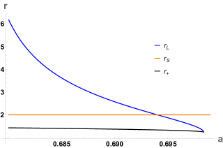
Figure 2: The locations of the event horizon $r_{+}$ (9), stationary limit surface $r_{{\rm{S}}}$ (16) and speed-of-light surface $r_{\rm{L}}$ (28) as functions of the spin parameter $a$ for fixed mass parameter $M=10L^{2}$. We use units in which $L=1$.

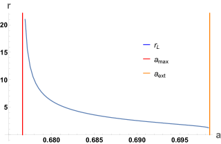
Figure 3: Location of the speed-of-light surface $r_{\rm{L}}$ (28) as a function of the spin parameter $a$ for fixed mass parameter $M=10L^{2}$. The vertical lines give the values of $a_{\rm{max}}$ (31) and $a_{\rm{ext}}$ (14). We use units in which $L=1$.

Our equal-angular-momenta black hole space-time therefore has a “shell-like” structure, with three key surfaces at constant values of the radial coordinate $r$, namely: the event horizon $r=r_{+}$ (9), the stationary limit surface $r=r_{\rm{S}}$ (16) and the speed-of-light surface $r=r_{\rm{L}}$ (28). For fixed values of the mass parameter $M$ and AdS length $L$, the location of the stationary limit surface (16) is independent of the spin parameter $a$, but the event horizon radius and speed-of-light surface (if it exists) depend on $a$.

In Fig. 2 we show these three radii as functions of $a$ for fixed $M=10L^{2}$, using units in which $L=1$ (we shall use these units for the rest of the paper). The behaviour is qualitatively similar for other values of $M$. The orange line gives the value of $r_{\rm{S}}$ (16), which is independent of the spin parameter $a$. The black line is the event horizon radius $r_{+}$ (9), which decreases slowly as $a$ increases for the range of values of $a$ shown in the plot. The blue curve is the location of the speed-of-light surface $r_{\rm{L}}$ (28). This changes rapidly with varying $a$ and decreases as $a$ increases. When $a=a_{\rm{ext}}$, we find that $r_{+}=r_{\rm{L}}$ and the speed-of-light surface coincides with the event horizon. For sufficiently large values of $a$ (below $a_{\rm{ext}}$) the speed-of-light surface lies inside the stationary limit surface; similar behaviour is seen near the equatorial plane for near-extremal Kerr black holes [28]. The behaviour of $r_{\rm{L}}$ on decreasing $a$ further can be seen in Fig. 3. In particular, $r_{\rm{L}}$ increases rapidly as $a$ decreases, and the speed-of-light surface moves away from the black hole event horizon. There is an asymptote in $r_{\rm{L}}$ as $a\rightarrow a_{\rm{max}}$; below this value of $a$ there is no speed-of-light surface.

For the remainder of this paper we shall be concerned only with values of $0<a<a_{\rm{max}}$, so that the speed-of-light surface is absent. In this situation the Killing vector ${\mathcal{V}}_{+}$ (17) is timelike everywhere outside the event horizon. This will be important for the quantization of the scalar field in Sec. IV.

III Classical scalar field

We consider a scalar field $\Phi$ propagating on the background geometry discussed in Sec. II and satisfying the Klein-Gordon equation

$$\left[\Box-\left(\mu^{2}+\xi R\right)\right]\Phi=0,$$ (32)

where $\Box=\nabla_{\alpha}\nabla^{\alpha}$ with $\nabla_{\alpha}$ the usual covariant derivative, $\mu$ is the mass of the scalar field, and $\xi$ is a constant coupling the scalar field to the Ricci scalar $R$ of the geometry. In five space-time dimensions, the scalar field is minimally coupled for $\xi=0$ and conformally coupled when $\xi=3/16$. Since the Ricci scalar $R=-20/L^{2}$ is a constant for equal-angular-momenta black holes, we define a constant $\nu$ (the scalar field “effective mass”) by

$$\nu^{2}=\mu^{2}+\xi R.$$ (33)

The classical SET for the scalar field is [58]

$$T_{\alpha\beta} =\left(1-2\xi\right)\Phi_{;\alpha}\Phi_{;\beta}+\left(2\xi-\frac{1}{2}\right)g_{\alpha\beta}g^{\rho\sigma}\Phi_{;\rho}\Phi_{;\sigma}$$

$$\qquad-2\xi\Phi\Phi_{;\alpha\beta}+2\xi g_{\alpha\beta}\Phi\Box\Phi$$

$$\qquad+\xi\left(R_{\alpha\beta}-\frac{1}{2}Rg_{\alpha\beta}\right)\Phi^{2}-\frac{1}{2}g_{\alpha\beta}\mu^{2}\Phi^{2}$$

$$=\left(1-2\xi\right)\Phi_{;\alpha}\Phi_{;\beta}-2\xi\Phi\Phi_{;\alpha\beta}$$

$$\qquad+\left(2\xi-\frac{1}{2}\right)g_{\alpha\beta}g^{\rho\sigma}\Phi_{;\rho}\Phi_{;\sigma}$$

$$\qquad+\frac{1}{2}\left(4\xi-1\right)g_{\alpha\beta}\mu^{2}\Phi^{2}+\xi Rg_{\alpha\beta}\left(2\xi-\frac{3}{10}\right)\Phi^{2},$$ (34)

where a semicolon ; denotes a covariant derivative, and in the second equality we have used the scalar field equation (32) and the fact that $R_{\alpha\beta}=Rg_{\alpha\beta}/5$ for the equal-angular-momenta black holes. Therefore, while solutions of the scalar field equation (32) depend on the constants $\mu^{2}$ and $\xi$ only through the combination $\nu$ (33), the SET (34) depends on $\mu^{2}$ and $\xi$ separately.

The scalar field equation (32) is separable [51, 59, 60, 20, 61], and we seek mode solutions of the form:

$$\Phi(t,r,\theta,\varphi,\psi)=e^{-i\omega t}e^{ip\psi}X(r)Y(\theta,\varphi),$$ (35)

where $X(r)$ and $Y(\theta,\varphi)$ are, respectively, the radial and angular functions. The constant $\omega$ is the frequency of the mode, and $p$ is the azimuthal quantum number. Since $\psi\in[0,2\pi)$, we have $p\in{\mathbb{Z}}$.

In this section we review the angular and radial equations. Since we are only considering black holes with $\Omega_{+}L<1$ the classical scalar field modes we consider are linearly stable [20, 62].

III.1 Angular equation

Substituting the separable mode ansatz (35) for the scalar field into the equation (32) and separating variables, the resulting equation for the angular function $Y(\theta,\varphi)$ can be written as

$$0=\frac{\partial^{2}Y}{\partial\theta^{2}}+\cot\theta\frac{\partial Y}{\partial\theta}-ip\cot\theta\csc\theta\frac{\partial Y}{\partial\varphi}+\csc^{2}\theta\frac{\partial^{2}Y}{\partial\varphi^{2}}\\ -\frac{1}{4}p^{2}Y\cot^{2}\theta+\lambda Y,$$ (36)

where $\lambda$ is a separation constant. We require $Y(\theta,\varphi)$ to be regular at the poles $\theta=0,\pi$, and to be periodic in $\varphi$ with period $4\pi$.

There are several different (but equivalent) representations of the angular functions. First, Eq. (36) is the equation satisfied by a charged scalar field on ${\mathbb{CP}}^{1}$, having charge $p$ and with the gauge potential (6) [20]. On ${\mathbb{CP}}^{1}$, the angular functions $Y(\theta,\varphi)$ are monopole harmonics [63, 64].

Second, the angular function $Y(\theta,\varphi)$ can further be separated as follows:

$$Y(\theta,\varphi)=e^{im\varphi}{\widetilde{Y}}(\theta).$$ (37)

Since $\varphi\in[0,4\pi)$, we have that $2m\in{\mathbb{Z}}$. The resulting equation for ${\widetilde{Y}}(\theta)$ can be cast into the form of a hypergeometric equation, with the solutions regular at $\theta=0,\pi$ given in terms of Jacobi polynomials [51, 59] (note that [51, 59] use a different coordinate system to the one employed here, so their angular equation is modified in our case).

We shall find it more convenient to use a third representation, in which the angular functions $Y(\theta,\varphi)$ are given by spin-weighted spherical harmonics (see, for example, [65, 66, 67, 68, 69, 70, 71] for a selection of the extensive references on these, and [70, 71] for longer bibliographies). We compare (36) with the governing equation for spin-weighted spherical harmonics ${}_{s}Y_{\ell}^{n}(\theta,\varphi)$ having spin $s$, total angular momentum quantum number $\ell$ and azimuthal quantum number $n$ [68, 70, 71]:

$$0=\frac{\partial^{2}{}_{s}Y_{\ell}^{n}}{\partial\theta^{2}}+\cot\theta\frac{\partial{}_{s}Y_{\ell}^{n}}{\partial\theta}+2is\cot\theta\csc\theta\frac{\partial{}_{s}Y_{\ell}^{n}}{\partial\varphi}\\ +\csc^{2}\theta\frac{\partial^{2}{}_{s}Y_{\ell}^{n}}{\partial\varphi^{2}}-s^{2}{}_{s}Y_{\ell}^{n}\cot^{2}\theta+\left[\ell^{2}+\ell-s^{2}\right]{}_{s}Y_{\ell}^{n}.$$ (38)

Here, $s$ is a (positive or negative) integer or half-integer, $\ell=|s|,|s|+1,|s|+2,\ldots$ is a positive integer or half-integer and $m=-\ell,-\ell+1,\ldots,\ell-1,\ell$ is also an integer or half-integer (taking both positive and negative values). Comparing (36, 38), we see that the spin $s$ is related to the quantum number $p$ by

$$s=-\frac{p}{2},$$ (39)

and the separation constant $\lambda$ is given by

$$\lambda=\ell^{2}+\ell-s^{2}=\ell^{2}+\ell-\frac{1}{4}p^{2}.$$ (40)

Using the further separation (37), we may identify $m=n$. The advantage of working with spin-weighted spherical harmonics is the existence of addition theorems [72] for sums over the azimuthal quantum number $m$, which will enable us, in Sec. V, to simplify the expressions for the square of the scalar field and SET for the quantum scalar field. The relevant addition theorems are summarized in App. A.

The standard normalization for the spin-weighted spherical harmonics having integer spin $s$ is

$$\int_{\varphi=0}^{2\pi}\int_{\theta=0}^{\pi}{}_{s}Y_{\ell}^{m*}(\theta,\varphi){}_{s^{\prime}}Y_{\ell^{\prime}}^{m^{\prime}}(\theta,\varphi)\,\sin\theta\,d\theta\,d\varphi\\ =\delta_{ss^{\prime}}\delta_{\ell\ell^{\prime}}\delta_{mm^{\prime}}.$$ (41)

We use this normalization (so that the addition theorems in App. A apply), but since we have $\varphi\in[0,4\pi)$ rather than $\varphi\in[0,2\pi)$, our normalization is

$$\int_{\varphi=0}^{4\pi}\int_{\theta=0}^{\pi}{}_{s}Y_{\ell}^{m*}(\theta,\varphi){}_{s^{\prime}}Y_{\ell^{\prime}}^{m^{\prime}}(\theta,\varphi)\,\sin\theta\,d\theta\,d\varphi\\ =2\delta_{ss^{\prime}}\delta_{\ell\ell^{\prime}}\delta_{mm^{\prime}}.$$ (42)

This normalization condition is valid for half-integer as well as integer spin.

III.2 Radial equation

We next describe the radial equation in two forms: the first is a Schrödinger-like equation [20] and is useful for defining an orthonormal basis of field modes for the canonical quantization of the scalar field in Sec. IV; while the second involves a Heun equation [73, 61, 74, 62] and is useful for our numerical computations in Sec. V.

III.2.1 Potential form

The radial equation resulting from substituting the separable mode ansatz (35) into the scalar field equation (32) is

$$0=X^{\prime\prime}(r)+\left[\frac{3}{r}-\frac{2g^{\prime}(r)}{g(r)}\right]X^{\prime}(r)\\ +g(r)^{2}\left[\frac{\left\{\omega-p\Omega(r)\right\}^{2}}{f(r)^{2}}-\frac{p^{2}}{h(r)^{2}}-\frac{4\lambda}{r^{2}}-\nu^{2}\right]X(r),$$ (43)

where $\lambda$ is the separation constant (40) and $\nu^{2}$ is given in (33). Following [20], we use the “tortoise” coordinate $r_{\star}$ given by (22). Near the event horizon, as $r\rightarrow r_{+}$, we have $g(r)/f(r)\sim{\mathcal{O}}(r-r_{+})^{-1}$ and hence $r_{\star}\rightarrow-\infty$, while, as $r\rightarrow\infty$, since $g(r)/f(r)\sim{\mathcal{O}}(r^{-2})$, by a suitable choice of integration constant, we may take $r_{\star}\rightarrow 0$. Defining a new radial function ${\widetilde{X}}(r)$ by

$$X(r)=\frac{{\widetilde{X}}(r_{\star})}{r{\sqrt{h(r)}}},$$ (44)

the radial equation (43) becomes

$$\frac{d^{2}{\widetilde{X}}}{dr_{\star}^{2}}+V(r){\widetilde{X}}=0,$$ (45)

where the potential $V(r)$ is given by [20]

$$V(r)=\left[\omega-p\Omega(r)\right]^{2}-f(r)^{2}\left[\nu^{2}+\frac{4\lambda}{r^{2}}+\frac{p^{2}}{h(r)^{2}}\right]\\ -\frac{f(r)^{2}{\sqrt{h(r)}}}{r^{2}}\frac{d}{dr}\left[\frac{f(r)^{2}h(r)}{r}\frac{d}{dr}\left\{r{\sqrt{h(r)}}\right\}\right],$$ (46)

and we have used the form of $f(r)$ (1e) to simplify $V(r)$.

In the asymptotic regions $r_{\star}\rightarrow-\infty$, $r_{\star}\rightarrow 0$, the potential takes the asymptotic forms

$$V(r)\sim\begin{cases}{\widetilde{\omega}}^{2},&r_{\star}\rightarrow-\infty,\quad r\rightarrow r_{+},\\ -\dfrac{15}{4L^{4}}-\dfrac{\nu^{2}}{L^{2}},&r_{\star}\rightarrow 0,\quad r\rightarrow\infty,\end{cases}$$ (47)

where $\nu^{2}$ is given in (33) and we have defined a new, shifted, frequency ${\widetilde{\omega}}$ by

$${\widetilde{\omega}}=\omega-p\Omega_{+},$$ (48)

where $\Omega_{+}$ is given in (18). Near the horizon, as $r\rightarrow r_{+}$ and $r_{\star}\rightarrow-\infty$, the solutions of the radial equation (45) therefore take the form

$${\widetilde{X}}(r_{\star})\sim{\mathcal{C}}_{+}e^{i{\widetilde{\omega}}r_{\star}}+{\mathcal{C}}_{-}e^{-i{\widetilde{\omega}}r_{\star}},$$ (49)

where ${\mathcal{C}}_{\pm}$ are complex constants, giving ingoing and outgoing plane waves. As $r\rightarrow\infty$ and $r_{\star}\rightarrow 0$, the solutions of (45) are

$${\widetilde{X}}(r_{\star})\sim{\mathcal{D}}_{+}e^{{\widetilde{\nu}}r_{\star}}+{\mathcal{D}}_{-}e^{-{\widetilde{\nu}}r_{\star}},$$ (50)

where ${\mathcal{D}}_{\pm}$ are complex constants, and

$${\widetilde{\nu}}^{2}=\frac{\nu^{2}}{L^{2}}+\frac{15}{4L^{4}}.$$ (51a)

In order that the scalar field has no classical mode instabilities, it must be the case that the Breitenlöhner-Freedman bound [75, 76] is satisfied, namely:

$${\widetilde{\nu}}^{2}>0.$$ (51b)

From here on, we shall assume this to be the case. We then consider only the regular decaying solution in (50), that is, we assume that ${\widetilde{\nu}}>0$ and

$${\widetilde{X}}(r_{\star})\sim{\mathcal{D}}_{-}e^{-{\widetilde{\nu}}r_{\star}},$$ (52)

as $r\rightarrow\infty$ and $r_{\star}\rightarrow 0$. In the case ${\widetilde{\nu}}=0$, the Breitenlöhner-Freedman bound [75, 76] is still satisfied, but the solutions of the radial equation (45) no longer take the form (50), as terms in the potential $V(r)$ which are subleading when ${\widetilde{\nu}}\neq 0$ become the leading-order terms. We do not consider this possibility further.

Absorbing the constant ${\mathcal{C}}_{+}$ into an overall normalization constant, we can, without loss of generality, take the radial function ${\widetilde{X}}(r)$ to have the form

$${\widetilde{X}}_{\omega p\ell}(r)\sim\begin{cases}e^{i{\widetilde{\omega}}r_{\star}}+{\mathcal{R}}_{\omega p\ell}e^{-i{\widetilde{\omega}}r_{\star}},&r_{\star}\rightarrow-\infty,\\ {\mathcal{T}}_{\omega p\ell}e^{-{\widetilde{\nu}}r_{\star}},&r_{\star}\rightarrow 0,\end{cases}$$ (53)

where ${\mathcal{R}}_{\omega p\ell}$ and ${\mathcal{T}}_{\omega p\ell}$ are complex constants, and we have introduced the subscripts to indicate that the radial function depends only on the frequency $\omega$ and the quantum numbers $p$ and $\ell$. Since (45) takes a Schrödinger-like form, the Wronskian of any two linearly independent solutions is a nonzero constant. In particular, considering the Wronskian of ${\widetilde{X}}_{\omega p\ell}$ and its complex conjugate, we find that

$$\left|{\mathcal{R}}_{\omega p\ell}\right|^{2}=1.$$ (54)

Due to our choice of boundary conditions, the scalar field flux through the boundary at $r\rightarrow\infty$ is zero, and the field is reflected at the boundary. In particular, this means that, unlike the situation for rotating asymptotically flat black holes, there is no classical superradiance in this case, and hence no superradiant instability [33, 62].

III.2.2 Heun form

To transform the radial equation (43) into the form of a Heun differential equation [77], we follow the method of [73, 61, 74, 62]. In [73, 61, 74, 62], the authors use a different coordinate system from that employed here; this means that their expressions for the various constants introduced below differ from ours. We first note that the radial equation (43) has four regular singular points, at $r^{2}=r_{+}^{2}$, $r^{2}=r_{-}^{2}$, $r^{2}=r_{0}^{2}$ and $r^{2}=\infty$. Since the Heun differential equation also has four regular singular points, we anticipate that it will be possible to cast the radial equation (43) in the Heun form using an appropriate transformation.

To this end, we define a new independent variable $z$ by [61, 74, 62]

$$z=\frac{r^{2}-r_{+}^{2}}{r^{2}-r_{0}^{2}}.$$ (55)

The regular singular points are then at $z=0$ ($r=r_{+}$), $z=1$ ($r=\infty$), $z=z_{-}$ ($r=r_{-}$) and $z=\infty$ ($r=r_{0}$), where

$$z_{-}=\frac{r_{-}^{2}-r_{+}^{2}}{r_{-}^{2}-r_{0}^{2}}.$$ (56)

Next we define a new dependent variable ${\mathcal{X}}(z)$ by

$$X(r)=z^{\theta_{+}}\left(z-1\right)^{\theta_{\infty}}\left(z-z_{-}\right)^{\theta_{-}}{\mathcal{X}}(z),$$ (57)

where $\theta_{+}$, $\theta_{-}$ and $\theta_{\infty}$ are (possibly complex) constants to be determined. We transform the radial equation (43) to the new independent variable $z$ and substitute in for $X(r)$ from (57). The resulting differential equation takes the form

$$0={\mathcal{X}}^{\prime\prime}(z)+\left[\frac{\gamma}{z}+\frac{\delta}{z-1}+\frac{\epsilon}{z-z_{-}}\right]{\mathcal{X}}^{\prime}(z)\\ +{\mathfrak{V}}(z){\mathcal{X}}(z),$$ (58)

where the constants $\gamma$, $\delta$ and $\epsilon$ are given by

$$\gamma=1+2\theta_{+},\quad\delta=-1+2\theta_{\infty},\quad\epsilon=1+2\theta_{-},$$ (59)

and ${\mathfrak{V}}(z)$ is a function of $z$ which is too lengthy to display here. For (58) to have the Heun form, we require ${\mathfrak{V}}(z)$ to take the form

$${\mathfrak{V}}(z)=\frac{\sigma\tau z-q}{z(z-1)(z-z_{-})},$$ (60)

where $\sigma$ and $\tau$ are constants such that

$$\sigma+\tau+1=\gamma+\delta+\epsilon.$$ (61)

The constraint (61) is satisfied for $\sigma$, $\tau$ given by

$$\sigma =\theta_{+}+\theta_{-}+\theta_{\infty}+\theta_{0},$$

$$\tau =\theta_{+}+\theta_{-}+\theta_{\infty}-\theta_{0},$$ (62)

where $\theta_{0}$ is another constant to be determined. The constants $\theta_{+}$, $\theta_{-}$, $\theta_{\infty}$ and $\theta_{0}$ are found by requiring ${\mathfrak{V}}(z)$ to have the required form (60). After a considerable amount of lengthy algebra, we find

$$\theta_{+} =\frac{i}{2\kappa_{+}}\left(\omega-p\Omega_{+}\right),$$ (63a)

$$\theta_{-} =\frac{i}{2\kappa_{-}}\left(\omega-p\Omega_{-}\right),$$ (63b)

$$\theta_{0} =\frac{i}{2\kappa_{0}}\left(\omega-p\Omega_{0}\right),$$ (63c)

$$\theta_{\infty} =1+{\sqrt{1+\frac{1}{4}\nu^{2}L^{2}}},$$ (63d)

where $$\nu \kappa_{+} \Omega_{+}$$ is given in (33), the constants (19) and (18) can be written in the alternative form

$$\kappa_{+} =\frac{\left(r_{+}^{2}-r_{-}^{2}\right)\left(r_{+}^{2}-r_{0}^{2}\right)}{Lr_{+}^{2}{\sqrt{\left(r_{+}^{2}+r_{-}^{2}\right)\left(r_{-}^{2}+L^{2}\right)}}},$$ (63e)

$$\Omega_{+} =\frac{ir_{-}r_{0}{\sqrt{r_{+}^{2}+L^{2}}}}{Lr_{+}{\sqrt{\left(r_{+}^{2}+r_{-}^{2}\right)\left(r_{-}^{2}+L^{2}\right)}}},$$ (63f)

and we have defined quantities $$\kappa_{-} \Omega_{-} \kappa_{0} \Omega_{0}$$, , and in a similar fashion:

$$\kappa_{-} =\frac{\left(r_{-}^{2}-r_{0}^{2}\right)\left(r_{-}^{2}-r_{+}^{2}\right)}{Lr_{-}^{2}{\sqrt{\left(r_{+}^{2}+L^{2}\right)\left(r_{-}^{2}+r_{+}^{2}\right)}}},$$ (63g)

$$\Omega_{-} =\frac{ir_{+}r_{0}{\sqrt{r_{-}^{2}+L^{2}}}}{Lr_{-}{\sqrt{\left(r_{+}^{2}+L^{2}\right)\left(r_{-}^{2}+r_{+}^{2}\right)}}},$$ (63h)

$$\kappa_{0} =\frac{i\left(r_{0}^{2}-r_{+}^{2}\right)\left(r_{0}^{2}-r_{-}^{2}\right)}{Lr_{0}^{2}{\sqrt{\left(r_{+}^{2}+L^{2}\right)\left(r_{-}^{2}+L^{2}\right)}}},$$ (63i)

$$\Omega_{0} =\frac{ir_{+}r_{-}{\sqrt{r_{+}^{2}+r_{-}^{2}}}}{Lr_{0}{\sqrt{\left(r_{+}^{2}+L^{2}\right)\left(r_{-}^{2}+L^{2}\right)}}}.$$ (63j)

All quantities under a square root sign in (63) are positive. Since $$r_{0}^{2}<0 r_{0} \kappa_{\pm} \Omega_{\pm} \kappa_{0} \Omega_{0} \theta_{\pm} \theta_{0} \nu^{2}L^{2}>-15/4 \theta_{\infty} q$$, we have that is purely imaginary. Therefore and are real, while and are purely imaginary. This means that are purely imaginary but is real. Since (51), we also have that is real. Finally, the constant is given by

$$q=\frac{L^{2}}{4\left(r_{-}^{2}-r_{0}^{2}\right)}\left[\omega^{2}L^{2}-p^{2}-4\lambda-r_{+}^{2}\nu^{2}\right]\\ +z_{-}\left(2\theta_{+}\theta_{\infty}+\theta_{\infty}-\theta_{+}\right)\\ +\left(\theta_{+}+\theta_{-}\right)\left(\theta_{+}+\theta_{-}+1\right)-\theta_{0}^{2},$$ (63k)

where $$\nu \lambda$$ can be found in (33) and in (40).

Let ${\mathsf{H}}l(z_{-},q;\sigma,\tau,\gamma,\delta;z)$ denote the solution of (58), with ${\mathfrak{V}}(z)$ given by (60), which is regular at $z=0$. Then, linearly independent solutions of the radial equation (58) near $z=1$ (that is, as $r\rightarrow\infty$) take the form [74, 62]

$${\mathcal{X}}_{1}(z) ={\mathsf{H}}l(1-z_{-},\sigma\tau-q;\sigma,\tau,\delta,\gamma;1-z),$$ (64a)

$${\mathcal{X}}_{2}(z) =(1-z)^{1-\delta}$$

$$\!\!\!\times{\mathsf{H}}l(1-z_{-},{\widetilde{q}};\sigma-\delta+1,\tau-\delta+1,2-\delta,\gamma;1-z),$$ (64b)

where

$${\widetilde{q}}=\left[(1-z_{-})\gamma+\epsilon\right](1-\delta)+\sigma\tau-q.$$ (64c)

Since ${\mathsf{H}}l(z_{-},q;\sigma,\tau,\gamma,\delta;0)=1$ for any parameters $z_{-}$, $q$, $\sigma$, $\tau$, $\gamma$, $\delta$, we see that ${\mathcal{X}}_{1}(z)$ is regular as $z\rightarrow 1$, but ${\mathcal{X}}_{2}(z)\sim(1-z)^{2(1-\theta_{\infty})}$, where $\theta_{\infty}$ is given by (63d). Since $\theta_{\infty}>1$, we see that ${\mathcal{X}}_{2}(z)$ diverges as $z\rightarrow 1$. We therefore choose the solution ${\mathcal{X}}_{1}(z)$ to be the appropriate radial function, so that

$$X_{\omega p\ell}(r)={\mathfrak{X}}_{\omega p\ell}z^{\theta_{+}}\left(z-1\right)^{\theta_{\infty}}\left(z-z_{-}\right)^{\theta_{-}}\\ \times{\mathsf{H}}l(1-z_{-},\sigma\tau-q;\sigma,\tau,\delta,\gamma;1-z),$$ (65)

where ${\mathfrak{X}}_{\omega p\ell}$ is a constant to be determined in the next subsection. This choice corresponds to Dirichlet boundary conditions, in other words we assume that the radial functions tend to zero as quickly as possible as $r\rightarrow\infty$. The form of the radial function given in (65) is that which we shall use for our numerical computations in Sec. V, since the Heun functions ${\mathsf{H}}l(z_{-},q;\sigma,\tau,\gamma,\delta;z)$ are built-in to Mathematica.

III.2.3 Matching the two forms of the radial function

In the previous two subsections, we have derived two forms of the radial function $X_{\omega p}(r)$, namely

$$X_{\omega p\ell}(r) =\dfrac{{\widetilde{X}}_{\omega p\ell}(r_{\star})}{r{\sqrt{h(r)}}},$$ (66a)

$$X_{\omega p\ell}(r) ={\mathfrak{X}}_{\omega p\ell}z^{\theta_{+}}\left(z-1\right)^{\theta_{\infty}}\left(z-z_{-}\right)^{\theta_{-}}{\mathcal{X}}_{1}(z),$$ (66b)

where ${\widetilde{X}}(r_{\star})$ has the asymptotic forms given in (53), the variable $z$ can be found in (55), and ${\mathcal{X}}(z)$ is the Heun function (64a). In Sec. III.3, we will use the form (66a) near the past event horizon ${\mathcal{H}}^{-}$ to find the overall normalization of the modes. In this subsection we therefore seek the constant ${\mathfrak{X}}_{\omega p\ell}$, so that, near the past horizon, the two asymptotic forms of (66) match. Our analysis follows that in [74], although we use different coordinates, in particular our definition of the tortoise coordinate (22) differs from that in [74].

From (53), near the past horizon ${\mathcal{H}}^{-}$ (where $r=r_{+}$) we have

$$X_{\omega p\ell}(r)\sim\dfrac{e^{i{\widetilde{\omega}}r_{\star}}}{r_{+}{\sqrt{h(r_{+})}}},$$ (67)

where the tortoise coordinate $r_{\star}$ is determined by the differential equation (22). As $r\sim r_{+}$, we have, for $r>r_{+}$

$$r_{\star}\sim\frac{1}{2\kappa_{+}}\log\left(\frac{r-r_{+}}{r_{+}}\right)+\ldots$$ (68)

where $\kappa_{+}$ is the surface gravity (19). The next term in (68) is a constant which leads to an irrelevant phase in (67). Substituting (68) into (67), we have

$$X_{\omega p\ell}(r)\sim\frac{1}{r_{+}{\sqrt{h(r_{+})}}}\left(\frac{r-r_{+}}{r_{+}}\right)^{\frac{i{\widetilde{\omega}}}{2\kappa_{+}}}.$$ (69)

This is the form we wish to match to the expression (65) for $X_{\omega p\ell}(r)$ involving a Heun function.

The expression (65) involves a Heun function whose asymptotics as $z\rightarrow 0$ are not readily obtained. However, near $z=0$, the two linearly independent solutions of the radial equation (58) are [74]

$${\mathcal{X}}_{3}(z) ={\mathsf{H}}l(z_{-},q;\sigma,\tau,\gamma,\delta;z),$$ (70a)

$${\mathcal{X}}_{4}(z) =z^{1-\gamma}{\mathsf{H}}l(z_{-},{\overline{q}};\sigma-\gamma+1,\tau-\gamma+1,2-\gamma,\delta;z),$$ (70b)

where

$${\overline{q}}=\left(z_{-}\delta+\epsilon\right)\left(1-\gamma\right)+q.$$ (70c)

Therefore we can write the Heun function ${\mathcal{X}}_{1}(z)$ (64a) as a linear combination of those in (70), as follows:

$${\mathcal{X}}_{1}(z)={\mathcal{W}}_{3}{\mathcal{X}}_{3}(z)+{\mathcal{W}}_{4}{\mathcal{X}}_{4}(z),$$ (71)

where ${\mathcal{W}}_{3,4}$ are constants which can be expressed as the ratios of Wronskians $W\{,\}$ of Heun functions:

$${\mathcal{W}}_{3}=\frac{W\{{\mathcal{X}}_{1},{\mathcal{X}}_{4}\}}{W\{{\mathcal{X}}_{3},{\mathcal{X}}_{4}\}},\qquad{\mathcal{W}}_{4}=-\frac{W\{{\mathcal{X}}_{1},{\mathcal{X}}_{3}\}}{W\{{\mathcal{X}}_{3},{\mathcal{X}}_{4}\}}.$$ (72)

We note that while the Wronskians depend on $z$, their ratios are constants [74]. Alternatively, the constants ${\mathcal{W}}_{3,4}$ can be written in terms of the Nekrasov-Shatashvili partition function and derived using Liouville conformal field theory [78, 79, 80]. However, the ratios of Wronskians (72) are convenient for our numerical computations in Sec. V.

Using (66b, 71), we have, for $z\sim 0$, since $\theta_{+}$ (63a) is purely imaginary,

$$X_{\omega p\ell}(r)\sim{\mathfrak{X}}_{\omega p\ell}{\mathcal{W}}_{3}z^{\theta_{+}}(-1)^{\theta_{\infty}}\left(-z_{-}\right)^{\theta_{-}}.$$ (73)

Next, since, for $r\sim r_{+}$

$$z\sim\frac{2r_{+}(r-r_{+})}{r_{+}^{2}-r_{0}^{2}},$$ (74)

we have

$$X_{\omega p\ell}(r)\sim{\mathfrak{X}}_{\omega p\ell}{\mathcal{W}}_{3}(-1)^{\theta_{\infty}}\left(-z_{-}\right)^{\theta_{-}}\left(\frac{2r_{+}[r-r_{+}]}{r_{+}^{2}-r_{0}^{2}}\right)^{\theta_{+}}.$$ (75)

Comparing (69, 75), the constant ${\mathfrak{X}}_{\omega p\ell}$ is determined to be

$${\mathfrak{X}}_{\omega p\ell}=\frac{1}{{\mathcal{W}}_{3}r_{+}{\sqrt{h(r_{+})}}}(-1)^{-\theta_{\infty}}\left(-z_{-}\right)^{-\theta_{-}}\\ \times\left(\frac{1}{2r_{+}^{2}}\left[r_{+}^{2}-r_{0}^{2}\right]\right)^{\theta_{+}}.$$ (76)

We have already chosen the overall phase in our derivation of the form (69) of the radial function near the past horizon. As a result, we need to keep all the phases in the constant ${\mathfrak{X}}_{\omega p\ell}$.

III.3 Normalization of the scalar field modes

The final step in the construction of an orthonormal basis of scalar field modes is to ensure that the modes are normalized. The scalar field modes take the form

$$\phi_{\omega p\ell m}(t,r,\theta,\phi,\psi)\\ ={\mathcal{N}}_{\omega p\ell}e^{-i\omega t}e^{ip\psi}X_{\omega p\ell}(r){}_{-p/2}Y_{\ell}^{m}(\theta,\varphi),$$ (77)

where the quantum numbers are the frequency $\omega\in{\mathbb{R}}$, the azimuthal quantum number $p\in{\mathbb{Z}}$, the total angular momentum quantum number $\ell=|p/2|,|p/2|+1,|p/2|+2,\ldots$ and the further angular quantum number $m=-\ell,-\ell+1,\ldots,\ell-1,\ell$. In (77), the constant ${\mathcal{N}}_{\omega p\ell}$ is a normalization constant, and we have anticipated our result (derived below) that this depends only on $\omega$, $p$ and $\ell$. The only dependence on the quantum number $m$ is in the spin-weighted spherical harmonics ${}_{-p/2}Y_{\ell}^{m}(\theta,\varphi)$, which will prove to be useful for simplifying the expectation values of observables in Sec. V.

The modes (77) are normalized using the inner product $\langle\Phi_{1},\Phi_{2}\rangle$ of any two solutions of the scalar field equation (32), which is defined by

$$\langle\Phi_{1},\Phi_{2}\rangle=i\int_{\Sigma}\left[\left(\nabla_{\mu}\Phi_{1}^{*}\right)\Phi_{2}-\Phi_{1}^{*}\nabla_{\mu}\Phi_{2}\right]\,d\Sigma^{\mu},$$ (78)

where a star denotes complex conjugate. The space-like hypersurface $\Sigma$ extends from the event horizon to the space-time boundary. Since the black hole is asymptotically AdS, the surface $\Sigma$ is not a Cauchy surface. The boundary conditions we have imposed on the radial function $X_{\omega p\ell}(r)$ ensure that the scalar field modes vanish at the space-time boundary where $r\rightarrow\infty$. As a result, the inner product (78) is independent of the choice of the surface $\Sigma$.

We take $\Sigma$ to be a surface close to the past horizon ${\mathcal{H}}^{-}$ (where the Kruskal coordinate $V=0$ (24)), parameterized by the Kruskal coordinate $U$ (24). On this surface, using the form (66a) of the radial function, and the asymptotic form (53), we have

$$\phi_{\omega p\ell m}(t,r,\theta,\phi,\psi)\\ =\frac{1}{r{\sqrt{h(r)}}}{\mathcal{N}}_{\omega p\ell}e^{-i\omega t}e^{ip\psi}e^{i{\widetilde{\omega}}r_{\star}}{}_{-p/2}Y_{\ell}^{m}(\theta,\varphi)\\ =\frac{1}{r{\sqrt{h(r)}}}{\mathcal{N}}_{\omega p\ell}e^{-i{\widetilde{\omega}}u}e^{ip\psi_{+}}{}_{-p/2}Y_{\ell}^{m}(\theta,\varphi),\,\,$$ (79)

where the corotating angle $\psi_{+}$ is given by (20). The surface element is $d\Sigma^{\mu}=n^{\mu}\,d\Sigma$, where $n^{\mu}$ is the normal

$$n^{\mu}=-\frac{2\kappa_{+}^{2}UV}{f(r)^{2}}\delta^{\mu}_{U}$$ (80)

where $\kappa_{+}$ is the surface gravity (19), and

$$d\Sigma={\sqrt{-g_{\rm{K}}}}\,dU\,d\theta\,d\varphi\,d\psi_{+}.$$ (81)

Using the following result for the square root of minus the determinant of the metric (25):

$${\sqrt{-g_{\rm{K}}}}\\ =\frac{r^{2}h(r)}{8\kappa_{+}^{2}UV}\left[2\kappa_{+}f(r)^{2}+\left\{\Omega(r)-\Omega_{+}\right\}^{2}h(r)^{2}\right]\sin\theta,$$ (82)

we have

$$d\Sigma^{\mu}=-\frac{r^{2}h(r)}{4\kappa_{+}f(r)^{2}}\left[2\kappa_{+}f(r)^{2}+\left\{\Omega(r)-\Omega_{+}\right\}^{2}h(r)^{2}\right]\\ \times\sin\theta\,\delta^{\mu}_{U}\,dU\,d\theta\,d\varphi\,d\psi_{+}\\ \sim-\frac{1}{2}r^{2}h(r)\sin\theta\,\delta^{\mu}_{U}\,dU\,d\theta\,d\varphi\,d\psi_{+},$$ (83)

where in the last line we give the leading-order expression near ${\mathcal{H}}^{-}$. Changing integration variable to $u$ (23) rather than $U$ (24), the inner product of two scalar field modes is

$$\langle\phi_{\omega p\ell m}(t,r,\theta,\phi,\psi),\phi_{\omega^{\prime}p^{\prime}\ell^{\prime}m^{\prime}}(t,r,\theta,\phi,\psi)\rangle\\ =\frac{1}{2}\int_{u=-\infty}^{\infty}\int_{\theta=0}^{\pi}\int_{\varphi=0}^{4\pi}\int_{\psi_{+}=0}^{2\pi}{\mathcal{N}}_{\omega p\ell}^{*}{\mathcal{N}}_{\omega^{\prime}p^{\prime}\ell^{\prime}}\left[{\widetilde{\omega}}+{\widetilde{\omega}}^{\prime}\right]e^{i\left({\widetilde{\omega}}-{\widetilde{\omega}}^{\prime}\right)u}e^{-i\left(p-p^{\prime}\right)\psi_{+}}X_{\omega p\ell}^{*}(r)X_{\omega^{\prime}p^{\prime}\ell^{\prime}}(r)\\ \times{}_{-p/2}Y_{\ell}^{m*}(\theta,\varphi){}_{-p^{\prime}/2}Y_{\ell^{\prime}}^{m^{\prime}}(\theta,\varphi)\,du\,d\theta\,d\varphi\,d\psi.$$ (84)

Using the normalization (42) of the spin-weighted spherical harmonics and the results

$$\int_{0}^{2\pi}e^{-i\left(p-p^{\prime}\right)\psi_{+}}\,d\psi_{+} =2\pi\delta_{pp^{\prime}},$$ (85a)

$$\int_{-\infty}^{\infty}e^{i\left({\widetilde{\omega}}-{\widetilde{\omega}}^{\prime}\right)u}\,du =2\pi\delta\left({\widetilde{\omega}}-{\widetilde{\omega}}^{\prime}\right),$$ (85b)

the inner product (84) becomes

$$\langle\phi_{\omega p\ell m}(t,r,\theta,\phi,\psi),\phi_{\omega^{\prime}p^{\prime}\ell^{\prime}m^{\prime}}(t,r,\theta,\phi,\psi)\rangle\\ =8\pi^{2}{\widetilde{\omega}}\left|{\mathcal{N}}_{\omega p\ell}\right|^{2}\,\delta\left({\widetilde{\omega}}-{\widetilde{\omega}}^{\prime}\right)\delta_{pp^{\prime}}\delta_{\ell\ell^{\prime}}\delta_{mm^{\prime}},$$ (86)

and we therefore take the normalization constant to be, making a choice of phase,

$${\mathcal{N}}_{\omega p\ell}=\frac{1}{2{\sqrt{2}}\pi\left|{\widetilde{\omega}}\right|}.$$ (87)

Note that, from (86), modes having ${\widetilde{\omega}}>0$ have positive “norm”, whereas those with ${\widetilde{\omega}}<0$ have negative “norm”. This will be important when we come to perform the canonical quantization of the field in Sec. IV.

IV Canonical quantization of the scalar field

In the previous section we constructed an orthonormal basis of scalar field modes given by (77), with normalization constant (87). In this section we use these modes to perform the canonical quantization of the scalar field. We construct two quantum states: a Boulware state $|{\rm{B}}\rangle$ and a Hartle-Hawking state $|{\rm{H}}\rangle$.

IV.1 Boulware state

In the canonical quantization of the scalar field, we need to make a choice of positive and negative frequency modes. It is useful to write the modes (77) in terms of the corotating coordinate $\psi_{+}$ (20):

$$\phi_{\omega p\ell m}(t,r,\theta,\varphi,\psi)\\ =\frac{1}{2{\sqrt{2}}\pi|{\widetilde{\omega}}|}e^{-i{\widetilde{\omega}}t}e^{ip\psi_{+}}X_{\omega p\ell}(r){}_{-p/2}Y_{\ell}^{m}(\theta,\varphi).$$ (88)

Hence a natural definition of positive frequency with respect to time $t$ is to set ${\widetilde{\omega}}>0$. From (86), modes having ${\widetilde{\omega}}>0$ have positive “norm” and hence this is an appropriate choice of positive frequency, which will lead to a consistent quantization (see, for example, [81, 27, 82] for more detailed discussion of this requirement in the context of rotating quantum states in Minkowski space-time, and also Sec. IIIA of [83]). Therefore we define positive frequency modes $\phi^{+}_{\omega p\ell m}$ to take the form (77) with ${\widetilde{\omega}}>0$. Since we are considering a real scalar field, we may take the negative frequency modes $\phi^{-}_{\omega p\ell m}$ to simply be the complex conjugates of the positive frequency modes. We therefore expand the classical scalar field $\Phi$ as follows:

$$\Phi(t,r,\theta,\varphi,\psi)=\sum_{p=-\infty}^{\infty}\sum_{\ell=|p|/2}^{\infty}\sum_{m=-\ell}^{\ell}\int_{{\widetilde{\omega}}=0}^{\infty}\,d{\widetilde{\omega}}\\ \times\left[a_{\omega p\ell m}\phi_{\omega p\ell m}+a^{\dagger}_{\omega p\ell m}\phi_{\omega p\ell m}^{*}\right],$$ (89)

where $a_{\omega p\ell m}$ and $a^{\dagger}_{\omega p\ell m}$ are constants. To quantize the field, the expansion coefficients $a_{\omega p\ell m}$ and $a^{\dagger}_{\omega p\ell m}$ are promoted to operators ${\hat{a}}_{\omega p\ell m}$ and ${\hat{a}}^{\dagger}_{\omega p\ell m}$ respectively:

$${\hat{\Phi}}(t,r,\theta,\varphi,\psi)=\sum_{p=-\infty}^{\infty}\sum_{\ell=|p|/2}^{\infty}\sum_{m=-\ell}^{\ell}\int_{{\widetilde{\omega}}=0}^{\infty}\,d{\widetilde{\omega}}\\ \times\left[{\hat{a}}_{\omega p\ell m}\phi_{\omega p\ell m}+{\hat{a}}^{\dagger}_{\omega p\ell m}\phi_{\omega p\ell m}^{*}\right].$$ (90)

The operators ${\hat{a}}_{\omega p\ell m}$ and ${\hat{a}}^{\dagger}_{\omega p\ell m}$ satisfy the usual bosonic commutation relations (for ${\widetilde{\omega}}>0$, and all $p$, $\ell$ and $m$)

$$\left[{\hat{a}}_{\omega p\ell m},{\hat{a}}_{\omega^{\prime}p^{\prime}\ell^{\prime}m^{\prime}}\right] =0,$$ (91a)

$$\left[{\hat{a}}_{\omega p\ell m}^{\dagger},{\hat{a}}_{\omega^{\prime}p^{\prime}\ell^{\prime}m^{\prime}}^{\dagger}\right] =0,$$ (91b)

$$\left[{\hat{a}}_{\omega p\ell m},{\hat{a}}_{\omega^{\prime}p^{\prime}\ell^{\prime}m^{\prime}}^{\dagger}\right] =\delta({\widetilde{\omega}}-{\widetilde{\omega}}^{\prime})\delta_{pp^{\prime}}\delta_{\ell\ell^{\prime}}\delta_{mm^{\prime}}.$$ (91c)

Hence we interpret the operators ${\hat{a}}_{\omega p\ell m}$ as particle annihilation operators and the operators ${\hat{a}}_{\omega p\ell m}^{\dagger}$ as particle creation operators. The Boulware state $|{\rm{B}}\rangle$ is then defined as the state annihilated by the annihilation operators ${\hat{a}}_{\omega p\ell m}$:

$${\hat{a}}_{\omega p\ell m}|{\rm{B}}\rangle=0.$$ (92)

The Boulware state $|{\rm{B}}\rangle$ is the natural definition of a vacuum state for an observer at constant $(r,\theta,\varphi,\psi_{+})$, in other words an observer corotating with the event horizon of the black hole.

IV.2 Hartle-Hawking state

The Boulware state $|{\rm{B}}\rangle$ was defined using a notion of positive frequency with respect to the time coordinate $t$. This coordinate is not regular across the event horizon of the black hole. We now construct the Hartle-Hawking state $|{\rm{H}}\rangle$, by using an alternative definition of positive frequency. In particular, we shall use a set of modes which are positive frequency with respect to $U$ (24), the Kruskal coordinate which parameterizes the past event horizon ${\mathcal{H}}^{-}$. We follow the method of [23, 84].

We start with the form of the modes (79) near the past event horizon ${\mathcal{H}}^{-}$ (where $V=0$), written in terms of Kruskal coordinates:

$$\phi_{\omega p\ell m}\sim\frac{1}{2{\sqrt{2}}\pi\left|{\widetilde{\omega}}\right|r{\sqrt{h(r)}}}\exp\left[i\frac{{\widetilde{\omega}}}{\kappa_{+}}\ln\left(-\kappa_{+}U\right)\right]\\ \times\Theta\left(-\kappa_{+}U\right)e^{ip\psi_{+}}{}_{-p/2}Y_{\ell}^{m}(\theta,\varphi).$$ (93)

Here we have used the definition (24) of the Kruskal coordinates, and included the Heaviside step function $\Theta({\mathsf{X}})$

$$\Theta({\mathsf{X}})=\begin{cases}1,&{\mathsf{X}}\geq 0,\\ 0,&{\mathsf{X}}<0,\end{cases}$$ (94)

so that the argument of the logarithm is positive. The quantity $\kappa_{+}$ is the surface gravity (19), and ${\widetilde{\omega}}$ the shifted frequency (48). From (86), the modes (93) have positive “norm” when ${\widetilde{\omega}}>0$ and negative “norm” when ${\widetilde{\omega}}<0$.

The modes constructed in Sec. III are nonzero in region I of the extended space-time (see Fig. 1), but vanish in region IV. A set of modes which are nonzero in region IV (but vanish in region I) can be constructed by making the transformation $U\rightarrow-U$, $V\rightarrow-V$ in the modes (77). We denote the resulting modes by ${\widetilde{\phi}}_{\omega p\ell m}$. Near the surface $V=0$, these take the form

$${\widetilde{\phi}}_{\omega p\ell m}\sim\frac{1}{2{\sqrt{2}}\pi\left|{\widetilde{\omega}}\right|r{\sqrt{h(r)}}}\exp\left[i\frac{{\widetilde{\omega}}}{\kappa_{+}}\ln\left(\kappa_{+}U\right)\right]\\ \times\Theta\left(\kappa_{+}U\right)e^{ip\psi_{+}}{}_{-p/2}Y_{\ell}^{m}(\theta,\varphi).$$ (95)

These modes have positive “norm” when ${\widetilde{\omega}}<0$ and negative “norm” when ${\widetilde{\omega}}>0$.

We now make use of the following Lemma (from App. H in [84]), valid for all real ${\mathfrak{q}}$ and arbitrary positive ${\mathfrak{p}}$:

$$\int_{-\infty}^{\infty}d{\mathsf{X}}\,e^{-i{\mathfrak{p}}{\mathsf{X}}}\left[e^{-i{\mathfrak{q}}\ln({\mathsf{X}})}\Theta\left({\mathsf{X}}\right)\right.\\ \left.+e^{-\pi{\mathfrak{q}}}e^{i{\mathfrak{q}}\ln(-{\mathsf{X}})}\Theta\left(-{\mathsf{X}}\right)\right]=0.$$ (96)

Setting ${\mathfrak{q}}=-{\widetilde{\omega}}/\kappa_{+}$ we find that, for ${\mathfrak{p}}>0$,

$$\int_{-\infty}^{\infty}d{U}\,e^{-i{\mathfrak{p}}{U}}\left[{\widetilde{\phi}}_{\omega p\ell m}+e^{\frac{\pi{\widetilde{\omega}}}{\kappa_{+}}}\phi_{\omega p\ell m}\right]=0.$$ (97)

We deduce that the modes ${\widetilde{\phi}}_{\omega p\ell m}+e^{\frac{\pi{\widetilde{\omega}}}{\kappa}}\phi_{\omega p\ell m}$ have positive frequency with respect to $U$ for all values of ${\widetilde{\omega}}$. Since the modes $\phi_{\omega p\ell m}$ (and hence also the modes ${\widetilde{\phi}}_{\omega p\ell m}$) are already normalized, a suitable set of normalized modes having positive frequency with respect to $U$ is, for all ${\widetilde{\omega}}$

$$\chi_{\omega p\ell m}^{+}=\frac{1}{{\sqrt{2\sinh\left|\frac{\pi{\widetilde{\omega}}}{\kappa_{+}}\right|}}}\left[e^{\frac{\pi{\widetilde{\omega}}}{2\kappa_{+}}}\phi_{\omega p\ell m}+e^{-\frac{\pi{\widetilde{\omega}}}{2\kappa_{+}}}{\widetilde{\phi}}_{\omega p\ell m}\right].$$ (98a)

Using a similar argument, a set of normalized modes having negative frequency with respect to $$U {\widetilde{\omega}}$$ is, again for all :

$$\chi_{\omega p\ell m}^{-}=\frac{1}{{\sqrt{2\sinh\left|\frac{\pi{\widetilde{\omega}}}{\kappa_{+}}\right|}}}\left[e^{-\frac{\pi{\widetilde{\omega}}}{2\kappa_{+}}}\phi_{\omega p\ell m}+e^{\frac{\pi{\widetilde{\omega}}}{2\kappa_{+}}}{\widetilde{\phi}}_{\omega p\ell m}\right].$$ (98b)

Expanding the quantum scalar field in terms of the modes (98) gives

$${\hat{\Phi}}=\sum_{p=-\infty}^{\infty}\sum_{\ell=|p|/2}^{\infty}\sum_{m=-\ell}^{\ell}\int_{{\widetilde{\omega}}=-\infty}^{\infty}\,d{\widetilde{\omega}}\\ \times\left[{\hat{b}}_{\omega p\ell m}\chi_{\omega p\ell m}^{+}+{\hat{b}}^{\dagger}_{\omega p\ell m}\chi_{\omega p\ell m}^{-}\right],$$ (99)

where the particle annihilation operators ${\hat{b}}_{\omega p\ell m}$ and particle creation operators ${\hat{b}}_{\omega p\ell m}^{\dagger}$ satisfy the usual commutation relations (for all ${\widetilde{\omega}}$, $p$, $\ell$, $m$):

$$\left[{\hat{b}}_{\omega p\ell m},{\hat{b}}_{\omega^{\prime}p^{\prime}\ell^{\prime}m^{\prime}}\right] =0,$$ (100a)

$$\left[{\hat{b}}_{\omega p\ell m}^{\dagger},{\hat{b}}_{\omega^{\prime}p^{\prime}\ell^{\prime}m^{\prime}}^{\dagger}\right] =0,$$ (100b)

$$\left[{\hat{b}}_{\omega p\ell m},{\hat{b}}_{\omega^{\prime}p^{\prime}\ell^{\prime}m^{\prime}}^{\dagger}\right] =\delta({\widetilde{\omega}}-{\widetilde{\omega}}^{\prime})\delta_{pp^{\prime}}\delta_{\ell\ell^{\prime}}\delta_{mm^{\prime}}.$$ (100c)

If we consider only region I of the space-time (see Fig. 1), the modes ${\widetilde{\phi}}_{\omega p\ell m}$ vanish, and (99) reduces to

$${\hat{\Phi}}=\sum_{p=-\infty}^{\infty}\sum_{\ell=|p|/2}^{\infty}\sum_{m=-\ell}^{\ell}\int_{{\widetilde{\omega}}=-\infty}^{\infty}\,d{\widetilde{\omega}}\,\frac{1}{{\sqrt{2\sinh\left|\frac{\pi{\widetilde{\omega}}}{\kappa_{+}}\right|}}}\\ \times\left[e^{\frac{\pi{\widetilde{\omega}}}{2\kappa_{+}}}{\hat{b}}_{\omega p\ell m}+e^{-\frac{\pi{\widetilde{\omega}}}{2\kappa_{+}}}{\hat{b}}^{\dagger}_{\omega p\ell m}\right]\phi_{\omega p\ell m}.$$ (101)

The Hartle-Hawking state $|{\rm{H}}\rangle$ is defined as the state annihilated by all the operators ${\hat{b}}_{\omega p\ell m}$:

$${\hat{b}}_{\omega p\ell m}|{\rm{H}}\rangle=0.$$ (102)

The Hartle-Hawking state $|{\rm{H}}\rangle$ is the natural definition of a “vacuum” state for an observer freely-falling towards the event horizon of the black hole.

V Quantum scalar field observables

Having defined the Boulware $|{\rm{B}}\rangle$ and Hartle-Hawking $|{\rm{H}}\rangle$ states in the previous section, we now study the expectation values of the square of the quantum scalar field operator (also known as the “vacuum polarization” [the terminology we shall adopt here] or the “scalar condensate”), and the SET operator in these two states. Since a practical method for computing renormalized expectation values has yet to be developed for a higher-dimensional rotating black hole, we focus on the differences in expectation values between these two states, since these differences do not require renormalization.

V.1 Vacuum polarization

The simplest nontrivial expectation value is the square of the scalar field $\langle{\hat{\Phi}}^{2}\rangle$, which we term the “vacuum polarization”. Using the expansion (90) for the scalar field operator, we find that the unrenormalized vacuum polarization in the Boulware state $|{\rm{B}}\rangle$ is

$$\langle{\rm{B}}|{\hat{\Phi}}^{2}|{\rm{B}}\rangle=\sum_{p=-\infty}^{\infty}\sum_{\ell=|p|/2}^{\infty}\sum_{m=-\ell}^{\ell}\int_{{\widetilde{\omega}}=0}^{\infty}d{\widetilde{\omega}}\left|\phi_{\omega p\ell m}\right|^{2}.$$ (103)

Similarly, using the expansion (101) for the scalar field operator gives the unrenormalized vacuum polarization in region I, when the scalar field is in the Hartle-Hawking state $|{\rm{H}}\rangle$, to be

$$\langle{\rm{H}}|{\hat{\Phi}}^{2}|{\rm{H}}\rangle=\frac{1}{2}\sum_{p=-\infty}^{\infty}\sum_{\ell=|p|/2}^{\infty}\sum_{m=-\ell}^{\ell}\int_{{\widetilde{\omega}}=-\infty}^{\infty}d{\widetilde{\omega}}\\ \times\left|\phi_{\omega p\ell m}\right|^{2}\coth\left|\frac{\pi{\widetilde{\omega}}}{\kappa_{+}}\right|.$$ (104)

In this paper we do not address the technically challenging question of renormalizing the above expectation values. Instead, we consider the difference between the two expectation values (103, 104):

$$\Delta{\hat{\Phi}}^{2}=\langle{\rm{H}}|{\hat{\Phi}}^{2}|{\rm{H}}\rangle-\langle{\rm{B}}|{\hat{\Phi}}^{2}|{\rm{B}}\rangle\\ =\sum_{p=-\infty}^{\infty}\sum_{\ell=|p|/2}^{\infty}\sum_{m=-\ell}^{\ell}\int_{{\widetilde{\omega}}=-\infty}^{\infty}d{\widetilde{\omega}}\\ \times\frac{\left|\phi_{\omega p\ell m}\right|^{2}}{\exp\left(2\pi{\widetilde{\omega}}/{\kappa_{+}}\right)-1}.$$ (105)

This difference in expectation values does not require renormalization since the singular terms in the Green’s function for the scalar field are independent of the quantum state [58]. In the rest of this subsection, we first describe the numerical method employed to compute (105), before discussing our numerical results.

V.1.1 Numerical method

To evaluate (105), we use the separated form (88) of the scalar field modes:

$$\Delta{\hat{\Phi}}^{2}=\frac{1}{8\pi^{2}}\sum_{p=-\infty}^{\infty}\sum_{\ell=|p|/2}^{\infty}\sum_{m=-\ell}^{\ell}\int_{{\widetilde{\omega}}=-\infty}^{\infty}d{\widetilde{\omega}}\\ \times\frac{\left|X_{\omega p\ell}(r)\right|^{2}\left|{}_{-p/2}Y_{\ell}^{m}(\theta,\varphi)\right|^{2}}{|{\widetilde{\omega}}|\left[\exp\left(2\pi|{\widetilde{\omega}}|/{\kappa_{+}}\right)-1\right]}.$$ (106)

We see that there is no dependence on the time coordinate $t$ or azimuthal coordinate $\psi$; in addition, the norm of the spin-weighted spherical harmonics $\left|{}_{-p/2}Y_{\ell}^{m}(\theta,\varphi)\right|^{2}$ does not depend on $\varphi$, so the final answer (106) depends only on the radial coordinate $r$ and polar angle $\theta$. In our numerical work, we use the coordinate $z$ (55) instead of $r$ as the radial coordinate. This is because the radial function $X_{\omega p\ell}(r)$ (65) is given in terms of $z$ (and the Heun function in (65) is built-in to Mathematica, which aids computation), and has the advantage that the entire region exterior to the event horizon, $r\in[r_{+},\infty)$ is mapped to $z\in[0,1]$, which is convenient for our purposes.

In (106), we first find the sum over $m$ as this can be done analytically using the addition theorem for the spin-weighted spherical harmonics (see App. A, specifically (144a)). This gives

$$\Delta{\hat{\Phi}}^{2}=\frac{1}{32\pi^{3}}\sum_{p=-\infty}^{\infty}\sum_{\ell=|p|/2}^{\infty}\int_{{\widetilde{\omega}}=-\infty}^{\infty}d{\widetilde{\omega}}\\ \times\frac{\left(2\ell+1\right)\left|X_{\omega p\ell}(r)\right|^{2}}{|{\widetilde{\omega}}|\left[\exp\left(2\pi|{\widetilde{\omega}}|/{\kappa_{+}}\right)-1\right]}.$$ (107)

Next we compute the integral over the shifted frequency ${\widetilde{\omega}}$, defining

$$I_{p\ell}(r)=\int_{{\widetilde{\omega}}=-\infty}^{\infty}d{\widetilde{\omega}}\,\frac{\left|X_{\omega p\ell}(r)\right|^{2}}{|{\widetilde{\omega}}|\left[\exp\left(2\pi|{\widetilde{\omega}}|/{\kappa_{+}}\right)-1\right]}.$$ (108)

We use the radial function (65) with the constant ${\mathfrak{X}}_{\omega p\ell}$ given by (76). A typical integrand in (108) is shown in Fig. 4, where we have fixed the space-time parameters to be $M=10$, $L=1$, $a=1/2$ and the scalar field effective mass (33) to be $\nu=1/100$; we have set $z=1/10$ and shown the integrand for the scalar field mode with $p=5$ and $\ell=5/2$.

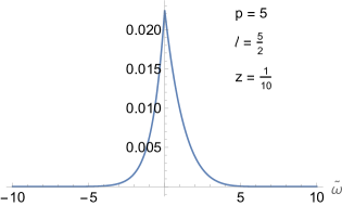
Figure 4: Typical integrand in (108) as a function of the shifted frequency ${\widetilde{\omega}}$ (48). We have fixed the space-time parameters to be $M=10$, $L=1$, $a=1/2$ and the scalar field effective mass (33) to be $\nu=1/100$. The integrand is shown for radial coordinate $z=1/10$ (55), for the scalar field mode with $p=5$ and $\ell=5/2$.

The integrand in (108) has the following key features. First, for $p\neq 0$ it is not symmetric about ${\widetilde{\omega}}=0$. We therefore compute the integral over the whole range of positive and negative ${\widetilde{\omega}}$. The radial function $X_{\omega p\ell}(r)$ (and hence the integrand in (108)) is unchanged under the transformation $\omega\rightarrow-\omega$, $p\rightarrow-p$ (from (43)), and hence the integrand is invariant if we take $p\rightarrow-p$ as well as ${\widetilde{\omega}}\rightarrow-{\widetilde{\omega}}$. This means that it is sufficient to compute the integrals for $p\geq 0$. Second, the integrand is regular for all ${\widetilde{\omega}}$. At ${\widetilde{\omega}}=0$, the double zero in the denominator of the integrand does not lead to a divergence, as $|X_{\omega p\ell}(r)|$ is also zero for ${\widetilde{\omega}}=0$. We do however see a cusp in the integrand when ${\widetilde{\omega}}=0$, due to the presence of the absolute value of ${\widetilde{\omega}}$ in the terms in the denominator of the integrand. Third, as expected from the form of the denominator in the integrand in (108), the integrand tends to zero very rapidly for $|{\widetilde{\omega}}|\rightarrow\infty$.

The integrals $I_{p\ell}(r)$ are computed using Mathematica’s built-in NIntegrate function. We use a working precision of 32 figures and integrate over $|{\widetilde{\omega}}|\leq 30$. The relative errors due to truncating the integrals at this value of $|{\widetilde{\omega}}|$ are extremely small, for example, we estimate this error to be less than $10^{-12}$ for the mode shown in Fig. 4. The peak in the integrand typically increases with decreasing $z$, and decreases as either $p$ or $\ell$ increase. While it is convenient from the point of view of coding that the radial functions are given in terms of Heun functions, in practice the integrals $I_{p\ell}(r)$ require significant computation time, due to the numerical evaluation of these Heun functions. The integrals $I_{p\ell}(r)$ are evaluated on an evenly-spaced grid of 99 values of $z\in(0,1)$, for values of $p$ and $\ell$ discussed below.

Once we have the integrals $I_{p\ell}(r)$, it remains to perform the sum over the quantum numbers $p$ and $\ell$. We write (107) as

$$\Delta{\hat{\Phi}}^{2} =\frac{1}{32\pi^{3}}\sum_{p=-\infty}^{\infty}\sum_{\ell=|p|/2}^{\infty}\left(2\ell+1\right)I_{p\ell}(r)$$

$$=\frac{1}{32\pi^{3}}\sum_{2\ell=0}^{\infty}\sum_{p=-2\ell}^{2\ell}\left(2\ell+1\right)I_{p\ell}(r),$$ (109)

where in the second line we have rewritten the two infinite sums over $\ell$ and $p$ in an equivalent form. This leaves us with a sum over a finite range of the quantum number $p$, and only a final sum over an infinite range of values of $\ell$. Recall that $\ell$ is either an integer or a half-integer, therefore we sum over the positive integer values of $2\ell$.

The finite sum over $p$ is readily computed for each value of $\ell$ and $z$. Defining

$$S_{\ell}(r)=\frac{1}{32\pi^{3}}\sum_{p=-2\ell}^{2\ell}\left(2\ell+1\right)I_{p\ell}(r),$$ (110)

the final step in our computation of the vacuum polarization is to evaluate

$$\Delta{\hat{\Phi}}^{2}=\sum_{2\ell=0}^{\infty}S_{\ell}(r).$$ (111)

Typical summands $S_{\ell}(r)$ are shown in Fig. 5 for a selection of values of the radial coordinate $z$ (55) and the same space-time and scalar field parameters as in Fig. 4.

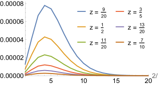
Figure 5: Summand $S_{\ell}(r)$ (110) as a function of $2\ell$ for a selection of values of $z$ (55). The space-time and scalar field parameters are as in Fig. 4.

The profiles of $S_{\ell}$ as a function of $2\ell$ have similar shapes for all values of $z$ in Fig. 5. In particular, there is a peak in the value of $S_{\ell}$ at $\ell\sim 4$ for each value of $z$, and $S_{\ell}$ then decreases rapidly as $\ell$ increases. The value of $S_{\ell}$ at the peak increases as $z$ decreases, and $S_{\ell}$ is significantly greater than zero for larger values of $\ell$ as $z$ decreases.

The partial sums

$${\widetilde{S}}_{\ell}(r)=\sum_{2{{\ell^{\prime}}}=0}^{2\ell}S_{{\ell}^{\prime}}(r)$$ (112)

are shown in Fig. 6 for a selection of values of $z$.

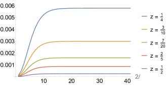
Figure 6: Partial sums ${\widetilde{S}}_{\ell}$ (112) as a function of $2\ell$ for a selection of values of $z$ (55). The space-time and scalar field parameters are as in Fig. 4.

For each value of $z$, the partial sums converge for large $2\ell$, with the limit increasing as $z$ decreases. To check the convergence of the sums over $\ell$, in Fig. 7 we plot the ratio of the summands $S_{\ell+1}/S_{\ell}$ as a function of $2\ell$, again for a selection of values of $z$.

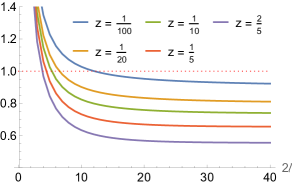
Figure 7: Ratio of the summands $S_{\ell+1}/S_{\ell}$ (110) as a function of $2\ell$ for a selection of values of $z$ (55). The space-time and scalar field parameters are as in Fig. 4.

We find that the ratio is less than unity for $2\ell$ sufficiently large, demonstrating the convergence of the sums. However, the sums over $2\ell$ are not uniformly convergent as $z$ varies, with the rate of convergence decreasing as $z$ decreases. We also check our final answers for the sum (111) obtained by direct summation with those obtained using sequence acceleration methods such as the Shanks transformation [85, 86, 7] (see also [87] for a review of sequence acceleration methods). We truncate the sum (111) at $2\ell=40$, which gives small relative errors, for example, at $z=\frac{1}{2}$ we estimate the error to be of the order of $10^{-8}$.

V.1.2 Numerical results

We are now in a position to present, in Fig. 8, our results for the vacuum polarization (105).

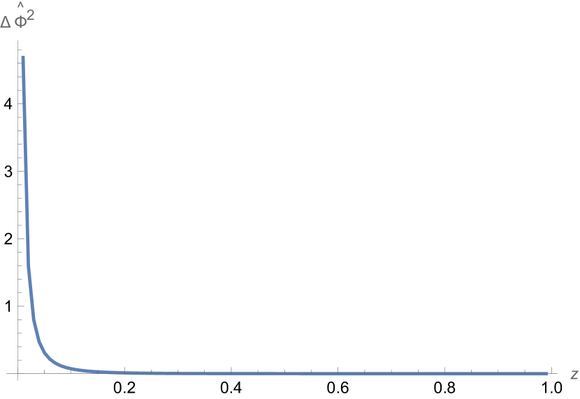
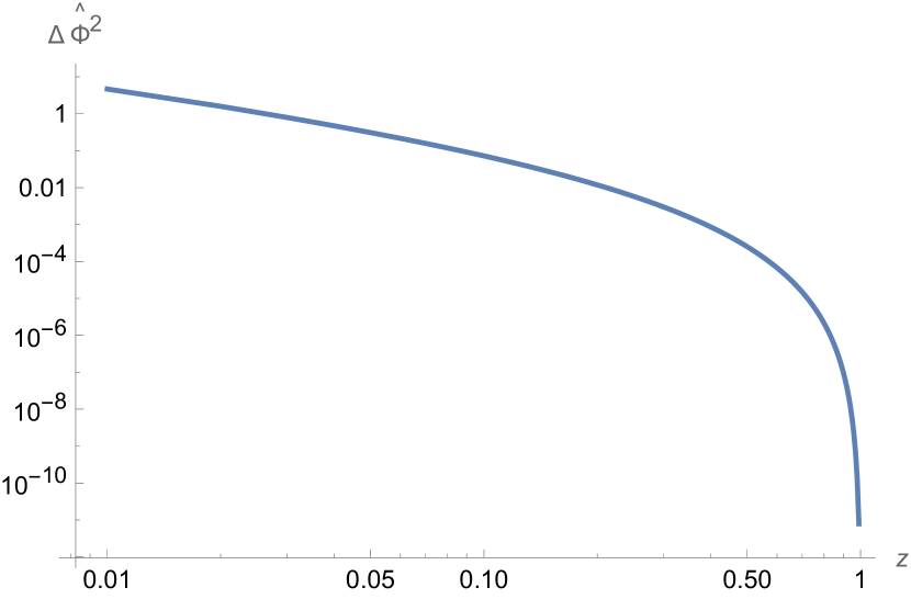
Figure 8: Difference in expectation values of the vacuum polarization in the Hartle-Hawking and Boulware states (105) as a function of the radial coordinate $z$ (55), using a linear scale (upper plot) or a log-log scale (lower plot). The space-time and scalar field parameters are as in Fig. 4.

We fix the space-time parameters to be $M=10$, $L=1$ and $a=1/2$, with a scalar field effective mass (33) of $\nu=1/100$. The upper plot in Fig. 8 shows the difference in the vacuum polarization between the Hartle-Hawking and Boulware states, using a linear scale. It can be seen that this difference tends to zero as $z\rightarrow 1$ (and we approach the anti-de Sitter boundary at $r\rightarrow\infty)$ but diverges as $z\rightarrow 0$ (and we approach the event horizon). In the upper plot in Fig. 8, the difference in vacuum polarization is indistinguishable from zero for $z\gtrsim 0.2$. Therefore, in the lower plot in Fig. 8, we show the same results but on a log-log scale, which makes the range of scales involved clearer.

The Boulware state $|{\mathrm{B}}\rangle$ is expected to be a vacuum state far from the black hole, that is, to be as empty of particles as possible. We would therefore expect that $\langle{\rm{B}}|{\hat{\Phi}}^{2}|{\rm{B}}\rangle$ tends to zero as $r\rightarrow\infty$ and $z\rightarrow 1$. If this is the case, then the results in Fig. 8 imply that $\langle{\rm{H}}|{\hat{\Phi}}^{2}|{\rm{H}}\rangle$ also tends to zero as $z\rightarrow 1$. The Hartle-Hawking state $|{\rm{H}}\rangle$ represents a black hole in thermal equilibrium with a heat bath at the Hawking temperature $\kappa_{+}/2\pi$. The vacuum polarization for a quantum scalar field in a thermal equilibrium state in pure anti-de Sitter space-time tends to its vacuum expectation value at the boundary [88, 89, 90, 91, 92]. We would therefore expect that the vacuum polarization in the Hartle-Hawking state (a thermal state) approaches that in the Boulware state (a vacuum state) far from the black hole.

At the event horizon, we anticipate that the Hartle-Hawking state $|{\rm{H}}\rangle$ is regular, in which case our results imply that the vacuum polarization in the Boulware state $|{\rm{B}}\rangle$ is divergent. This is in agreement with the divergence of $\langle{\rm{B}}|{\hat{\Phi}}^{2}|{\rm{B}}\rangle$ at the event horizon of, for example, a Schwarzschild black hole [44, 93].

On pure AdS space-time, the properties of the vacuum polarization (and, indeed, the SET tensor, as will be discussed in Sec. V.2) for a thermal state, as well as being affected by the boundary conditions applied to the scalar field [90, 91, 92], are a result of the fact that the local temperature $\beta^{-1}$ (where $\beta$ is the inverse temperature) is not a constant in a curved space-time [94, 95]. The role this nonconstant local temperature plays can be investigated by modelling the quantum scalar field as a gas of relativistic particles, using relativistic kinetic theory (RKT) [96]. On AdS, quantum corrections to the RKT results for nonrotating thermal states are small for massless, conformally coupled fields at high temperature [97, 98, 89], and in other regimes (for nonconformally coupled fields, and at lower temperatures), RKT values display qualitatively similar behaviour to the quantum expectation values. In particular, the local temperature in AdS has a maximum value at the origin and tends to zero on the space-time boundary [89], as is the case for the difference in the vacuum polarization between a thermal and vacuum state, at least for a massless conformally or minimally coupled scalar field with Dirichlet boundary conditions applied [89] (see [90, 91, 92] for the corresponding results for different boundary conditions and couplings).

In App. B we use RKT to find the energy density $E_{{\textrm{\tiny{RKT}}}}$ and pressure $P_{{\textrm{\tiny{RKT}}}}$ for a thermal gas of particles of mass $\mu_{{\textrm{\tiny{RKT}}}}$ on the background space-time with metric (1). We take the local inverse temperature in this case to be (154)

$$\beta_{{\textrm{\tiny{RKT}}}}=\frac{2\pi}{\kappa_{+}}{\sqrt{f(r)^{2}-h(r)^{2}\left[\Omega(r)-\Omega_{+}\right]^{2}}},$$ (113)

where $\kappa_{+}$ (19) is the surface gravity of the event horizon, and $\Omega_{+}$ (18) is its angular speed (the metric functions can be found in (1b–1e)). The inverse temperature (113) is the local inverse temperature for an observer at constant $(r,\theta,\varphi)$, rigidly-rotating with the angular speed $\Omega_{+}$ (18) of the event horizon. Using the metric functions (1b–1e), we find, as in pure AdS, that the inverse temperature $\beta_{{\textrm{\tiny{RKT}}}}$ (113) diverges as $r\rightarrow\infty$ and hence the local temperature vanishes on the space-time boundary. Near the event horizon at $r=r_{+}$, since $f(r_{+})=0$ and $\Omega(r_{+})=\Omega_{+}$, the local inverse temperature (113) tends to zero, which means that the local temperature diverges. This does not contradict the expected regularity of the Hartle-Hawking state $|{\rm{H}}\rangle$ (a thermal state) at the event horizon. The observer relative to which the local inverse temperature (113) is defined is an accelerating observer (since they are at constant $r$), and their proper acceleration will diverge as $r\rightarrow r_{+}$. It is therefore unsurprising that the local temperature $\beta_{{\textrm{\tiny{RKT}}}}^{-1}$ for this observer also diverges as $r\rightarrow r_{+}$. In contrast, the Hartle-Hawking state corresponds to a ground state as seen by a freely-falling observer close to the event horizon, and hence is expected to be regular as $r\rightarrow r_{+}$.

We now use $E_{{\textrm{\tiny{RKT}}}}$ and $P_{{\textrm{\tiny{RKT}}}}$ to give an RKT approximation to the difference in vacuum polarization between a thermal and vacuum state (see, for example, [98, 99] for the corresponding quantity for fermion fields on pure AdS):

$$\Delta\Phi^{2}_{{\textrm{\tiny{RKT}}}}=\frac{1}{\mu_{{\textrm{\tiny{RKT}}}}}\left(E_{{\textrm{\tiny{RKT}}}}-4P_{{\textrm{\tiny{RKT}}}}\right)\\ =\frac{\mu_{{\textrm{\tiny{RKT}}}}}{4\pi^{2}\beta_{{\textrm{\tiny{RKT}}}}^{3}}\left[\left(\beta_{{\textrm{\tiny{RKT}}}}\mu_{{\textrm{\tiny{RKT}}}}\right)\,{\mathrm{Li}}_{2}({\mathsf{Y}})+{\mathrm{Li}}_{3}({\mathsf{Y}})\right],$$ (114)

where ${\mathrm{Li}}_{n}$ is a polylogarithm and ${\mathsf{Y}}=\exp\left(-\beta_{{\textrm{\tiny{RKT}}}}\mu_{{\textrm{\tiny{RKT}}}}\right)$ (164c). We wish to compare the RKT result (114) with the difference in quantum expectation values (105). The latter (the vacuum polarization) depends on the scalar field mass $\mu$ and coupling $\xi$ to the scalar curvature only in the combination $\nu$ (33), which we dub the “scalar field effective mass”. In contrast, the RKT result (114) depends only on the mass $\mu_{{\textrm{\tiny{RKT}}}}$ of the thermal gas of particles. Therefore there is some degeneracy in the possible choices of $\mu_{{\textrm{\tiny{RKT}}}}$ for fixed $\nu$. In Fig. 9 we compare our numerical results for the quantum difference in vacuum polarization $\Delta{\hat{\Phi}}^{2}$ (105) with the prediction from RKT (114). We make two natural choices of the coupling constant $\xi$: firstly minimal coupling $\xi=0$ (in which case $\mu_{{\textrm{\tiny{RKT}}}}=\nu$), and secondly conformal coupling $\xi=3/16$ (in which case $\mu_{{\textrm{\tiny{RKT}}}}^{2}L^{2}=\nu^{2}L^{2}+15/4$). Note that the RKT particle mass $\mu_{{\textrm{\tiny{RKT}}}}$ is larger for conformal coupling than for minimal coupling.

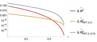
Figure 9: Comparison between the RKT approximation $\Delta\Phi^{2}_{{\textrm{\tiny{RKT}}}}$ (114) to the vacuum polarization for both minimal ($\xi=0$) and conformal ($\xi=3/16$) coupling and the difference $\Delta{\hat{\Phi}}^{2}$ (105) in vacuum polarization between the Hartle-Hawking and Boulware states. The space-time and scalar field parameters are as in Fig. 4.

We can see from Fig. 9 that the RKT expression (114) does not approximate the quantum vacuum polarization particularly well for either value of the coupling constant $\xi$; we conclude that quantum effects are significant. However, the RKT approximation does share some qualitative features with the vacuum polarization: it diverges at the event horizon (due to the divergence of the local temperature $\beta_{{\textrm{\tiny{RKT}}}}^{-1}$ (113)) and vanishes as the space-time boundary is approached (since the local temperature also vanishes on the boundary). Near the event horizon, using the results (167), the RKT approximation (114) is proportional to $\mu_{{\textrm{\tiny{RKT}}}}\beta_{{\textrm{\tiny{RKT}}}}^{-3}$. This is in accordance with Fig. 9, where the curves corresponding to the RKT approximation (114) for $\xi=0$ and $\xi=3/16$ have similar slopes for small $z$, with the latter curve taking larger values than the former. For small $z$, the difference in the vacuum polarization between the Hartle-Hawking and Boulware states takes values between the two RKT approximations with $\xi=0$ and $\xi=3/16$, but the VP appears to be diverging more quickly as the horizon is approached. At infinity, again using the results (167), we see that the RKT approximation (114) is proportional to $\mu_{{\textrm{\tiny{RKT}}}}^{2}\beta_{{\textrm{\tiny{RKT}}}}^{-2}\exp\left(-\beta_{{\textrm{\tiny{RKT}}}}\mu_{{\textrm{\tiny{RKT}}}}\right)$. This can be seen in Fig. 9; the approximation with $\xi=3/16$ (for which the mass $\mu_{{\textrm{\tiny{RKT}}}}$ is larger) takes larger values for most of the range of $z$ considered, but is vanishing more rapidly as $z$ increases. For larger $z$, the difference in the vacuum polarization is smaller than either of the RKT approximations, and also seems to be tending to zero more quickly.

V.2 Stress-energy tensor

We now turn to the expectation value of the quantum SET operator ${\hat{T}}_{\mu\nu}$. Analogously to the vacuum polarization (105), we find

$$\Delta{\hat{T}}_{\mu\nu}=\langle{\rm{H}}|{\hat{T}}_{\mu\nu}|{\rm{H}}\rangle-\langle{\rm{B}}|{\hat{T}}_{\mu\nu}|{\rm{B}}\rangle\\ =\sum_{p=-\infty}^{\infty}\sum_{\ell=|p|/2}^{\infty}\sum_{m=-\ell}^{\ell}\int_{{\widetilde{\omega}}=-\infty}^{\infty}d{\widetilde{\omega}}\\ \times\frac{{}^{\aleph}T_{\mu\nu}}{\exp\left(2\pi{\widetilde{\omega}}/{\kappa_{+}}\right)-1},$$ (115)

where ${}^{\aleph}T_{\mu\nu}$ is the classical SET for a scalar field mode (35) and we use the notation $\aleph=\{\omega,p,\ell,m\}$ to denote the quantum numbers on which this mode contribution to the SET depends. In five space-time dimensions, there are fifteen independent components of the SET, since it is a symmetric tensor. Using the mode solutions (35) of the scalar field equation, the form of these components ${}^{\aleph}T_{\mu\nu}$ can be derived in terms of the radial and angular functions $X_{\omega p\ell}(r)$ (65) and ${}_{s}{\widetilde{Y}}_{\ell}^{m}(\theta)$ (37). The resulting expressions are rather lengthy, so are presented in App. C.

In this section, before we proceed to the numerical computation of $\Delta{\hat{T}}_{\mu\nu}$ (115) and a discussion of our numerical results, we first simplify the components of $\Delta{\hat{T}}_{\mu\nu}$ using the general principles of conservation and the underlying symmetries of the background space-time (1).

V.2.1 General properties of the stress-energy tensor

In this subsection, we use the symmetries of the space-time (1) to constrain the form of the SET (115), assuming that this shares these symmetries of the underlying black hole geometry.

In particular, we assume that the SET preserves the space-time symmetries resulting from the Killing vectors (7), so that the Lie derivatives of the SET along each of these Killing vectors vanish:

$${\mathcal{L}}_{{\mathcal{V}}_{i}}\langle{\hat{T}}^{\mu\nu}\rangle=0,\qquad i=0,1,\ldots,5.$$ (116)

Applying this to the first three Killing vectors (7a), we conclude that the components of $\langle{\hat{T}}^{\mu\nu}\rangle$ are independent of the coordinates $t$, $\varphi$ and $\psi$. The remaining independent Killing vectors, ${\mathcal{V}}_{4}$ (7b) and ${\mathcal{V}}_{5}$ (7c), give more complicated constraints. Writing the Lie derivative ${\mathcal{L}}_{{\mathcal{V}}_{i}}\langle{\hat{T}}_{\mu\nu}\rangle$ as

$$0= ~{}{\mathcal{L}}_{{\mathcal{V}}_{i}}\langle{\hat{T}}_{\mu\nu}\rangle$$

$$= ~{}{\mathcal{V}}_{i}^{\alpha}\partial_{\alpha}\langle{\hat{T}}^{\mu\nu}\rangle-\left(\partial_{\alpha}{\mathcal{V}}_{i}^{\mu}\right)\langle{\hat{T}}^{\alpha\nu}\rangle-\left(\partial_{\alpha}{\mathcal{V}}_{i}^{\nu}\right)\langle{\hat{T}}^{\mu\alpha}\rangle,$$ (117)

gives fifteen equations for each of the two remaining Killing vectors. Considering the combination ${\mathcal{L}}_{{\mathcal{V}}_{4}}\langle{\hat{T}}^{\mu\nu}\rangle\sin\varphi+{\mathcal{L}}_{{\mathcal{V}}_{5}}\langle{\hat{T}}^{\mu\nu}\rangle\cos\varphi$ immediately gives that the following SET components vanish identically:

$$\langle{\hat{T}}^{t\theta}\rangle=\langle{\hat{T}}^{t\varphi}\rangle=\langle{\hat{T}}^{r\theta}\rangle=\langle{\hat{T}}^{r\varphi}\rangle=\langle{\hat{T}}^{\theta\varphi}\rangle=\langle{\hat{T}}^{\theta\psi}\rangle=0,$$ (118)

as well as the following relations:

$$\langle{\hat{T}}^{\varphi\varphi}\rangle =\frac{\langle{\hat{T}}^{\theta\theta}\rangle}{\sin^{2}\theta},$$ (119a)

$$\langle{\hat{T}}^{\varphi\psi}\rangle =-\frac{\langle{\hat{T}}^{\theta\theta}\rangle}{2\tan\theta\sin\theta}.$$ (119b)

Next we consider ${\mathcal{L}}_{{\mathcal{V}}_{4}}\langle{\hat{T}}^{\mu\nu}\rangle\cos\varphi-{\mathcal{L}}_{{\mathcal{V}}_{5}}\langle{\hat{T}}^{\mu\nu}\rangle\sin\varphi$, from which we deduce that the following components of the SET do not depend on the angle $\theta$: $\langle{\hat{T}}^{tt}\rangle$, $\langle{\hat{T}}^{tr}\rangle$, $\langle{\hat{T}}^{t\psi}\rangle$, $\langle{\hat{T}}^{rr}\rangle$, $\langle{\hat{T}}^{r\psi}\rangle$ and $\langle{\hat{T}}^{\theta\theta}\rangle$. There is one further relation arising from this combination of Lie derivatives, which takes the form

$$\partial_{\theta}\langle{\hat{T}}^{\psi\psi}\rangle=-\frac{\langle{\hat{T}}^{\theta\theta}\rangle}{2\tan\theta\sin^{2}\theta},$$ (120a)

and which is readily integrated to give

$$\langle{\hat{T}}^{\psi\psi}\rangle=\frac{\langle{\hat{T}}^{\theta\theta}\rangle}{4\sin^{2}\theta}+{\mathcal{F}}^{\psi\psi}(r),$$ (120b)

where ${\mathcal{F}}^{\psi\psi}(r)$ is an arbitrary function of $r$. In summary, we can write the SET in matrix form as follows:

$$\langle{\hat{T}}^{\mu\nu}\rangle=\left(\begin{array}[]{ccccc}{\mathcal{F}}^{tt}(r)&{\mathcal{F}}^{tr}(r)&0&0&{\mathcal{F}}^{t\psi}(r)\\ {\mathcal{F}}^{tr}(r)&{\mathcal{F}}^{rr}(r)&0&0&{\mathcal{F}}^{r\psi}(r)\\ 0&0&{\mathcal{F}}^{\theta\theta}(r)&0&0\\ 0&0&0&\dfrac{{\mathcal{F}}^{\theta\theta}(r)}{\sin^{2}\theta}&-\dfrac{{\mathcal{F}}^{\theta\theta}(r)}{2\tan\theta\sin\theta}\\[8.5359pt] {\mathcal{F}}^{t\psi}(r)&{\mathcal{F}}^{r\psi}(r)&0&-\dfrac{{\mathcal{F}}^{\theta\theta}(r)}{2\tan\theta\sin\theta}&\dfrac{{\mathcal{F}}^{\theta\theta}(r)}{4\sin^{2}\theta}+{\mathcal{F}}^{\psi\psi}(r)\end{array}\right),$$ (121)

where the ${\mathcal{F}}^{\bullet\bullet}(r)$ are arbitrary functions of $r$. We note that the underlying symmetries of the black hole geometry have completely fixed the dependence of the SET components on the angle $\theta$ (as is the case for static, spherically symmetric black holes), and we are left with seven arbitrary functions of $r$ which are to be determined.

We can further constrain these seven arbitrary functions of $r$ by imposing the requirement that the SET is conserved:

$$\nabla_{\nu}\langle{\hat{T}}_{\mu}{}^{\nu}\rangle=0,$$ (122)

which we write in the alternative form

$$\partial_{\nu}\left({\mathsf{g}}\langle{\hat{T}}_{\mu}{}^{\nu}\rangle\right)=\frac{1}{2}{\mathsf{g}}\left(\partial_{\mu}g_{\alpha\beta}\right)\langle{\hat{T}}^{\alpha\beta}\rangle,$$ (123)

where ${\mathsf{g}}$ is given by (3). Comparing the form of the metric (1) and the SET (121), we have immediately that the $\mu=\theta$ equation is trivial. Since the metric (1) does not depend on $t$, $\varphi$ or $\psi$, there are three simple conservation equations arising from (123). The $\varphi$ and $\psi$ equations are identical, and give

$$\frac{d}{dr}{\mathcal{F}}_{1}(r)+\left[\frac{2}{r}+\frac{f^{\prime}(r)}{f(r)}+\frac{g^{\prime}(r)}{g(r)}+3\frac{h^{\prime}(r)}{h(r)}\right]{\mathcal{F}}_{1}(r)=0,$$ (124a)

where we have defined

$${\mathcal{F}}_{1}(r)={\mathcal{F}}^{r\psi}(r)-\Omega(r){\mathcal{F}}^{tr}(r)$$ (124b)

and $f(r)$, $g(r)$, $h(r)$ and $\Omega(r)$ are the metric functions given in (1b–1e). Integrating (124) yields

$${\mathcal{F}}_{1}(r)=\frac{{\mathcal{Y}}}{r^{2}f(r)g(r)h(r)^{3}}=\frac{{\mathcal{Y}}}{r^{3}h(r)^{2}},$$ (125)

where ${\mathcal{Y}}$ is an arbitrary constant. The $\mu=t$ equation arising from (123) then takes the form

$$\frac{d}{dr}{\mathcal{F}}^{tr}(r)+\left(\frac{2}{r}+\frac{3f^{\prime}(r)}{f(r)}+\frac{g^{\prime}(r)}{g(r)}+\frac{h^{\prime}(r)}{h(r)}\right){\mathcal{F}}^{tr}(r)\\ +\frac{{\mathcal{Y}}\Omega^{\prime}(r)}{r^{3}f(r)^{2}}=0.$$ (126)

This is also readily integrated to give

$${\mathcal{F}}^{tr}(r)=\frac{{\mathcal{Z}}-{\mathcal{Y}}\Omega(r)}{r^{2}f(r)^{3}g(r)h(r)}=\frac{{\mathcal{Z}}-{\mathcal{Y}}\Omega(r)}{r^{3}f(r)^{2}},$$ (127)

where ${\mathcal{Z}}$ is an arbitrary constant. Hence, using (124b), we have

$${\mathcal{F}}^{r\psi}(r)=\frac{1}{r^{3}f(r)^{2}h(r)^{2}}\\ \times\left({\mathcal{Y}}f(r)^{2}+h(r)^{2}\Omega(r)\left[{\mathcal{Z}}-{\mathcal{Y}}\Omega(r)\right]\right).$$ (128)

The remaining conservation equation (123) has $\mu=r$ and is more complicated:

$$0= ~{}\frac{d}{dr}{\mathcal{F}}^{rr}(r)+\left[\frac{2}{r}+\frac{f^{\prime}(r)}{f(r)}+\frac{2g^{\prime}(r)}{g(r)}+\frac{h^{\prime}(r)}{h(r)}\right]{\mathcal{F}}^{rr}(r)-\frac{1}{4g(r)^{2}}\left[2r+h(r)h^{\prime}(r)\right]{\mathcal{F}}^{\theta\theta}(r)$$

$$~{}+\frac{1}{g(r)^{2}}\left\{\left[f(r)f^{\prime}(r)-h(r)h^{\prime}(r)\Omega(r)^{2}-h(r)^{2}\Omega(r)\Omega^{\prime}(r)\right]{\mathcal{F}}^{tt}(r)+\left[2h(r)h^{\prime}(r)\Omega(r)+h(r)^{2}\Omega^{\prime}(r)\right]{\mathcal{F}}^{t\psi}(r)\right.$$

$$~{}\left.-h(r)h^{\prime}(r){\mathcal{F}}^{\psi\psi}(r)\right\}.$$ (129)

Nonetheless, (129) can be integrated directly to give ${\mathcal{F}}^{rr}(r)$:

$${\mathcal{F}}^{rr}(r)=\frac{1}{r^{3}g(r)}\left[{\mathcal{K}}+\int_{r^{\prime}=r_{+}}^{r}\Theta(r^{\prime})\,dr^{\prime}\right],$$ (130)

where ${\mathcal{K}}$ is an arbitrary constant and we have defined

$$\Theta(r)=\frac{r^{3}}{g(r)}\bigg{\{}\left[f(r)f^{\prime}(r)-h(r)h^{\prime}(r)\Omega(r)^{2}-h(r)^{2}\Omega(r)\Omega^{\prime}(r)\right]{\mathcal{F}}^{tt}(r)+\left[2h(r)h^{\prime}(r)\Omega(r)+h(r)^{2}\Omega^{\prime}(r)\right]{\mathcal{F}}^{t\psi}(r)\\ -h(r)h^{\prime}(r){\mathcal{F}}^{\psi\psi}(r)-\frac{1}{4}\left[2r+h(r)h^{\prime}(r)\right]{\mathcal{F}}^{\theta\theta}(r)\bigg{\}}.$$ (131)

In summary, using the symmetries of the underlying space-time and the conservation of the SET, we have found that the SET is determined by three arbitrary constants (${\mathcal{K}}$, ${\mathcal{Y}}$ and ${\mathcal{Z}}$) and four arbitrary functions of the radial coordinate $r$ only, namely ${\mathcal{F}}^{\theta\theta}(r)$, ${\mathcal{F}}^{tt}(r)$, ${\mathcal{F}}^{t\psi}(r)$ and ${\mathcal{F}}^{\psi\psi}(r)$. The enhanced symmetry of the space-time compared to the four-dimensional Kerr metric has played a significant role here, enabling us to constrain the SET much more than in the Kerr case [24]. For Kerr, using the Killing vectors and the conservation equations gives the four-dimensional SET in terms of two arbitrary functions of the latitudinal angle $\theta$ and six functions of both $\theta$ and $r$, which are constrained by two coupled equations [24]. In our situation, the enhanced symmetry has completely determined the angular dependence of the SET, as well as reducing the number of unknown components. At the same time, the SET structure in our scenario is more complicated than that on a five-dimensional static, spherically symmetric space-time [100], which is determined by just two arbitrary constants and two arbitrary functions of the radial coordinate.

There is one further constraint on the SET components, namely the trace $\langle{\hat{T}}_{\mu}^{\mu}\rangle$. For a massless, conformally-coupled scalar field, this is given by the trace anomaly, which vanishes in five space-time dimensions [58]. When the scalar field has general mass $\mu$ and coupling $\xi$ to the scalar curvature, the trace $\langle{\hat{T}}_{\mu}^{\mu}\rangle$ is given by [58]

$$\langle{\hat{T}}_{\mu}^{\mu}\rangle=-\mu^{2}\langle{\hat{\Phi}}^{2}\rangle+4\left(\xi-\frac{3}{16}\right)\Box\langle{\hat{\Phi}}^{2}\rangle,$$ (132)

which depends on the vacuum polarization $\langle{\hat{\Phi}}^{2}\rangle$ and its derivatives and clearly vanishes when the field is massless ($\mu=0$) and conformally coupled ($\xi=3/16$). Since the vacuum polarization is not known a priori and can only be computed numerically, (132) does not reduce the number of unknown functions, but it does provide a useful check of our numerical results. In particular, using the SET form (121) and metric (1), we have

$$\langle{\hat{T}}_{\mu}^{\mu}\rangle= \left[-f(r)^{2}+h(r)^{2}\Omega(r)^{2}\right]{\mathcal{F}}^{tt}(r)$$

$$-2h(r)^{2}\Omega(r){\mathcal{F}}^{t\psi}(r)+g(r)^{2}{\mathcal{F}}^{rr}(r)$$

$$+\frac{1}{4}\left[2r^{2}-h(r)^{2}\right]{\mathcal{F}}^{\theta\theta}(r)+h(r)^{2}{\mathcal{F}}^{\psi\psi}(r).$$ (133)

At least in principle, we could use (133) to eliminate say ${\mathcal{F}}^{\psi\psi}(r)$ from (129) and then integrate to give an alternative expression for ${\mathcal{F}}^{rr}(r)$, which would involve the trace $\langle{\hat{T}}_{\mu}^{\mu}\rangle$. However, there is no great advantage in doing so, and we shall instead use (133) as a check of our numerical results, which are discussed in the next subsection.

V.2.2 Numerical method

To find the difference in expectation values of the SET between the Hartle-Hawking and Boulware states, $\Delta{\hat{T}}_{\mu\nu}$ (115), from the analysis of the previous subsection we require the determination of three arbitrary constants (${\mathcal{K}}$, ${\mathcal{X}}$ and ${\mathcal{Z}}$) and the numerical computation of four functions of the radial coordinate $r$ (${\mathcal{F}}^{\theta\theta}(r)$, ${\mathcal{F}}^{tt}(r)$, ${\mathcal{F}}^{t\psi}(r)$, and ${\mathcal{F}}^{\psi\psi}(r)$, where the functions ${\mathcal{F}}^{\bullet\bullet}(r)$ now refer to those pertinent to this difference in SET expectation values).

Our overall strategy for the numerical computation of the functions ${\mathcal{F}}^{\bullet\bullet}(r)$ and hence the SET components (115) follows that for the vacuum polarization in Sec. V.1.1. First we require mode sum expressions for the functions ${\mathcal{F}}^{\bullet\bullet}(r)$. To find these, we start with the expressions for ${}^{\aleph}T_{\mu\nu}$, the classical SET components for a scalar field mode (35), which are given in (173). Next we perform the sum over the quantum number $m$, using the addition theorems for spin-weighted spherical harmonics in App. A. The resulting quantities can be found in (175). From these, we can write each ${\mathcal{F}}^{\bullet\bullet}(r)$ as a mode sum over the shifted frequency ${\widetilde{\omega}}$ and quantum numbers $p$ and $\ell$:

$${\mathcal{F}}^{\bullet\bullet}(r)=\frac{1}{4\pi}\sum_{2\ell=0}^{\infty}\sum_{p=-2\ell}^{2\ell}\int_{{\widetilde{\omega}}=-\infty}^{\infty}d{\widetilde{\omega}}\,\frac{\left(2\ell+1\right){\mathfrak{F}}^{\bullet\bullet}(r)}{\exp\left(2\pi|{\widetilde{\omega}}|/{\kappa_{+}}\right)-1},$$ (134)

where expressions for the individual ${\mathfrak{F}}^{\bullet\bullet}(r)$ can be found in (177). In (134), following (109), we have rewritten the sums over $p=-\infty,\ldots,\infty$ and $2\ell=|p|,\ldots\infty$ as a sum over a finite number of values of $p$ and a sum over $2\ell=0,\ldots\infty$.

From (177), we see that ${\mathfrak{F}}^{tr}(r)=0={\mathfrak{F}}^{r\psi}(r)$ and hence ${\mathcal{F}}^{tr}(r)=0={\mathcal{F}}^{r\psi}(r)$. Hence, using (125, 127), we can immediately fix two of our constants: ${\mathcal{Y}}=0={\mathcal{Z}}$. Instead of finding the constant ${\mathcal{K}}$ and then ${\mathcal{F}}^{rr}(r)$ using (130), we found it more straightforward to calculate ${\mathcal{F}}^{rr}(r)$ directly. This means that we will compute five functions of $r$, namely ${\mathcal{F}}^{\theta\theta}(r)$, ${\mathcal{F}}^{tt}(r)$, ${\mathcal{F}}^{t\psi}(r)$, ${\mathcal{F}}^{\psi\psi}(r)$ and ${\mathcal{F}}^{rr}(r)$.

As in Sec.V.1.1, we first perform the integral over the shifted frequency ${\widetilde{\omega}}$ in (134). Examination of the expressions in (177) reveal that, for each $p$ and $\ell$, we require the following integrals:

$$I^{(1)}_{p\ell}(r) =\int_{{\widetilde{\omega}}=-\infty}^{\infty}d{\widetilde{\omega}}\,\frac{\omega\left|X_{\omega p\ell}(r)\right|^{2}}{|{\widetilde{\omega}}|\left[\exp\left(2\pi|{\widetilde{\omega}}|/{\kappa_{+}}\right)-1\right]},$$ (135a)

$$I^{(2)}_{p\ell}(r) =\int_{{\widetilde{\omega}}=-\infty}^{\infty}d{\widetilde{\omega}}\,\frac{\omega^{2}\left|X_{\omega p\ell}(r)\right|^{2}}{|{\widetilde{\omega}}|\left[\exp\left(2\pi|{\widetilde{\omega}}|/{\kappa_{+}}\right)-1\right]},$$ (135b)

$$I^{(3)}_{p\ell}(r) =\int_{{\widetilde{\omega}}=-\infty}^{\infty}d{\widetilde{\omega}}\,\frac{\Re\{X_{p\ell}^{*}(r)X^{\prime}_{p\ell}(r)\}}{|{\widetilde{\omega}}|\left[\exp\left(2\pi|{\widetilde{\omega}}|/{\kappa_{+}}\right)-1\right]},$$ (135c)

$$I^{(4)}_{p\ell}(r) =\int_{{\widetilde{\omega}}=-\infty}^{\infty}d{\widetilde{\omega}}\,\frac{\left|X_{\omega p\ell}^{\prime}(r)\right|^{2}}{|{\widetilde{\omega}}|\left[\exp\left(2\pi|{\widetilde{\omega}}|/{\kappa_{+}}\right)-1\right]},$$ (135d)

in addition to the integral $I_{p\ell}(r)$ (108) which we have already computed for the vacuum polarization. As for the integrand in $I_{p\ell}(r)$ (see Fig. 4), the integrands in (135) are regular and rapidly decaying as $|{\widetilde{\omega}}|\rightarrow\infty$. The integrals (135) are computed in a similar way to $I_{p\ell}(r)$, using Mathematica’s built-in NIntegrate function, although these have a longer computation time than that required for $I_{p\ell}(r)$.

Once we have found the integrals (135), we take appropriate combinations of these, using (177), to give

$${\widetilde{\mathfrak{F}}}^{\bullet\bullet}_{p\ell}(r)=\int_{{\widetilde{\omega}}=-\infty}^{\infty}d{\widetilde{\omega}}\,\frac{{\mathfrak{F}}^{\bullet\bullet}(r)}{\exp\left(2\pi|{\widetilde{\omega}}|/{\kappa_{+}}\right)-1},$$ (136)

in terms of which we have

$${\mathcal{F}}^{\bullet\bullet}(r)=\frac{1}{4\pi}\sum_{2\ell=0}^{\infty}\sum_{p=-2\ell}^{2\ell}\left(2\ell+1\right){\widetilde{\mathfrak{F}}}^{\bullet\bullet}_{p\ell}(r).$$ (137)

The sums over the quantum number $p$ in (137) are then straightforward to compute, leaving just the sum over $2\ell$. As for the vacuum polarization, we find that summing over values of $2\ell$ from 0 to 40 gives results which are sufficiently accurate for our purposes.

We validate our results by computing the trace of $\Delta{\hat{T}}_{\mu\nu}$ (115) using (133) and compare with the result (132) which involves the difference in vacuum polarization between the Hartle-Hawking and Boulware states. For a conformally coupled field with $\xi=3/16$, we find agreement between these two expressions to one part in $10^{12}$. Ideally, one would also check that our functions ${\mathcal{F}}^{\bullet\bullet}(r)$ satisfy the conservation equation (129) (and that (133) holds for values of $\xi$ other than $3/16$). Performing either of these checks requires derivatives of quantities we have computed numerically. These can be found by interpolating our results between the grid points in $z$ and then differentiating the interpolating function. As might be expected, this introduces additional numerical errors. In our situation, these errors are compounded by the fact that both the difference in vacuum polarization $\Delta{\hat{\Phi}}^{2}$ and the functions ${\mathcal{F}}^{\bullet\bullet}(r)$ vary by several orders of magnitude over the range of values of $z$ (see, for example, Fig. 8). Furthermore, different functions ${\mathcal{F}}^{\bullet\bullet}(r)$ have very different orders of magnitude at the same value of $z$. As a result, neither the conservation equation test, nor the trace test (for nonconformally-coupled fields) is particularly robust. However, we do find, at intermediate values of $z$, that the relative error in the evaluation of the conservation equation (129) is several orders of magnitude smaller than the largest magnitude of the ${\mathcal{F}}^{\bullet\bullet}(r)$ functions, which at least lends credence to our numerical results.

V.2.3 Numerical results

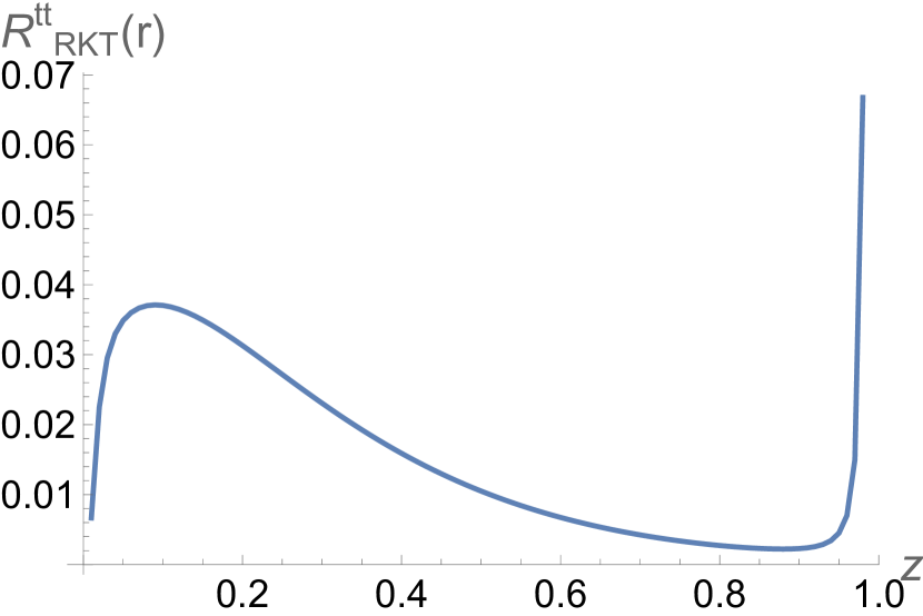
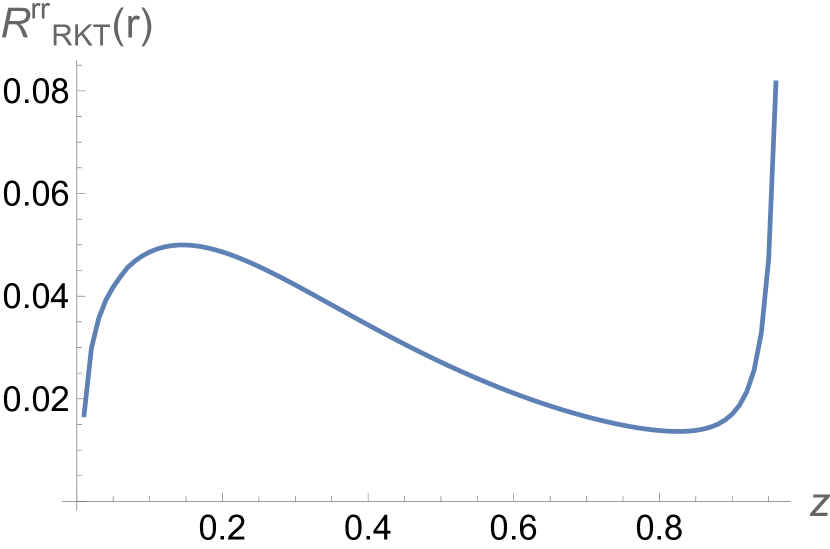
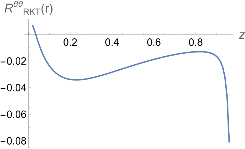
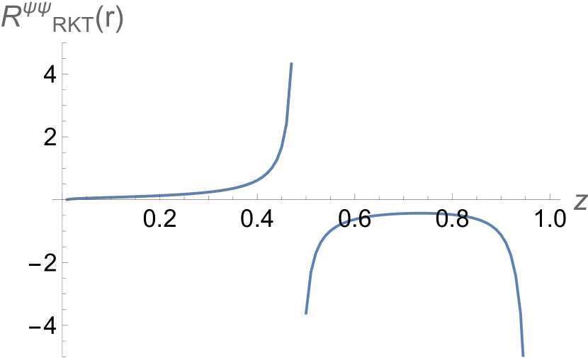
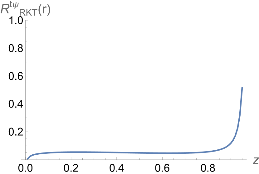
Figure 10: Ratios $R^{\bullet\bullet}_{{\textrm{\tiny{RKT}}}}={\mathcal{F}}^{\bullet\bullet}(r)/{\mathcal{F}}^{\bullet\bullet}_{{\textrm{\tiny{RKT}}}}(r)$ of the functions ${\mathcal{F}}^{\bullet\bullet}(r)$ in the SET (121) with the corresponding functions ${\mathcal{F}}^{\bullet\bullet}_{{\textrm{\tiny{RKT}}}}(r)$ derived using the RKT approximation (170). In both cases the scalar field is assumed to be conformally coupled, $\xi=3/16$. The space-time and scalar field parameters are as in Fig. 4.

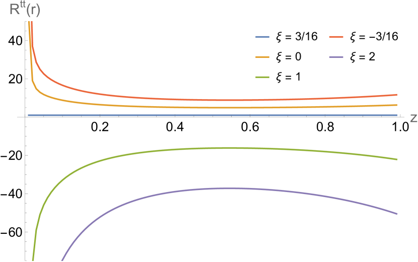
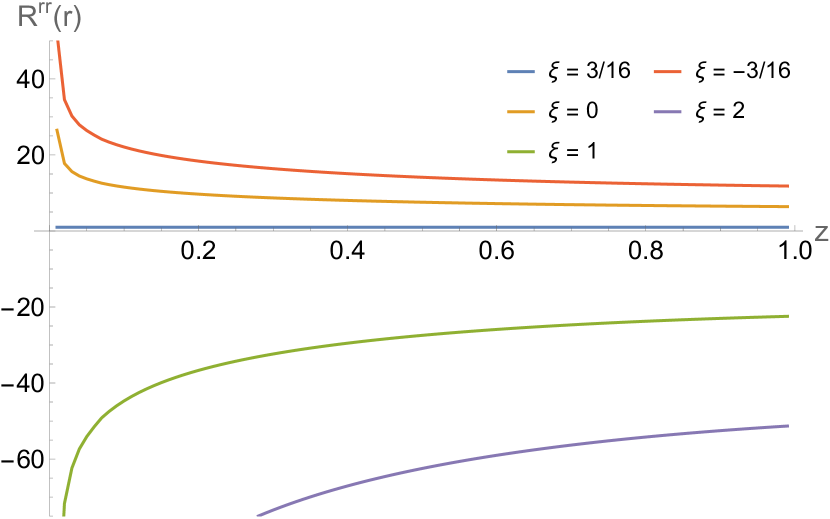
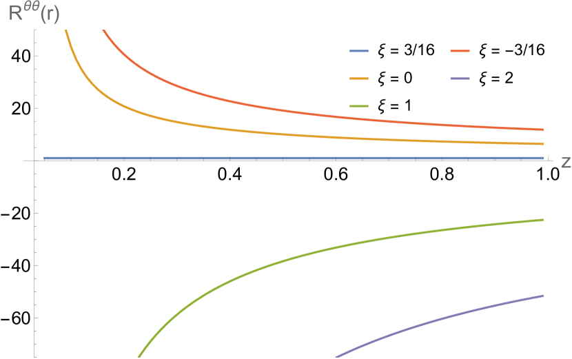
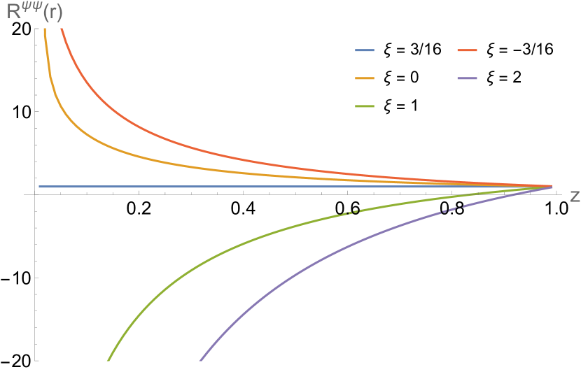
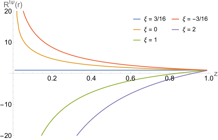
Figure 11: Ratios ${\mathsf{R}}(r)^{\bullet\bullet}={\mathcal{F}}^{\bullet\bullet}(r)/{\mathcal{F}}^{\bullet\bullet}_{\xi=3/16}(r)$ of the functions ${\mathcal{F}}^{\bullet\bullet}(r)$ in the SET (121) for a selection of values of the coupling constant $\xi$ with the corresponding functions when $\xi=3/16$ and the scalar field is conformally coupled. The space-time and scalar field parameters are as in Fig. 4.

If we simply plot the functions ${\mathcal{F}}^{\bullet\bullet}$ as functions of $z$, the resulting graphs are not particularly informative, and are qualitatively very similar to the vacuum polarization shown in Fig. 8. In particular, we find that these functions diverge at the event horizon and rapidly decay to zero as $z\rightarrow 1$. In order to gain more insight into the behaviour of the SET components, we consider instead ratios of the functions ${\mathcal{F}}^{\bullet\bullet}$ with other quantities whose behaviour in these two asymptotic regions is known.

We begin, in Fig. 10, by plotting the ratios $R^{\bullet\bullet}_{{\textrm{\tiny{RKT}}}}(r)={\mathcal{F}}^{\bullet\bullet}(r)/{\mathcal{F}}^{\bullet\bullet}_{{\textrm{\tiny{RKT}}}}(r)$ of the functions ${\mathcal{F}}^{\bullet\bullet}(r)$ in the difference in SET expectation values between the Hartle-Hawking and Boulware states with the corresponding functions ${\mathcal{F}}^{\bullet\bullet}_{{\textrm{\tiny{RKT}}}}(r)$ derived using RKT (the expressions for these can be found in App. B, Eq. (170)). In both cases we consider a conformally coupled scalar field with $\xi=3/16$ and effective mass $\nu=1/100$ (33), using units in which $L=1$. Therefore, in the RKT approximation, we assume that the particles in the gas have mass $\mu_{{\textrm{\tiny{RKT}}}}^{2}=\nu^{2}+15/4$ (again setting $L=1$).

As with the vacuum polarization (see Fig. 9), we see from Fig. 10 that quantum effects are significant. With the notable exception of the ratio $R^{\psi\psi}_{{\textrm{\tiny{RKT}}}}$, these ratios are regular between the event horizon and space-time boundary. The ratio $R^{\psi\psi}_{{\textrm{\tiny{RKT}}}}$ has an asymptote at $z\sim 0.5$. This is due to the RKT expression (170g) vanishing at that value of $z$; the difference in the the quantum expectation values of this component of the SET is finite for all $z\in(0,1)$. Also of note is the fact that the ratio $R^{\theta\theta}_{{\textrm{\tiny{RKT}}}}$ is negative almost everywhere outside the event horizon, so that the function appearing in the difference in expectation values of the quantum SET operator has the opposite sign to that in the RKT approximation.

Near the space-time boundary, all the ratios shown in Fig. 10 are rapidly diverging. This suggests that the RKT quantities are decaying more rapidly to zero than the corresponding quantities in $\Delta{\hat{T}}_{\mu\nu}$. This is in contrast to the vacuum polarization, which appears from Fig. 9 to be decaying more rapidly than the RKT approximation as the boundary is approached.

Close to the event horizon, the ratios are decreasing in magnitude, which implies that the quantum SET quantities are diverging less rapidly than the corresponding RKT quantities. Again, this is in contrast to the vacuum polarization in Fig. 9, which provides evidence that, close to the horizon, the vacuum polarization is diverging more rapidly than the corresponding RKT quantity.

In Sec. V.1.2, we observed that the difference in vacuum polarization between the Hartle-Hawking and Boulware states (105) diverges on the event horizon of the black hole, and attributed this divergence to a divergence in the Boulware state, since we expect the Hartle-Hawking state to be regular at the horizon. To examine whether the same is true for the SET, we need to find its components with respect to the Kruskal coordinates (24), which are regular at the horizon. However, the transformation to Kruskal coordinates does not alter the angular coordinates $(\theta,\varphi)$ and hence we can qualitatively study the divergence of the SET at the horizon by considering the components $\Delta{\hat{T}}_{\theta\theta}$, $\Delta{\hat{T}}_{\varphi\varphi}$, or, equivalently, the function ${\mathcal{F}}^{\theta\theta}(r)$ (121). From the analysis in App. B, the RKT approximation to ${\mathcal{F}}^{\theta\theta}(r)$ diverges like $\beta_{{\textrm{\tiny{RKT}}}}^{-5}$ as the local inverse temperature $\beta_{{\textrm{\tiny{RKT}}}}\rightarrow 0$ at the horizon. Since, from (113), we have $\beta_{{\textrm{\tiny{RKT}}}}\sim{\mathcal{O}}(r-r_{+})^{\frac{1}{2}}$ as $r\rightarrow r_{+}$, we have ${\mathcal{F}}_{{\textrm{\tiny{RKT}}}}(r)\sim{\mathcal{O}}(r-r_{+})^{-\frac{5}{2}}$ as $r\rightarrow r_{+}$. Although the evidence in Fig. 10 suggests that the quantum ${\mathcal{F}}^{\theta\theta}(r)$ is diverging less rapidly than the RKT approximation, our numerical results for ${\mathcal{F}}^{\theta\theta}(r)$ indicate that this quantity does diverge at as the event horizon is approached, which implies that $\Delta{\hat{T}}_{\mu\nu}$ also diverges at the event horizon, as expected.

While the radial functions $X_{\omega p\ell}(r)$ (satisfying the radial equation (43)) and hence the vacuum polarization (105) depend on the scalar field mass $\mu$ and coupling $\xi$ only via the combination $\nu$ (33), it can be seen from (34) that the SET components (and the functions ${\mathcal{F}}^{\bullet\bullet}(r)$) depend separately on $\mu^{2}$ and $\xi$. Given that our numerical computations are somewhat CPU-intensive, in this paper we present results for a single value of $\nu=1/100$. However, with this fixed value of $\nu$, we can vary the coupling constant $\xi$ (and hence also $\mu$) while keeping $\nu$ fixed and thus study how the SET varies depending on the coupling to the scalar curvature. A similar approach has been employed in [12, 101], where the SET on a four-dimensional Schwarzschild or Reissner-Nordström background was studied. In those scenarios, the background Ricci scalar curvature vanishes identically, so the coupling constant $\xi$ does not appear in the scalar field equation and the scalar field mass is analogous to our quantity $\nu$. In [12, 101], it is found that varying the mass of the scalar field does not significantly change the qualitative behaviour of the SET components. In contrast, varying the coupling constant $\xi$ can make a significant difference to the features of the SET components (such as whether they are monotonically increasing or decreasing as functions of the radial coordinate and the existence of maxima or minima).

In Fig. 11 we therefore explore the effect of changing the coupling constant $\xi$ (and therefore also the scalar field mass $\mu$) while keeping the effective mass $\nu$ fixed. We plot the ratios ${\mathsf{R}}^{\bullet\bullet}(r)$ of the functions ${\mathcal{F}}^{\bullet\bullet}(r)$ for various different values of $\xi$ with those functions when $\xi=3/16$ and the scalar field is conformally coupled.

We see from Fig. 11 that varying the coupling constant $\xi$ has a significant effect on the difference in expectation values of the SET operator, and can even change the sign of the functions ${\mathcal{F}}^{\bullet\bullet}(r)$. All the ratios ${\mathsf{R}}^{\bullet\bullet}(r)$ are, trivially, equal to unity when $\xi=3/16$ and the field is conformally coupled. Decreasing the coupling constant $\xi$ below $3/16$ increases all the ratios ${\mathsf{R}}^{\bullet\bullet}(r)$ for every value of the radial coordinate $z$, while increasing $\xi$ above $3/16$ decreases the ratios. All five ratios are negative (for nearly all values of $z$) when $\xi=1$ or $\xi=2$.

Near the horizon, as $z\rightarrow 0$, the ratios ${\mathsf{R}}^{\bullet\bullet}(r)$ are all diverging, implying that the SET components diverge more quickly on approaching the horizon when the field is not conformally coupled. The rate of divergence increases as $|\xi-3/16|$ increases. The ratios ${\mathsf{R}}^{\bullet\bullet}(r)$ exhibit different behaviour as $z\rightarrow 1$ and the space-time boundary is approached. The ratios ${\mathsf{R}}^{tt}(r)$ are slightly increasing in magnitude as $z\rightarrow 1$, but appear to remain finite. In contrast, the ratios ${\mathsf{R}}^{rr}(r)$ and ${\mathsf{R}}^{\theta\theta}(r)$ are slightly decreasing in magnitude on approaching the boundary, but approach nonzero limits. Finally, the ratios ${\mathsf{R}}^{t\psi}(r)$ and ${\mathsf{R}}^{\psi\psi}(r)$ tend to unity for all values of $\xi$ as $z\rightarrow 1$. The other notable feature is that the ratios ${\mathsf{R}}^{t\psi}(r)$ and ${\mathsf{R}}^{\psi\psi}(r)$ are very similar (they are not quite the same, but are indistinguishable in the plots), although the functions ${\mathcal{F}}^{t\psi}(r)$ and ${\mathcal{F}}^{\psi\psi}(r)$ are not.

On a four-dimensional Reissner-Nordström black hole, it is found in [101] that, for all nonzero components of the renormalized SET in the Hartle-Hawking, Boulware or Unruh states, changing the value of $\xi$ does not change the expectation value far from the black hole. In our situation this appears to happen only for some components of the SET. In [101], changing the coupling constant $\xi$ also does not affect the regularity or rate of divergence (depending on the quantum state under consideration) of the SET components. Again, this result appears not to be replicated in our set-up. A full computation of the renormalized SET (which is beyond the scope of this work) would however be required to address this issue more fully.

We close our study of the SET by considering one further property, namely the rate of rotation of the thermal distribution represented by the difference in expectation values between the Hartle-Hawking and Boulware states. To find the angular speed with which the thermal radiation is rotating, we use the method of [102] (see also [103]). Suppose that we have an observer on the black-hole space-time (1) at constant $(r,\theta,\varphi)$ and with angular speed $\mho$, given by

$$\mho=\frac{d\psi}{dt}.$$ (138)

Following [102, 103] an orthonormal funfbein (or pentrad) basis of vectors ${}^{\mho}{\mathsf{e}}_{(a)}$ associated with this observer includes the following:

$${}^{\mho}{\mathsf{e}}_{(t)} =\frac{1}{{\mathfrak{N}}}\left(\partial_{t}+\mho\partial_{\psi}\right),$$ (139a)

$${}^{\mho}{\mathsf{e}}_{(\psi)} =\frac{1}{{\mathfrak{N}}}\left(g_{t\psi}^{2}-g_{tt}g_{\psi\psi}\right)^{-\frac{1}{2}}$$

$$\qquad\times\left[-\left(g_{t\psi}+\mho g_{\psi\psi}\right)\partial_{t}+\left(g_{tt}+\mho g_{t\psi}\right)\partial_{\psi}\right],$$ (139b)

where

$${\mathfrak{N}}=\left|g_{tt}+2\mho g_{t\psi}+\mho^{2}g_{\psi\psi}\right|^{\frac{1}{2}}.$$ (139c)

The remaining vectors ${}^{\mho}{\mathsf{e}}_{(r)}={\mathsf{e}}_{(r)}$, ${}^{\mho}{\mathsf{e}}_{(\theta)}={\mathsf{e}}_{(\theta)}$ and ${}^{\mho}{\mathsf{e}}_{(\varphi)}={\mathsf{e}}_{(\varphi)}$ in the funfbein do not depend on the angular speed $\mho$ and are not required for the analysis in this section; they can be found in (150). The metric components in (139) can be found in (1). Three natural values of $\mho$ which one might consider correspond to static observers ($\mho=0$), rigidly-rotating observers ($\mho=\Omega_{+}$ (18)) and zero angular momentum observers (ZAMOs) [104], whose angular speed is given by

$$\mho=\Omega_{{\textrm{\tiny{ZAMO}}}}=-\frac{g_{t\psi}}{g_{\psi\psi}}=\Omega(r),$$ (140)

where $\Omega(r)$ is given in (1d). As the name suggests, such observers have vanishing angular momentum about the rotation axis of the black hole.

The observers in which we are interested are, in the nomenclature of [102, 103], Zero Energy Flux Observers (ZEFOs), who see no angular flux of energy. Let $\Omega_{{\textrm{\tiny{ZEFO}}}}$ denote the angular speed of a ZEFO. Then, the funfbein component $\Delta{\hat{T}}_{(t)(\psi)}={}^{\mho}{\mathsf{e}}_{(t)}^{\mu}{}^{\mho}{\mathsf{e}}_{(\psi)}^{\nu}\Delta{\hat{T}}_{\mu\nu}$ of the difference in the SET expectation values between the Hartle-Hawking and Boulware states will vanish when evaluated using the funfbein (139) with $\mho=\Omega_{{\textrm{\tiny{ZEFO}}}}$. Using (139) and setting $\Delta{\hat{T}}_{(t)(\psi)}=0$ gives $\Omega_{{\textrm{\tiny{ZEFO}}}}$ to be a solution of the quadratic equation [102]

$$A_{{\textrm{\tiny{ZEFO}}}}\Omega_{{\textrm{\tiny{ZEFO}}}}^{2}+B_{{\textrm{\tiny{ZEFO}}}}\Omega_{{\textrm{\tiny{ZEFO}}}}+C_{{\textrm{\tiny{ZEFO}}}}=0,$$ (141a)

where the coefficients are given by [102]

$$A_{{\textrm{\tiny{ZEFO}}}} =g_{\psi\psi}\Delta{\hat{T}}_{t\psi}-g_{t\psi}\Delta{\hat{T}}_{\psi\psi},$$ (141b)

$$B_{{\textrm{\tiny{ZEFO}}}} =g_{\psi\psi}\Delta{\hat{T}}_{tt}-g_{tt}\Delta{\hat{T}}_{\psi\psi},$$ (141c)

$$C_{{\textrm{\tiny{ZEFO}}}} =g_{t\psi}\Delta{\hat{T}}_{tt}-g_{tt}\Delta{\hat{T}}_{t\psi}.$$ (141d)

Using the expressions (176) for the SET components in terms of the ${\mathcal{F}}^{\bullet\bullet}$ functions, we find

$$A_{{\textrm{\tiny{ZEFO}}}} =f(r)^{2}h(r)^{4}\left[\Omega(r){\mathcal{F}}^{tt}(r)-{\mathcal{F}}^{t\psi}(r)\right],$$ (142a)

$$B_{{\textrm{\tiny{ZEFO}}}} =f(r)^{2}h(r)^{2}\left[\left\{f(r)^{2}-\Omega(r)^{2}h(r)^{2}\right\}{\mathcal{F}}^{tt}(r)\right.$$

$$\qquad\left.+h(r)^{2}{\mathcal{F}}^{\psi\psi}(r)+\frac{1}{4}h(r)^{2}{\mathcal{F}}^{\theta\theta}(r)\right],$$ (142b)

$$C_{{\textrm{\tiny{ZEFO}}}} =-f(r)^{2}h(r)^{2}\left[\left\{f(r)^{2}-\Omega(r)^{2}h(r)^{2}\right\}{\mathcal{F}}^{t\psi}(r)\right.$$

$$\qquad\left.+\Omega(r)h(r)^{2}{\mathcal{F}}^{\psi\psi}(r)+\frac{1}{4}\Omega(r)h(r)^{2}{\mathcal{F}}^{\theta\theta}(r)\right],$$ (142c)

and the quadratic equation (141a) takes the form

$$0= ~{}\Omega_{{\textrm{\tiny{ZEFO}}}}\left[f(r)^{2}+\Omega(r)h(r)^{2}\left\{\Omega_{{\textrm{\tiny{ZEFO}}}}-\Omega(r)\right\}\right]{\mathcal{F}}^{tt}(r)$$

$$~{}-\left[f(r)^{2}+h(r)^{2}\left\{\Omega_{{\textrm{\tiny{ZEFO}}}}^{2}-\Omega(r)^{2}\right\}\right]{\mathcal{F}}^{t\psi}(r)$$

$$~{}+h(r)^{2}\left[\Omega_{{\textrm{\tiny{ZEFO}}}}-\Omega(r)\right]\left[{\mathcal{F}}^{\psi\psi}(r)+\frac{1}{4}{\mathcal{F}}^{\theta\theta}(r)\right].$$ (142d)

At the event horizon, since the metric function $f(r)^{2}$ (1e) vanishes, a solution of (142d) is simply $\Omega_{{\textrm{\tiny{ZEFO}}}}=\Omega(r_{+})=\Omega_{+}$, the angular speed of rotation of the event horizon, irrespective of the details of the SET functions ${\mathcal{F}}^{\bullet\bullet}(r)$.

Away from the horizon, the algebraic expression for the solution of (142d) is not very enlightening, so instead we find $\Omega_{{\textrm{\tiny{ZEFO}}}}$ numerically. A numerically effective way to compute the solution $\Omega_{{\textrm{\tiny{ZEFO}}}}$ of (142d) is to write it as [102]

$$\Omega_{{\textrm{\tiny{ZEFO}}}}=-\frac{2C_{{\textrm{\tiny{ZEFO}}}}}{B_{{\textrm{\tiny{ZEFO}}}}\pm{\sqrt{B_{{\textrm{\tiny{ZEFO}}}}^{2}-4A_{{\textrm{\tiny{ZEFO}}}}C_{{\textrm{\tiny{ZEFO}}}}}}},$$ (143)

choosing the sign in the denominator such that $\Omega_{{\textrm{\tiny{ZEFO}}}}$ is regular and positive.

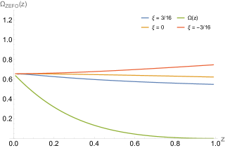
Figure 12: $\Omega_{{\textrm{\tiny{ZEFO}}}}$ (143) computed using the difference in expectation values of the SET between the Hartle-Hawking and Boulware states (blue, red and yellow curves, corresponding to three values of the coupling constant $\xi$), and $\Omega_{{\textrm{\tiny{ZEFO,RKT}}}}$ computed using the RKT approximation to the SET (green curve). The space-time and other scalar field parameters are as in Fig. 4.

In Fig. 12 we plot our results for $\Omega_{{\textrm{\tiny{ZEFO}}}}$ computed using both the difference in SET expectation values between the Hartle-Hawking and Boulware states and the RKT approximation to the SET (green curve). The RKT quantity $\Omega_{{\textrm{\tiny{ZEFO,RKT}}}}$ is computed in App. B, and found to be equal to $\Omega(r)$ (172). Therefore, in the RKT approximation, for a fixed value of the radial coordinate $r$, the gas of particles is rotating with the same angular speed as a ZAMO at the same radius. We see that $\Omega_{{\textrm{\tiny{ZEFO,RKT}}}}$ decreases rapidly as we move away from the horizon, and tends to zero at infinity.

In Fig. 12 we show our results for $\Omega_{{\textrm{\tiny{ZEFO}}}}$ for three values of the constant $\xi$ coupling the scalar field to the Ricci scalar curvature. For the other values of the coupling constant considered in Figs. 10 and 11, namely $\xi=1$ and $\xi=2$, we are unable to obtain physically reasonable values of $\Omega_{{\textrm{\tiny{ZEFO}}}}$, due to the quantity $A_{{\textrm{\tiny{ZEFO}}}}$ (142a) passing through zero between the event horizon and infinity.

For the values of $\xi$ considered in Fig. 12, on the horizon, $\Omega_{{\textrm{\tiny{ZEFO}}}}=\Omega_{{\textrm{\tiny{ZAMO}}}}=\Omega_{+}$ (18) as expected and the thermal distribution is rotating with the same angular speed as the event horizon. Away from the horizon, it can be seen in Fig. 12 that $\Omega_{{\textrm{\tiny{ZEFO}}}}$ has values close to (but not exactly equal to) $\Omega_{+}$, and, in particular, is significantly larger than the rate of rotation of a ZAMO, $\Omega(r)$. For $\xi=0$ (minimal coupling) and $\xi=3/16$ (conformal coupling) we find that $\Omega_{{\textrm{\tiny{ZEFO}}}}$ decreases slightly with increasing distance from the horizon, while for $\xi=-3/16$ it can be seen that $\Omega_{{\textrm{\tiny{ZEFO}}}}$ slightly increases as the radial coordinate increases. We deduce that the difference in SET expectation values between the Hartle-Hawking and Boulware states corresponds to a thermal distribution of particles almost (but not quite) rigidly-rotating with the angular speed of the event horizon.

On a Kerr black hole, a state rigidly-rotating with the same angular speed as the event horizon would be divergent on the speed-of-light surface [105]. This is not a concern in our situation, as we are assuming that the black hole rotates sufficiently slowly there there is no speed-of-light surface. Furthermore, it is clear from Fig. 12 that the thermal distribution is not exactly rigidly-rotating. Similar results were obtained for the corresponding thermal distribution of a quantum scalar [28], fermion [103] and electromagnetic [102] field on a Kerr space-time. For Kerr black holes, it is also found in [28, 102, 103] that $\Omega_{{\textrm{\tiny{ZEFO}}}}$ is significantly different from $\Omega_{{\textrm{\tiny{ZAMO}}}}$, as is the case in our set-up.

VI Conclusions

In this paper we have studied the canonical quantization of a scalar field on a background Myers-Perry-AdS black hole in five space-time dimensions. We have set the two angular momentum parameters in the metric to be equal, which results in a geometry with enhanced symmetry compared to the generic case. We assume that the angular momentum of the black hole is sufficiently small that there is no speed-of-light surface and there exists a Killing vector which is time-like everywhere outside the event horizon. In this case classical superradiance is absent and there are no unstable scalar field modes. We thus avoid the complexities of canonical quantization in the presence of classical superradiance [24, 83] and can readily construct a Boulware state $|{\mathrm{B}}\rangle$ and a Hartle-Hawking state $|{\mathrm{H}}\rangle$.

We compute the differences in expectation values of the vacuum polarization (the square of the field operator) and the SET operator between these two states, which have the advantage of not requiring renormalization. We compared these differences with approximations to these quantities derived in RKT, in which the quantum field is modelled as a thermal gas of particles.

The RKT approach only gives an analytic approximation to the difference in expectation values between the Hartle-Hawking and Boulware states, and furthermore we have found that quantum corrections to this difference in expectation values cannot be ignored. To find an approximation for the expectation values in either of these states (or a more accurate approximation to the difference between them), a more sophisticated approach (analogous to say, the Brown-Ottewill-Page [106, 107], DeWitt-Schwinger [108] or Polyakov [109] approximations in four space-time dimensions) would be required. Such approaches may enable the backreaction of the quantum field on the space-time geometry to be studied without recourse to a full computation of the renormalized SET (see comments below on this), see for example [110, 111, 112, 113, 114, 115, 116] for work on static, spherically symmetric black hole space-times along these lines.

Notwithstanding the simplifications afforded by the enhanced symmetry of the background space-time, our numerical computations are rather time-consuming. Consequently, we have presented results for one particular choice of the set of parameters of the model, which are the black hole mass parameter $M$, the angular momentum parameter $a$, and the scalar field effective mass $\nu$ (33). It would be interesting the explore the effect of varying these parameters on the quantum field expectation values, but this would require the development of a more efficient numerical method.

Since the black holes considered here are asymptotically-AdS, it is necessary to apply boundary conditions to the scalar field in order to have a well-defined quantum field theory. In this work, we have applied only the simplest (Dirichlet) boundary conditions to the field, for which the scalar field modes tend to zero as quickly as possible far from the black hole. While Dirichlet boundary conditions are the most widely employed in the literature, studies of the renormalized vacuum polarization in pure AdS in three and four dimensions [91, 92] has revealed that Neumann rather than Dirichlet boundary conditions give the generic behaviour of the vacuum polarization at the space-time boundary. Considering more general Robin boundary conditions changes the behaviour of both the vacuum polarization [91, 92] and SET [117, 118] in pure AdS space-time, and the vacuum polarization on asymptotically-AdS black holes in four dimensions [119] (the corresponding SET for Robin boundary conditions has yet to be computed). It would therefore also be interesting to explore the effect of different boundary conditions on the expectation values on the black hole space-times studied in this paper.

Our analysis has considered only the region exterior to the event horizon of the black hole, where both the Hartle-Hawking and Boulware states can be defined. We expect that the Boulware state is divergent at the event horizon, but that it should be possible to extend the construction of the Hartle-Hawking state into the black hole interior. For a four-dimensional Kerr black hole, there is no Hartle-Hawking state [26] to extend into the black hole interior, but the Unruh state has been constructed inside the event horizon [120]. A number of recent papers (see, for example, [121, 122, 123, 124, 125, 126]) have studied the properties of expectation values on the interiors of rotating black holes, paying particular attention to the region close to the inner horizon. A notable exception of a rotating black hole having a Hartle-Hawking state for which expectation values have been computed in the black hole interior is the three-dimensional BTZ black hole [17, 18, 19, 127], where again the behaviour at the inner horizon has been a particular focus of investigation.

Work to date on a Hartle-Hawking state on a black hole interior in four dimensions is restricted to spherically symmetric black holes (see, for example, [128] for the construction of $|{\rm{H}}\rangle$ inside a Reissner-Nordström black hole). The properties of expectation values on the interior of spherically symmetric black holes have attracted a good deal of attention in recent years (a selection of references is [129, 130, 131, 132, 133, 134, 123, 135, 136, 137]). A particular focus has been the behaviour of these quantities near the inner (Cauchy) horizon. In general, the expectation value of the SET for a quantum field diverges at the inner horizon, with a rate of divergence which is larger than the corresponding classical SET for classical perturbations [131, 132, 133, 136]. Thus quantum perturbations can restore cosmic censorship in the case of those Reissner-Nordström-de Sitter black holes for which classical perturbations do not blow up at the Cauchy horizon [131, 133].

One motivation for our work was the proof [34] of the existence of a Hartle-Hawking state for a four-dimensional stationary black hole possessing a Killing vector time-like everywhere outside the event horizon. We conjecture that a corresponding result holds for the black holes considered in this paper, although it should be emphasized that our construction of the state $|{\rm{H}}\rangle$ in this paper is not rigorous. To lend support to this hypothesis, it would be interesting to compute the renormalized expectation value of the SET (and the vacuum polarization) of the quantum scalar field in the state $|{\rm{H}}\rangle$, and in particular to ascertain whether this is regular at the event horizon. Such work would be a necessary precursor to any detailed investigation of the properties of the state $|{\rm{H}}\rangle$ on the black hole interior. We anticipate that significant technical challenges would arise in attempting to perform such a calculation. Of the recent methodologies for computing renormalized expectation values in the region exterior to a black hole event horizon, the “pragmatic mode sum” approach has been successful on the four-dimensional Kerr black hole [14]. However, this approach has, to date, only been employed on four-dimensional black holes, and it remains to be seen whether this would be practical to implement in higher dimensions. In contrast, the “extended coordinates” approach has been successfully applied to find the vacuum polarization on spherically symmetric black holes in more than four dimensions [138, 139]. In our case, we would be interested in developing this methodology to both the renormalized SET and rotating black holes, either of which is likely to be rather nontrivial. We therefore leave this for future work.

Appendix A Addition theorems for spin-weighted spherical harmonics

Below we state the addition theorems for spin-weighted spherical harmonics which enable us to simplify the SET components in App. C. The results below are proven elsewhere [72]. All the results below are valid for $\ell$ a positive integer or half-integer, and all $s$ an integer or half-integer, such that $\ell=|s|,|s|+1,|s|+2,\ldots$.

The addition theorems we require are:

$$\sum_{m=-\ell}^{\ell}{}_{s}Y_{\ell}^{m*}(\theta,\varphi){}_{s}Y_{\ell}^{m}(\theta,\varphi) =\frac{2\ell+1}{4\pi},$$ (144a)

$$\sum_{m=-\ell}^{\ell}m{}_{s}Y_{\ell}^{m*}(\theta,\varphi){}_{s}Y_{\ell}^{m}(\theta,\varphi) =-\frac{\left(2\ell+1\right)s}{4\pi}\cos\theta,$$ (144b)

$$\sum_{m=-\ell}^{\ell}m^{2}{}_{s}Y_{\ell}^{m*}(\theta,\varphi){}_{s}Y_{\ell}^{m}(\theta,\varphi) =\frac{2\ell+1}{8\pi}{\mathfrak{C}},$$ (144c)

$$\sum_{m=-\ell}^{\ell}{}_{s}Y_{\ell}^{m*}(\theta,\varphi)\frac{\partial}{\partial\theta}{}_{s}Y_{\ell}^{m}(\theta,\varphi) =0,$$ (144d)

$$\sum_{m=-\ell}^{\ell}\frac{\partial}{\partial\theta}{}_{s}Y_{\ell}^{m*}(\theta,\varphi)\frac{\partial}{\partial\theta}{}_{s}Y_{\ell}^{m}(\theta,\varphi) =\frac{2\ell+1}{8\pi}\left(\ell^{2}+\ell-s^{2}\right),$$ (144e)

where

$${\mathfrak{C}}=\left(\ell^{2}+\ell-s^{2}\right)\sin^{2}\theta+2s^{2}\cos^{2}\theta.$$ (144f)

It is straightforward to check that in the case $s=0$ (ordinary spherical harmonics), the results (144) reduce to those in, for example, App. C of Ref. [83].

Since we have ${}_{s}Y_{\ell}^{m}(\theta,\varphi)=e^{im\varphi}{}_{s}{\widetilde{Y}}_{\ell}^{m}(\theta)$ (37), the addition theorems in (144) give

$$\sum_{m=-\ell}^{\ell}\left|{}_{s}{\widetilde{Y}}_{\ell}^{m}(\theta)\right|^{2} =\frac{2\ell+1}{4\pi},$$ (145a)

$$\sum_{m=-\ell}^{\ell}m\left|{}_{s}{\widetilde{Y}}_{\ell}^{m}(\theta)\right|^{2} =\frac{\left(2\ell+1\right)p}{8\pi}\cos\theta,$$ (145b)

$$\sum_{m=-\ell}^{\ell}m^{2}\left|{}_{s}{\widetilde{Y}}_{\ell}^{m}(\theta)\right|^{2} =\frac{2\ell+1}{8\pi}{\mathfrak{C}},$$ (145c)

$$\sum_{m=-\ell}^{\ell}{}_{s}{\widetilde{Y}}_{\ell}^{m*}(\theta){}_{s}{\widetilde{Y}}_{\ell}^{{}^{\prime}m}(\theta) =0,$$ (145d)

$$\sum_{m=-\ell}^{\ell}\left|{}_{s}{\widetilde{Y}}_{\ell}^{{}^{\prime}m}(\theta)\right|^{2} =\frac{2\ell+1}{32\pi}\left(4\ell^{2}+4\ell-p^{2}\right),$$ (145e)

where we have used the fact that $$s=-p/2 {\mathfrak{C}}$$ (39), and where (144f) is now

$${\mathfrak{C}}=\frac{1}{4}\left(4\ell^{2}+4\ell-p^{2}\right)\sin^{2}\theta+\frac{p^{2}}{2}\cos^{2}\theta.$$ (145f)

As a corollary of the results (145), we have

$$\sum_{m=-\ell}^{\ell}\left[p\cot\theta-2m\csc\theta\right]^{2}{}_{s}{\widetilde{Y}}_{\ell}^{m}(\theta)^{2}\\ =\frac{2\ell+1}{8\pi}\left(4\ell^{2}+4\ell-p^{2}\right).$$ (146)

Appendix B Relativistic kinetic theory analysis

In this appendix we derive an approximation to the SET on the space-time background (1), based on relativistic kinetic theory (RKT) [96]. We compare this approximation to our quantum SET in Sec. V.2.

We begin by defining a funfbein (or pentrad) ${\mathsf{e}}^{\sigma}_{(a)}$ adapted to the metric (1), where we use the notation $(a)$ to denote funfbein indices. The simplest way to construct the funfbein is to start with the basis of one-forms $\varpi^{(a)}$

$$\varpi^{(t)} =f(r)\,dt,$$ (147a)

$$\varpi^{(r)} =g(r)\,dr,$$ (147b)

$$\varpi^{(\theta)} =\frac{r}{2}\,d\theta,$$ (147c)

$$\varpi^{(\varphi)} =\frac{r}{2}\sin\theta\,d\varphi,$$ (147d)

$$\varpi^{(\psi)} =h(r)\left[d\psi+\frac{1}{2}\cos\theta\,d\varphi-\Omega(r)\,dt\right].$$ (147e)

It is straightforward to check that the one-forms (147) satisfy the orthonormality conditions:

$$\varpi^{(a)}_{\sigma}\varpi^{(b)}_{\rho}\eta_{(a)(b)}=g_{\sigma\rho},\qquad\varpi^{(a)}_{\sigma}\varpi^{(b)}_{\rho}g^{\sigma\rho}=\eta^{(a)(b)},$$ (148)

where $\eta^{(a)(b)}$ is the inverse Minkowski metric. The funfbein basis vectors ${\mathsf{e}}^{\sigma}_{(a)}$ are then given by

$${\mathsf{e}}^{\sigma}_{(a)}=g^{\sigma\rho}\eta_{(a)(b)}\varpi^{(b)}_{\rho},$$ (149)

and we find

$${\mathsf{e}}_{(t)} =-f(r)^{-1}\left[\partial_{t}+\Omega(r)\,\partial_{\psi}\right],$$ (150a)

$${\mathsf{e}}_{(r)} =g(r)^{-1}\partial_{r},$$ (150b)

$${\mathsf{e}}_{(\theta)} =2r^{-1}\partial_{\theta},$$ (150c)

$${\mathsf{e}}_{(\varphi)} =r^{-1}\left[2\csc\theta\,\partial_{\varphi}+\cot\theta\,\partial_{\psi}\right],$$ (150d)

$${\mathsf{e}}_{(\psi)} =h(r)^{-1}\partial_{\psi}.$$ (150e)

The funfbein basis vectors (150) satisfy the orthonormality conditions

$${\mathsf{e}}_{(a)}^{\sigma}{\mathsf{e}}_{(b)}^{\rho}\eta^{(a)(b)}=g^{\sigma\rho},\qquad{\mathsf{e}}_{(a)}^{\sigma}{\mathsf{e}}_{(b)}^{\rho}g_{\sigma\rho}=\eta_{(a)(b)}.$$ (151)

We model our scalar field as a relativistic gas of noninteracting particles of mass $\mu_{{\textrm{\tiny{RKT}}}}$, in thermal equilibrium at rest in the orthonormal frame defined by the funfbein (147). In five space-time dimensions, the Bose-Einstein distribution function ${\mathsf{f}}$ is [140]

$${\mathsf{f}}=\frac{1}{\left(2\pi\right)^{4}}\left[\exp\left(-\beta_{{\textrm{\tiny{RKT}}}}{\hat{u}}\cdot{\hat{p}}\right)-1\right]^{-1},$$ (152)

where $\beta_{{\textrm{\tiny{RKT}}}}$ is the local inverse temperature, and ${\hat{u}}$ and ${\hat{p}}$ are, respectively, the five-velocity and five-momentum of the particles. We take the local inverse temperature to be that of an observer at rest in the corotating coordinates $(t,r,\theta,\varphi,\psi_{+})$, where the corotating angular coordinate $\psi_{+}$ is given by (20). This local inverse temperature is given by the Tolman relation [94, 95]

$$\beta_{{\textrm{\tiny{RKT}}}}=\beta_{0}{\sqrt{-g_{tt}^{+}}},$$ (153)

where $\beta_{0}$ is a fixed inverse temperature and $g_{tt}^{+}$ is the $(tt)$-component of the metric (21) in corotating coordinates. We take $\beta_{0}$ to be the inverse Hawking temperature $2\pi/\kappa_{+}$ of the black hole, where $\kappa_{+}$ is given in (19). Then, using (21), we find the local inverse temperature to be

$$\beta_{{\textrm{\tiny{RKT}}}}=\frac{2\pi}{\kappa_{+}}{\sqrt{f(r)^{2}-h(r)^{2}\left[\Omega(r)-\Omega_{+}\right]^{2}}}.$$ (154)

Near the event horizon, as $r\rightarrow r_{+}$, we have $f(r)\rightarrow 0$ and $\Omega(r)\rightarrow\Omega_{+}$, so that $\beta_{{\textrm{\tiny{RKT}}}}\rightarrow 0$. This means that the local temperature $\beta_{{\textrm{\tiny{RKT}}}}^{-1}$, as measured by an observer corotating with the event horizon tends to infinity. This is due to the fact that such an observer will have acceleration tending to infinity as the horizon is approached. Far from the black hole, we have, from (1b–1e), $f(r)\sim{\mathcal{O}}(r)$, $h(r)\sim{\mathcal{O}}(r)$ and $\Omega(r)\sim{\mathcal{O}}(r^{-4})$, so that $\beta_{{\textrm{\tiny{RKT}}}}\sim{\mathcal{O}}(r)$ and the local temperature $\beta_{{\textrm{\tiny{RKT}}}}^{-1}$ tends to zero. This is due to the fact that the black hole geometry is asymptotically AdS, and the local temperature in pure AdS tends to zero as the space-time boundary is approached [89].

For simplicity, we assume that the gas of particles is at rest relative to the funfbein (147), and therefore the five-velocity and five-momentum are

$${\hat{u}}^{(a)}=\delta^{(a)}_{(t)},\qquad{\hat{p}}=\mu_{{\textrm{\tiny{RKT}}}}{\hat{u}},$$ (155)

so that

$${\hat{u}}\cdot{\hat{p}}=-{\hat{p}}^{(t)},\qquad{\hat{p}}\cdot{\hat{p}}=-\mu_{{\textrm{\tiny{RKT}}}}^{2}.$$ (156)

The SET relative to the funfbein (147) is obtained by integrating the distribution function (152) over the spatial components of the five-momentum [141]:

$$T^{(a)(b)}_{{\textrm{\tiny{RKT}}}} =\int{\mathsf{f}}\,\frac{{\hat{p}}^{(a)}{\hat{p}}^{(b)}}{{\hat{p}}^{(t)}}\,d^{4}{\hat{p}}$$

$$=\left(E_{{\textrm{\tiny{RKT}}}}+P_{{\textrm{\tiny{RKT}}}}\right){\hat{u}}^{(a)}{\hat{u}}^{(b)}+P_{{\textrm{\tiny{RKT}}}}\eta^{(a)(b)},$$ (157)

where $E_{{\textrm{\tiny{RKT}}}}$ is the energy density and $P_{{\textrm{\tiny{RKT}}}}$ the pressure. Contracting (157) with ${\hat{u}}_{(a)}{\hat{u}}_{(b)}$ gives

$$E_{{\textrm{\tiny{RKT}}}}=\frac{1}{8\pi^{2}}\int_{{\mathsf{p}}=0}^{\infty}\frac{{\hat{p}}^{(t)}}{\exp\left(\beta_{{\textrm{\tiny{RKT}}}}{\hat{p}}^{(t)}\right)-1}\,{\mathsf{p}}^{3}\,d{\mathsf{p}},$$ (158a)

while contracting (157) with $$\eta_{(a)(b)}$$ gives

$$E_{{\textrm{\tiny{RKT}}}}-4P_{{\textrm{\tiny{RKT}}}}\\ =\frac{\mu^{2}_{{\textrm{\tiny{RKT}}}}}{8\pi^{2}}\int_{{\mathsf{p}}=0}^{\infty}\frac{1}{{\hat{p}}^{(t)}\left[\exp\left(\beta_{{\textrm{\tiny{RKT}}}}{\hat{p}}^{(t)}\right)-1\right]}\,{\mathsf{p}}^{3}\,d{\mathsf{p}},$$ (158b)

where ${\mathsf{p}}$ is the magnitude of the spatial part of the five-momentum ${\hat{p}}$, we have used (152, 156) and have performed the integrals over angular variables in momentum space.

The integrals in (158) are computed using the method outlined in, for example, [142]. First we expand the Bose-Einstein factor as:

$$\left[\exp\left(\beta_{{\textrm{\tiny{RKT}}}}{\hat{p}}^{(t)}\right)-1\right]^{-1}=\sum_{j=1}^{\infty}\exp\left(-j\beta_{{\textrm{\tiny{RKT}}}}{\hat{p}}^{(t)}\right).$$ (159)

Since $\left({\hat{p}}^{(t)}\right)^{2}-{\mathsf{p}}^{2}=\mu_{{\textrm{\tiny{RKT}}}}^{2}$, changing variables to ${\mathsf{X}}={\hat{p}}^{(t)}/\mu_{{\textrm{\tiny{RKT}}}}$ and ${\mathsf{Z}}=j\beta_{{\textrm{\tiny{RKT}}}}\mu_{{\textrm{\tiny{RKT}}}}$ gives the integrals

$$P_{{\textrm{\tiny{RKT}}}}=\frac{\mu_{{\textrm{\tiny{RKT}}}}^{5}}{32\pi^{2}}\sum_{j=1}^{\infty}\int_{{\mathsf{X}}=1}^{\infty}\left({\mathsf{X}}^{2}-1\right)^{2}\exp\left(-{\mathsf{X}}{\mathsf{Z}}\right)\,d{\mathsf{X}},$$ (160a)

$$E_{{\textrm{\tiny{RKT}}}}-4P_{{\textrm{\tiny{RKT}}}}=\frac{\mu_{{\textrm{\tiny{RKT}}}}^{5}}{8\pi^{2}}\sum_{j=1}^{\infty}\int_{{\mathsf{X}}=1}^{\infty}\left({\mathsf{X}}^{2}-1\right)\exp\left(-{\mathsf{X}}{\mathsf{Z}}\right)\,d{\mathsf{X}}.$$ (160b)

These are evaluated using the result

$$\int_{{\mathsf{X}}=1}^{\infty}\left(X^{2}-1\right)^{{\mathsf{v}}-\frac{1}{2}}e^{-{\mathsf{X}}{\mathsf{Z}}}\,d{\mathsf{X}}=\frac{2^{\mathsf{v}}\Gamma\left(\frac{1}{2}+{\mathsf{v}}\right)}{{\mathsf{Z}}^{\mathsf{v}}{\sqrt{\pi}}}K_{{\mathsf{v}}}({\mathsf{Z}}),$$ (161)

where $K_{{\mathsf{v}}}({\mathsf{Z}})$ is a modified Bessel function of the second kind. We then have

$$P_{{\textrm{\tiny{RKT}}}} =\frac{\mu_{{\textrm{\tiny{RKT}}}}^{5}}{4\pi^{2}}{\sqrt{\frac{2}{\pi}}}\sum_{j=1}^{\infty}\frac{K_{\frac{5}{2}}(j\beta_{{\textrm{\tiny{RKT}}}}\mu_{{\textrm{\tiny{RKT}}}})}{(j\beta_{{\textrm{\tiny{RKT}}}}\mu_{{\textrm{\tiny{RKT}}}})^{\frac{5}{2}}},$$ (162a)

$$E_{{\textrm{\tiny{RKT}}}}-4P_{{\textrm{\tiny{RKT}}}} =\frac{\mu_{{\textrm{\tiny{RKT}}}}^{5}}{4\pi^{2}}{\sqrt{\frac{2}{\pi}}}\sum_{j=1}^{\infty}\frac{K_{\frac{3}{2}}(j\beta_{{\textrm{\tiny{RKT}}}}\mu_{{\textrm{\tiny{RKT}}}})}{(j\beta_{{\textrm{\tiny{RKT}}}}\mu_{{\textrm{\tiny{RKT}}}})^{\frac{3}{2}}}.$$ (162b)

The particular modified Bessel functions in (162) take the simple form:

$$K_{\frac{3}{2}}({\mathsf{x}}) =e^{-{\mathsf{x}}}{\sqrt{\frac{\pi}{2{\mathsf{x}}}}}\left(1+\frac{1}{{\mathsf{x}}}\right),$$ (163a)

$$K_{\frac{5}{2}}({\mathsf{x}}) =e^{-{\mathsf{x}}}{\sqrt{\frac{\pi}{2{\mathsf{x}}}}}\left(1+\frac{3}{{\mathsf{x}}}+\frac{3}{{\mathsf{x}}^{2}}\right),$$ (163b)

and the resulting summations in (162) can be written in terms of polylogarithms:

$$\sum_{j=1}^{\infty}e^{-j{\mathsf{x}}}\left(j{\mathsf{x}}\right)^{-n}={\mathsf{x}}^{-n}\,{\mathrm{Li}}_{n}(e^{-{\mathsf{x}}}).$$ (163c)

The final answers are:

$$P_{{\textrm{\tiny{RKT}}}} =\frac{1}{4\pi^{2}\beta_{{\textrm{\tiny{RKT}}}}^{5}}\left[\left(\beta_{{\textrm{\tiny{RKT}}}}\mu_{{\textrm{\tiny{RKT}}}}\right)^{2}\,{\mathrm{Li}}_{3}({\mathsf{Y}})\right.$$

$$\qquad\left.+3\left(\beta_{{\textrm{\tiny{RKT}}}}\mu_{{\textrm{\tiny{RKT}}}}\right)\,{\mathrm{Li}}_{4}({\mathsf{Y}})\right.$$

$$\qquad\left.+3\,{\mathrm{Li}}_{5}({\mathsf{Y}})\right],$$ (164a)

$$E_{{\textrm{\tiny{RKT}}}}-4P_{{\textrm{\tiny{RKT}}}} =\frac{\mu_{{\textrm{\tiny{RKT}}}}^{2}}{4\pi^{2}\beta_{{\textrm{\tiny{RKT}}}}^{3}}\left[\left(\beta_{{\textrm{\tiny{RKT}}}}\mu_{{\textrm{\tiny{RKT}}}}\right)\,{\mathrm{Li}}_{2}({\mathsf{Y}})\right.$$

$$\qquad\left.+{\mathrm{Li}}_{3}({\mathsf{Y}})\right],$$ (164b)

where

$${\mathsf{Y}}=\exp\left(-\beta_{{\textrm{\tiny{RKT}}}}\mu_{{\textrm{\tiny{RKT}}}}\right).$$ (164c)

In the massless limit $\mu_{{\textrm{\tiny{RKT}}}}=0$, these results reduce to

$$E_{{\textrm{\tiny{RKT}}}}=4P_{{\textrm{\tiny{RKT}}}}=\frac{3\zeta(5)}{4\pi^{2}\beta_{{\textrm{\tiny{RKT}}}}^{5}}.$$ (165)

It is notable that, in (165), both $E_{{\textrm{\tiny{RKT}}}}$ and $P_{{\textrm{\tiny{RKT}}}}$ are proportional to the fifth power of the temperature $\beta_{{\textrm{\tiny{RKT}}}}^{-1}$, whereas in four space-time dimensions they are proportional to $\beta_{{\textrm{\tiny{RKT}}}}^{-4}$.

The behaviour of the quantities (164) near the event horizon (where $\beta_{{\textrm{\tiny{RKT}}}}\rightarrow 0$) and at infinity (where $\beta_{{\textrm{\tiny{RKT}}}}\rightarrow\infty$) can be deduced using the asymptotic behaviour of the polylogarithm function:

$${\mathrm{Li}}_{n}(e^{-{\mathsf{x}}})\sim\begin{cases}\zeta(n),&{\mathsf{x}}\rightarrow 0,\\ e^{-{\mathsf{x}}},&{\mathsf{x}}\rightarrow\infty,\end{cases}$$ (166)

where $\zeta(n)$ is the Riemann-zeta function. We therefore find, as $\beta_{{\textrm{\tiny{RKT}}}}\rightarrow 0$,

$$P_{{\textrm{\tiny{RKT}}}} \sim\frac{3\zeta(5)}{4\pi^{2}\beta_{{\textrm{\tiny{RKT}}}}^{5}},$$ (167a)

$$E_{{\textrm{\tiny{RKT}}}}-4P_{{\textrm{\tiny{RKT}}}} \sim\frac{\mu_{{\textrm{\tiny{RKT}}}}^{2}\zeta(3)}{4\pi^{2}\beta_{{\textrm{\tiny{RKT}}}}^{3}},$$ (167b)

while, as $$\beta_{{\textrm{\tiny{RKT}}}}\rightarrow\infty$$, we have

$$P_{{\textrm{\tiny{RKT}}}} \sim\frac{\mu_{{\textrm{\tiny{RKT}}}}^{2}\exp\left(-\beta_{{\textrm{\tiny{RKT}}}}\mu_{{\textrm{\tiny{RKT}}}}\right)}{4\pi^{2}\beta_{{\textrm{\tiny{RKT}}}}^{3}},$$ (167c)

$$E_{{\textrm{\tiny{RKT}}}}-4P_{{\textrm{\tiny{RKT}}}} \sim\frac{\mu_{{\textrm{\tiny{RKT}}}}^{3}\exp\left(-\beta_{{\textrm{\tiny{RKT}}}}\mu_{{\textrm{\tiny{RKT}}}}\right)}{4\pi^{2}\beta_{{\textrm{\tiny{RKT}}}}^{2}}.$$ (167d)

As expected, the high-temperature results ($\beta_{{\textrm{\tiny{RKT}}}}\rightarrow 0$) are independent of the mass $\mu_{{\textrm{\tiny{RKT}}}}$, with both the energy density and pressure proportional to the fifth power of the temperature as in the massless case, while in the low temperature limit ($\beta_{{\textrm{\tiny{RKT}}}}\rightarrow\infty$), both the energy density and pressure tend to zero exponentially fast.

To aid comparison with our results in Sec. V.2, we write the SET (157) in coordinate components using

$$T_{{\textrm{\tiny{RKT}}}}^{\rho\sigma}={\mathsf{e}}_{(a)}^{\rho}{\mathsf{e}}_{(b)}^{\sigma}T_{{\textrm{\tiny{RKT}}}}^{(a)(b)},$$ (168)

which yields the components

$$T_{{\textrm{\tiny{RKT}}}}^{tt} =f(r)^{-2}E_{{\textrm{\tiny{RKT}}}},$$ (169a)

$$T_{{\textrm{\tiny{RKT}}}}^{tr} =0,$$ (169b)

$$T_{{\textrm{\tiny{RKT}}}}^{t\theta} =0,$$ (169c)

$$T_{{\textrm{\tiny{RKT}}}}^{t\varphi} =0,$$ (169d)

$$T_{{\textrm{\tiny{RKT}}}}^{t\psi} =f(r)^{-2}\Omega(r)E_{{\textrm{\tiny{RKT}}}},$$ (169e)

$$T_{{\textrm{\tiny{RKT}}}}^{rr} =g(r)^{-2}P_{{\textrm{\tiny{RKT}}}},$$ (169f)

$$T_{{\textrm{\tiny{RKT}}}}^{r\theta} =0,$$ (169g)

$$T_{{\textrm{\tiny{RKT}}}}^{r\varphi} =0,$$ (169h)

$$T_{{\textrm{\tiny{RKT}}}}^{r\psi} =0,$$ (169i)

$$T_{{\textrm{\tiny{RKT}}}}^{\theta\theta} =4r^{-2}P_{{\textrm{\tiny{RKT}}}},$$ (169j)

$$T_{{\textrm{\tiny{RKT}}}}^{\theta\varphi} =0,$$ (169k)

$$T_{{\textrm{\tiny{RKT}}}}^{\theta\psi} =0,$$ (169l)

$$T_{{\textrm{\tiny{RKT}}}}^{\varphi\varphi} =4r^{-2}P_{{\textrm{\tiny{RKT}}}}\csc^{2}\theta,$$ (169m)

$$T_{{\textrm{\tiny{RKT}}}}^{\varphi\psi} =-2r^{-2}P_{{\textrm{\tiny{RKT}}}}\cot\theta\csc\theta,$$ (169n)

$$T_{{\textrm{\tiny{RKT}}}}^{\psi\psi} =f(r)^{-2}\Omega(r)^{2}E_{{\textrm{\tiny{RKT}}}}$$

$$\qquad+\left[h(r)^{-2}+r^{-2}\cot^{2}\theta\right]P_{{\textrm{\tiny{RKT}}}}.$$ (169o)

It can be seen that the coordinate components (169) have exactly the same form as (121), with the following functions ${\mathcal{F}}_{{\textrm{\tiny{RKT}}}}^{\bullet\bullet}(r)$:

$${\mathcal{F}}_{{\textrm{\tiny{RKT}}}}^{tt}(r) =f(r)^{-2}E_{{\textrm{\tiny{RKT}}}},$$ (170a)

$${\mathcal{F}}_{{\textrm{\tiny{RKT}}}}^{tr}(r) =0,$$ (170b)

$${\mathcal{F}}_{{\textrm{\tiny{RKT}}}}^{t\psi}(r) =f(r)^{-2}\Omega(r)E_{{\textrm{\tiny{RKT}}}},$$ (170c)

$${\mathcal{F}}_{{\textrm{\tiny{RKT}}}}^{rr}(r) =g(r)^{-2}P_{{\textrm{\tiny{RKT}}}},$$ (170d)

$${\mathcal{F}}_{{\textrm{\tiny{RKT}}}}^{r\psi}(r) =0,$$ (170e)

$${\mathcal{F}}_{{\textrm{\tiny{RKT}}}}^{\theta\theta}(r) =4r^{-2}P_{{\textrm{\tiny{RKT}}}},$$ (170f)

$${\mathcal{F}}_{{\textrm{\tiny{RKT}}}}^{\psi\psi}(r) =f(r)^{-2}\Omega(r)^{2}E_{{\textrm{\tiny{RKT}}}}$$

$$\qquad+\left[h(r)^{-2}-r^{-2}\right]P_{{\textrm{\tiny{RKT}}}},$$ (170g)

where we have used the trigonometric identity

$$\cot^{2}\theta+1=\csc^{2}\theta.$$ (171)

Finally, we can use the coordinate components (169) and the method of [102, 103] (outlined in Sec. V.2.3) to find the value of the angular speed $\Omega_{{\textrm{\tiny{ZEFO,RKT}}}}$ for an observer who sees no angular flux of energy when the SET is given by the RKT approximation. A straightforward calculation gives

$$\Omega_{{\textrm{\tiny{ZEFO,RKT}}}}=\Omega(r).$$ (172)

Therefore, in the RKT approximation, a ZEFO is also a ZAMO [104], in other words, an observer who sees no angular flux of energy in the thermal gas of particles (that is, a ZEFO), is also an observer having zero angular momentum about the axis of rotation of the black hole (that is, a ZAMO). This is unsurprising; we have defined our thermal gas of particles to be at rest in the orthonormal frame given by the funfbein (150), which is exactly the frame (139) with $\mho=\Omega_{{\textrm{\tiny{ZEFO,RKT}}}}=\Omega(r)$ (140).

Appendix C Stress-energy tensor components

In this appendix we give explicit expressions for the components of the classical SET (34) evaluated for a scalar field mode (35) with angular function (37). Since these expressions are fairly lengthy, we omit the indices on the radial and angular functions. In terms of the metric functions $f(r)$, $g(r)$, $h(r)$ and $\Omega(r)$ (1b–1e), the SET components are:

$${}^{\aleph}T_{tt} =\omega^{2}\left|X(r)\right|^{2}{\widetilde{Y}}(\theta)^{2}+\frac{2\xi}{g(r)^{2}}\left[f(r)f^{\prime}(r)-h(r)\Omega(r)\frac{d}{dr}\left\{h(r)\Omega(r)\right\}\right]\Re\left\{X^{*}(r)X^{\prime}(r)\right\}{\widetilde{Y}}(\theta)^{2}$$

$$\qquad-\left[f(r)^{2}-h(r)^{2}\Omega(r)^{2}\right]{\mathfrak{Z}}(r,\theta),$$ (173a)

$${}^{\aleph}T_{tr} =-\omega\Im\left\{X^{*}(r)X^{\prime}(r)\right\}{\widetilde{Y}}(\theta)^{2},$$ (173b)

$${}^{\aleph}T_{t\theta} =0,$$ (173c)

$${}^{\aleph}T_{t\varphi} =-m\omega\left|X(r)\right|^{2}{\widetilde{Y}}(\theta)^{2}-\frac{2\xi}{r^{2}}h(r)^{2}\Omega(r)\left|X(r)\right|^{2}{\widetilde{Y}}^{\prime}(\theta){\widetilde{Y}}(\theta)\sin\theta$$

$$\qquad+\frac{\xi h(r)}{2g(r)^{2}}\left[h(r)\Omega^{\prime}(r)+2h^{\prime}(r)\Omega(r)\right]\Re\left\{X^{*}(r)X^{\prime}(r)\right\}{\widetilde{Y}}(\theta)^{2}\cos\theta-\frac{1}{2}h(r)^{2}\Omega(r){\mathfrak{Z}}(r,\theta)\cos\theta,$$ (173d)

$${}^{\aleph}T_{t\psi} =-p\omega\left|X(r)\right|^{2}{\widetilde{Y}}(\theta)^{2}+\frac{\xi h(r)}{g(r)^{2}}\left[h(r)\Omega^{\prime}(r)+2h^{\prime}(r)\Omega(r)\right]\Re\left\{X^{*}(r)X^{\prime}(r)\right\}{\widetilde{Y}}(\theta)^{2}-h(r)^{2}\Omega(r){\mathfrak{Z}}(r,\theta),$$ (173e)

$${}^{\aleph}T_{rr} =\left(1-2\xi\right)\left|X^{\prime}(r)\right|^{2}{\widetilde{Y}}(\theta)^{2}-2\xi g(r)^{2}\left[\frac{1}{r^{2}h(r)^{2}}\left\{p^{2}r^{2}+\left(4\lambda+r^{2}\nu^{2}\right)h(r)^{2}\right\}-\frac{1}{f(r)^{2}}\left\{\omega-p\Omega(r)\right\}^{2}\right]\left|X(r)\right|^{2}{\widetilde{Y}}(\theta)^{2}$$

$$\qquad+2\xi\left[\frac{f^{\prime}(r)}{f(r)}+\frac{2h(r)+rh^{\prime}(r)}{rh(r)}\right]\Re\left\{X^{*}(r)X^{\prime}(r)\right\}{\widetilde{Y}}(\theta)^{2}+g(r)^{2}{\mathfrak{Z}}(r,\theta),$$ (173f)

$${}^{\aleph}T_{r\theta} =\left[\left(1-4\xi\right)\Re\left\{X^{*}(r)X^{\prime}(r)\right\}+\frac{2\xi}{r}\left|X(r)\right|^{2}\right]{\widetilde{Y}}^{\prime}(\theta){\widetilde{Y}}(\theta),$$ (173g)

$${}^{\aleph}T_{r\varphi} =m\Im\left\{X^{*}(r)X^{\prime}(r)\right\}{\widetilde{Y}}(\theta)^{2},$$ (173h)

$${}^{\aleph}T_{r\psi} =p\Im\left\{X^{*}(r)X^{\prime}(r)\right\}{\widetilde{Y}}(\theta)^{2},$$ (173i)

$${}^{\aleph}T_{\theta\theta} =\left(1-2\xi\right)\left|X(r)\right|^{2}{\widetilde{Y}}^{\prime}(\theta)^{2}-\frac{\xi r}{2g(r)^{2}}\Re\left\{X^{*}(r)X^{\prime}(r)\right\}{\widetilde{Y}}(\theta)^{2}+2\xi\left[\lambda-\frac{1}{4}\left(p\cot\theta-2m\csc\theta\right)^{2}\right]\left|X(r)\right|^{2}{\widetilde{Y}}(\theta)^{2}$$

$$\qquad+2\xi\cot\theta\left|X(r)\right|^{2}{\widetilde{Y}}^{\prime}(\theta){\widetilde{Y}}(\theta)+\frac{1}{4}r^{2}{\mathfrak{Z}}(r,\theta),$$ (173j)

$${}^{\aleph}T_{\theta\varphi} =0,$$ (173k)

$${}^{\aleph}T_{\theta\psi} =0,$$ (173l)

$${}^{\aleph}T_{\varphi\varphi} =m^{2}\left|X(r)\right|^{2}{\widetilde{Y}}(\theta)^{2}-\frac{\xi}{2g(r)^{2}}\left[r\sin^{2}\theta+h(r)h^{\prime}(r)\cos^{2}\theta\right]\Re\left\{X^{*}(r)X^{\prime}(r)\right\}{\widetilde{Y}}(\theta)^{2}$$

$$\qquad+\frac{\xi}{r^{2}}\left[h(r)^{2}-r^{2}\right]\left|X(r)\right|^{2}{\widetilde{Y}}^{\prime}(\theta){\widetilde{Y}}(\theta)\sin(2\theta)+\frac{1}{4}\left[r^{2}\sin^{2}\theta+h(r)^{2}\cos^{2}\theta\right]{\mathfrak{Z}}(r,\theta),$$ (173m)

$${}^{\aleph}T_{\varphi\psi} =mp\left|X(r)\right|^{2}{\widetilde{Y}}(\theta)^{2}-\frac{\xi h(r)h^{\prime}(r)}{g(r)^{2}}\Re\left\{X^{*}(r)X^{\prime}(r)\right\}{\widetilde{Y}}(\theta)^{2}\cos\theta+\frac{2\xi h(r)^{2}}{r^{2}}\left|X(r)\right|^{2}{\widetilde{Y}}^{\prime}(\theta){\widetilde{Y}}(\theta)\sin\theta$$

$$\qquad+\frac{1}{2}h(r)^{2}{\mathfrak{Z}}(r,\theta)\cos\theta,$$ (173n)

$${}^{\aleph}T_{\psi\psi} =p^{2}\left|X(r)\right|^{2}{\widetilde{Y}}(\theta)^{2}-\frac{2\xi h(r)h^{\prime}(r)}{g(r)^{2}}\Re\left\{X^{*}(r)X^{\prime}(r)\right\}{\widetilde{Y}}(\theta)^{2}+h(r)^{2}{\mathfrak{Z}}(r,\theta),$$ (173o)

where

$${\mathfrak{Z}}(r,\theta)= ~{}\left(2\xi-\frac{1}{2}\right)g^{\rho\sigma}\Phi_{;\rho}\Phi_{;\sigma}+\frac{1}{2}\left(4\xi-1\right)\mu^{2}\Phi^{2}+\xi R\left(2\xi-\frac{3}{10}\right)\Phi^{2}$$

$$= ~{}\left(2\xi-\frac{1}{2}\right)\left[\left\{\dfrac{p^{2}}{h(r)^{2}}+\dfrac{1}{r^{2}}\left[p\cot\theta-2m\csc\theta\right]^{2}-\dfrac{1}{f(r)^{2}}\left[\omega-p\Omega(r)\right]^{2}\right\}\left|X(r)\right|^{2}{\widetilde{Y}}(\theta)^{2}\right.$$

$$\qquad\left.+\dfrac{1}{g(r)^{2}}\left|X^{\prime}(r)\right|^{2}{\widetilde{Y}}(\theta)^{2}+\dfrac{4}{r^{2}}\left|X(r)\right|^{2}{\widetilde{Y}}^{\prime}(\theta)^{2}\right]+\left[\frac{1}{2}\left(4\xi-1\right)\mu^{2}+\xi R\left(2\xi-\frac{3}{10}\right)\right]\left|X(r)\right|^{2}{\widetilde{Y}}(\theta)^{2}.$$ (173p)

In (173), the radial functions $X(r)$ depend on the frequency $\omega$ and the azimuthal quantum number $p\in{\mathbb{Z}}$, while the angular functions ${\widetilde{Y}}(\theta)$ depend on the quantum number $m=-\ell,-\ell+1,\ldots,\ell-1,\ell$, the spin $s=-p/2$ (39) and the quantum number $\ell=|s|,|s|+1,|s|+2,\ldots$.

We now use the addition theorems for the spin-weighted spherical harmonics from App. A (145) to perform the sum over $m$ in each of the SET components. We define new quantities $t_{\mu\nu}$ by

$$\sum_{m=-\ell}^{\ell}{}^{\aleph}T_{\mu\nu}=\frac{2\ell+1}{4\pi}t_{\mu\nu}$$ (174)

where ${}^{\aleph}T_{\mu\nu}$ are the components given in (173). A further simplification arises from the fact that, for our particular modes (66), we have $\Im\left\{X^{*}(r)X^{\prime}(r)\right\}=0$. Then we have

$$t_{tt} =\omega^{2}\left|X(r)\right|^{2}+\frac{2\xi}{g(r)^{2}}\left[f(r)f^{\prime}(r)-h(r)\Omega(r)\frac{d}{dr}\left\{h(r)\Omega(r)\right\}\right]\Re\left\{X^{*}(r)X^{\prime}(r)\right\}-\left[f(r)^{2}-h(r)^{2}\Omega(r)^{2}\right]{\widetilde{{\mathfrak{Z}}}}(r),$$ (175a)

$$t_{tr} =0,$$ (175b)

$$t_{t\theta} =0,$$ (175c)

$$t_{t\varphi} =\left\{\frac{1}{2}p\omega\left|X(r)\right|^{2}+\frac{\xi h(r)}{2g(r)^{2}}\left[h(r)\Omega^{\prime}(r)+2h^{\prime}(r)\Omega(r)\right]\Re\left\{X^{*}(r)X^{\prime}(r)\right\}-\frac{1}{2}h(r)^{2}\Omega(r){\widetilde{{\mathfrak{Z}}}}(r)\right\}\cos\theta,$$ (175d)

$$t_{t\psi} =-p\omega\left|X(r)\right|^{2}+\frac{\xi h(r)}{g(r)^{2}}\left[h(r)\Omega^{\prime}(r)+2h^{\prime}(r)\Omega(r)\right]\Re\left\{X^{*}(r)X^{\prime}(r)\right\}-h(r)^{2}\Omega(r){\widetilde{{\mathfrak{Z}}}}(r),$$ (175e)

$$t_{rr} =\left(1-2\xi\right)\left|X^{\prime}(r)\right|^{2}-2\xi g(r)^{2}\left[\frac{1}{r^{2}h(r)^{2}}\left\{p^{2}r^{2}+\left(4\lambda+r^{2}\nu^{2}\right)h(r)^{2}\right\}-\frac{1}{f(r)^{2}}\left\{\omega-p\Omega(r)\right\}^{2}\right]\left|X(r)\right|^{2}$$

$$\qquad+2\xi\left[\frac{f^{\prime}(r)}{f(r)}+\frac{2h(r)+rh^{\prime}(r)}{rh(r)}\right]\Re\left\{X^{*}(r)X^{\prime}(r)\right\}+g(r)^{2}{\widetilde{{\mathfrak{Z}}}}(r),$$ (175f)

$$t_{r\theta} =0,$$ (175g)

$$t_{r\varphi} =0,$$ (175h)

$$t_{r\psi} =0,$$ (175i)

$$t_{\theta\theta} =\frac{1}{8}\left(1-4\xi\right)\left(4\ell^{2}+4\ell-p^{2}\right)\left|X(r)\right|^{2}+2\xi\lambda\left|X(r)\right|^{2}-\frac{\xi r}{2g(r)^{2}}\Re\left\{X^{*}(r)X^{\prime}(r)\right\}+\frac{1}{4}r^{2}{\widetilde{{\mathfrak{Z}}}}(r),$$ (175j)

$$t_{\theta\varphi} =0,$$ (175k)

$$t_{\theta\psi} =0,$$ (175l)

$$t_{\varphi\varphi} =\frac{1}{2}{\mathfrak{C}}\left|X(r)\right|^{2}{\widetilde{Y}}(\theta)^{2}-\frac{\xi}{2g(r)^{2}}\left[r\sin^{2}\theta+h(r)h^{\prime}(r)\cos^{2}\theta\right]\Re\left\{X^{*}(r)X^{\prime}(r)\right\}+\frac{1}{4}\left[r^{2}\sin^{2}\theta+h(r)^{2}\cos^{2}\theta\right]{\widetilde{{\mathfrak{Z}}}}(r),$$ (175m)

$$t_{\varphi\psi} =-\left\{\frac{1}{2}p^{2}\left|X(r)\right|^{2}+\frac{\xi h(r)h^{\prime}(r)}{g(r)^{2}}\Re\left\{X^{*}(r)X^{\prime}(r)\right\}-\frac{1}{2}h(r)^{2}{\widetilde{{\mathfrak{Z}}}}(r)\right\}\cos\theta,$$ (175n)

$$t_{\psi\psi} =p^{2}\left|X(r)\right|^{2}-\frac{2\xi h(r)h^{\prime}(r)}{g(r)^{2}}\Re\left\{X^{*}(r)X^{\prime}(r)\right\}+h(r)^{2}{\widetilde{{\mathfrak{Z}}}}(r),$$ (175o)

where $${\mathfrak{C}}$$ is given by (145f) and

$${\widetilde{{\mathfrak{Z}}}}(r)=\left\{\dfrac{p^{2}}{h(r)^{2}}+\dfrac{1}{2r^{2}}\left(4\ell^{2}+4\ell-p^{2}\right)-\dfrac{1}{f(r)^{2}}\left[\omega-p\Omega(r)\right]^{2}\right.\\ \left.+\frac{1}{2}\left(4\xi-1\right)\mu^{2}+\xi R\left(2\xi-\frac{3}{10}\right)\right\}\left|X(r)\right|^{2}+\dfrac{1}{g(r)^{2}}\left|X^{\prime}(r)\right|^{2}+\dfrac{1}{2r^{2}}\left(4\ell^{2}+4\ell-p^{2}\right)\left|X(r)\right|^{2},$$ (175p)

and we have simplified using the result (40). It can be seen from (175) that all the dependence on the angle $\theta$ is now determined in closed form.

We now wish to compare the components (175) with the form of the SET (121) derived from symmetry principles. Using the metric (1) to lower the indices on (121), we find

$$\langle{\hat{T}}_{tt}\rangle =\left[f(r)^{2}-h(r)^{2}\Omega(r)^{2}\right]^{2}{\mathcal{F}}^{tt}(r)+2h(r)^{2}\Omega(r)\left[f(r)^{2}-h(r)^{2}\Omega(r)^{2}\right]{\mathcal{F}}^{t\psi}(r)+h(r)^{4}\Omega(r)^{2}{\mathcal{F}}^{\psi\psi}(r)$$

$$\qquad+\frac{1}{4}h(r)^{4}\Omega(r)^{2}{\mathcal{F}}^{\theta\theta}(r),$$ (176a)

$$\langle{\hat{T}}_{tr}\rangle =-g(r)^{2}\left[f(r)^{2}-h(r)^{2}\Omega(r)^{2}\right]{\mathcal{F}}^{tr}(r)-g(r)^{2}h(r)^{2}\Omega(r){\mathcal{F}}^{r\psi}(r),$$ (176b)

$$\langle{\hat{T}}_{t\theta}\rangle =0,$$ (176c)

$$\langle{\hat{T}}_{t\varphi}\rangle =\frac{1}{2}h(r)^{2}\bigg{\{}\Omega(r)\left[f(r)^{2}-h(r)^{2}\Omega(r)^{2}\right]{\mathcal{F}}^{tt}(r)-\left[f(r)^{2}-2h(r)^{2}\Omega(r)^{2}\right]{\mathcal{F}}^{t\psi}(r)-h(r)^{2}\Omega(r){\mathcal{F}}^{\psi\psi}(r)$$

$$\qquad-\frac{1}{4}h(r)^{2}\Omega(r){\mathcal{F}}^{\theta\theta}(r)\bigg{\}}\cos\theta,$$ (176d)

$$\langle{\hat{T}}_{t\psi}\rangle =h(r)^{2}\bigg{\{}\Omega(r)\left[f(r)^{2}-h(r)^{2}\Omega(r)^{2}\right]{\mathcal{F}}^{tt}(r)-\left[f(r)^{2}-2h(r)^{2}\Omega(r)^{2}\right]{\mathcal{F}}^{t\psi}(r)-h(r)^{2}\Omega(r){\mathcal{F}}^{\psi\psi}$$

$$\qquad-\frac{1}{4}h(r)^{2}\Omega(r){\mathcal{F}}^{\theta\theta}(r)\bigg{\}},$$ (176e)

$$\langle{\hat{T}}_{rr}\rangle =g(r)^{4}{\mathcal{F}}^{rr}(r),$$ (176f)

$$\langle{\hat{T}}_{r\theta}\rangle =0,$$ (176g)

$$\langle{\hat{T}}_{r\varphi}\rangle =\frac{1}{2}g(r)^{2}h(r)^{2}\left\{{\mathcal{F}}^{r\psi}(r)-\Omega(r){\mathcal{F}}^{tr}(r)\right\}\cos\theta,$$ (176h)

$$\langle{\hat{T}}_{r\psi}\rangle =g(r)^{2}h(r)^{2}\left\{{\mathcal{F}}^{r\psi}(r)-\Omega(r){\mathcal{F}}^{tr}(r)\right\},$$ (176i)

$$\langle{\hat{T}}_{\theta\theta}\rangle =\frac{r^{4}}{16}{\mathcal{F}}^{\theta\theta}(r),$$ (176j)

$$\langle{\hat{T}}_{\theta\varphi}\rangle =0,$$ (176k)

$$\langle{\hat{T}}_{\theta\psi}\rangle =0,$$ (176l)

$$\langle{\hat{T}}_{\varphi\varphi}\rangle =\frac{1}{4}h(r)^{4}\left\{\Omega(r)^{2}{\mathcal{F}}^{tt}(r)-2\Omega(r){\mathcal{F}}^{t\psi}(r)+{\mathcal{F}}^{\psi\psi}(r)\right\}\cos^{2}\theta+\frac{1}{16}\left[h(r)^{4}\cos^{2}\theta+r^{4}\sin^{2}\theta\right]{\mathcal{F}}^{\theta\theta}(r),$$ (176m)

$$\langle{\hat{T}}_{\varphi\psi}\rangle =\frac{1}{2}h(r)^{4}\left\{\Omega(r)^{2}{\mathcal{F}}^{tt}(r)-2\Omega(r){\mathcal{F}}^{t\psi}(r)+{\mathcal{F}}^{\psi\psi}(r)\right\}\cos\theta+\frac{1}{8}h(r)^{4}{\mathcal{F}}^{\theta\theta}(r)\cos\theta,$$ (176n)

$$\langle{\hat{T}}_{\psi\psi}\rangle =h(r)^{4}\left\{\Omega(r)^{2}{\mathcal{F}}^{tt}(r)-2\Omega(r){\mathcal{F}}^{t\psi}(r)+{\mathcal{F}}^{\psi\psi}(r)\right\}+\frac{1}{4}h(r)^{4}{\mathcal{F}}^{\theta\theta}(r),$$ (176o)

from which it is clear that the dependence on the angle $\theta$ in all components is of the same form. Let ${\mathfrak{F}}^{\bullet\bullet}$ be the classical mode contribution to ${\mathcal{F}}^{\bullet\bullet}$ arising from the scalar field mode (35), with the sum over $m$ completed. To find the ${\mathfrak{F}}^{\bullet\bullet}$, it is simplest to use the inverse metric (4) to raise both indices on the components in (175) and then compare with (121). This gives

$${\mathfrak{F}}^{tt}(r) =\frac{1}{f(r)^{4}}\left[\omega-p\Omega(r)\right]^{2}\left|X(r)\right|^{2}+\frac{2\xi f^{\prime}(r)}{f(r)^{3}g(r)^{2}}\Re\left\{X^{*}(r)X^{\prime}(r)\right\}-\frac{1}{f(r)^{2}}{\widetilde{\mathfrak{Z}}}(r),$$ (177a)

$${\mathfrak{F}}^{tr}(r) =0,$$ (177b)

$${\mathfrak{F}}^{t\psi}(r) =\frac{1}{f(r)^{4}h(r)^{2}}\left\{\omega-p\Omega(r)\right\}\left\{pf(r)^{2}+h(r)^{2}\Omega(r)\left[\omega-p\Omega(r)\right]\right\}\left|X(r)\right|^{2}$$

$$\qquad-\frac{\xi}{f(r)^{3}g(r)^{2}}\left\{f(r)\Omega^{\prime}(r)-2f^{\prime}(r)\Omega(r)\right\}\Re\left\{X^{*}(r)X^{\prime}(r)\right\}-\frac{\Omega(r)}{f(r)^{2}}{\widetilde{\mathfrak{Z}}}(r),$$ (177c)

$${\mathfrak{F}}^{rr}(r) =\frac{1}{g(r)^{4}}\left(1-2\xi\right)\left|X^{\prime}(r)\right|^{2}-2\xi\left[\frac{1}{g(r)^{2}}\left\{\frac{4\lambda}{r^{2}}+\nu^{2}+\frac{p^{2}}{h(r)^{2}}-\frac{\left[\omega-p\Omega(r)\right]^{2}}{f(r)^{2}}\right\}\left|X(r)\right|^{2}\right.$$

$$\qquad\left.-\frac{1}{g(r)^{4}}\left\{\frac{2}{r}+\frac{f^{\prime}(r)}{f(r)}+\frac{h^{\prime}(r)}{h(r)}\right\}\Re\left\{X^{*}(r)X^{\prime}(r)\right\}\right]+\frac{1}{g(r)^{2}}{\widetilde{\mathfrak{Z}}}(r),$$ (177d)

$${\mathfrak{F}}^{r\psi}(r) =0,$$ (177e)

$${\mathfrak{F}}^{\theta\theta}(r) =\frac{2}{r^{4}}\left(1-4\xi\right)\left[4\ell^{2}+4\ell-p^{2}\right]\left|X(r)\right|^{2}-8\xi\left[\frac{1}{r^{3}g(r)^{2}}\Re\left\{X^{*}(r)X^{\prime}(r)\right\}-\frac{4\lambda}{r^{4}}\left|X(r)\right|^{2}\right]+\frac{4}{r^{2}}{\widetilde{\mathfrak{Z}}}(r),$$ (177f)

$${\mathfrak{F}}^{\psi\psi}(r) =\frac{1}{f(r)^{4}h(r)^{4}}\left\{pf(r)^{2}+h(r)^{2}\Omega(r)\left[\omega-p\Omega(r)\right]\right\}^{2}\left|X(r)\right|^{2}$$

$$\qquad-\frac{2\xi}{g(r)^{2}}\left\{\frac{h^{\prime}(r)}{h(r)^{3}}+\frac{\Omega(r)\Omega^{\prime}(r)}{f(r)^{2}}-\frac{f^{\prime}(r)\Omega(r)^{2}}{f(r)^{3}}-\frac{1}{r^{3}}\right\}\Re\left\{X^{*}(r)X^{\prime}(r)\right\}+\left[\frac{1}{h(r)^{2}}-\frac{\Omega(r)^{2}}{f(r)^{2}}\right]{\widetilde{\mathfrak{Z}}}(r),$$ (177g)

where the above expressions will need to be multiplied by an overall factor of $\left(2\ell+1\right)/4\pi$ in the final mode sums.

References

- Kerr [1963] R. P. Kerr, Gravitational field of a spinning mass as an example of algebraically special metrics, Phys. Rev. Lett. 11, 237 (1963).
- Starobinsky [1973] A. A. Starobinsky, Amplification of waves reflected from a rotating “black hole”, Sov. Phys. JETP 37, 28 (1973).
- Unruh [1974] W. G. Unruh, Second quantization in the Kerr metric, Phys. Rev. D 10, 3194 (1974).
- Hawking [1975] S. W. Hawking, Particle creation by black holes, Commun. Math. Phys. 43, 199 (1975).
- Teukolsky [1973] S. A. Teukolsky, Perturbations of a rotating black hole. 1. Fundamental equations for gravitational electromagnetic and neutrino field perturbations, Astrophys. J. 185, 635 (1973).
- Howard and Candelas [1984] K. W. Howard and P. Candelas, Quantum stress tensor in Schwarzschild space-time, Phys. Rev. Lett. 53, 403 (1984).
- Howard [1984] K. W. Howard, Vacuum in Schwarzschild space-time, Phys. Rev. D 30, 2532 (1984).
- Anderson et al. [1993] P. R. Anderson, W. A. Hiscock, and D. A. Samuel, Stress energy tensor of quantized scalar fields in static black hole space-times, Phys. Rev. Lett. 70, 1739 (1993).
- Anderson et al. [1995] P. R. Anderson, W. A. Hiscock, and D. A. Samuel, Stress-energy tensor of quantized scalar fields in static spherically symmetric space-times, Phys. Rev. D 51, 4337 (1995).
- Levi and Ori [2016] A. Levi and A. Ori, Versatile method for renormalized stress-energy computation in black-hole spacetimes, Phys. Rev. Lett. 117, 231101 (2016), arXiv:1608.03806 [gr-qc] .
- Levi [2017] A. Levi, Renormalized stress-energy tensor for stationary black holes, Phys. Rev. D 95, 025007 (2017), arXiv:1611.05889 [gr-qc] .
- Taylor et al. [2022] P. Taylor, C. Breen, and A. Ottewill, Mode-sum prescription for the renormalized stress energy tensor on black hole spacetimes, Phys. Rev. D 106, 065023 (2022), arXiv:2201.05174 [gr-qc] .
- Arrechea et al. [2024] J. Arrechea, C. Breen, A. Ottewill, L. Pisani, and P. Taylor, The renormalized stress-energy tensor for scalar fields in the Boulware state with applications to extremal black holes, (2024), arXiv:2409.04528 [gr-qc] .
- Levi et al. [2017] A. Levi, E. Eilon, A. Ori, and M. van de Meent, Renormalized stress-energy tensor of an evaporating spinning black hole, Phys. Rev. Lett. 118, 141102 (2017), arXiv:1610.04848 [gr-qc] .
- Banados et al. [1992] M. Banados, C. Teitelboim, and J. Zanelli, The black hole in three-dimensional space-time, Phys. Rev. Lett. 69, 1849 (1992), arXiv:hep-th/9204099 .
- Banados et al. [1993] M. Banados, M. Henneaux, C. Teitelboim, and J. Zanelli, Geometry of the (2+1) black hole, Phys. Rev. D 48, 1506 (1993), arXiv:gr-qc/9302012 .
- Steif [1994] A. R. Steif, The quantum stress tensor in the three-dimensional black hole, Phys. Rev. D 49, 585 (1994), arXiv:gr-qc/9308032 .
- Casals et al. [2017] M. Casals, A. Fabbri, C. Martínez, and J. Zanelli, Quantum backreaction on three-dimensional black holes and naked singularities, Phys. Rev. Lett. 118, 131102 (2017), arXiv:1608.05366 [gr-qc] .
- Casals et al. [2019] M. Casals, A. Fabbri, C. Martínez, and J. Zanelli, Quantum-corrected rotating black holes and naked singularities in (2+1) dimensions, Phys. Rev. D 99, 104023 (2019), arXiv:1902.01583 [hep-th] .
- Kunduri et al. [2006] H. K. Kunduri, J. Lucietti, and H. S. Reall, Gravitational perturbations of higher dimensional rotating black holes: Tensor perturbations, Phys. Rev. D 74, 084021 (2006), arXiv:hep-th/0606076 .
- Myers and Perry [1986] R. C. Myers and M. J. Perry, Black holes in higher dimensional space-times, Annals Phys. 172, 304 (1986).
- Myers [2012] R. C. Myers, Myers–Perry black holes, in Black Holes in Higher Dimensions, edited by G. T. Horowitz (Cambridge University Press, 2012) pp. 101–133, arXiv:1111.1903 [gr-qc] .
- Unruh [1976] W. G. Unruh, Notes on black hole evaporation, Phys. Rev. D 14, 870 (1976).
- Ottewill and Winstanley [2000a] A. C. Ottewill and E. Winstanley, The renormalized stress tensor in Kerr space-time: general results, Phys. Rev. D 62, 084018 (2000a), arXiv:gr-qc/0004022 .
- Hartle and Hawking [1976] J. B. Hartle and S. W. Hawking, Path integral derivation of black hole radiance, Phys. Rev. D 13, 2188 (1976).
- Kay and Wald [1991] B. S. Kay and R. M. Wald, Theorems on the uniqueness and thermal properties of stationary, nonsingular, quasifree states on space-times with a bifurcate Killing horizon, Phys. Rept. 207, 49 (1991).
- Duffy and Ottewill [2003] G. Duffy and A. C. Ottewill, The rotating quantum thermal distribution, Phys. Rev. D 67, 044002 (2003), arXiv:hep-th/0211096 .
- Duffy and Ottewill [2008] G. Duffy and A. C. Ottewill, The renormalized stress tensor in Kerr space-time: Numerical results for the Hartle-Hawking vacuum, Phys. Rev. D 77, 024007 (2008), arXiv:gr-qc/0507116 .
- Deutsch and Candelas [1979] D. Deutsch and P. Candelas, Boundary effects in quantum field theory, Phys. Rev. D 20, 3063 (1979).
- Carter [1968] B. Carter, Hamilton-Jacobi and Schrodinger separable solutions of Einstein’s equations, Commun. Math. Phys. 10, 280 (1968).
- Cardoso et al. [2004] V. Cardoso, O. J. C. Dias, J. P. S. Lemos, and S. Yoshida, The black hole bomb and superradiant instabilities, Phys. Rev. D 70, 044039 (2004), arXiv:hep-th/0404096 .
- Cardoso and Dias [2004] V. Cardoso and O. J. C. Dias, Small Kerr-anti-de Sitter black holes are unstable, Phys. Rev. D 70, 084011 (2004), arXiv:hep-th/0405006 .
- Hawking and Reall [2000] S. W. Hawking and H. S. Reall, Charged and rotating AdS black holes and their CFT duals, Phys. Rev. D 61, 024014 (2000), arXiv:hep-th/9908109 .
- Gérard [2021] C. Gérard, The Hartle-Hawking-Israel state on spacetimes with stationary bifurcate Killing horizons, Rev. Math. Phys. 33, 2150028 (2021).
- Dias et al. [2009] O. J. C. Dias, P. Figueras, R. Monteiro, J. E. Santos, and R. Emparan, Instability and new phases of higher-dimensional rotating black holes, Phys. Rev. D 80, 111701 (2009), arXiv:0907.2248 [hep-th] .
- Murata and Soda [2008] K. Murata and J. Soda, Stability of five-dimensional Myers-Perry black holes with equal angular momenta, Prog. Theor. Phys. 120, 561 (2008), arXiv:0803.1371 [hep-th] .
- Murata [2009] K. Murata, Instabilities of Kerr-AdS S5 spacetime, Prog. Theor. Phys. 121, 1099 (2009), arXiv:0812.0718 [hep-th] .
- Dias et al. [2010] O. J. C. Dias, P. Figueras, R. Monteiro, H. S. Reall, and J. E. Santos, An instability of higher-dimensional rotating black holes, JHEP 2010 (05), 076, arXiv:1001.4527 [hep-th] .
- Murata [2011] K. Murata, Perturbative stability analysis of higher dimensional rotating black holes, Prog. Theor. Phys. Suppl. 189, 210 (2011).
- Hemming and Keski-Vakkuri [2001] S. Hemming and E. Keski-Vakkuri, Hawking radiation from AdS black holes, Phys. Rev. D 64, 044006 (2001), arXiv:gr-qc/0005115 .
- Giddings and Nudelman [2002] S. B. Giddings and A. Nudelman, Gravitational collapse and its boundary description in AdS, JHEP 2002 (02), 003, arXiv:hep-th/0112099 .
- Abel and Winstanley [2016] P. G. Abel and E. Winstanley, Vacuum for a massless quantum scalar field outside a collapsing shell in anti-de Sitter space-time, Gen. Rel. Grav. 48, 109 (2016), arXiv:1512.07834 [gr-qc] .
- Boulware [1975] D. G. Boulware, Quantum field theory in Schwarzschild and Rindler spaces, Phys. Rev. D 11, 1404 (1975).
- Candelas [1980] P. Candelas, Vacuum polarization in Schwarzschild space-time, Phys. Rev. D 21, 2185 (1980).
- Brito et al. [2015] R. Brito, V. Cardoso, and P. Pani, Superradiance: New Frontiers in Black Hole Physics, Lect. Notes Phys. 906, 1 (2015), arXiv:1501.06570 [gr-qc] .
- Winstanley [2001] E. Winstanley, On classical superradiance in Kerr-Newman - anti-de Sitter black holes, Phys. Rev. D 64, 104010 (2001), arXiv:gr-qc/0106032 .
- Jorge et al. [2015] R. Jorge, E. S. de Oliveira, and J. V. Rocha, Greybody factors for rotating black holes in higher dimensions, Class. Quant. Grav. 32, 065008 (2015), arXiv:1410.4590 [gr-qc] .
- Hawking et al. [1999] S. W. Hawking, C. J. Hunter, and M. Taylor, Rotation and the AdS / CFT correspondence, Phys. Rev. D 59, 064005 (1999), arXiv:hep-th/9811056 .
- Gibbons et al. [2004] G. W. Gibbons, H. Lu, D. N. Page, and C. N. Pope, Rotating black holes in higher dimensions with a cosmological constant, Phys. Rev. Lett. 93, 171102 (2004), arXiv:hep-th/0409155 .
- Gibbons et al. [2005a] G. W. Gibbons, H. Lu, D. N. Page, and C. N. Pope, The general Kerr-de Sitter metrics in all dimensions, J. Geom. Phys. 53, 49 (2005a), arXiv:hep-th/0404008 .
- Frolov and Stojkovic [2003a] V. P. Frolov and D. Stojkovic, Quantum radiation from a five-dimensional rotating black hole, Phys. Rev. D 67, 084004 (2003a), arXiv:gr-qc/0211055 .
- Frolov and Stojkovic [2003b] V. P. Frolov and D. Stojkovic, Particle and light motion in a space-time of a five-dimensional rotating black hole, Phys. Rev. D 68, 064011 (2003b), arXiv:gr-qc/0301016 .
- Gibbons et al. [2005b] G. W. Gibbons, M. J. Perry, and C. N. Pope, The first law of thermodynamics for Kerr-anti-de Sitter black holes, Class. Quant. Grav. 22, 1503 (2005b), arXiv:hep-th/0408217 .
- Al Balushi et al. [2021] A. Al Balushi, R. A. Hennigar, H. K. Kunduri, and R. B. Mann, Holographic complexity and thermodynamic volume, Phys. Rev. Lett. 126, 101601 (2021), arXiv:2008.09138 [hep-th] .
- Delsate et al. [2015] T. Delsate, J. V. Rocha, and R. Santarelli, Geodesic motion in equal angular momenta Myers-Perry-AdS spacetimes, Phys. Rev. D 92, 084028 (2015), arXiv:1507.03602 [gr-qc] .
- Krtous et al. [2007] P. Krtous, D. Kubiznak, D. N. Page, and V. P. Frolov, Killing-Yano tensors, rank-2 Killing tensors, and conserved quantities in higher dimensions, JHEP 2007 (02), 004, arXiv:hep-th/0612029 .
- Frolov et al. [2017] V. P. Frolov, P. Krtous, and D. Kubiznak, Black holes, hidden symmetries, and complete integrability, Living Rev. Rel. 20, 6 (2017), arXiv:1705.05482 [gr-qc] .
- Decanini and Folacci [2008] Y. Decanini and A. Folacci, Hadamard renormalization of the stress-energy tensor for a quantized scalar field in a general spacetime of arbitrary dimension, Phys. Rev. D 78, 044025 (2008), arXiv:gr-qc/0512118 .
- Kunduri and Lucietti [2005] H. K. Kunduri and J. Lucietti, Integrability and the Kerr-(A)dS black hole in five dimensions, Phys. Rev. D 71, 104021 (2005), arXiv:hep-th/0502124 .
- Frolov et al. [2007] V. P. Frolov, P. Krtous, and D. Kubiznak, Separability of Hamilton-Jacobi and Klein-Gordon equations in general Kerr-NUT-AdS Spacetimes, JHEP 2007 (02), 005, arXiv:hep-th/0611245 .
- Barragán Amado et al. [2019] J. Barragán Amado, B. Carneiro Da Cunha, and E. Pallante, Scalar quasinormal modes of Kerr-AdS5, Phys. Rev. D 99, 105006 (2019), arXiv:1812.08921 [hep-th] .
- Koga et al. [2022] I. Koga, N. Oshita, and K. Ueda, Global study of the scalar quasinormal modes of Kerr-AdS5 black holes: Stability, thermality, and horizon area quantization, Phys. Rev. D 105, 124044 (2022), arXiv:2201.07267 [hep-th] .
- Wu and Yang [1976] T. T. Wu and C. N. Yang, Dirac monopole without strings: Monopole harmonics, Nucl. Phys. B 107, 365 (1976).
- Wu and Yang [1977] T. T. Wu and C. N. Yang, Some properties of monopole harmonics, Phys. Rev. D 16, 1018 (1977).
- Newman and Penrose [1966] E. T. Newman and R. Penrose, Note on the Bondi-Metzner-Sachs group, J. Math. Phys. 7, 863 (1966).
- Goldberg et al. [1967] J. N. Goldberg, A. J. MacFarlane, E. T. Newman, F. Rohrlich, and E. C. G. Sudarshan, Spin- spherical harmonics and , J. Math. Phys. 8, 2155 (1967).
- Campbell [1971] W. Campbell, Tensor and spinor spherical harmonics and the spin- harmonics , J. Math. Phys. 12, 1763 (1971).
- Breuer et al. [1977] R. Breuer, M. J. Ryan, and S. Waller, Some properties of spin-weighted spheroidal harmonics, Proc. R. Soc. Lond. A 358, 71 (1977).
- Torres del Castillo [2007] G. Torres del Castillo, Spin-weighted spherical harmonics and their applications, Rev. Mex. Fis. 53, 125 (2007).
- Michel and Seibert [2020] V. Michel and K. Seibert, A mathematical view on spin-weighted spherical harmonics and their applications in geodesy, in: Mathematische Geodäsie/Mathematical Geodesy. Springer Reference Naturwissenschaften, Freeden, W. (Ed.) (Springer Spektrum, Berlin, Heidelberg, 2020).
- Freeden and Schreiner [2022] W. Freeden and M. Schreiner, Spin-weighted spherical harmonics, in: Spherical Functions of Mathematical Geosciences (Birkhauser, Berlin, Heidelberg, 2022).
- Monteverdi and Winstanley [2024] A. Monteverdi and E. Winstanley, Some addition theorems for spin-weighted spherical harmonics, (2024), arXiv:2410.23201 [math-ph] .
- Aliev and Delice [2009] A. N. Aliev and O. Delice, Superradiant instability of five-dimensional rotating charged AdS black holes, Phys. Rev. D 79, 024013 (2009), arXiv:0808.0280 [hep-th] .
- Noda and Motohashi [2022] S. Noda and H. Motohashi, Spectroscopy of Kerr-AdS5 spacetime with the Heun function: Quasinormal modes, greybody factor, and evaporation, Phys. Rev. D 106, 064025 (2022), arXiv:2206.07721 [gr-qc] .
- Breitenlohner and Freedman [1982a] P. Breitenlohner and D. Z. Freedman, Positive energy in anti-de Sitter backgrounds and gauged extended supergravity, Phys. Lett. B 115, 197 (1982a).
- Breitenlohner and Freedman [1982b] P. Breitenlohner and D. Z. Freedman, Stability in gauged extended supergravity, Annals Phys. 144, 249 (1982b).
- Ronveaux [1995] A. Ronveaux, ed., Heun’s differential equations, Oxford Science Publications (The Clarendon Press, Oxford University Press, New York, 1995) with contributions by F. M. Arscott, S. Yu. Slavyanov, D. Schmidt, G. Wolf, P. Maroni and A. Duval.
- Bonelli et al. [2023] G. Bonelli, C. Iossa, D. Panea Lichtig, and A. Tanzini, Irregular Liouville correlators and connection formulae for Heun functions, Commun. Math. Phys. 397, 635 (2023), arXiv:2201.04491 [hep-th] .
- Aminov et al. [2023] G. Aminov, P. Arnaudo, G. Bonelli, A. Grassi, and A. Tanzini, Black hole perturbation theory and multiple polylogarithms, JHEP 2023 (11), 059, arXiv:2307.10141 [hep-th] .
- Barragán Amado et al. [2024] J. Barragán Amado, S. Chakrabortty, and A. Maurya, The effect of resummation on retarded Green’s function and greybody factor in black holes, (2024), arXiv:2409.07370 [hep-th] .
- Letaw and Pfautsch [1980] J. R. Letaw and J. D. Pfautsch, The quantized scalar field in rotating coordinates, Phys. Rev. D 22, 1345 (1980).
- Ambruş and Winstanley [2014] V. E. Ambruş and E. Winstanley, Rotating quantum states, Phys. Lett. B 734, 296 (2014), arXiv:1401.6388 [hep-th] .
- Balakumar et al. [2022] V. Balakumar, R. P. Bernar, and E. Winstanley, Quantization of a charged scalar field on a charged black hole background, Phys. Rev. D 106, 125013 (2022), arXiv:2205.14483 [hep-th] .
- Novikov and Frolov [1989] I. D. Novikov and V. P. Frolov, Physics of Black Holes, Vol. 27 (Kluwer Academic, Dordrecht, Netherlands, 1989).
- Schmidt [1941] R. Schmidt, On the numerical solution of linear simultaneous equations by an iterative method, Phil. Mag. 32, 369 (1941).
- Shanks [1955] D. Shanks, Non-linear transformation of divergent and slowly convergent sequences, J. of Math. and Phys. 34, 1 (1955).
- Corless [2023] R. M. Corless, Devilish tricks for sequence acceleration, Maple Trans. 3, 14777 (2023).
- Allen et al. [1987] B. Allen, A. Folacci, and G. W. Gibbons, Anti-de Sitter space at finite temperature, Phys. Lett. B 189, 304 (1987).
- Ambrus et al. [2018] V. E. Ambrus, C. Kent, and E. Winstanley, Analysis of scalar and fermion quantum field theory on anti-de Sitter spacetime, Int. J. Mod. Phys. D 27, 1843014 (2018), arXiv:1801.10366 [hep-th] .
- Barroso and Pitelli [2020] V. S. Barroso and J. P. M. Pitelli, Boundary conditions and vacuum fluctuations in , Gen. Rel. Grav. 52, 29 (2020), arXiv:1904.10920 [gr-qc] .
- Morley et al. [2021a] T. Morley, P. Taylor, and E. Winstanley, Quantum field theory on global anti-de Sitter space-time with Robin boundary conditions, Class. Quant. Grav. 38, 035009 (2021a), arXiv:2004.02704 [gr-qc] .
- Namasivayam and Winstanley [2023] S. Namasivayam and E. Winstanley, Vacuum polarization on three-dimensional anti-de Sitter space-time with Robin boundary conditions, Gen. Rel. Grav. 55, 13 (2023), arXiv:2209.01133 [hep-th] .
- Levi and Ori [2015] A. Levi and A. Ori, Pragmatic mode-sum regularization method for semiclassical black-hole spacetimes, Phys. Rev. D 91, 104028 (2015), arXiv:1503.02810 [gr-qc] .
- Tolman [1930] R. C. Tolman, On the weight of heat and thermal equilibrium in general relativity, Phys. Rev. 35, 904 (1930).
- Tolman and Ehrenfest [1930] R. Tolman and P. Ehrenfest, Temperature equilibrium in a static gravitational field, Phys. Rev. 36, 1791 (1930).
- Cercignani and Kremer [2002] C. Cercignani and G. M. Kremer, The Relativistic Boltzmann Equation: Theory and Applications (Birkhäuser Verlag: Basel, Switzerland, 2002).
- Ambrus and Winstanley [2017a] V. E. Ambrus and E. Winstanley, Quantum corrections in thermal states of fermions on anti-de Sitter space-time, AIP Conf. Proc. 1916, 020005 (2017a), arXiv:1708.03148 [hep-th] .
- Ambrus and Winstanley [2017b] V. E. Ambrus and E. Winstanley, Thermal expectation values of fermions on anti-de Sitter space-time, Class. Quant. Grav. 34, 145010 (2017b), arXiv:1704.00614 [hep-th] .
- Ambrus and Winstanley [2021a] V. E. Ambrus and E. Winstanley, Exact solutions in quantum field theory under rotation, in Strongly interacting matter under rotation, Lecture Notes in Physics, Vol. 987, edited by F. Becattini, J. Liao, and M. Lisa (Springer, 2021) pp. 95–135, arXiv:1908.10244 [hep-th] .
- Morgan et al. [2007] D. Morgan, S. Thom, E. Winstanley, and P. M. Young, Some general properties of the renormalized stress-energy tensor for static quantum states on -dimensional spherically symmetric black holes, Gen. Rel. Grav. 39, 1719 (2007), arXiv:0705.1131 [gr-qc] .
- Arrechea et al. [2023] J. Arrechea, C. Breen, A. Ottewill, and P. Taylor, Renormalized stress-energy tensor for scalar fields in Hartle-Hawking, Boulware, and Unruh states in the Reissner-Nordström spacetime, Phys. Rev. D 108, 125004 (2023), arXiv:2307.10307 [gr-qc] .
- Casals and Ottewill [2005] M. Casals and A. C. Ottewill, Canonical quantization of the electromagnetic field on the Kerr background, Phys. Rev. D 71, 124016 (2005), arXiv:gr-qc/0501005 .
- Casals et al. [2013] M. Casals, S. R. Dolan, B. C. Nolan, A. C. Ottewill, and E. Winstanley, Quantization of fermions on Kerr space-time, Phys. Rev. D 87, 064027 (2013), arXiv:1207.7089 [gr-qc] .
- Frolov and Thorne [1989] V. P. Frolov and K. S. Thorne, Renormalized stress-energy tensor near the horizon of a slowly evolving, rotating black hole, Phys. Rev. D 39, 2125 (1989).
- Ottewill and Winstanley [2000b] A. C. Ottewill and E. Winstanley, Divergence of a quantum thermal state on Kerr space-time, Phys. Lett. A 273, 149 (2000b), arXiv:gr-qc/0005108 .
- Page [1982] D. N. Page, Thermal stress tensors in static Einstein spaces, Phys. Rev. D 25, 1499 (1982).
- Brown and Ottewill [1985] M. R. Brown and A. C. Ottewill, Effective actions and conformal transformations, Phys. Rev. D 31, 2514 (1985).
- Decanini and Folacci [2007] Y. Decanini and A. Folacci, Irreducible forms for the metric variations of the action terms of sixth-order gravity and approximated stress-energy tensor, Class. Quant. Grav. 24, 4777 (2007), arXiv:0706.0691 [gr-qc] .
- Balbinot et al. [2001] R. Balbinot, A. Fabbri, V. P. Frolov, P. Nicolini, P. Sutton, and A. Zelnikov, Vacuum polarization in the Schwarzschild space-time and dimensional reduction, Phys. Rev. D 63, 084029 (2001), arXiv:hep-th/0012048 .
- York [1985] J. W. York, Jr., Black hole in thermal equilibrium with a scalar field: The back reaction, Phys. Rev. D 31, 775 (1985).
- Matyjasek [1998] J. Matyjasek, Back reaction on the metric. Beyond the Page approximation, Acta Phys. Polon. B 29, 529 (1998).
- Matyjasek and Tryniecki [2009] J. Matyjasek and D. Tryniecki, Next-to-leading term of the renormalized stress-energy tensor of the quantized massive scalar field in Schwarzschild spacetime. The back reaction, Phys. Rev. D 79, 084017 (2009), arXiv:0901.2746 [gr-qc] .
- Matyjasek and Sadurski [2015] J. Matyjasek and P. Sadurski, Stress-energy tensor of the quantized massive fields in Schwarzschild-Tangherlini spacetimes: The backreaction, Phys. Rev. D 91, 044027 (2015), arXiv:1412.2389 [gr-qc] .
- Arrechea et al. [2020] J. Arrechea, C. Barceló, R. Carballo-Rubio, and L. J. Garay, Schwarzschild geometry counterpart in semiclassical gravity, Phys. Rev. D 101, 064059 (2020), arXiv:1911.03213 [gr-qc] .
- Taylor and Breen [2021] P. Taylor and C. Breen, Semiclassical backreaction on asymptotically anti–de Sitter black holes, Phys. Rev. D 103, 025006 (2021), arXiv:2007.09405 [gr-qc] .
- Arrechea et al. [2021] J. Arrechea, C. Barceló, R. Carballo-Rubio, and L. J. Garay, Reissner–Nordström geometry counterpart in semiclassical gravity, Class. Quant. Grav. 38, 115014 (2021), arXiv:2102.03544 [gr-qc] .
- Morley et al. [2024] T. Morley, S. Namasivayam, and E. Winstanley, Renormalized stress-energy tensor on global anti-de Sitter space-time with Robin boundary conditions, Gen. Rel. Grav. 56, 38 (2024), arXiv:2308.05623 [hep-th] .
- [118] S. Namasivayam and E. Winstanley, Paper in preparation.
- Morley et al. [2021b] T. Morley, P. Taylor, and E. Winstanley, Vacuum polarization on topological black holes with Robin boundary conditions, Phys. Rev. D 103, 045007 (2021b), arXiv:2010.01562 [hep-th] .
- Zilberman et al. [2022a] N. Zilberman, M. Casals, A. Ori, and A. C. Ottewill, Two-point function of a quantum scalar field in the interior region of a Kerr black hole, Phys. Rev. D 106, 125011 (2022a), arXiv:2203.07780 [gr-qc] .
- McMaken and Hamilton [2022] T. McMaken and A. J. S. Hamilton, Renormalization of at the inner horizon of rotating, accreting black holes, Phys. Rev. D 105, 125020 (2022), arXiv:2204.03224 [gr-qc] .
- Zilberman et al. [2022b] N. Zilberman, M. Casals, A. Ori, and A. C. Ottewill, Quantum fluxes at the inner horizon of a spinning black hole, Phys. Rev. Lett. 129, 261102 (2022b), arXiv:2203.08502 [gr-qc] .
- Klein and Zahn [2024] C. Klein and J. Zahn, Long-range correlations of the stress tensor near the Cauchy horizon, Phys. Rev. D 109, L061702 (2024), arXiv:2311.06068 [gr-qc] .
- Klein et al. [2024] C. Klein, M. Soltani, M. Casals, and S. Hollands, Infinite quantum twisting at the Cauchy horizon of rotating black holes, Phys. Rev. Lett. 132, 121501 (2024), arXiv:2402.14171 [gr-qc] .
- McMaken [2024] T. McMaken, Backreaction from quantum fluxes at the Kerr inner horizon, Phys. Rev. D 110, 045019 (2024), arXiv:2405.13221 [gr-qc] .
- Zilberman et al. [2024] N. Zilberman, M. Casals, A. Levi, A. Ori, and A. C. Ottewill, Computation of and quantum fluxes at the polar interior of a spinning black hole, (2024), arXiv:2409.17464 [gr-qc] .
- Dias et al. [2019] O. J. C. Dias, H. S. Reall, and J. E. Santos, The BTZ black hole violates strong cosmic censorship, JHEP 2019 (12), 097, arXiv:1906.08265 [hep-th] .
- Lanir et al. [2018a] A. Lanir, A. Levi, A. Ori, and O. Sela, Two-point function of a quantum scalar field in the interior region of a Reissner-Nordstrom black hole, Phys. Rev. D 97, 024033 (2018a), arXiv:1710.07267 [gr-qc] .
- Lanir et al. [2018b] A. Lanir, A. Levi, and A. Ori, Mode-sum renormalization of for a quantum scalar field inside a Schwarzschild black hole, Phys. Rev. D 98, 084017 (2018b), arXiv:1808.06195 [gr-qc] .
- Lanir et al. [2019] A. Lanir, A. Ori, N. Zilberman, O. Sela, A. Maline, and A. Levi, Analysis of quantum effects inside spherical charged black holes, Phys. Rev. D 99, 061502 (2019), arXiv:1811.03672 [gr-qc] .
- Hollands et al. [2020a] S. Hollands, R. M. Wald, and J. Zahn, Quantum instability of the Cauchy horizon in Reissner–Nordström–deSitter spacetime, Class. Quant. Grav. 37, 115009 (2020a), arXiv:1912.06047 [gr-qc] .
- Zilberman et al. [2020] N. Zilberman, A. Levi, and A. Ori, Quantum fluxes at the inner horizon of a spherical charged black hole, Phys. Rev. Lett. 124, 171302 (2020), arXiv:1906.11303 [gr-qc] .
- Hollands et al. [2020b] S. Hollands, C. Klein, and J. Zahn, Quantum stress tensor at the Cauchy horizon of the Reissner–Nordström–de Sitter spacetime, Phys. Rev. D 102, 085004 (2020b), arXiv:2006.10991 [gr-qc] .
- Zilberman and Ori [2021] N. Zilberman and A. Ori, Quantum fluxes at the inner horizon of a near-extremal spherical charged black hole, Phys. Rev. D 104, 024066 (2021), arXiv:2105.06521 [gr-qc] .
- Juárez-Aubry and Louko [2022] B. A. Juárez-Aubry and J. Louko, Quantum kicks near a Cauchy horizon, AVS Quantum Sci. 4, 013201 (2022), arXiv:2109.14601 [gr-qc] .
- Hintz and Klein [2024] P. Hintz and C. K. M. Klein, Universality of the quantum energy flux at the inner horizon of asymptotically de Sitter black holes, Class. Quant. Grav. 41, 075006 (2024), arXiv:2310.19655 [gr-qc] .
- McMaken [2023] T. McMaken, Semiclassical instability of inner-extremal regular black holes, Phys. Rev. D 107, 125023 (2023), arXiv:2303.03562 [gr-qc] .
- Taylor and Breen [2016] P. Taylor and C. Breen, Mode-sum prescription for the vacuum polarization in odd dimensions, Phys. Rev. D 94, 125024 (2016), arXiv:1609.08166 [gr-qc] .
- Taylor and Breen [2017] P. Taylor and C. Breen, Mode-sum prescription for vacuum polarization in black hole spacetimes in even dimensions, Phys. Rev. D 96, 105020 (2017), arXiv:1709.00316 [gr-qc] .
- Boisseau and van Leeuwen [1989] B. Boisseau and W. A. van Leeuwen, Relativistic Boltzmann theory in space-time dimensions, Ann. Phys. 195, 376 (1989).
- Ambrus and Cotaescu [2016] V. E. Ambrus and I. I. Cotaescu, Maxwell-Jüttner distribution for rigidly rotating flows in spherically symmetric spacetimes using the tetrad formalism, Phys. Rev. D 94, 085022 (2016), arXiv:1605.07043 [hep-th] .
- Ambrus and Winstanley [2021b] V. E. Ambrus and E. Winstanley, Vortical effects for free fermions on anti-de Sitter space-time, Symmetry 13, 2019 (2021b), arXiv:2107.06928 [hep-th] .