Kernel-based Koopman approximants for control: Flexible sampling, error analysis, and stability

Abstract.

Data-driven techniques for analysis, modeling, and control of complex dynamical systems are on the uptake. Koopman theory provides the theoretical foundation for the extremely popular kernel extended dynamic mode decomposition (kEDMD). In this work we propose a novel kEDMD scheme to approximate nonlinear control systems accompanied by an in-depth error analysis. The main features of the method are flexible sampling, regularization-based robustness, and an adroit decomposition into micro and macro grids. In addition, we prove proportionality, i.e., explicit dependence on the distance to the (controlled) equilibrium, of the derived uniform bounds on the full approximation error. Leveraging this key property, we rigorously show that asymptotic stability of the data-driven surrogate (control) system implies asymptotic stability of the original (control) system and vice versa.

Keywords: Approximation error, kernel extended dynamic mode decomposition, Koopman operator, Lyapunov stability, nonlinear systems, uniform error bounds

1. Introduction

Data-driven methods for analysis, modelling, and control of dynamical systems has recently attracted considerable attention, see, e.g., the survey articles [36, 24] and the references therein. A key aspect is the Lyapunov-based stability analysis of dynamical systems as well as for controller design, see, e.g., [2]. For nonlinear systems, however, guarantees for data-driven approaches require a sophisticated analysis [41], which may, e.g., also be conducted in the behavioral setting relying on input-output data [23]. In this work, we provide a framework that allows to infer stability properties of the original system from its data-driven surrogates (and vice versa). Hereby, we leverage the Koopman operator, which provides a theoretically-sound foundation for analysis and control of dynamical systems through the lens of observables, see, e.g., [39, 25] and [38, 31]. In the Koopman approach, the dynamics is lifted to an infinite-dimensional function space of observables. Therein, data-driven surrogate models are approximated using regression. The most prominent approximation technique is extended dynamic mode decomposition (EDMD; [49]), an algorithm that builds upon a finite dictionary of observables and which has been used in a wide range of challenging applications, see, e.g., [52, 55, 56] for some recent examples.

Various works combining the Koopman approach with Lyapunov arguments exist in the literature. For a robust $\mathcal{H}_{\infty}$-approach, we refer to [26, Chapter 2], while Lyapunov-based stabilization of a chemical reactor was the subject of [28]. The authors of [57] present a neural network-based Koopman approach to feedback design via control Lyapunov functions, while Lyapunov functions were approximated in a Koopman-based manner in [5]. However, to rigorously ensure end-to-end guarantees, a theoretically-sound error analysis including, e.g., convergence rates, of data-driven surrogate models serving as approximants is indispensable. Concerning EDMD, convergence to the Koopman operator in the infinite-data limit was proven in [17] (using also infinitely-many observables). Finite-data error bounds for dynamical systems were, to the best of the authors’ knowledge, first provided in [54, 27]. Then, the probabilistic error bounds were further extended to stochastic (control) systems using both i.i.d. and ergodic sampling in [30] and to kernel EDMD in [34], see also [19] for sharp rates in view of spectral approximations and [18] for long-term ergodic predictions via transfer operators. Recently, using kernel EDMD (kEDMD) embedded in suitably-chosen reproducing kernel Hilbert spaces (RKHSs), error bounds in the supremum norm were rigorously shown [20]. Similar estimates have been shown in [53] via an EDMD-variant using Bernstein polynomials. A key finding in the derivation of these uniform error bounds is the invariance of the RKHS under the Koopman operator, see also [8] and [35] for preliminary results. Assuming such uniform error bounds, stabilizing controllers with end-to-end guarantees can be designed, see, e.g., [9, 22, 43], or [4, 51] within model predictive control. Herein, error bounds of EDMD-based surrogates for control systems that proportional to the distance to the set point played a major role. While pointwise and proportional error bounds are fundamental in these works for controller design, there is, to the best of the authors’ knowledge, no rigorous proof of such bound for an existing EDMD variant for control systems. This work closes this gap. In this context, we point out [13], where limitations of linear surrogate models [16, 37] were thoroughly discussed. Hence, for general nonlinear control-affine systems, the bilinear approach proposed in [44, 48], is superior, see, e.g., [33, 9].

The contribution of this work is two-fold. First, we propose a kEDMD-based surrogate model for nonlinear autonomous dynamics and prove that it inherits stability properties of the ground-truth system (and vice-versa). In particular, we show that asymptotic stability of one system implies practical asymptotic stability of the other. Further, we prove the first proportional uniform error bounds on kernel EDMD approximants of the Koopman operator, which certify that the full approximation error decays proportionally w.r.t. the distance to the equilibrium without imposing restrictive assumptions like invariance of some finitely-generated subspace [9]. If a certain compatibility condition linking the decay rates of the stability-certifying Lyapunov function and the proportional error bound holds, we even prove that asymptotic stability is fully preserved. As a second major contribution, we present a novel data-based Koopman approximants using kEDMD, which allows for flexible sampling of state-control pairs and outputs a control-affine surrogate system. We analyze our algorithm and prove proportional bounds on the uniform approximation error between the original model and its surrogate. The proportionality is then leveraged to prove that feedback laws stabilizing the data-driven model also stabilize the original control system (and vice versa). All results are extended in view of regularized kEDMD approximants to improve robustness, e.g., for noisy data.

The outline of the paper is as follows: In Section 2, we begin with a brief recap on Koopman approximants for autonomous systems generated by kernel EDMD. Then, we present uniform bounds on the full approximation error using RKHS interpolation in Section 2.2, before we conclude the section by proposing a data-driven surrogate and the respective error bound. In the subsequent Section 3, we show that (practical) asymptotic stability is inherited from the original dynamical system by the data-driven surrogate and vice versa. In Section 4, we propose a novel and highly-flexible approximation scheme for control systems and rigorously show bounds on the full approximation error. We numerically illustrate and validate our findings in  Section 3.3 and Section 4.3, before conclusions are drawn in Section 5.

Notation. We use $\|\cdot\|$ for the Euclidean norm on $\mathbb{R}^{n}$ and its induced matrix norm on $\mathbb{R}^{n\times n}$. The Frobenius norm on $\mathbb{R}^{n\times m}$ will be denoted by $\|\cdot\|_{F}$. Moreover, we let $\mathbb{R}_{\geq 0}=[0,\infty)$. Further, for $d\in\mathbb{N}$, we use the abbreviation $[1:d]:=\mathbb{Z}\cap[1,d]$. By $C_{b}(\Omega)$, we denote the space of bounded continuous functions on a set $\Omega\subset\mathbb{R}^{n}$. Moduli of continuity of a continuous function $f:\Omega\to\mathbb{R}$ are denoted by $\omega_{f}$. Recall that a modulus of continuity $\omega_{f}:\mathbb{R}_{\geq 0}\to\mathbb{R}_{\geq 0}$ vanishes at zero, is continuous at zero, and satisfies $|f(x)-f(y)|\leq\omega_{f}(\|x-y\|)\qquad\forall\,x,y\in\Omega$. We define comparison functions to introduce our stability notions analogously to [10], see, e.g., [14]. A continuous, strictly increasing function $\alpha:\mathbb{R}_{\geq 0}\to\mathbb{R}_{\geq 0}$ satisfying $\alpha(0)=0$ is said to be of class $\mathscr{K}$. If it is, in addition, unbounded, the comparison function $\alpha$ is class $\mathscr{K}_{\infty}$. A continuous function $\beta:\mathbb{R}_{\geq 0}^{2}\rightarrow\mathbb{R}_{\geq 0}$ is called a class $\mathscr{K\!L}$-function if, for each $t\geq 0$, $\beta(\cdot,t)\in\mathscr{K}_{\infty}$ and $\beta(r,\cdot)$ is strictly monotonically decreasing with $\lim_{t\rightarrow\infty}\beta(r,t)=0$ for all $r>0$.

2. Koopman operator and kernel EDMD

Throughout this paper, let $\Omega\subset\mathbb{R}^{n}$ be an open domain with Lipschitz boundary in the sense of [1, §4.9]. We consider the discrete-time dynamical system given by

$$x^{+}=F(x)$$ (DS)

with a map $F:\Omega\to\mathbb{R}^{n}$. Here, $x\in\Omega$ and $x^{+}$ are the current and the successor state of the dynamical system Equation DS, respectively. Further, we abbreviate the image of the set $\Omega$ w.r.t. the dynamics $F$ by $\Xi$, i.e., $\Xi=F(\Omega):=\{F(x):x\in\Omega\}$, and assume that $F\in\mathcal{C}^{1}(\Omega,\Xi)$ is a diffeomorphism satisfying the regularity condition $\inf_{x\in\Omega}|\det DF(x)|>0$.

Remark 2.1 (Differential equation).

The dynamical system Equation DS can be inferred from the ordinary differential equation

$$\dot{x}(t)=g_{0}(x(t)),$$ (ODE)

where $x(t)\in\Omega$ represents the state at time $t\geq 0$ and $g_{0}:\Omega\to\mathbb{R}^{n}$ is a locally Lipschitz-continuous map. Then, for a given time step $\Delta t>0$, we can associate the discrete-time dynamical system

$$x^{+}=F(\bar{x}):=\bar{x}+\int_{0}^{\Delta t}g_{0}(x(s;\bar{x}))\,\mathrm{d}s,$$

using the integral representation of the solution $x(\cdot,\bar{x})$ emanating from the (current) state $\bar{x}\in\Omega$ tacitly assuming that the solution $x(s;\bar{x})$ exists on the time interval $[0,\Delta t]$. We point out that the imposed regularity assumption $\inf_{x\in\Omega}|\det DF(x)|>0$ automatically holds for a sufficiently small time step $\Delta t$.

The linear Koopman operator $\mathcal{K}:C_{b}(\Xi)\to C_{b}(\Omega)$ associated with the system Equation DS maps functions (so-called observables) in $C_{b}(\Xi)$ to functions in $C_{b}(\Omega)$ along the flow of the system and is defined by

$$(\mathcal{K}f)(x)=f(F(x))\qquad\forall\,f\in C_{b}(\Xi),\;x\in\Omega,$$

or, for short, $\mathcal{K}f=f\circ F$.

2.1. Kernel EDMD (kEDMD)

Let $\mathsf{k}:\mathbb{R}^{n}\times\mathbb{R}^{n}\to\mathbb{R}$ be a continuous strictly positive-definite symmetric kernel, i.e., for any set of pairwise distinct data points

$$\mathcal{X}=\{x_{1},\ldots,x_{d}\}\subset\mathbb{R}^{n},$$ (1)

the symmetric kernel matrix $(\mathsf{k}(x_{i},x_{j}))_{i,j=1}^{d}$ is positive definite. The canonical feature $\phi_{z}$ of $\mathsf{k}$ at $z\in\mathbb{R}^{n}$ is defined by $\phi_{z}(x)=\mathsf{k}(z,x)$, $x\in\mathbb{R}^{n}$. It is well known that the linear space $\operatorname{span}\{\phi_{z}:z\in\mathbb{R}^{n}\}$ extends by completion to a Hilbert space $\mathbb{H}$ of functions, the reproducing kernel Hilbert space (RKHS) or simply native space associated with (or generated by) the kernel $\mathsf{k}$, see, e.g., [32, Theorem 2.14]. Continuity of the kernel is inherited by the functions in $\mathbb{H}$ so that $f|_{\Omega}\in C_{b}(\Omega)$ holds for all $f\in\mathbb{H}$. For all functions $f\in\mathbb{H}$, we have the reproducing property

$$f(x)=\langle f,\phi_{x}\rangle\qquad\forall\,x\in\mathbb{R}^{n}.$$ (2)

We provide an example of popular radially symmetric kernels with compact support.

Example 2.2 (RKHS $\mathbb{H}$ generated by Wendland kernels: $\mathcal{N}_{\Phi_{n,k}}$).

The Wendland radial basis function (RBF) $\Phi_{n,k}:\mathbb{R}^{n}\to\mathbb{R}$ of smoothness degree $k\in\mathbb{N}_{0}$ is defined by

$$\Phi_{n,k}(x):=\phi_{n,k}(\|x\|)\qquad\text{ with }\qquad\phi_{n,k}(r)=\begin{cases}p_{n,k}(r),&0\leq r\leq 1,\\ 0,&1<r,\end{cases}$$

where $p_{n,k}$ is an univariate polynomial of degree $\left\lfloor\frac{n}{2}\right\rfloor+3k+1$ and $\phi_{n,k}\in\mathcal{C}^{2k}([0,\infty),\mathbb{R})$, see [46, Theorem 9.13]. The Wendland RBF $\Phi_{n,k}$ induces the kernel $\mathsf{k}_{n,k}$ given by $\mathsf{k}_{n,k}(x,y)=\Phi_{n,k}(\|x-y\|)$ for $x,y\in\mathbb{R}^{n}$. By $\mathcal{N}_{\Phi_{n,k}}(\mathcal{O})$, we denote the native space corresponding to the RKHS $\mathbb{H}$ generated by the Wendland kernel on any bounded open domain $\mathcal{O}\subset\mathbb{R}^{n}$ with Lipschitz boundary. Here, denoting by $H^{s}(\mathcal{O})$ the $L^{2}$-Sobolev space of regularity order $s$ on $\mathcal{O}$, we have the identity

$$\mathcal{N}_{\Phi_{n,k}}(\mathcal{O})=H^{\sigma_{n,k}}(\mathcal{O})\qquad\text{ with }\qquad\sigma_{n,k}:=\frac{n+1}{2}+k$$ (3)

with equivalent norms, see e.g. [46, Corollary 10.48] for integer Sobolev orders or [20, Theorem 4.1] for fractional Sobolev orders orders.

To obtain error estimates with finitely many data points, in the following we assume that the set $\Omega$ is bounded. Moreover, we assume forward invariance of $\Omega$ w.r.t. the dynamics Equation DS in order to keep the presentation technically simple. In view of the stability analysis of the subsequent sections, we point out that this seemingly restrictive assumption holds on a suitably chosen sublevel set of the considered Lyapunov function. For a detailed treatment of the case $\Xi=F(\Omega)\not\subset\Omega$, we refer to [20].

A key ingredient to show bounds on the approximation error for kernel-based approximations of the Koopman operator is that the considered RKHS $\mathbb{H}$ is invariant w.r.t. the Koopman operator $\mathcal{K}:C_{b}(\Omega)\to C_{b}(\Omega)$, i.e.,

$$\mathcal{K}\,\mathbb{H}\subset\mathbb{H}.$$ (4)

This assumption was verified for Wendland kernels (as introduced in Example 2.2) in [20, Section 4.2]. To this end, the authors leverage that these native spaces coincide with fractional Sobolev spaces with equivalent norms, cf. identity Equation 3. We note that the same also applies for Matérn kernels, as illustrated in Remark 2.6. However, we emphasize that assuming the invariance Equation 4 may, in general, lead to severe restrictions, e.g., implying affine-linear dynamics Equation DS as rigorously shown for the RKHS $\mathbb{H}$ generated by Gaussian kernels in [8].

Before introducing kernel-based approximations of the Koopman operator, we briefly note an important consequence of the reproducing property Equation 2 for the Koopman operator: A point $x^{*}\in\Omega$ is an equilibrium of the dynamics Equation DS if and only if $(\mathcal{K}f)(x^{*})=f(x^{*})$ for all $f\in\mathbb{H}$. Indeed, sufficiency is trivial by definition of the Koopman operator. For necessity, assume that $(\mathcal{K}f)(x^{*})=f(x^{*})$ for all $f\in\mathbb{H}$. Then, for all $f\in\mathbb{H}$ we have

$$\langle f,\phi_{F(x^{*})}\rangle=f(F(x^{*}))=(\mathcal{K}f)(x^{*})=f(x^{*})=\langle f,\phi_{x^{*}}\rangle$$

and, thus, $\phi_{F(x^{*})}=\phi_{x^{*}}$. The strict positive definiteness of the kernel $\mathsf{k}$ then implies $F(x^{*})=x^{*}$, i.e., that $x^{*}$ is an equilibrium of Equation DS.

Next, we briefly recap kernel extended dynamic mode decomposition (kEDMD) as an advanced tool to approximate the Koopman operator from data and refer to [50, 15] and [20, Section 3.2] for further details. For the set of pairwise distinct data points $\mathcal{X}$ given by Equation 1, we set

$$V_{\mathcal{X}}=\operatorname{span}\{\phi_{x_{1}},\ldots,\phi_{x_{d}}\},$$

where $\phi_{x_{i}}=\mathsf{k}(x_{i},\cdot)$, $i\in[1:d]$. Further, let $P_{\mathcal{X}}$ denote the orthogonal projection in $\mathbb{H}$ onto $V_{\mathcal{X}}$, i.e., for given $f\in\mathbb{H}$, the function $P_{\mathcal{X}}f$ solves the regression problem

$$\min_{g\in V_{\mathcal{X}}}\|f-g\|_{\mathbb{H}}^{2},$$ (5)

cf. [20]. Hence, $g^{*}\in V_{\mathcal{X}}$ is the solution of Equation 5 if and only if $g^{*}=P_{\mathcal{X}}f$. Further, it may be easily seen that Equation 5 is equivalent to $\min_{g\in V_{\mathcal{X}}}\sum_{i=1}^{d}|f(x_{i})-g(x_{i})|^{2}$. Note that $P_{\mathcal{X}}f$ for $f\in\mathbb{H}$ is in fact the interpolation of $f$ at the points in $\mathcal{X}$ in the sense that $P_{\mathcal{X}}f$ is the unique function in $V_{\mathcal{X}}$ which coincides with $f$ at all data points in $\mathcal{X}$. Then, as proven in [20, Proposition 3.2], a kEDMD approximant of the Koopman operator $\mathcal{K}$ on $\mathbb{H}$ is given by

$$\widehat{\mathcal{K}}=P_{\mathcal{X}}\mathcal{K}.$$ (6)

Now, letting $f_{\mathcal{Z}}:=[f(z_{1}),\ldots,f(z_{d})]^{\top}$ for a set $\mathcal{Z}=\{z_{1},\ldots,z_{d}\}$, the approximant $\widehat{\mathcal{K}}f$ of $\mathcal{K}f$ may be written as

$$\widehat{\mathcal{K}}f=P_{\mathcal{X}}\mathcal{K}f=P_{\mathcal{X}}(f\circ F)=f_{F(\mathcal{X})}^{\top}\mathbf{K}_{\mathcal{X}}^{-1}\mathbf{k}_{\mathcal{X}},$$ (7)

where

$$\mathbf{k}_{\mathcal{X}}=[\phi_{x_{1}},\ldots,\phi_{x_{d}}]^{\top}\qquad\text{and}\qquad\mathbf{K}_{\mathcal{X}}=(k(x_{i},x_{j}))_{i,j=1}^{d}.$$

In fact, the kEDMD regression solution is $P_{\mathcal{X}}\mathcal{K}|_{V_{\mathcal{X}}}$, which is a linear map from the finite-dimensional space $V_{\mathcal{X}}$ into itself. Correspondingly, kEDMD may also be understood as a method for approximating the Koopman operator by finite-rank operators with range in $V_{\mathcal{X}}$ despite the Koopman operator acting on an infinite-dimensional function space.

We close this subsection by relating the above approximation Equation 6 to another kernel-based surrogate of the Koopman operator.

Remark 2.3.

In [20], another approximant of $\mathcal{K}$ has been defined by $\widetilde{\mathcal{K}}=P_{\mathcal{X}}\mathcal{K}P_{\mathcal{X}}$. The key difference is the following: For the computation of $\widehat{\mathcal{K}}f$, the observable $f\in\mathbb{H}$ has to be propagated by the flow, i.e., we require data samples $(f(x_{i}),f(F(x_{i}))$, $i\in[1:d]$. In contrast, for the computation of the alternative surrogate $\widetilde{\mathcal{K}}f$, the canonical features at the data sites, i.e., $\phi_{x_{i}}$, $i\in[1:d]$, have to be propagated and the observable $f$ only has to be interpolated, i.e., measurements $f(F(x_{i}))$ are not necessary. We refer the interested reader to [20] for a detailed discussion of the pros and cons. Moreover, we provide a collection of results on the surrogate arising from the approximant $\widetilde{\mathcal{K}}$ in Appendix A, which correspond to those that we will derive for $\widehat{\mathcal{K}}$ in the sequel.

2.2. Approximation error for regularized kEDMD: uniform bounds

In this section, we extend recently proposed uniform error bounds for the approximant $\widehat{\mathcal{K}}$ in the operator norm $\|\cdot\|_{\mathbb{H}\to C_{b}(\Omega)}$ to regularized kEDMD. Hereby, we focus on Wendland kernels generating the RKHS $\mathcal{N}_{\Phi_{n,k}}(\Omega)$ (cf. Example 2.2), analogously to [20], and refer to Remark 2.6 for a discussion on a potential alternative.

If the size of the data set $\mathcal{X}$ is large, the evaluation of Equation 7 may lead to numerical instabilities as the kernel matrix $\mathbf{K}_{\mathcal{X}}$ is typically badly conditioned. For this reason, one often regularizes kernel-based interpolation problems of the form Equation 5. More precisely, the regression problem is endowed by a regularization term, i.e.,

$$R^{\lambda}_{\mathcal{X}}f:=\operatorname*{arg\,min}_{g\in V_{\mathcal{X}}}\;\sum_{i=1}^{d}|f(x_{i})-g(x_{i})|^{2}+\lambda\|g\|_{\mathcal{N}_{\Phi_{n,k}}(\Omega)}^{2},$$

where $\lambda\geq 0$ is the regularization parameter. Clearly, $R_{\mathcal{X}}^{0}=P_{\mathcal{X}}$ and it can be easily verified that the solution operator $R_{\mathcal{X}}^{\lambda}$, $\lambda\geq 0$, is linear and satisfies

$$R^{\lambda}_{\mathcal{X}}f=f_{\mathcal{X}}^{\top}(\mathbf{K}_{\mathcal{X}}+\lambda I)^{-1}\mathbf{k}_{\mathcal{X}},\qquad f\in\mathcal{N}_{\Phi_{n,k}}(\Omega).$$

However, while $P_{\mathcal{X}}$ is a projection, the operator $R^{\lambda}_{\mathcal{X}}$, $\lambda>0$, is not. Nevertheless, as it is proved in Proposition B.1, $R_{\mathcal{X}}^{\lambda}$, $\lambda\geq 0$, shares with $P_{\mathcal{X}}$ that it is self-adjoint and positive semi-definite as an operator on $\mathcal{N}_{\Phi_{n,k}}(\Omega)$. Moreover, $R_{\mathcal{X}}^{\lambda}$, $\lambda\geq 0$, commutes with $P_{\mathcal{X}}$. For regularized kEDMD, we define the following approximant of the Koopman operator:

$$\widehat{\mathcal{K}}_{\lambda}f=f_{F(\mathcal{X})}^{\top}(\mathbf{K}_{\mathcal{X}}+\lambda I)^{-1}\mathbf{k}_{\mathcal{X}},$$ (8)

where $\lambda\geq 0$. It is not hard to see that $\widehat{\mathcal{K}}_{\lambda}=R_{\mathcal{X}}^{\lambda}\mathcal{K}$. Moreover, the approximation Equation 6 is recovered for $\lambda=0$, that is, $\widehat{\mathcal{K}}_{0}=\widehat{\mathcal{K}}$

The next theorem provides a novel bound on the approximation error. This result extends the previous work [20] which considered the case $\lambda=0$, i.e., non-regularized interpolation. For a data set $\mathcal{X}\subset\Omega$ as in Equation 1, we denote the fill distance by

$$h_{\mathcal{X}}:=\sup_{x\in\Omega}\,\operatorname{dist}(x,\mathcal{X})$$

using the Euclidean norm $\|\cdot\|$ as the metric for the distance operator.

Theorem 2.4.

Let $k\geq 1$, $\lambda\geq 0$ and $F\in C_{b}^{\lceil\sigma_{n,k}\rceil}(\Omega;\mathbb{R}^{n})$. Then there are constants $C,h_{0}>0$ such that for any finite set $\mathcal{X}=\{x_{i}\}_{i=1}^{d}\subset\Omega$ of sample points with $h_{\mathcal{X}}\leq h_{0}$ and for all $\lambda\geq 0$, $f\in\mathcal{N}_{\Phi_{n,k}}(\Omega)$ and $x\in\Omega$ we have

$$|(\mathcal{K}f)(x)-(\widehat{\mathcal{K}}_{\lambda}f)(x)|\leq C\big{(}h_{\mathcal{X}}^{k+1/2}+\sqrt{\lambda}\big{)}\|f\|_{\mathcal{N}_{\Phi_{n,k}}(\Omega)}.$$

We require an auxiliary result based on [47, Proposition 3.6] to prove Theorem 2.4.

Lemma 2.5.

Let $k\in\mathbb{N}$. Then there are constants $C,h_{0}>0$ such that for every finite set $\mathcal{X}=\{x_{j}\}_{j=1}^{d}\subset\Omega$ of sample points with $h_{\mathcal{X}}\leq h_{0}$ and all multiindices $\alpha\in\mathbb{N}_{0}^{n}$, $|\alpha|\leq k-\frac{(-1)^{n}+1}{2}$, we have for all $\lambda\geq 0$, $f\in\mathcal{N}_{\Phi_{n,k}}(\Omega)$ and $x\in\Omega$

$$\big{|}D^{\alpha}f(x)-D^{\alpha}(R_{\mathcal{X}}^{\lambda}f)(x)\big{|}\leq C\big{(}h_{\mathcal{X}}^{k+1/2-|\alpha|}+h_{\mathcal{X}}^{-|\alpha|}\sqrt{\lambda}\big{)}\|f\|_{\mathcal{N}_{\Phi_{n,k}}(\Omega)}.$$

In particular, for $\alpha=0$,

$$|f(x)-R_{\mathcal{X}}^{\lambda}f(x)|\leq C\big{(}h_{\mathcal{X}}^{k+1/2}+\sqrt{\lambda}\big{)}\|f\|_{\mathcal{N}_{\Phi_{n,k}}(\Omega)}\qquad\forall\,f\in\mathcal{N}_{\Phi_{n,k}}(\Omega),\;x\in\Omega.$$ (9)

Proof.

The result [47, Proposition 3.6] states that if $\tau=\ell+s$ with $\ell\in\mathbb{N}$, $\ell>n/2$, $s\in(0,1]$, and $0\leq j<\ell-n/2$, then for $f\in H^{\tau}(\Omega)$ we have

$$|f-R_{\mathcal{X}}^{\lambda}f|_{W^{j,\infty}(\Omega)}\,\leq\,C\Big{(}h_{\mathcal{X}}^{\tau-j-n/2}+h_{\mathcal{X}}^{-j}\sqrt{\lambda}\Big{)}\|f\|_{H^{\tau}(\Omega)},$$

where $|\cdot|_{W^{j,\infty}(\Omega)}$ is the semi-norm $|u|_{W^{j,\infty}(\Omega)}=\sup_{|\alpha|=j}\|D^{\alpha}u\|_{L^{\infty}(\Omega)}$.

Let us choose $\tau=\sigma_{n,k}=\frac{n+1}{2}+k$. If $n$ is odd, we have to set $\ell=\tau$ and $s=0$. Then $\ell-n/2=k+1/2$ so that, if $|\alpha|\leq k$, setting $j=|\alpha|$ is possible. Hence, $\tau-j-n/2=k+1/2-|\alpha|$, and the desired estimate follows. On the other hand, if $n$ is even, then $\ell=k+n/2$ and $s=1/2$ so that only $0\leq j\leq k-1$ is allowed. Hence, if $|\alpha|\leq k-1$, the result follows. ∎

Proof of Theorem 2.4.

The proof of the theorem follows the lines of that of [20, Theorem 5.2] together with Lemma 2.5. ∎

We conclude this section with a remark on alternative choices of kernels.

Remark 2.6.

It is well known that the native space of the Matérn kernel

$$\mathsf{k}(x,y) =\frac{2^{1-\nu-n/2}}{\pi^{\nu/2}\Gamma(\nu)\sigma^{2\nu-n}}\big{(}\sigma\|x-y\|\big{)}^{\nu-n/2}K_{\nu-n/2}\big{(}\sigma\|x-y\|\big{)},\qquad x,y\in\mathbb{R}^{n}$$

is the Sobolev space $H^{\nu}(\mathbb{R}^{n})$, cf. [7, Example 5.7]. Here, $\Gamma$ is the gamma function, $K_{q}$ the modified Bessel function of the second kind, and $\sigma>0$, $\nu\in\mathbb{N}$, $\nu>n/2$. Since (under suitable regularity properties of the flow) Sobolev spaces are invariant under the Koopman operator, a similar result as Theorem 2.4 holds for kEDMD.

2.3. Data-driven surrogate dynamics

In what follows, we propose a Koopman-based surrogate model for the dynamics Equation DS. For this, let $\psi_{j}\in\mathcal{N}_{\Phi_{n,k}}(\Omega)$, $j\in[1:M]$, be observables such that the map $\Psi=[\psi_{1},\ldots,\psi_{M}]^{\top}\in\mathcal{N}_{\Phi_{n,k}}(\Omega)^{M}$ has a left inverse $\Upsilon:\mathbb{R}^{M}\to\mathbb{R}^{n}$, i.e., $\Upsilon(\Psi(x))=x$ for $x\in\Omega$, with modulus of continuity $\omega_{\Upsilon}\in\mathscr{K}$. Note that continuity and injectivity of $\Psi$ imply $M\geq n$. This follows, for example, from the Borsuk-Ulam theorem, see, e.g., [42, Theorem V.8.9].

Remark 2.7.

If $\psi_{i}(x)=x_{i}$ for $i\in[1:n]$, then $\Upsilon:\mathbb{R}^{M}\to\mathbb{R}^{n}$ can be chosen such that $\omega_{\Upsilon}(r)=r$. Indeed, if $x\in\mathbb{R}^{n}$ and $y\in\mathbb{R}^{M-n}$, set $\Upsilon(x,y)=x$. Then $\Upsilon(\Psi(x))=x$ for $x\in\Omega$ and $\|\Upsilon(x,y)-\Upsilon(\bar{x},\bar{y})\|=\|x-\bar{x}\|\leq\|(x,y)-(\bar{x},\bar{y})\|$.

Since the right-hand side of the dynamics Equation DS satisfies

$$F(x)=\Upsilon(\Psi(F(x)))=\Upsilon\big{(}\big{[}\mathcal{K}\psi_{1}(x),\ldots,\mathcal{K}\psi_{M}(x)\big{]}^{\top}\big{)},$$

we may define a data-driven surrogate model by

$$x^{+}=\widehat{F}_{\lambda}(x)=\Upsilon\big{(}\big{[}\widehat{\mathcal{K}}_{\lambda}\psi_{1}(x),\ldots,\widehat{\mathcal{K}}_{\lambda}\psi_{M}(x)\big{]}^{\hskip-2.84526pt\top}\big{)}=\Upsilon\big{(}\Psi_{F(\mathcal{X})}^{\top}(\mathbf{K}_{\mathcal{X}}+\lambda I)^{-1}\mathbf{k}_{\mathcal{X}}(x)\big{)}$$ (10)

with $\Psi_{\mathcal{Z}}=[\Psi(z_{1}),\ldots,\Psi(z_{d})]^{\top}\in\mathbb{R}^{d\times M}$, where we utilize the approximation $\widehat{K}_{\lambda}$, $\lambda\geq 0$, of the Koopman operator provided in Equation 8. We note that if the flow map $F$ can be evaluated directly, one may choose $\Psi=\Upsilon=\operatorname{id}$.

The following result provides an error bound on this approximation by means of the fill distance and the regularization parameter. To this end, set

$$\|\Psi\|_{\mathcal{N}_{\Phi_{n,k}}(\Omega)^{M}}:=\big{(}\sum\nolimits_{j=1}^{M}\|\psi_{j}\|_{\mathcal{N}_{\Phi_{n,k}}(\Omega)}^{2}\big{)}^{1/2}.$$

Corollary 2.8.

Let $k\geq 1$ and $F\in C_{b}^{\lceil\sigma_{n,k}\rceil}(\Omega;\mathbb{R}^{n})$. Then there are constants $C,h_{0}>0$ such that for any finite set $\mathcal{X}=\{x_{i}\}_{i=1}^{d}\subset\Omega$ of sample points with $h_{\mathcal{X}}\leq h_{0}$ and $\lambda\geq 0$ we have

$$\|F(x)-\widehat{F}_{\lambda}(x)\|\leq\omega_{\Upsilon}\Big{(}C\big{(}h_{\mathcal{X}}^{k+1/2}+\sqrt{\lambda}\big{)}\|\Psi\|_{\mathcal{N}^{l}_{\Phi_{n,k}}(\Omega)}\Big{)}\qquad\forall x\in\Omega$$ (11)

Proof.

Making use of Theorem 2.4, we compute

$$\|F(x)-\widehat{F}_{\lambda}(x)\| =\big{\|}\Upsilon\big{(}\big{[}\mathcal{K}\psi_{1}(x),\ldots,\mathcal{K}\psi_{M}(x)\big{]}^{\top}\big{)}-\Upsilon\big{(}\big{[}\widehat{\mathcal{K}}_{\lambda}\psi_{1}(x),\ldots,\widehat{\mathcal{K}}_{\lambda}\psi_{M}(x)\big{]}^{\top}\big{)}\big{\|}$$

$$\leq\omega_{\Upsilon}\big{(}\big{\|}\big{[}\mathcal{K}\psi_{1}(x)-\widehat{\mathcal{K}}_{\lambda}\psi_{1}(x),\ldots,\mathcal{K}\psi_{M}(x)-\widehat{\mathcal{K}}_{\lambda}\psi_{M}(x)\big{]}\big{\|}\big{)}$$

$$=\omega_{\Upsilon}\bigg{(}\bigg{[}\sum_{j=1}^{M}\big{|}\mathcal{K}\psi_{j}(x)-\widehat{\mathcal{K}}_{\lambda}\psi_{j}(x)\big{|}^{2}\bigg{]}^{1/2}\bigg{)}$$

$$\leq\omega_{\Upsilon}\bigg{(}C\left(h_{\mathcal{X}}^{k+1/2}+\sqrt{\lambda}\right)\bigg{[}\sum_{j=1}^{M}\|\psi_{j}\|_{\mathcal{N}_{\Phi_{n,k}}(\Omega)}^{2}\bigg{]}^{1/2}\bigg{)},$$

which yields the claim. ∎

3. Data-driven surrogates: Lyapunov stability

In this part, we provide our first main result. We provide sufficient conditions that ensure transferability of stability results from the original dynamics to the data-driven surrogate and vice versa. To be more precise, we show that asymptotic stability of the dynamical system Equation DS, certified by a Lyapunov function $V$ with modulus of continuity $\omega_{V}$, implies semi-global practical asymptotic stability of the kEDMD surrogate model given by Equation 10 and vice versa. Furthermore, under some compatibility assumptions on the Lyapunov function, semi-global asymptotic stability is even preserved for the unregularized surrogate, i.e., $\widehat{F}_{\lambda}$ with $\lambda=0$.

To keep the presentation technically simple(r), in the following we consider the unregularized data-driven surrogate dynamics

$$x^{+}=\widehat{F}(x):=\widehat{F}_{0}(x)$$ (12)

as defined in Equation 10 and provide the details for the regularized surrogate dynamics, i.e., $\widehat{F}_{\lambda}$ with $\lambda>0$, in subsequent comments. Due to the relation $\widehat{\mathcal{K}}_{0}=\widehat{\mathcal{K}}$, this corresponds to vanilla kernel EDMD Equation 6.

An important ingredient for the subsequent stability analysis is that equilibria are preserved in the data-driven surrogate models if they are contained in the set $\mathcal{X}$ of data points. We recall that a state $x^{*}\in\Omega$ is called an equilibrium of the dynamics Equation DS if $F(x^{*})=x^{*}$.

Proposition 3.1.

A data point $x^{*}\in\mathcal{X}$ is an equilibrium of the dynamics Equation DS if and only if it is an equilibrium of the surrogate dynamics Equation 12.

Proof.

For each $k\in[1:d]$, we have

$$\Psi_{F(\mathcal{X})}^{\top}\mathbf{K}_{\mathcal{X}}^{-1}\mathbf{k}_{\mathcal{X}}(x_{k})=\Psi_{F(\mathcal{X})}^{\top}\mathbf{K}_{\mathcal{X}}^{-1}\mathbf{K}_{\mathcal{X}}e_{k}=\Psi_{F(\mathcal{X})}^{\top}e_{k}=\Psi(F(x_{k}))$$

Applying $\Upsilon$, the left inverse of $\Psi$, to both sides of this equation yields $\widehat{F}(x_{k})=F(x_{k})$ for all $k\in[1:d]$. Thus, as $x^{*}\in\mathcal{X}$, we have $F(x^{*})=\widehat{F}(x^{*})$ which implies the claim. ∎

We point out that the relation of Proposition 3.1 above is only approximately preserved when considering regularized kEDMD Equation 10 with a regularization parameter $\lambda>0$. More precisely, in view of the implicit function theorem, the data-driven surrogate has an equilibrium in a neighborhood of the original model’s equilibrium and the size of this neighborhood is proportional to ${\lambda}$.

We now provide the fundamentals for our subsequent analysis, that is, the notion of a Lyapunov function and (practical) asymptotic stability, as well as a standard result from Lyapunov stability theory.

Definition 3.2.

Consider the discrete-time dynamical system Equation DS on the set $\Omega$. Let $Y\subset\Omega$ be a forward invariant set w.r.t. the dynamics Equation DS containing the equilibrium $x^{*}=F(x^{*})$ in its interior $\operatorname{int}(Y)$. Then, we have the following definitions:

(i) The equilibrium $x^{*}$ is said to be asymptotically stable with domain of attraction $Y$ if there exists $\beta\in\mathscr{K\!L}$ such that

$$\|F^{n}(x)-F^{n}(x^{*})\|\leq\beta(\|x-x^{*}\|,n)\quad\text{for all $x\in Y$ and $n\in\mathbb{N}_{0}$.}$$ (13)

(ii) Let, in addition, a set $P\subset Y$ be given that is forward invariant w.r.t. the dynamics Equation DS. The origin is called $P$-practically asymptotically stable on $Y$ if there exists $\beta\in\mathscr{K\!L}$ such that, for all $x\in Y$ and $n\in\mathbb{N}_{0}$, either the inclusion $F^{n}(x)\in P$ or inequality Equation 13 holds.

Asymptotic stability can be characterized by means of Lyapunov functions, see, e.g., [11] and the references therein.

Definition 3.3.

A continuous function $V:Y\subset\Omega\to\mathbb{R}_{\geq 0}$ is said to be a Lyapunov function w.r.t. the dynamics Equation DS and the equilibrium $x^{*}=F(x^{*})\in Y$ if there exist $\alpha_{1},\alpha_{2}\in\mathscr{K}_{\infty}$ and $\alpha_{V}\in\mathscr{K}$ such that

$$\alpha_{1}(\|x-x^{*}\|)\leq V(x)\leq\alpha_{2}(\|x-x^{*}\|)\qquad\forall\,x\in Y$$ (14)

and the Lyapunov decrease condition given by the inequality

$$V(F(x))\leq V(x)-\alpha_{V}(\|x-x^{*}\|)$$ (15)

holds for all $x\in Y$ with $F(x)\in Y$.

The following proposition is assembled from [10, Theorem 2.19 and 2.20].

Proposition 3.4.

Let the sets $P,Y\subset\Omega$ satisfying $P\subset Y$ be forward invariant w.r.t. the dynamics Equation DS with equilibrium $x^{*}\in\operatorname{int}(P)$. If $V$ is a Lyapunov function in accordance to Definition 3.3, the equilibrium $x^{*}$ is asymptotically stable on $Y$. Alternatively, if $V$ is a Lyapunov function satisfying the decrease condition Equation 15 on $S=Y\backslash P$, $x^{*}$ is $P$-practically asymptotically stable on $Y$.

3.1. Inheritance of stability properties

Next, invoking the novel approximation bound of Theorem 2.4 and the respective error estimate on the data-driven surrogate dynamics Equation 12, we present our first main result, i.e., that a Lyapunov function (and, thus, asymptotic stability) of the dynamics Equation DS implies practical asymptotic stability w.r.t. Equation 12 and vice versa. Herein, the practical region $P$ can be rendered to be an arbitrary small neighbourhood of the equilibrium if the fill distance $h_{\mathcal{X}}$ is sufficiently small.

Theorem 3.5 (Practical asymptotic stability).

Let $x^{*}\in\mathcal{X}$ be an equilibrium w.r.t. the dynamics Equation DS given by $F\in\mathcal{C}_{b}^{\lceil\sigma_{n,k}\rceil}(\Omega;\mathbb{R}^{n})$ with $k\geq 1$ and, thus, also of the data-driven surrogate Equation 12 represented by $\widehat{F}$. Here, we assume that $\psi_{i}(x)=x_{i}$ for $i\in[1:n]$. Furthermore, let the function $V:\Omega\to\mathbb{R}_{\geq 0}$ admit a modulus of continuity $\omega_{V}\in\mathscr{K}$, and define the sublevel set $V^{-1}(c_{\Omega}):=\{x\in\Omega\ |\ V(x)\leq c_{\Omega}\}$, where $c_{\Omega}>0$ is chosen such that $V^{-1}(c_{\Omega})\subset\Omega$ is closed. Then, the following two statements hold:

• Let $V$ be a Lyapunov function w.r.t. the dynamics Equation DS on $\Omega$ and assume that the decrease condition Equation 15 holds for all $x\in V^{-1}(c_{\Omega})$, which renders this (bounded ) set forward-invariant w.r.t. Equation DS.
  Then, $x^{*}$ is practically asymptotically stable w.r.t. Equation 12 in the sense that, for every $\varepsilon>0$, the practical region $P$ can be chosen as a subset of the $\varepsilon$-ball $\mathcal{B}_{\varepsilon}(x^{*})$ if the fill distance $h_{\mathcal{X}}$ is sufficiently small.

• The statement (i) holds upon switching the roles of $F$ and $\widehat{F}$, i.e., the existence of a Lyapunov function w.r.t. the data-driven surrogate dynamics Equation 12 implies practical asymptotic stability w.r.t. the dynamics Equation DS.

Proof.

We begin with assertion (i). Hence, let $V$ be a Lyapunov function w.r.t. the dynamics Equation DS. Since $\psi_{i}(x)=x_{i}$ for $i\in[1:n]$, it follows that $\Upsilon$ can be chosen such that $\omega_{\Upsilon}(r)=r$, cf. Remark 2.7. Then, for all $x\in Y:=V^{-1}(c_{\Omega})$, we have

$$V(\widehat{F}(x)) = \Big{[}V(\widehat{F}(x))-V(F(x))\Big{]}+V(F(x))$$ (16)

$$\stackrel{{\scriptstyle\lx@cref{creftypecap~refnum}{eq:lyapunov:decrease}}}{{\leq}} \omega_{V}(\|\widehat{F}(x)-F(x)\|)+V(x)-\alpha_{V}(\|x-x^{*}\|)$$

$$\stackrel{{\scriptstyle\lx@cref{creftypecap~refnum}{cor:Fbound_nonproportional}}}{{\leq}} \Big{[}\omega_{V}(\bar{C}h_{\mathcal{X}}^{k+1/2})-s\alpha_{V}(\|x-x^{*}\|)\Big{]}+V(x)-\underbrace{(1-s)\alpha_{V}(\|x\|)}_{:=\widehat{\alpha}(\|x-x^{*}\|)},$$

where $\widehat{\alpha}\in\mathscr{K}$, $s\in(0,1)$, and $\bar{C}:=C\|\Psi\|_{\mathcal{N}^{M}_{\Phi_{n},k}(\Omega)}$ with $C>0$ from Corollary 2.8. Hence, if the inequality

$$\omega_{V}(\bar{C}h_{\mathcal{X}}^{k+1/2})\leq s\alpha_{V}(\|x-x^{*}\|)$$ (17)

holds, we have a Lyapunov-decrease inequality of the form Equation 15 along the data-driven surrogate dynamics Equation 12.

Next, assume w.l.o.g. that $\varepsilon\in(0,\alpha_{2}^{-1}(c_{\Omega})]$ such that $B_{\varepsilon}(x^{*})\subset V^{-1}(c_{\Omega})$. Indeed, if $x\in\mathcal{B}_{\varepsilon}(x^{*})$, then $\|x-x^{*}\|\leq\alpha_{2}^{-1}(c_{\Omega})$ and, thus, $\alpha_{2}(\|x-x^{*}\|)\leq c_{\Omega}$. Consequently, $x$ is an element of $V^{-1}(c_{\Omega})$ in view of the second inequality in Equation 14.

We now construct a forward invariant set $P\subset B_{\varepsilon}(x^{*})$ such that Equation 17 holds on $Y\setminus P$. This then implies the claim due to Proposition 3.4. To this end, let $c_{\varepsilon}>0$ such that $P:=V^{-1}(c_{\varepsilon})\subset\mathcal{B}_{\varepsilon}(x^{*})$ holds and choose $\eta>0$ small enough to ensure the inclusion

$$\widehat{F}(\mathcal{B}_{\eta}(x^{*})):=\{\widehat{F}(x):x\in\mathcal{B}_{\eta}(x^{*})\}\subset P$$ (18)

using $\widehat{F}(x^{*})=x^{*}$, the continuity of the map $\widehat{F}$ and Condition (14) for the Lyapunov function $V$. Then, choose $c_{\eta}>0$ maximal such that the inclusion $V^{-1}(c_{\eta})\subset\mathcal{B}_{\eta}(x^{*})$ holds. By definition, for every $x\in V^{-1}(c_{\eta})$, we have $x\in\mathcal{B}_{\eta}(x^{*})$ and, thus, $\widehat{F}(x)\in V^{-1}(c_{\varepsilon})$, i.e., $V(\widehat{F}(x))\leq c_{\varepsilon}$. Thus, also $\widehat{F}(x)\in\mathcal{B}_{\varepsilon}(x^{*})$.

Finally, for every $x\in V^{-1}([c_{\eta},c_{\Omega}])=\{x\in\mathbb{R}^{n}:c_{\eta}\leq V(x)\leq c_{\Omega}\}$, choosing the fill distance $h_{\mathcal{X}}$ sufficiently small, we get forward invariance of the set $P$ and the required Lyapunov decrease on $S:=Y\setminus P$ showing that $x^{*}$ is practically asymptotically stable with the practical region $P$ contained in the desired $\varepsilon$-ball.

To complete the proof, we show assertion (ii). If $V$ is a Lyapunov function for the data-driven surrogate dynamics Equation 12, the proof follows analogously as in the previous case (i) with $F$ instead of $\widehat{F}$. ∎

We conclude this subsection by providing two extensions of this result.

Remark 3.6.

(a) In principle, we could have shown semi-global (practical) asymptotic stability. To this end, one needs a global Lyapunov function $V:\mathbb{R}^{n}\rightarrow\mathbb{R}_{\geq 0}$. Then, for a given compact set $K$, we determine a sublevel set $Y$ large enough such that the inclusion $K\subset Y$ holds using that $V$ is proper due to Equation 14. Then, we set $\Omega$ such that $Y\subset\Omega$ and generate the respective data-driven surrogate model.

(b) Moreover, the results can be directly transferred to the dynamics $\widehat{F}_{\lambda}$ defined in Equation 10, resulting from the regularized regression problem, that is, with $\lambda>0$. The only change in the proof is the choice of $\eta$ such that the inclusion Equation 18 holds. Here, the regularization parameter has to be chosen sufficiently small such that the equilibrium $x^{*}$ of the dynamics $F$ is almost preserved, i.e., such that the inclusion still holds for the desired precision $\varepsilon$.

3.2. Proportional bounds and asymptotic stability

In this part, we provide conditions under which asymptotic stability is preserved. To this end, we first present novel proportional bounds on the approximation error extending previous results from [4, 43], where comparable bounds were obtained under additional assumptions in order to cover the projection error and which only hold with a certain probability. To this end, we refine Theorem 2.4 to reflect the objective of stabilization by means of proportionality of the right-hand side when approaching the equilibrium. Then, assuming some compatibility condition linking the modulus of continuity $\omega_{V}$ and the Lyapunov decrease condition Equation 15, we show that asymptotic stability is preserved for the data-driven surrogate model and vice versa.

To this end, a central ingredient will be an inequality controlling the error in the neighborhood of a considered equilibrium $x^{*}\in\mathcal{X}$ (i.e., $F(x^{*})=x^{*})$ of the form

$$\|F(x)-\widehat{F}(x)\|\leq\omega_{\Upsilon}(\varepsilon\|x-x^{*}\|)\quad\forall x\in\Omega,$$ (19)

with $\widehat{F}$ defined in Equation 12, where $\varepsilon>0$ may be rendered arbitrarily small by using more data points and $\omega_{\Upsilon}$ denotes the modulus of continuity of the left-inverse $\Upsilon$ of $\Psi$.

In view of the desired bound Equation 19, observe that the previously established estimate of Corollary 2.8 is sub-optimal in the case $\lambda=0$: For data points $x\in\mathcal{X}$, the left-hand side in the estimate Equation 11 vanishes while the right-hand side remains constant. Thus, the next theorem improves the error bounds of Corollary 2.8 by including a dependence on the distance to the data set in the upper bound. In its proof and in the sequel, we work with the spaces of continuous and bounded functions with continuous and bounded derivatives defined as follows. For $s\in\mathbb{N}$, we consider the space $C_{b}^{s}(\Omega)$ of continuous functions $f:\Omega\to\mathbb{R}$ for which $D^{\alpha}f$ is bounded on $\Omega$ for all multiindices $\alpha\in\mathbb{N}_{0}^{d}$, $|\alpha|\leq s$, endowed with the norm

$$\|f\|_{C_{b}^{s}(\Omega)}:=\sum_{|\alpha|\leq s}\,\sup_{x\in\Omega}|D^{\alpha}f(x)|=\sum_{|\alpha|\leq s}\|D^{\alpha}f\|_{C_{b}(\Omega)}.$$

Theorem 3.7 (Proportional error bounds).

Assume that $k\geq 1+\frac{(-1)^{n}+1}{2}$. Then, there exist constants $C,h_{0}>0$ such that, for every set $\mathcal{X}=\{x_{j}\}_{j=1}^{d}\subset\Omega$ of sample points satisfying the condition $h_{\mathcal{X}}\leq h_{0}$, we have

$$\big{|}f(x)-(P_{\mathcal{X}}f)(x)\big{|}\leq Ch_{\mathcal{X}}^{k-1/2}\operatorname{dist}(x,\mathcal{X})\|f\|_{\mathcal{N}_{\Phi_{n,k}}(\Omega)}\qquad\forall\,f\in\mathcal{N}_{\Phi_{n,k}}(\Omega),x\in\Omega.$$

Further, if additionally $F\in C_{b}^{\lceil\sigma_{n,k}\rceil}(\Omega;\mathbb{R}^{n})$ holds for the dynamics Equation DS, there are constants $C,h_{0}>0$ such that, for any finite set $\mathcal{X}=\{x_{i}\}_{i=1}^{d}\subset\Omega$ of sample points with $h_{\mathcal{X}}\leq h_{0}$, we have

$$|(\mathcal{K}f)(x)-(\widehat{\mathcal{K}}f)(x)|\leq Ch_{\mathcal{X}}^{k-1/2}\operatorname{dist}(x,\mathcal{X})\|f\|_{\mathcal{N}_{\Phi_{n,k}}(\Omega)}\qquad\forall f\in\mathcal{N}_{\Phi_{n,k}}(\Omega),x\in\Omega.$$

Proof.

We begin with the proof of the first inequality w.r.t. interpolation errors. For given $f\in\mathcal{N}_{\Phi_{n,k}}(\Omega)$, we define the error function by $e_{f}(x):=f(x)-(P_{\mathcal{X}}f)(x)$, $x\in\Omega$. Since $k\geq 1$, it follows from Sobolev’s embedding theorem (see, e.g., [1, Theorem 4.12]) that $\mathcal{N}_{\Phi_{n,k}}(\Omega)=H^{\sigma_{n,k}}(\Omega)\subset C_{b}^{1}(\Omega)$ and hence $e_{f}\in C_{b}^{1}(\Omega)$. For arbitrary $j\in[1:d]$, we infer

$$|e_{f}(x)|=|e_{f}(x)-e_{f}(x_{j})|\leq\Big{(}\sup_{z\in\Omega}\,\|\nabla e_{f}(z)\|\Big{)}\cdot\|x-x_{j}\|.$$

As this holds for all $j\in[1:d]$, we conclude $|e_{f}(x)|\leq(\sup_{z\in\Omega}\,\|\nabla e_{f}(z)\|)\operatorname{dist}(x,\mathcal{X})$. Now, from Lemma 2.5 with $\lambda=0$ and $|\alpha|=1$ corresponding to all first derivatives, we obtain

$$\|\nabla e_{f}(z)\|^{2}=\sum_{i=1}^{n}|\partial_{i}e_{f}(z)|^{2}\,\leq\,nC^{2}h_{\mathcal{X}}^{2k-1}\|f\|_{\mathcal{N}_{\Phi_{n,k}}(\Omega)}^{2}$$

for all $z\in\Omega$. The claim follows after redefining $C:=\sqrt{n}C$.

Next, we show the second claim. Due to [20, Theorem 4.2], $F\in C_{b}^{\lceil\sigma_{n,k}\rceil}(\Omega;\mathbb{R}^{n})$ implies the invariance of the native space $\mathcal{N}_{\Phi_{n,k}}(\Omega)$ under the Koopman operator $\mathcal{K}$, and the restricted operator $\mathcal{K}:\mathcal{N}_{\Phi_{n,k}}(\Omega)\to\mathcal{N}_{\Phi_{n,k}}(\Omega)$ is bounded. Therefore, for $f\in\mathcal{N}_{\Phi_{n,k}}(\Omega)$ and $x\in\Omega$, we may use the just established result to estimate

$$|(\mathcal{K}f)(x)-(\widehat{\mathcal{K}}f)(x)| =|(\mathcal{K}f)(x)-(P_{\mathcal{X}}\mathcal{K}f)(x)|\,\leq\,Ch_{\mathcal{X}}^{k-1/2}\operatorname{dist}(x,\mathcal{X})\|\mathcal{K}f\|_{\mathcal{N}_{\Phi_{n,k}}}$$

$$\leq C\|\mathcal{K}\|_{\mathcal{N}_{\Phi_{n,k}}\to\mathcal{N}_{\Phi_{n,k}}}h_{\mathcal{X}}^{k-1/2}\operatorname{dist}(x,\mathcal{X})\|f\|_{\mathcal{N}_{\Phi_{n,k}}},$$

which proves the claim. ∎

We now provide a proportional error bound for the surrogate dynamics Equation 12 as claimed in Equation 19.

Corollary 3.8.

Under the assumptions of Theorem 3.7, there are constants $C,h_{0}>0$ such that for any finite set $\mathcal{X}=\{x_{i}\}_{i=1}^{d}\subset\Omega$ of sample points with $h_{\mathcal{X}}\leq h_{0}$ we have

$$\|F(x)-\widehat{F}(x)\|\leq\omega_{\Upsilon}\big{(}Ch_{\mathcal{X}}^{k-1/2}\|\Psi\|_{\mathcal{N}_{\Phi_{n,k}}(\Omega)^{M}}\operatorname{dist}(x,\mathcal{X})\big{)}.$$

In particular, for any $x^{*}\in\mathcal{X}$,

$$\|F(x)-\widehat{F}(x)\|\leq\omega_{\Upsilon}\big{(}Ch_{\mathcal{X}}^{k-1/2}\|\Psi\|_{\mathcal{N}_{\Phi_{n,k}}(\Omega)^{M}}\|x-x^{*}\|\big{)}.$$

Proof.

The first claim follows from the proof of Corollary 2.8 using Theorem 3.7 in the second-last estimate. The second claim follows directly from the definition of the distance. ∎

Next, we leverage the derived proportional bounds on the approximation error in order to show that asymptotic stability is preserved provided that either a compatibility condition is satisfied or the Lyapunov function is given some norm.

Theorem 3.9 (Asymptotic stability).

Let $x^{*}\in\mathcal{X}$ be an equilibrium w.r.t. the dynamics Equation DS given by $F\in\mathcal{C}_{b}^{\lceil\sigma_{n,k}\rceil}(\Omega;\mathbb{R}^{n})$ with $k\geq 1$ and, thus, also of the data-driven surrogate Equation 10 represented by $\widehat{F}$. Here, we assume that $\psi_{i}(x)=x_{i}$ for $i\in[1:n]$. Furthermore, assume that one of the following conditions on the function $V:\Omega\to\mathbb{R}_{\geq 0}$ hold:

• $V$ has a modulus of continuity $\omega_{V}\in\mathscr{K}$ satisfying the compatibility condition

  $$\limsup_{r\searrow 0}\ \frac{\omega_{V}(r)}{\alpha_{V}(r)}<\infty.$$ (20)

• $V(x)=\|x-x^{*}\|^{p}$ for some $p\in\mathbb{N}$, and (20) with $\omega_{V}(r)=r^{p}$.

Further, we define the sublevel set $V^{-1}(c_{\Omega}):=\{x\in\mathbb{R}^{n}\ |\ V(x)\leq c_{\Omega}\}$, where $c_{\Omega}>0$ is chosen such that $V^{-1}(c_{\Omega})\subset\Omega$ is closed. Then, the following two statements hold.

• Let $V$ be a Lyapunov function w.r.t. the dynamics Equation DS on $\Omega$ such that the decrease condition Equation 15 holds for all $x\in V^{-1}(c_{\Omega})$, which renders $V^{-1}(c_{\Omega})$ forward-invariant. Then, the equilibrium $x^{*}$ is asymptotically stable w.r.t. the data-driven surrogate Equation 10 for sufficiently-small fill distance $h_{\mathcal{X}}$.

• The statement of assertion (i) holds upon switching the roles of $F$ and $\widehat{F}$, i.e., the existence of a Lyapunov function w.r.t. the data-driven surrogate dynamics Equation 10 implies asymptotic stability w.r.t. the dynamics Equation DS meaning that asymptotic stability is preserved.

Proof.

We begin with assertion (i). Hence, let $V$ be a Lyapunov function w.r.t. the dynamics Equation DS satisfying (a). We proceed along the lines of the proof of Theorem 3.5. Using the compatibility condition Equation 20 and the proportional bound of Corollary 3.8 in the estimate (16), we arrive at a counterpart of inequality Equation 17 with proportional left-hand side, i.e.,

$$\omega_{V}(\bar{C}h_{\mathcal{X}}^{k-1/2}\|x-x^{*}\|)\leq s\alpha_{V}(\|x-x^{*}\|)$$

holds for all $x\in V^{-1}(c_{\Omega})$ for sufficiently small fill distance. This allows to infer asymptotic stability of the equilibrium $x^{*}$ w.r.t. the data-driven surrogate dynamics Equation 10 using Proposition 3.4.

Let us now assume that (b) is satisfied. Then,

$$V(\widehat{F}(x)) =V(\widehat{F}(x)-F(x)+F(x))=\|\widehat{F}(x)-F(x)+F(x)-x^{*}\|^{p}$$

$$\leq(\|\widehat{F}(x)-F(x)\|+\|F(x)-x^{*}\|)^{p}$$

$$=\sum_{j=0}^{p}\binom{p}{j}\|\widehat{F}(x)-F(x)\|^{p-j}\|F(x)-x^{*}\|^{j}.$$

$$\leq\|F(x)-x^{*}\|^{p}+\sum_{j=0}^{p-1}\binom{p}{j}\big{(}Ch_{\mathcal{X}}^{k-1/2}\|x-x^{*}\|\big{)}^{p-j}\max_{\xi\in\Omega}\|F^{\prime}(\xi)\|^{j}\|x-x^{*}\|^{j}$$

$$=V(F(x))+\sum_{j=0}^{p-1}\binom{p}{j}C^{p-j}h_{\mathcal{X}}^{(k-1/2)(p-j)}\max_{\xi\in\Omega}\|F^{\prime}(\xi)\|^{j}\|x-x^{*}\|^{p}$$

$$\leq V(x)-\alpha_{V}(\|x-x^{*}\|)+h_{\mathcal{X}}^{k-1/2}\Big{(}C+\max_{\xi\in\Omega}\|F^{\prime}(\xi)\|\Big{)}^{p}\|x-x^{*}\|^{p}$$

$$\leq V(x)-(1-s)\alpha_{V}(\|x-x^{*}\|)+h_{\mathcal{X}}^{k-1/2}\bar{C}^{p}\|x-x^{*}\|^{p}-s\alpha_{V}(\|x-x^{*}\|),$$

where $\bar{C}=C+\max_{\xi\in\Omega}\|F^{\prime}(\xi)\|$ and $s\in(0,1)$. Thus, due to Equation 20 with $\omega_{V}(r)=r^{p}$, the assertion holds for sufficiently small fill distances $h_{\mathcal{X}}$. ∎

3.3. Example and numerical simulations

In this subsection, we illustrate our findings by means of an instructive example. Consider the nonlinear discrete-time system from [21] given by

$$x^{+}=F(x):=\frac{1}{8}\begin{pmatrix}\|x\|^{2}-1&-1\\ 1&\|x\|^{2}-1\end{pmatrix}x$$ (21)

with state $x=(x_{1},x_{2})^{\top}$ in the compact set $\Omega=[-2,2]^{2}$. We show that $V(x)=\|x\|^{2}$ is a quadratic Lyapunov function on $\Omega$ for Equation 21 w.r.t. the equilibrium $x^{*}=0$, see also [21]. As we only have to verify the Lyapunov decrease condition Equation 15, we first compute

$$V(F(x)) = \frac{1}{64}\Big{[}1+(\|x\|^{2}-1)^{2}\Big{]}\|x\|^{2}=V(x)+\frac{1}{64}\Big{[}-63+(\|x\|^{2}-1)^{2}\Big{]}\|x\|^{2}.$$

Since $\|x\|^{2}\leq 8$ holds for all $x\in\Omega=[-2,2]^{2}$, we have $(\|x\|^{2}-1)^{2}\leq 49$ on $\Omega$ and, thus, the desired Lyapunov decrease condition Equation 15 given by

$$V(F(x))\leq V(x)-\frac{7}{32}\|x\|^{2}=V(x)-\alpha_{V}(\|x-x^{*}\|)$$ (22)

with $\alpha_{V}(r)=7r^{2}/32$ on $\Omega$.

We use the coordinate maps $\psi_{i}(x)=x_{i}$, $i\in\{1,2\}$, as observables in Equation 10 and set the smoothness degree of the Wendland kernels to $k=1$. As the Lyapunov function is given by the Euclidean norm, we can directly apply Theorem 3.9 using assumption (b) to conclude asymptotic stability of the data-driven surrogate dynamics Equation 12 and vice versa, nicely illustrating the suitability of the proposed data-driven surrogate dynamics Equation 12 for stability-related tasks. Correspondingly, when approximating $F$ by means of a regularized surrogate, that is Equation 10 with $\lambda>0$, we may apply Theorem 3.5 (and the comments thereafter) to deduce practical asymptotic stability.

To validate our findings, we conduct numerical computations using a uniform grid $\mathcal{X}=\delta\mathbb{Z}^{2}\cap\Omega$ with mesh size $\delta>0$ leading to a fill distance $h_{\mathcal{X}}=2^{-1/2}\delta$. In addition, we consider a grid consisting of the Cartesian product of one-dimensional Chebyshev nodes.

First, in Figure 1, we inspect the one-step prediction error of the surrogate model $\widehat{F}$ without regularization term, i.e. $\lambda=0$. The (uniform) validation grid $\mathcal{X}_{\text{val}}$ uses the mesh size $\delta_{\text{val}}=0.025$ and is given by $\mathcal{X}_{\text{val}}=\left(\delta_{\text{val}}\mathbb{Z}+\frac{\delta_{\text{val}}}{2}\right)^{2}\cap\Omega$. In the top row of Figure 1, the results for the uniform grid with mesh size $\delta\in\{0.2\cdot 2^{-i}\,|\,i\in[0:2]\}$ (and, therefore, $h_{\mathcal{X}}\in\{0.2\cdot 2^{-i-\frac{1}{2}}\,|\,i\in[0:2]\}$) can be seen. The intensity plots of the error $\|\widehat{F}(x)-F(x)\|_{2}$ for each point $x$ in the validation grid $\mathcal{X}_{\text{val}}$ show that the error decreases for decreasing fill distance. The lower row of Figure 1 depicts the results for the associated Chebyshev-based mesh with the same number of grid points $d\in\{441,1681,6561\}$ as used in the uniform grids. Again, we observe that the error decreases the more data points are chosen (as, correspondingly, the fill distance is decreased). In particular, the choice of a Chebyshev-based grid alleviates large errors at the boundary, as usual in interpolation.

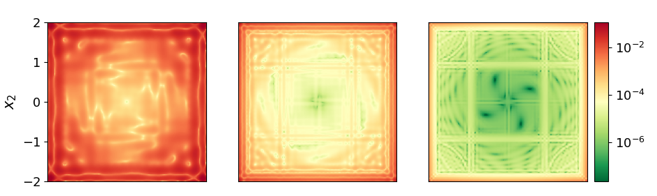
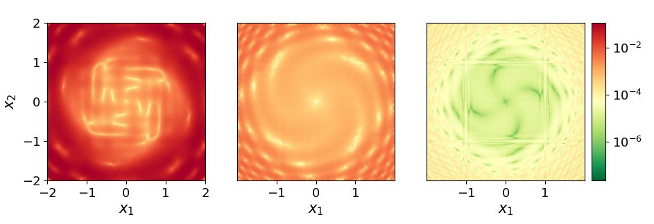
Figure 1. Approximation error $\|\widehat{F}(x)-F(x)\|_{2}$ for system Equation 21 with $d\in\{441,1681,6561\}$ data points for a uniform (mesh sizes $\delta\in\{0.2,0.1,0.05\}$; top) and a Chebychev-based grid (bottom).

These also effect the maximum errors $\max\limits_{x\in\mathcal{X}_{\text{val}}}\|\widehat{F}(x)-F(x)\|_{2}$ that are depicted for the different numbers of data points $d$ and validation areas in Table 1. The closer we get to the origin of the domain, the smaller the maximal error, which indicates the proportional decrease proven in Corollary 2.8. It can also be seen that for smaller validation areas, i.e. the further afar the validation area is from the boundary, the better the surrogate model $\widehat{F}$ on the uniform grid performs in comparison to the Chebyshev-based grid. This is due to the construction of the Chebyshev-based grid that has a higher density of data points towards the boundary but therefore less data points close to the origin.

	$d=441$		$d=1681$		$d=6561$
	uniform	Chebyshev	uniform	Chebyshev	uniform	Chebyshev
$[-2.0,2.0]^{2}$	0.1205	0.1423	0.03770	0.00690	0.009540	0.000350
$[-1.0,1.0]^{2}$	0.0053	0.0222	0.00030	0.00111	0.000021	0.000064
$[-0.5,0.5]^{2}$	0.0007	0.0022	0.00004	0.00073	0.000001	0.000020

Table 1. Maximal error for one-step prediction of System Equation 21 using the kEDMD surrogate $\widehat{F}$ for uniform and Chebyshev-based grid on different snippets of the validation grid.

Next, we inspect regularized kEDMD with regularization parameter $\lambda=0.01$. In Figure 2, we again depict the one-step prediction errors $\|\widehat{F}_{\lambda}(x)-F(x)\|_{2}$ on $\Omega$ for the Chebyshev-based grid. The overall structure of the error is similar to what is depicted in Figure 1 without regularization. However, the closer we get to the origin, the error is increased by about two orders of magnitude compared to Figure 1. This is to be expected due to the additional term $\sqrt{\lambda}$ in the error estimate in Corollary 2.8.

Figure 2. Approximation error $\|\widehat{F}_{\lambda}(x)-F(x)\|_{2}$ for system Equation 21 with $d\in\{441,1681,6561\}$ data points for a Chebychev-based grid and regularization parameter $\lambda=0.01$.

For a long-term evaluation of the errors, we choose a uniform grid $\mathcal{X}=\delta\mathbb{Z}^{2}\cap\Omega$ with $\delta=0.2\cdot 2^{-3}=0.025$ to learn the surrogate dynamics $\widehat{F}_{\lambda}$ for the regularization parameters $\lambda=0$ and $\lambda=0.01$. For the two initial conditions $x^{0}_{1}=r(1,0)^{\top}$ and $x^{0}_{2}=r(\cos(\pi/4),\sin(\pi/4))^{\top}$ that are located on the circle centered at the origin with radius $r=1.9$ the one-step errors $\|\widehat{F}_{\lambda}(x(k;x^{0}_{j}))-F(x(k;x^{0}_{j}))\|_{2}$ for $k\in[0:20]$ and $j\in\{1,2\}$ are visualized in Figure 3 in the image on the left. The difference of the one-step errors decays along the asymptotically stable trajectory of the original dynamics, confirming the proportional error bound Corollary 3.8 and the asymptotic stability of the surrogate model Theorem 3.9.

Lastly, we validate the Lyapunov decrease condition Equation 15, i.e., $V(\widehat{F}(x))-V(x)+\alpha_{V}(\|x\|)\leq 0$, where the data-driven surrogate dynamics $\widehat{F}$ of Equation 21 are generated using the mesh size $\delta=0.05$. In the right plot of Figure 3, the value of $-(V(\widehat{F}(x))-V(x)+\alpha_{V}(\|x\|))$ for $x\in\mathcal{X}_{\text{val}}$ is plotted and we can observe that the decrease condition is in fact preserved as stated in Theorem 3.9.

Figure 3. Left: One-step error $\|\widehat{F}_{\lambda}(x(k;x^{0}_{j}))-F(x(k;x^{0}_{j}))\|_{2}$ along the trajectory of Equation 21 for $r=1.9$ and $\tilde{r}=0.95\sqrt{2}$ with different regularization parameters $\lambda$. Right: Visualization of the Lyapunov decrease $-(V(\widehat{F}(x))-V(x)+\alpha_{V}(\|x\|))$ for system Equation 21 with the kEDMD surrogate $\widehat{F}$.

4. Koopman approximants for control systems

In this section, we consider the discrete-time control-affine system

$$x^{+}=f(x,u)=g_{0}(x)+G(x)u,$$ (23)

where $x\in\Omega\subset\mathbb{R}^{n}$ and the control $u$ is contained in a bounded set $\mathbb{U}\subset\mathbb{R}^{m}$, $m\leq n$, with $\operatorname{span}\mathbb{U}=\mathbb{R}^{m}$. Here, we assume that the maps $g_{0}:\Omega\to\mathbb{R}^{n}$ and $G:\Omega\to\mathbb{R}^{n\times m}$ are locally Lipschitz continuous, i.e., there exist constants $L_{g}>0$ and $L_{G}>0$ such that

$$\|g_{0}(x)-g_{0}(y)\|\leq L_{g}\|x-y\|\qquad\text{and}\qquad\|G(x)-G(y)\|\leq L_{G}\|x-y\|$$

for all $x,y\in\Omega$. We furthermore assume that all entries of both $g_{0}$ and $G$ are functions in the RKHS $\mathbb{H}=\mathcal{N}_{\Phi_{n,k}}(\Omega)$ for some fixed $k\in\mathbb{N}$. Hereby, we note that, in view of Equation 3, $\mathcal{N}_{\Phi_{n,k_{1}}}(\Omega)\subset\mathcal{N}_{\Phi_{n,k_{2}}}(\Omega)$ for $k_{1}\geq k_{2}$.

Remark 4.1 (Continuous-time control-affine dynamics).

Often, systems Equation 23 are derived from continuous-time control-affine systems governed by the dynamics

$$\dot{x}(t):=\tilde{f}(x(t),u(t)):=\tilde{g}_{0}(x(t))+\sum_{i=1}^{m}u_{i}(t)\tilde{g}_{i}(x(t))$$ (24)

with locally Lipschitz-continuous maps $\tilde{g}_{i}:\Omega\rightarrow\mathbb{R}^{n}$, $i\in[0:m]$. Analogously to the autonomous case, see Remark 2.1, for a time step $\Delta t>0$ we obtain

$$x(\Delta t;\bar{x},u)=\bar{x}+\int_{0}^{\Delta t}\tilde{g}_{0}(x(s;\bar{x},u))\,\mathrm{d}s+\int_{0}^{\Delta t}\tilde{G}(x(s;\bar{x},u))u(s)\,\mathrm{d}s,$$

where $\tilde{G}$ is defined analogously to $G$ above – again tacitly assuming existence and uniqueness of the solution $x(\cdot;\bar{x},u)$ on $[0,\Delta t]$. Then, assuming that the control function $u$ is constant on the interval $(0,\Delta t)$, a Taylor-series expansion of the solution at $t=0$ yields

$$x(\Delta t;\bar{x},u)=\bar{x}+\Delta t\left[\tilde{g}_{0}(\bar{x})+\tilde{G}(\bar{x})u\right]+\mathcal{O}(\Delta t^{2}),$$

where we have invoked compactness of $\mathbb{U}$ and Lipschitz continuity of $f(\cdot,u)$ and $\frac{\partial}{\partial x}f(\cdot,u)$ on $\overline{\Omega}$. Hereby, we have identified the (constant) control functions with the respective control value $u\in\mathbb{U}\subset\mathbb{R}^{m}$. Thus, we obtain a discrete-time system Equation 23 up to an arbitrarily small error if the time step $\Delta t$ is sufficiently small. This is in alignment with the theory of sampled-data systems with zero-order hold, see, e.g., [29].

In this section, we propose a novel learning architecture to learn Koopman approximants of the control-affine system Equation 23, that allows for flexible sampling of state-control pairs $(\bar{x}_{i},\bar{u}_{i},\bar{x}_{i}^{+})$ with $\bar{x}_{i}\in\Omega$, $\bar{u}_{i}\in\mathbb{U}$, and $\bar{x}_{i}^{+}=f(\bar{x}_{i},\bar{u}_{i})$, $i\in[1:d]$. The result of our proposed kEDMD-based algorithm are control-affine surrogate dynamics

$$x^{+}=\widehat{f}(x,u)=\widehat{g}_{0}(x)+\widehat{G}(x)u$$ (25)

using regression and interpolation in Wendland native spaces. In Theorem 4.3, we prove a uniform bound on the approximation error $\|f(x,u)-\widehat{f}(x,u)\|$, similarly as in Corollary 2.8 for the approximants $\widehat{F}$ and $\widehat{F}_{\lambda}$ of the dynamical system Equation DS. Then, we provide an application of the derived proportional bound in view of feedback stabilization. To be more precise, we prove in Section 4.2 that if a feedback stabilizes the surrogate dynamics Equation 25, the desired set point is stabilized in the original system (and vice versa). Last, the established error bounds are validated numerically in Section 4.3.

4.1. Koopman approximants, flexible sampling, and error bounds

We propose a novel learning architecture to generate Koopman approximants for control-affine systems with the following two key features: On the one hand, the algorithm can be used with (almost) arbitrary state-control data allowing for highly flexible sampling including i.i.d., ergodic, and trajectory-based data generation. On the other hand, we rigorously show bounds on the full approximation error with explicit convergence rates in the infinite-data limit and, foremost, allow for controller design with closed-loop guarantees without imposing restrictive invariance assumptions on the dictionary in EDMD. To the best of our knowledge, this combination is, up to now, unique. We note that Koopman-based approximations of control-affine systems in an RKHS framework with flexible sampling were also presented in [3], where the kernel (and thus also the RKHS) is suitably extended to capture the control dependency. Therein, however, no error bounds were provided. In addition, our novel approach allows to counteract numerical ill-conditioning by decomposing the approximation process in two steps labeled as macro and micro level, see the following paragraph for details.

The proposed method provided in detail in Algorithm 1 consists of two steps. In a first step, we determine $d$ clusters of size $N\geq m+1$, where $m$ is the control dimension in Equation 23. Each cluster corresponds to a center $x_{\ell}\in\Omega$, $\ell\in[1:d]$, and its $N$ nearest neighbors. The chosen centers $x_{\ell}$, $\ell\in[1:d]$, determine the fill distance $h_{\mathcal{X}}$. Then, we use the data triples $(\bar{x}_{i},\bar{u}_{i},\bar{x}_{i}^{+})$ corresponding to the cluster centered at $x_{\ell}$ to approximate the function values $g_{0}(x_{\ell})$ and $G(x_{\ell})$ for each $\ell\in[1:d]$. In a second step, based on the approximated function values from the first step, we apply RKHS-based interpolation to approximate the entries in the vector- and matrix-valued functions $g_{0}$ and $G$ in the $\sup$-norm. We briefly highlight that the clustering step in particular alleviates the inherent ill-conditioning of kernel-based interpolation tasks, which manifests in the rapidly decaying eigenvalues of the kernel matrix $\mathbf{K}_{\mathcal{X}}$ [40, Theorem 4.16]. This feature may be seen in the estimate of the subsequent Remark 4.5 as the term including the inverse of the kernel matrix may be controlled by the cluster radius $\varepsilon$.

Algorithm 1 Data-based approximation of the controlled flow map

Input: Triples $(\bar{x}_{i},\bar{u}_{i},\bar{x}_{i}^{+})$, $i\in[1:\bar{d}]$, where $\bar{x}_{i}^{+}=f(\bar{x}_{i},\bar{u}_{i})$, $\bar{x}_{i}\in\Omega$, $\bar{u}_{i}\in\mathbb{U}$, $i\in[1:\bar{d}]$. Number of clusters $d\geq\lfloor\bar{d}/N\rfloor$ and minimal number of cluster elements $N\geq m+1$.

Output: Approximation $\widehat{f}$ as in Equation 25.

 

Initialisation: Define the set $\bar{\mathcal{X}}=\{\bar{x}_{i}:i\in[1:\bar{d}]\}$.

Step 1: Clustering. Choose $\mathcal{X}=\{x_{1},\ldots,x_{d}\}\subset\Omega$.
For each $\ell\in[1:d]$:
 $\bullet$ Choose $N$ nearest neighbors $\{x_{\ell,1},\ldots,x_{\ell,N}\}\subset\overline{\mathcal{X}}$ of $x_{\ell}$
 $\bullet$ For $j\in[1:N]$: set $u_{\ell,j}=\bar{u}_{i}$ if $x_{\ell,j}=\bar{x}_{i}$
 $\bullet$ Define

$$U_{\ell}:=\begin{bmatrix}1&\dots&1\\ u_{\ell,1}&\dots&u_{\ell,N}\end{bmatrix}.$$ (26)

$\bullet$ Approximate $g_{0}(x_{\ell})$ and $G(x_{\ell})$ by solving

$$H_{\ell}^{*}:=\operatorname*{arg\,min}_{[y\;\;\;Y]\in\mathbb{R}^{n\times m+1}}\Big{\|}\begin{bmatrix}x_{\ell,1}^{+}&\dots&x_{\ell,N}^{+}\end{bmatrix}-\begin{bmatrix}y&Y\end{bmatrix}U_{\ell}\Big{\|}_{F}.$$ (27)

Step 2: Interpolation. For $p\in[1:n]$ and $q\in[1:m+1]$, compute

$$\widehat{H}_{pq}:=((H^{*}_{\ell})_{pq})_{\ell\in[1:d]}^{\top}\mathbf{K}_{\mathcal{X}}^{-1}\mathbf{k}_{\mathcal{X}}.$$ (28)

Set $\begin{bmatrix}\widehat{g}_{0}&\widehat{G}\end{bmatrix}=\widehat{H}$ and define $\widehat{f}$ as in Equation 25.

We briefly comment on the algorithmic choices of Algorithm 1.

Remark 4.2 (Sampling and clustering).

In Algorithm 1, the points $x_{1},\ldots,x_{d}$ can be seen as points on a “macroscopic” scale whereas the triples $(x_{\ell,i},u_{\ell,i},x_{\ell,i}^{+})$, based on the nearest neighbors, could be understood as data on a “microscopic level”. For the sampling of the data triples $(\bar{x}_{i},\bar{u}_{i},\bar{x}_{i}^{+})$, $i\in[1:\bar{d}]$, and the clustering step in Algorithm 1, various strategies could be applied.

A natural choice for the centers $x_{\ell}$, $\ell\in[1:d]$, would be to minimize the fill distance $h_{\mathcal{X}}$ of the macro level $\mathcal{X}$. Clearly, this choice also influences the precision for the approximation step Equation 27, where we approximate the function values at $\mathcal{X}$ by measurements of the flow at the nearest neighbors. Both quantities, i.e., the fill distance $h_{\mathcal{X}}$ and the radii of the clusters with the $N$ nearest neighbors are reflected in the error bound of Theorem 4.3. For fixed $N$, these quantities may be rendered arbitrarily small, if a sufficiently fine resolution by the micro level data set $\overline{\mathcal{X}}$ is provided (e.g. by grid-based or i.i.d. sampling).

Next, we present the main result of this section which provides a bound on the full approximation error $\|f-\widehat{f}\|$. In its proof, we first estimate the approximation error made in Step 1 of Algorithm 1 and then incorporate this bound into an error analysis concerning the interpolation in Step 2.

Theorem 4.3.

Assume that $U_{\ell}\in\mathbb{R}^{(m+1)\times N}$ in Equation 26 has full rank $m+1$ for all $\ell\in[1:d]$. Then, there exist constants $C,h_{0}>0$ such that for any set $\mathcal{X}\subset\Omega$, chosen in Step 1 of Algorithm 1, with $h_{\mathcal{X}}<h_{0}$, the error between the controlled map $f$ and its surrogate $\widehat{f}$ constructed by Algorithm 1 satisfies, for any $(x,u)\in\Omega\times\mathbb{U}$:

$$\|f(x,u)-\widehat{f}(x,u)\|_{\infty}\leq CD(x)(1+\|u\|_{1})$$

where

$$D(x)=h_{\mathcal{X}}^{k-1/2} \operatorname{dist}(x,\mathcal{X})\max_{p,q}\|H_{pq}\|_{\mathbb{H}}$$

$$+\sqrt{2N}\big{(}\max_{\ell\in[1:d]}\|U_{\ell}^{\dagger}\|\big{)}(L_{g}+L_{G}R)\Phi_{n,k}^{1/2}(0)\big{(}\max_{v\in\mathbbm{1}}v^{\top}\mathbf{K}_{\mathcal{X}}^{-1}v\big{)}^{1/2}\varepsilon.$$

with the maximal cluster size $\varepsilon=\max_{(\ell,j)\in[1:d]\times[1:N]}\|x_{\ell,j}-x_{\ell}\|$, $H=\begin{bmatrix}g_{0}&G\end{bmatrix}$,

$$R=\max\{\|u\|_{\infty}:u\in\mathbb{U}\},\quad\text{and}\quad\mathbbm{1}=\{v\in\mathbb{R}^{d}:v_{i}\in\{\pm 1\}\}.$$

In the proof of Theorem 4.3, we make use of the following lemma.

Lemma 4.4.

Let $\alpha\in\mathbb{R}^{d}$ and $f=\alpha^{\top}\mathbf{k}_{\mathcal{X}}\in V_{\mathcal{X}}$. Then, for all $x\in\Omega$,

$$|f(x)|^{2}\,\leq\,\mathsf{k}(x,x)\cdot\alpha^{\top}\mathbf{K}_{\mathcal{X}}\alpha.$$

Proof.

As $f=\sum_{k=1}^{d}\alpha_{k}\phi_{x_{k}}$, we have

$$\|f\|_{\mathbb{H}}^{2}=\langle\sum_{k=1}^{d}\alpha_{k}\phi_{x_{k}},\sum_{\ell=1}^{d}\alpha_{\ell}\phi_{x_{\ell}}\rangle=\sum_{k,\ell=1}^{d}\alpha_{k}\alpha_{\ell}\cdot\mathsf{k}(x_{k},x_{\ell})=\alpha^{\top}\mathbf{K}_{\mathcal{X}}\alpha.$$

Therefore, the claim follows from $|f(x)|^{2}=|\langle f,\phi_{x}\rangle_{\mathbb{H}}|^{2}\leq\|\phi_{x}\|_{\mathbb{H}}^{2}\|f\|_{\mathbb{H}}^{2}$ and $\|\phi_{x}\|_{\mathbb{H}}^{2}=\langle\phi_{x},\phi_{x}\rangle=\phi_{x}(x)=\mathsf{k}(x,x)$. ∎

Proof of Theorem 4.3.

Let $\ell\in[1:d]$. First of all, we show that

$$|H_{pq}(x_{\ell})-(H_{\ell}^{*})_{pq}|\,\leq\,\sqrt{2N}(L_{g}+L_{G}R)\|U_{\ell}^{\dagger}\|\cdot\varepsilon_{\ell},$$ (29)

where $\varepsilon_{\ell}=\max_{j\in[1:N]}\|x_{\ell,j}-x_{\ell}\|$. For this, note that $H_{\ell}^{*}=X_{\ell}^{+}U_{\ell}^{\dagger}$, where $X_{\ell}^{+}:=\begin{bmatrix}x_{\ell,1}^{+}&\dots&x_{\ell,N}^{+}\end{bmatrix}$. Hence, indeed,

$$|H_{pq}(x_{\ell})-(H_{\ell}^{*})_{pq}|^{2} =\big{|}e_{p}^{\top}H(x_{\ell})U_{\ell}U_{\ell}^{\dagger}e_{q}-e_{p}^{\top}X_{\ell}^{+}U_{\ell}^{\dagger}e_{q}\big{|}^{2}$$

$$\leq\|e_{p}^{\top}H(x_{\ell})U_{\ell}-e_{p}^{\top}X_{\ell}^{+}\|^{2}\cdot\|U_{\ell}^{\dagger}e_{q}\|^{2}$$

$$\leq\|U_{\ell}^{\dagger}\|^{2}\sum\nolimits_{s=1}^{N}\Big{|}e_{p}^{\top}H(x_{\ell})Ue_{s}-e_{p}^{\top}X_{\ell}^{+}e_{s}\Big{|}^{2}$$

$$=\|U_{\ell}^{\dagger}\|^{2}\sum\nolimits_{s=1}^{N}\big{|}e_{p}^{\top}\begin{bmatrix}g(x_{\ell})-g(x_{\ell,s})&G(x_{\ell})-G(x_{\ell,s})\end{bmatrix}\begin{bmatrix}1\\ u_{\ell,s}\end{bmatrix}\big{|}^{2}$$

$$\leq 2\|U_{\ell}^{\dagger}\|^{2}\sum\nolimits_{s=1}^{N}\Big{(}\|g(x_{\ell})-g(x_{\ell,s})\|^{2}+\|[G(x_{\ell})-G(x_{\ell,s})]u_{\ell,s}\|^{2}\Big{)}$$

$$\leq 2\|U_{\ell}^{\dagger}\|^{2}N(L_{g}^{2}+L_{G}^{2}R^{2})\varepsilon_{\ell}^{2},$$

and Equation 29 follows. Next, for $x\in\Omega$, we have

$$\big{|}H_{pq}(x)-\widehat{H}_{pq}(x)\big{|}\leq\big{|}H_{pq}(x)-P_{\mathcal{X}}H_{pq}(x)\big{|}+\big{|}P_{\mathcal{X}}H_{pq}(x)-\widehat{H}_{pq}(x)\big{|}.$$

The first summand can be estimated by Theorem 3.7:

$$\big{|}H_{pq}(x)-P_{\mathcal{X}}H_{pq}(x)\big{|}\leq Ch_{\mathcal{X}}^{k-1/2}\operatorname{dist}(x,\mathcal{X})\|H_{pq}\|_{\mathbb{H}}.$$

For the second, we estimate

$$\big{|}P_{\mathcal{X}}H_{pq}(x)-\widehat{H}_{pq}(x)\big{|} =\big{|}\big{[}(H_{pq})_{\mathcal{X}}-[(H_{\ell}^{*})_{pq}]_{\ell=1}^{d}\big{]}^{\top}\mathbf{K}_{\mathcal{X}}^{-1}\mathbf{k}_{\mathcal{X}}(x)\big{|}$$

$$\leq\big{\|}(H_{pq})_{\mathcal{X}}-[(H_{\ell}^{*})_{pq}]_{\ell=1}^{d}\big{\|}_{\infty}\big{\|}\mathbf{K}_{\mathcal{X}}^{-1}\mathbf{k}_{\mathcal{X}}(x)\big{\|}_{1}$$

$$\leq\sqrt{2N}(L_{g}+L_{G}R)\big{(}\max_{\ell\in[1:d]}\|U_{\ell}^{\dagger}\|\big{)}\varepsilon\cdot\big{\|}\mathbf{K}_{\mathcal{X}}^{-1}\mathbf{k}_{\mathcal{X}}(x)\big{\|}_{1},$$

and it remains to bound $\|\mathbf{K}_{\mathcal{X}}^{-1}\mathbf{k}_{\mathcal{X}}(x)\|_{1}$. For this, fix $x\in\Omega$ and consider

$$\|\mathbf{K}_{\mathcal{X}}^{-1}\textbf{k}_{\mathcal{X}}(x)\|_{1}=\sum_{i=1}^{d}\underbrace{|e_{i}^{\top}\mathbf{K}_{\mathcal{X}}^{-1}\textbf{k}_{\mathcal{X}}(x)|}_{=\pm e_{i}^{\top}\mathbf{K}_{\mathcal{X}}^{-1}\textbf{k}_{\mathcal{X}}(x)}=\bigg{(}\sum_{i=1}^{d}(-1)^{\ell_{i}}e_{i}\bigg{)}^{\top}\mathbf{K}_{\mathcal{X}}^{-1}\textbf{k}_{\mathcal{X}}(x),$$

where $\ell_{i}\in\{0,1\}$ depends on $x$. Let $v_{x}=\sum_{i=1}^{d}(-1)^{\ell_{i}}e_{i}$ and set $h:=v_{x}^{\top}\mathbf{K}_{\mathcal{X}}^{-1}\textbf{k}_{\mathcal{X}}\in V_{\mathcal{X}}$. Then $h(x)=\|\mathbf{K}_{\mathcal{X}}^{-1}\textbf{k}_{\mathcal{X}}(x)\|_{1}$ for the fixed $x$, and thus, by Lemma 4.4, $\|\mathbf{K}_{\mathcal{X}}^{-1}\textbf{k}_{\mathcal{X}}(x)\|_{1}^{2}=h^{2}(x)\leq\mathsf{k}(x,x)\cdot v_{x}^{\top}\mathbf{K}_{\mathcal{X}}^{-1}v_{x}$. Hence, noting that for the Wendland kernels it holds that $\mathsf{k}(x,x)=\Phi_{n,k}(0)$, we may estimate $\|\mathbf{K}_{\mathcal{X}}^{-1}\mathbf{k}_{\mathcal{X}}(x)\|_{1}^{2}\leq\Phi_{n,k}(0)\cdot\big{(}\max_{v\in\mathbbm{1}}v^{\top}\mathbf{K}_{\mathcal{X}}^{-1}v\big{)}$, which shows $\big{|}H_{pq}(x)-\widehat{H}_{pq}(x)\big{|}\leq C\cdot D_{pq}(x)$ with

$$D_{pq}(x)=h_{\mathcal{X}}^{k-1/2} \operatorname{dist}(x,\mathcal{X})\|H_{pq}\|_{\mathbb{H}}$$

$$+\sqrt{2N}(L_{g}+L_{G}R)\Phi_{n,k}^{1/2}(0)\big{(}\max_{\ell\in[1:d]}\|U_{\ell}^{\dagger}\|\big{)}\big{(}\max_{v\in\mathbbm{1}}v^{\top}\mathbf{K}_{\mathcal{X}}^{-1}v\big{)}^{1/2}\varepsilon.$$

Finally, for $x\in\Omega$ and $u\in\mathbb{U}$ this gives

$$\|f(x,u)-\widehat{f}(x,u)\|_{\infty}\leq\|g_{0}(x)-\widehat{g}_{0}(x)\|_{\infty}+\|[G(x)-\widehat{G}(x)]u\|_{\infty}$$

$$\leq \max_{p}|H_{p,1}(x)-\widehat{H}_{p,1}(x)|+\max_{p}\big{|}\sum\nolimits_{q=2}^{m+1}\big{[}H_{pq}(x)-\widehat{H}_{pq}(x)]u_{q-1}\big{|}$$

$$\leq C\max_{p}D_{p,1}(x)+C\max_{p,q}D_{p,q}(x)\sum_{q=1}^{m}|u_{q}|\leq C\max_{p,q}D_{p,q}(x)(1+\|u\|_{1})$$

and the theorem is proved. ∎

Currently, the upper bound presented in Theorem 4.3 depends on $h_{\mathcal{X}}$, $N$ and $\varepsilon$. As indicated in Remark 4.2, for fixed $N$, more and more data points in the micro grid $\overline{\mathcal{X}}$ may be leveraged by using also a finer macro grid $\mathcal{X}$ (thus, decreasing $h_{\mathcal{X}}$) and decreasing the cluster radius $\varepsilon$, as more neighbors are contained in a smaller neighborhood.

We conclude this section by a remark concerning alternative control sampling schemes and the dependence of the error bound on the number cluster elements $N$.

Remark 4.5.

(a) If it is possible to sample the controlled flow map $f(x,u)$ at $(x_{\ell},u_{\ell,i})$, $\ell\in[1:d]$, $i\in[1:N]$, we can choose $x_{\ell,i}=x_{\ell}$ in Step 2 of Algorithm 1 and thus $\varepsilon=0$. Hence, we obtain the error bound

$$\|f(x,u)-\widehat{f}(x,u)\|_{\infty}\leq C\cdot h_{\mathcal{X}}^{k-1/2}\operatorname{dist}(x,\mathcal{X})\max_{p,q}\|H_{pq}\|_{\mathbb{H}}(1+\|u\|_{1}).$$

(b) Let us briefly discuss the behavior of the term $\sqrt{N}\|U_{\ell}^{\dagger}\|$ in the estimate in Theorem 4.3 when the number of clusters $d$ remains constant and the cluster size $N$ grows. For this, we let $v_{i}:=\left[\begin{smallmatrix}1\\ u_{\ell,i}\end{smallmatrix}\right]\in\mathbb{R}^{m+1}$, $S:=\sum_{s=1}^{N}v_{i}v_{i}^{\top}$, and observe that $U_{\ell}U_{\ell}^{\top}=S$ and $U_{\ell}^{\dagger}=U_{\ell}^{\top}S^{-1}$. Therefore $\|U_{\ell}^{\dagger}\|^{2}=\|(U_{\ell}^{\dagger})^{\top}U_{\ell}^{\dagger}\|=\|S^{-1}U_{\ell}U_{\ell}^{\top}S^{-1}\|=\|S^{-1}\|=\frac{1}{\lambda_{\min}(S)}$, where $\lambda_{\min}(S)$ denotes the smallest eigenvalue of $S$. Hence, we have $\sqrt{N}\|U_{\ell}^{\dagger}\|=\sqrt{N/\lambda_{\min}(S)}$, and [45, Theorem 5.1.1] shows that if the $\bar{u}_{i}$ are drawn independently and uniformly from $[-R,R]^{m}$ and $R\geq\sqrt{3}$, then

$$\mathbb{P}\big{(}\sqrt{N}\|U_{\ell}^{\dagger}\|\geq c\big{)}\,\leq\,(1+m)\exp\big{(}-(1-\tfrac{1}{c})^{2}\cdot\tfrac{N}{1+R^{2}}\big{)},$$

hence it is exponentially unlikely that $\sqrt{N}\|U_{\ell}^{\dagger}\|$ is large if $N$ is large.

4.2. Feedback laws for stabilization

Finally, we consider stabilizing feedback laws for the original control-affine system Equation 23 and its surrogate Equation 25, where $\widehat{f}$ is defined via Algorithm 1. As it turns out, under certain assumptions, a stabilizing feedback for Equation 25 is also stabilizing for Equation 23.

Proposition 4.6.

Assume that the entries of $H=[g_{0}\;\;G]$ are contained in $\mathbb{H}$. Further, assume that there is a feedback law $\kappa:\Omega\to\mathbb{R}^{n}$, bounded on bounded sets such that $\widehat{F}_{\mathrm{cl}}(x):=\widehat{f}(x,\kappa(x))$ is asymptotically stable towards an equilibrium $x^{*}\in\Omega$ with $x^{*}\in\mathcal{X}$ with a Lyapunov function $V$ having a modulus of continuity $\omega_{V}$. Then $x^{*}$ is practically asymptotically stable w.r.t. $f(\cdot,\kappa(\cdot))=:F_{\rm cl}$, and the practical region decreases with decreasing fill distance $h_{\mathcal{X}}$ of the macro grid $\mathcal{X}$ and cluster size $\varepsilon$.

If further the samples are drawn in the sense of Remark 4.5(a) and if $\widehat{F}_{\mathrm{cl}}(x):=\widehat{f}(x,\kappa(x))$ is asymptotically stable towards $x^{*}\in\Omega$ with a Lyapunov function satisfying Assumption (a) or (b) of Theorem 3.9, then $\kappa$ also asymptotically stabilizes the original dynamics defined in Equation 23 towards $x^{*}$.

Proof.

We mimic the proofs of Theorem 3.5 and Theorem 3.9 for the closed loop system. In the first case, we observe that the error bound of Theorem 4.3 yields

$$\|F_{\mathrm{cl}}(x)-\widehat{F}_{\mathrm{cl}}(x)\| =\|f(x,\kappa(x))-\widehat{f}(x,\kappa(x))\|$$

$$\leq(c_{1}h_{\mathcal{X}}^{k-1/2}\operatorname{dist}(x,\mathcal{X})+c_{2}\varepsilon)(1+\|\kappa(x)\|_{1})\leq c_{3}(h_{\mathcal{X}}^{k+1/2}+\varepsilon)$$

where we invoked the boundedness of $\kappa$ and with constants $c_{1}:=C\max_{p,q}\|H_{pq}\|_{\mathbb{H}}$, $c_{2}:=C\sqrt{2N}(L_{g}+L_{G}R)\Phi_{n,k}^{1/2}(0)\big{(}\max_{\ell\in[1:d]}\|U_{\ell}^{\dagger}\|\big{)}\big{(}\max_{v\in\mathbbm{1}}v^{\top}\mathbf{K}_{\mathcal{X}}^{-1}v\big{)}^{1/2}$ and $c_{3}:=\max\{c_{1},c_{2}\}(1+\sup_{x\in\Omega}\|\kappa(x)\|_{1})$. This error bound is structurally the same as the bound of Corollary 2.8 with the cluster size $\varepsilon$ taking the role of $\sqrt{\lambda}$ and $\omega_{\Upsilon}=\operatorname{id}$. Thus, a similar argumentation as in the proof of Theorem 3.5 yields the claim.

To prove the second claim, we note that in view of the sampling of Remark 4.5(a), we may set $\varepsilon=0$ and obtain

$$\|F_{\mathrm{cl}}(x)-\widehat{F}_{\mathrm{cl}}(x)\| =\|f(x,\kappa(x))-\widehat{f}(x,\kappa(x))\|$$

$$\leq h_{\mathcal{X}}^{k-1/2}\|x-x^{*}\|\max_{p,q}\|H_{pq}\|_{\mathbb{H}}(1+\sup_{x\in\Omega}\|\kappa(x)\|_{1}),$$

where we used that $\operatorname{dist}(x,\mathcal{X})\leq\|x-x^{*}\|$ due to $x^{*}\in\mathcal{X}$. This inequality in particular implies that $x^{*}$ is also an equilibrium of ${F}_{\mathrm{cl}}(x)$. Further, the above is a proportional bound as in Corollary 3.8. Thus, an inspection of the proof of Theorem 3.9 shows that this implies also asymptotic stability of $F_{\mathrm{cl}}$. ∎

4.3. Numerics

Next, we illustrate the result of Theorem 4.3 by means of a numerical example. Therefore, consider the dynamics of the discretized Duffing oscillator given by

$$x^{+}=F(x,u)=x+\Delta t\begin{bmatrix}x_{2}\\ x_{1}-3x_{1}^{3}u\end{bmatrix}=\underbrace{\begin{bmatrix}{x}_{1}+\Delta tx_{2}\\ {x}_{2}+\Delta tx_{1}\end{bmatrix}}_{:=g_{0}(x)}+\underbrace{\begin{bmatrix}0\\ -\Delta t3x_{1}^{3}\end{bmatrix}}_{:=G(x)}u$$ (30)

with $\Delta t=0.05$ on $\Omega=[-2,2]^{2}$. As in Section 3.3, we use the coordinate functions $\psi_{i}(x)=x^{\top}e_{i}$, $i\in\{1,2\}$, as observables and for the Wendland radial basis functions, we choose the smoothness degree $k=1$. Further, whenever we refer to randomly drawn data samples, we always consider the uniform distribution on the respective set.

For the generation of the data points, we first use Chebyshev nodes to create the grid $\mathcal{X}\subset\Omega$ consisting of $d$ points that will act as the set of cluster points in the macro grid. With randomly chosen control values $u_{i}\in\mathbb{U}=[-2,2]$, the data triples $(x_{i},u_{i},x_{i}^{+})$ for $i\in[1:d]$ can be assembled.

To approximate the functions $g_{0}$ and $G$ at the grid points in $\mathcal{X}$ as presented in Step 1 of Algorithm 1, for a data point $x_{\ell}\in\mathcal{X}$ we choose the number of neighbors $N=25$ and then the neighbors $x_{\ell,i}$ for $i\in[1:N]$ are randomly drawn from a ball around $x_{\ell}$ with radius $\varepsilon=\frac{1}{d}$. For each $x_{\ell,i}$ a random $u_{\ell,i}\in\mathbb{U}$ is also drawn which yields the data points $(x_{\ell,i},u_{\ell,i},x^{+}_{\ell,i})$ for all $\ell\in[1:d]$ needed for the regression problem. Note that $\varepsilon$ is chosen to decease with an increasing number of cluster points. This is to make sure, that $\varepsilon$ can compensate the factor $\big{(}\max_{v\in\mathbbm{1}}v^{\top}\mathbf{K}_{\mathcal{X}}^{-1}v\big{)}^{1/2}$ in the error estimate in Theorem 4.3 in view of the decreasing smallest eigenvalue of $\mathbf{K}_{\mathcal{X}}$ when decreasing the fill distance of the macro grid $\mathcal{X}$, that is, increasing $d$.

For Step 2, the approximated values of $g_{0}$ and $G$ on the macro grid $\mathcal{X}$ from Step 1 are used for the interpolation as stated in Algorithm 1 to obtain the control-affine surrogate system $\widehat{F}$ in (30).

For the first simulation, we construct a kEDMD-based surrogate $\widehat{F}$ using a macro grid of $d=6561$ cluster points. Let $x(\cdot;x^{0},u)$ and $\widehat{x}(\cdot;x^{0},u)$ denote the flow from the initial value $x^{0}\in\Omega$ with control $u$ for the original model $F$ and surrogate $\widehat{F}$, respectively. In Figure 4, we inspect the difference of these trajectories for the initial condition $x^{0}=\binom{0.1}{0.1}$ and control sequences $\{u_{i}\}$ of length 50, where ten control values are randomly chosen from $\mathbb{U}$ and each of these control values is applied for five time steps (cf. Figure 4 on the right). In the phase space plot in the left of Figure 4, the two trajectories are barely distinguishable. When comparing the absolute error in the middle of Figure 4 on a log scale, we observe that the surrogate maintains an absolute error less than $10^{-4}$ for approximately 40 time steps (corresponding to the time $t=2$ in the continuous model).

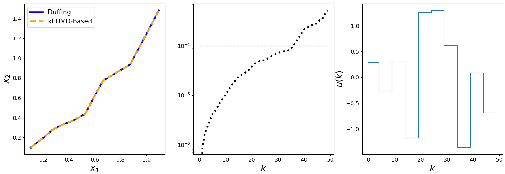
Figure 4. Trajectories $x(\cdot;x^{0},u)$ of system Equation 30 and its kEDMD surrogate $\widehat{x}(\cdot;x^{0},u)$ generated with Algorithm 1 (left) and their deviation $\|x(k;x^{0},u)-\widehat{x}(k;x^{0},u)\|_{2}$, $k\in[1:50]$, in norm (middle) for initial value $x^{0}=(0.1,0.1)^{\top}$ for the control sequence $u$ (right).

Next, we randomly chose 20 initial values $\hat{x}_{i}$ in $[-0.5,0.5]^{2}\subset\Omega$, as well as 20 random input sequences $\{u_{i}\}\subset[-0.1,0.1]\subset\Omega$ of length 30. These smaller boxes ensure that the trajectories remain in the domain $\Omega$.

In Figure 5 we depict statistical information on the error. The areas between maximum and median of the errors for the different numbers of cluster points $d$ barely overlap, that is, the reduction of the errors in the number of macro points $d$ is well noticeable. For $d=441$ the maximal error exceeds the $10^{-1}$ threshold nearly immediately after a few time steps and even the median transcends this bound at about 15 time steps are conducted. The greater $d$ is selected, the smaller the errors turn out.

Figure 5. Median and maximum of error of the kEDMD-based surrogate model Equation 25 to the real model Equation 30 from 20 trajectories for $d=1681$ cluster points. In between the median and maximum of the errors, the $0.8,0.9,0.95$-quantiles are plotted (left). Median and maximum for $d=441,1681,6561$ cluster points in one plot (right).

Finally, in Figure 6, we inspect the error of a one-step prediction in the Euclidean norm, similar to Figure 1 in Section 3.3. The learning of the kEDMD-based system is again performed for the three numbers of cluster points $d=441,1681,6561$ for the Chebyshev-based macro grid and $N=25$ data points in a neighborhood of $\varepsilon=\frac{1}{d}$. The errors $\max_{j\in[1:20]}\|F(x,u_{j})-\widehat{F}(x,u_{j})\|$ on a respective validation grid in $[-1,1]^{2}$ are computed for the control values in $\{-2+0.2(j-1)|\ j\in[1:20]\}$. In the intensity plots of Figure 6, it can be observed that the error evenly decreases the greater $d$ is chosen. This validates our results from Theorem 4.3: There are two sources of error that can be influenced, i.e., the fill distance of the macro grid $h_{\mathcal{X}}$ depending on number of cluster points $d$ and the maximal cluster size $\varepsilon$. If $\varepsilon$ is small enough to compensate the factor $\big{(}\max_{v\in\mathbbm{1}}v^{\top}\mathbf{K}_{\mathcal{X}}^{-1}v\big{)}^{1/2}$ that increases with $d$, the decrease of the fill distance by refining $\mathcal{X}$ yields a decay of the approximation error.

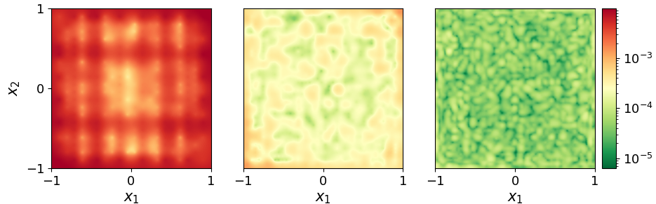
Figure 6. Approximation error $\max_{j\in[1:20]}\|F(x,u_{j})-\widehat{F}(x,u_{j})\|$ for the predicted system Equation 30 with $d\in\{441,1681,6561\}$ cluster points using a Chebychev-based grid (from left to right).

5. Conclusions and outlook

In this work, we provided a novel kernel EDMD scheme with flexible state-control sampling and uniform error estimates for data-driven modeling of dynamical (control) systems with stability guarantees.

In the first part of this work, we extended existing uniform bounds [20] on the full approximation error on Koopman approximants generated with kernel EDMD to Tychonov-regularized ones and derived proportional error bounds. While the first is important for robustness in view of the poor conditioning of kernel matrices (e.g. for noisy data), the second is key to show that asymptotic stability of an equilibrium w.r.t. the surrogate dynamics, certified by a Lyapunov function, is preserved for the original dynamical system and vice versa.

In the second part, we proposed a novel kernel-EDMD scheme for control-affine systems building upon arbitrarily-sampled control-state pairs and rigorously showed the first uniform (proportional) bounds on the full approximation error for control systems. We demonstrated that, as a consequence, stabilizing feedback laws designed for the data-driven surrogate models also ensure asymptotic stability w.r.t. the closed-loop of the original system building upon the proposed stability-analysis framework for kernel EDMD. We accompanied our findings by various numerical simulations.

Future work will be devoted to data-driven controller design leveraging the proposed highly-flexible sampling regime in combination with the novel proportional bounds derived in a non-restrictive setting. Herein, results from [12] and [6] may be leveraged for robustification and direct data-driven controller design.

Appendix A Results for the alternative surrogate

In this part of the Appendix, we discuss the properties of the approximant $\widetilde{\mathcal{K}}=P_{\mathcal{X}}\mathcal{K}P_{\mathcal{X}}$ of the Koopman operator (cf. Remark 2.3), where $\mathcal{X}=\{x_{1},\ldots,x_{d}\}\subset\Omega$, and $P_{\mathcal{X}}$ is the orthogonal projection onto $V_{\mathcal{X}}=\operatorname{span}\{\phi_{x_{1}},\ldots,\phi_{x_{d}}\}$. More generally, for $\lambda\geq 0$, we consider the regularized approximant

$$\widetilde{\mathcal{K}}_{\lambda}:=R_{\mathcal{X}}^{\lambda}\mathcal{K}R_{\mathcal{X}}^{\lambda}.$$

As for most of Section 2, we assume that the RKHS $\mathbb{H}$ is invariant under the Koopman operator $\mathcal{K}$, i.e. $\mathcal{K}\mathbb{H}\subset\mathbb{H}$. First of all, the approximant $\widetilde{\mathcal{K}}_{\lambda}$ can be written as

$$\widetilde{\mathcal{K}}_{\lambda}f=f_{\mathcal{X}}^{\top}(\mathbf{K}_{\mathcal{X}}+\lambda I)^{-1}\mathbf{K}_{\mathcal{X},F(\mathcal{X})}(\mathbf{K}_{\mathcal{X}}+\lambda I)^{-1}\mathbf{k}_{\mathcal{X}}.$$

Since

$$F(x)=\Upsilon(\Psi(F(x)))=\Upsilon\big{(}\big{[}\mathcal{K}\psi_{1}(x),\ldots,\mathcal{K}\psi_{M}(x)\big{]}^{\top}\big{)},$$

we define another family of surrogate models for Equation DS by

$$x^{+}=\widetilde{F}_{\lambda}(x),$$ (31)

where

$$\widetilde{F}_{\lambda}(x) =\Upsilon\big{(}\big{[}\widetilde{\mathcal{K}}_{\lambda}\psi_{1}(x),\ldots,\widetilde{\mathcal{K}}_{\lambda}\psi_{M}(x)\big{]}^{\top}\big{)}$$

$$=\Upsilon\big{(}\Psi_{\mathcal{X}}^{\top}(\mathbf{K}_{\mathcal{X}}+\lambda I)^{-1}\mathbf{K}_{\mathcal{X},F(\mathcal{X})}(\mathbf{K}_{\mathcal{X}}+\lambda I)^{-1}\mathbf{k}_{\mathcal{X}}(x)\big{)}.$$

In what follows, we will prove analogues of the basic results in Section 2 and Section 3 involving the approximant $\widehat{\mathcal{K}}_{\lambda}$ and the associated surrogate Equation 10 for the alternative approximant $\widetilde{\mathcal{K}}_{\lambda}$ and the surrogate Equation 31, introduced above. It is then clear that our stability results in Section 3 hold with $\widehat{F}_{\lambda}$ replaced by $\widetilde{F}_{\lambda}$.

A.1. Error bounds

The following theorem is the analogue of the combination of Theorem 2.4 and Corollary 2.8 for the alternative approximants.

Theorem A.1.

Let $k\geq 1$, $\lambda\geq 0$ and $F\in C_{b}^{\lceil\sigma_{n,k}\rceil}(\Omega;\mathbb{R}^{n})$. Then there are constants $C,h_{0}>0$ such that for any finite set $\mathcal{X}=\{x_{i}\}_{i=1}^{d}\subset\Omega$ of sample points with $h_{\mathcal{X}}\leq h_{0}$ and for all $\lambda\geq 0$, $f\in\mathcal{N}_{\Phi_{n,k}}(\Omega)$ and $x\in\Omega$ we have

$$|(\mathcal{K}f)(x)-(\widetilde{\mathcal{K}}_{\lambda}f)(x)|\leq C\big{(}h_{\mathcal{X}}^{k+1/2}+\sqrt{\lambda}\big{)}\|f\|_{\mathcal{N}_{\Phi_{n,k}}(\Omega)}.$$

In particular,

$$\|F(x)-\widetilde{F}_{\lambda}(x)\|\leq\omega_{\Upsilon}\Big{(}C\big{(}h_{\mathcal{X}}^{k+1/2}+\sqrt{\lambda}\big{)}\|\Psi\|_{\mathcal{N}^{l}_{\Phi_{n,k}}(\Omega)}\Big{)}\qquad\forall x\in\Omega$$

Proof.

The first claim on the error between $\mathcal{K}$ and $\widetilde{\mathcal{K}}_{\lambda}$ follows by a combination of [20, Theorem 5.2] and Lemma 2.5. The proof of the second claim on $F-\widetilde{F}_{\lambda}$ is very similar to that of Corollary 2.8. ∎

The next theorem improves the statement of Theorem A.1 towards proportional bounds, similarly as Theorem 3.7 and Corollary 3.8 did for the approximant $\widehat{\mathcal{K}}$.

Theorem A.2 (Proportional error bounds).

Assume that $k\geq 1+\frac{(-1)^{n}+1}{2}$ and $F\in C_{b}^{\lceil\sigma_{n,k}\rceil}(\Omega;\mathbb{R}^{n})$. Then there exist $C,h_{0}>0$ such that, for any finite set $\mathcal{X}=\{x_{i}\}_{i=1}^{d}\subset\Omega$ of sample points with $h_{\mathcal{X}}\leq h_{0}$ and all $f\in\mathcal{N}_{\Phi_{n,k}}(\Omega)$ and $x\in\Omega$ we have

$$|(\mathcal{K}f)(x)-(\widetilde{\mathcal{K}}f)(x)|\leq Ch_{\mathcal{X}}^{k-1/2}\max\{\operatorname{dist}(x,\mathcal{X}),\operatorname{dist}(F(x),\mathcal{X})\}\|f\|_{\mathcal{N}_{\Phi_{n,k}}(\Omega)}.$$

In particular,

$$\|F(x)-\widetilde{F}(x)\|\leq\omega_{\Upsilon}\big{(}Ch_{\mathcal{X}}^{k-1/2}\|\Psi\|_{\mathcal{N}_{\Phi_{n,k}}(\Omega)^{M}}\max\{\operatorname{dist}(x,\mathcal{X}),\,\operatorname{dist}(F(x),\mathcal{X})\}\big{)}.$$

Moreover, if $x^{*}\in\mathcal{X}$ is an equilibrium of the dynamics Equation DS, then

$$\|F(x)-\widetilde{F}(x)\|\leq\omega_{\Upsilon}\big{(}Ch_{\mathcal{X}}^{k-1/2}\|\Psi\|_{\mathcal{N}_{\Phi_{n,k}}(\Omega)^{M}}\|x-x^{*}\|\big{)}.$$

Proof.

We may use Theorem 3.7 to estimate

$$|(\mathcal{K}f)(x)-(\widetilde{\mathcal{K}}f)(x)| \leq|(\mathcal{K}f)(x)-(\mathcal{K}P_{\mathcal{X}}f)(x)|+|(\mathcal{K}P_{\mathcal{X}}f)(x)-(P_{\mathcal{X}}\mathcal{K}P_{\mathcal{X}}f)(x)|$$

$$=|[\mathcal{K}(I-P_{\mathcal{X}})f](x)|+|[(I-P_{\mathcal{X}})\mathcal{K}P_{\mathcal{X}}f](x)|$$

$$\leq|[(I-P_{\mathcal{X}})f](F(x))|+Ch_{\mathcal{X}}^{k-1/2}\operatorname{dist}(x,\mathcal{X})\|\mathcal{K}P_{\mathcal{X}}f\|_{\mathcal{N}_{\Phi_{n,k}}}$$

$$\leq Ch_{\mathcal{X}}^{k-1/2}\!\Big{[}\!\operatorname{dist}(F(x),\mathcal{X})\!+\!\operatorname{dist}(x,\mathcal{X})\|\mathcal{K}\|_{\mathcal{N}_{\Phi_{n,k}}\to\mathcal{N}_{\Phi_{n,k}}}\!\Big{]}\|f\|_{\mathcal{N}_{\Phi_{n,k}}},$$

which proves the main statement. The first claim of the “in particular”-part is now clear, the second follows from $\operatorname{dist}(x,\mathcal{X})\leq\|x-x^{*}\|$ and

$$\operatorname{dist}(F(x),\mathcal{X})\leq\|F(x)-x^{*}\|=\|F(x)-F(x^{*})\|\leq\|F\|_{C_{b}^{1}(\Omega,\mathbb{R}^{n})}\|x-x^{*}\|.$$

Hence, the theorem is proved. ∎

A.2. Equilibria

Let us compare the equilibria in the data set $\mathcal{X}$ of the dynamics Equation DS and the surrogate Equation 31.

Lemma A.3.

If $x^{*}\in\mathcal{X}$ is an equilibrium of Equation DS, then for each $f\in\mathbb{H}$ we have

$$(\widetilde{\mathcal{K}}f)(x^{*})=(\mathcal{K}f)(x^{*})=f(x^{*}).$$

In particular, $x^{*}$ is an equilibrium of Equation 31.

Proof.

Let $x^{*}=x_{k}$, and let $f\in\mathbb{H}$ be arbitrary. Clearly, $(\mathcal{K}f)(x_{k})=f(F(x_{k}))=f(x_{k})$. Note that $P_{\mathcal{X}}h$ for $h\in\mathbb{H}$ is the unique function in $V_{\mathcal{X}}$ which satisfies $(P_{\mathcal{X}}h)(x)=h(x)$ for all $x\in\mathcal{X}$. Hence, if we set $g=\mathcal{K}P_{\mathcal{X}}f$, then $(P_{\mathcal{X}}g)(x_{k})=g(x_{k})$ as $g\in\mathbb{H}$ and $x_{k}\in\mathcal{X}$. Therefore,

$$(\widetilde{\mathcal{K}}f)(x_{k})\!=\!(P_{\mathcal{X}}g)(x_{k})\!=\!g(x_{k})\!=\!(\mathcal{K}P_{\mathcal{X}}f)(x_{k})\!=\!(P_{\mathcal{X}}f)(F(x_{k}))\!=\!(P_{\mathcal{X}}f)(x_{k})=f(x_{k}),$$

which proves the lemma. ∎

The next proposition characterizes the equilibria in the data set $\mathcal{X}$ of Equation DS and the surrogate Equation 31.

Proposition A.4.

Let $x^{*}=x_{k}\in\mathcal{X}$. Then the following hold:

1. If $\Psi_{\mathcal{X}}^{\top}(I-\mathbf{K}_{\mathcal{X}}^{-1}\mathbf{K}_{\mathcal{X},F(\mathcal{X})})e_{k}=0$, then $x^{*}$ is an equilibrium of Equation 31. The converse is true if $\Upsilon:\mathbb{R}^{M}\to\mathbb{R}^{n}$ is injective.

2. If $x^{*}$ is an equilibrium of Equation DS, then $(I-\mathbf{K}_{\mathcal{X}}^{-1}\mathbf{K}_{\mathcal{X},F(\mathcal{X})})e_{k}=0$. The converse holds for kernels $\mathsf{k}$ with constant diagonal, in particular for the Wendland kernels.

Proof.

(i). We have

$$\widetilde{F}(x_{k})=\Upsilon\big{(}\Psi_{\mathcal{X}}^{\top}\mathbf{K}_{\mathcal{X}}^{-1}\mathbf{K}_{\mathcal{X},F(\mathcal{X})}\mathbf{K}_{\mathcal{X}}^{-1}\mathbf{k}_{\mathcal{X}}(x_{k})\big{)}=\Upsilon\big{(}\Psi_{\mathcal{X}}^{\top}\mathbf{K}_{\mathcal{X}}^{-1}\mathbf{K}_{\mathcal{X},F(\mathcal{X})}e_{k}\big{)}$$

Hence, if $\Psi_{\mathcal{X}}^{\top}(I-\mathbf{K}_{\mathcal{X}}^{-1}\mathbf{K}_{\mathcal{X},F(\mathcal{X})})e_{k}=0$, then

$$\widetilde{F}(x_{k})=\Upsilon\big{(}\Psi_{\mathcal{X}}^{\top}e_{k}\big{)}=\Upsilon(\Psi(x_{k}))=x_{k}.$$

Conversely, if $\widetilde{F}(x_{k})=x_{k}$, then

$$\Upsilon\big{(}\Psi_{\mathcal{X}}^{\top}\mathbf{K}_{\mathcal{X}}^{-1}\mathbf{K}_{\mathcal{X},F(\mathcal{X})}e_{k}\big{)}=x_{k}=\Upsilon(\Psi(x_{k})).$$

Hence, if $\Upsilon$ is injective, then $\Psi_{\mathcal{X}}^{\top}\mathbf{K}_{\mathcal{X}}^{-1}\mathbf{K}_{\mathcal{X},F(\mathcal{X})}e_{k}=\Psi(x_{k})=\Psi_{\mathcal{X}}^{\top}e_{k}$, which implies the claim.

(ii). Let $x^{*}=x_{k}$ be an equilibrium of Equation DS. Then

$$(I-\mathbf{K}_{\mathcal{X}}^{-1}\mathbf{K}_{\mathcal{X},F(\mathcal{X})})e_{k}=e_{k}-\mathbf{K}_{\mathcal{X}}^{-1}\mathbf{k}_{\mathcal{X}}(F(x_{k}))=e_{k}-\mathbf{K}_{\mathcal{X}}^{-1}\mathbf{k}_{\mathcal{X}}(x_{k})=e_{k}-\mathbf{K}_{\mathcal{X}}^{-1}\mathbf{K}_{\mathcal{X}}e_{k}=0.$$

Conversely, let $(I-\mathbf{K}_{\mathcal{X}}^{-1}\mathbf{K}_{\mathcal{X},F(\mathcal{X})})e_{k}=0$, and assume that $k(x,x)=c>0$ for all $x\in\Omega$. Then $(\mathbf{K}_{\mathcal{X}}-\mathbf{K}_{\mathcal{X},F(\mathcal{X})})e_{k}=0$, i.e.,

$$\mathbf{k}_{\mathcal{X}}(x^{*})=\mathbf{k}_{\mathcal{X}}(y^{*}),$$

where $y^{*}=F(x^{*})$. In particular, $\mathsf{k}(x^{*},y^{*})=\mathsf{k}(x^{*},x^{*})=c$. But this means that $|\langle\phi_{x^{*}},\phi_{y^{*}}\rangle|^{2}=c^{2}=\mathsf{k}(x^{*},x^{*})\mathsf{k}(y^{*},y^{*})=\|\phi_{x^{*}}\|^{2}\|\phi_{y^{*}}\|^{2}$. By Cauchy-Schwarz, $\phi_{x^{*}}$ and $\phi_{y^{*}}$ must be linearly dependent, which (by the strict positive definiteness of the kernel $\mathsf{k}$) implies $y^{*}=x^{*}$. ∎

Appendix B The regularization operator

Recall that the linear operator $R_{\mathcal{X}}^{\lambda}$ on $\mathbb{H}$ is defined by

$$R_{\mathcal{X}}^{\lambda}f=f_{\mathcal{X}}^{\top}(\mathbf{K}_{\mathcal{X}}+\lambda I)^{-1}\mathbf{k}_{\mathcal{X}}.$$

The following proposition is not used in the paper, but might be of independent interest.

Proposition B.1.

The following statements hold for the operator $R_{\mathcal{X}}^{\lambda}:\mathbb{H}\to\mathbb{H}$:

1. $(R_{\mathcal{X}}^{\lambda})^{*}=R_{\mathcal{X}}^{\lambda}\,\geq\,0$

2. $R_{\mathcal{X}}^{\lambda}P_{\mathcal{X}}=P_{\mathcal{X}}R_{\mathcal{X}}^{\lambda}=R_{\mathcal{X}}^{\lambda}$

3. $\|R_{\mathcal{X}}^{\lambda}f\|\leq\|P_{\mathcal{X}}f\|\leq\|f\|$ for $f\in\mathbb{H}$.

Proof.

(i). Let $f,g\in\mathbb{H}$. Then, with $\alpha=(\mathbf{K}_{\mathcal{X}}+\lambda I)^{-1}f_{\mathcal{X}}$ we have

$$\langle R_{\mathcal{X}}^{\lambda}f,g\rangle=\Big{\langle}\sum_{i=1}^{n}\alpha_{i}\phi(x_{i}),g\Big{\rangle}=\sum_{i=1}^{n}\alpha_{i}g(x_{i})=\alpha^{\top}g_{\mathcal{X}}=f_{\mathcal{X}}^{\top}(\mathbf{K}_{\mathcal{X}}+\lambda I)^{-1}g_{\mathcal{X}}.$$ (32)

Similarly, one shows that $\langle f,R_{\mathcal{X}}^{\lambda}g\rangle=f_{\mathcal{X}}^{\top}(\mathbf{K}_{\mathcal{X}}+\lambda I)^{-1}g_{\mathcal{X}}$. This shows $R_{\mathcal{X}}^{\lambda}=(R_{\mathcal{X}}^{\lambda})^{*}\,\geq\,0$.

(ii). $P_{\mathcal{X}}R_{\mathcal{X}}^{\lambda}=R_{\mathcal{X}}^{\lambda}$ follows from $\operatorname{ran}R_{\mathcal{X}}^{\lambda}\subset V_{\mathcal{X}}$ and $R_{\mathcal{X}}^{\lambda}P_{\mathcal{X}}=R_{\mathcal{X}}^{\lambda}$ from $R_{\mathcal{X}}^{\lambda}|_{V_{\mathcal{X}}^{\perp}}=0$. For the latter, note that $V_{\mathcal{X}}^{\perp}=\{f\in\mathbb{H}:f(x_{k})=0\,\forall k\in[1:d]\}$.

(iii). Let $g=R_{\mathcal{X}}^{\lambda}f$. Then $g_{\mathcal{X}}=\mathbf{K}_{\mathcal{X}}(\mathbf{K}_{\mathcal{X}}+\lambda)^{-1}f_{\mathcal{X}}$, and thus plugging $g$ into Equation 32 yields

$$\|R_{\mathcal{X}}^{\lambda}f\|^{2} =f_{\mathcal{X}}^{\top}(\mathbf{K}_{\mathcal{X}}+\lambda)^{-1}\mathbf{K}_{\mathcal{X}}(\mathbf{K}_{\mathcal{X}}+\lambda)^{-1}f_{\mathcal{X}}$$

$$=f_{\mathcal{X}}^{\top}\big{[}\underbrace{(\mathbf{K}_{\mathcal{X}}+\lambda)^{-1}\mathbf{K}_{\mathcal{X}}(\mathbf{K}_{\mathcal{X}}+\lambda I)^{-1}-\mathbf{K}_{\mathcal{X}}^{-1}}_{=:\mathbf{A}}\big{]}f_{\mathcal{X}}+f_{\mathcal{X}}^{\top}\mathbf{K}_{\mathcal{X}}^{-1}f_{\mathcal{X}}$$

$$=f_{\mathcal{X}}^{\top}\mathbf{A}f_{\mathcal{X}}+\|P_{\mathcal{X}}f\|^{2}.$$

By the spectral mapping theorem, the set of eigenvalues of $\mathbf{A}$ equals

$$\sigma(\mathbf{A})=\left\{\frac{\mu}{(\mu+\lambda)^{2}}-\frac{1}{\mu}:\mu\in\sigma(\mathbf{K}_{\mathcal{X}})\right\}=\left\{\frac{\mu^{2}-(\mu+\lambda)^{2}}{\mu(\mu+\lambda)^{2}}:\mu\in\sigma(\mathbf{K}_{\mathcal{X}})\right\}.$$

Hence, all eigenvalues of $\mathbf{A}$ are negative, which implies that $\mathbf{A}$ is negative definite. Therefore, $\|R_{\mathcal{X}}^{\lambda}f\|^{2}=f_{\mathcal{X}}^{\top}\mathbf{A}f_{\mathcal{X}}+\|P_{\mathcal{X}}f\|^{2}\leq\|P_{\mathcal{X}}f\|^{2}$. The second inequality $\|P_{\mathcal{X}}f\|\leq\|f\|$ is clear as $P_{\mathcal{X}}$ is an orthogonal projection. ∎

References

- [1] R. A. Adams and J. J. F. Fournier. Sobolev spaces, volume 140. Elsevier/Academic Press, Amsterdam, second edition, 2003.
- [2] J. Berberich, J. Köhler, M. A. Müller, and F. Allgöwer. Data-driven model predictive control with stability and robustness guarantees. IEEE Transactions on Automatic Control, 66(4):1702–1717, 2020.
- [3] P. Bevanda, B. Driessen, L. C. Iacob, R. Toth, S. Sosnowski, and S. Hirche. Nonparametric control-Koopman operator learning: Flexible and scalable models for prediction and control. Preprint arXiv:2405.07312, 2024.
- [4] L. Bold, L. Grüne, M. Schaller, and K. Worthmann. Data-driven MPC with stability guarantees using extended dynamic mode decomposition. IEEE Transactions on Automatic Control, 2024.
- [5] T. Breiten and B. Höveler. On the approximability of Koopman-based operator Lyapunov equations. SIAM Journal on Control and Optimization, 61(5):3131–3155, 2023.
- [6] F. Dörfler, J. Coulson, and I. Markovsky. Bridging direct and indirect data-driven control formulations via regularizations and relaxations. IEEE Transactions on Automatic Control, 68(2):883–897, 2022.
- [7] G. E. Fasshauer and Q. Ye. Reproducing kernels of generalized Sobolev spaces via a Green function approach with distributional operators. Numerische Mathematik, 119:585–611, 2011.
- [8] E. Gonzalez, M. Abudia, M. Jury, R. Kamalapurkar, and J. A. Rosenfeld. The kernel perspective on dynamic mode decomposition. Preprint arXiv:2106.00106, 2023.
- [9] D. Goswami and D. A. Paley. Bilinearization, reachability, and optimal control of control-affine nonlinear systems: A Koopman spectral approach. IEEE Transactions on Automatic Control, 67(6):2715–2728, 2021.
- [10] L. Grüne and J. Pannek. Nonlinear Model Predictive Control. Springer Int. Publishing, 2017.
- [11] W. M. Haddad and V. Chellaboina. Nonlinear dynamical systems and control: a Lyapunov-based approach. Princeton University Press, 2008.
- [12] L. Huang, J. Lygeros, and F. Dörfler. Robust and kernelized data-enabled predictive control for nonlinear systems. IEEE Transactions on Control Systems Technology, 2023.
- [13] L. C. Iacob, R. Tóth, and M. Schoukens. Koopman form of nonlinear systems with inputs. Automatica, 162, 2024.
- [14] C. M. Kellett. A compendium of comparison function results. Mathematics of Control, Signals, and Systems, 26:339–374, 2014.
- [15] S. Klus, F. Nüske, and B. Hamzi. Kernel-based approximation of the Koopman generator and Schrödinger operator. Entropy, 22(7), 2020.
- [16] M. Korda and I. Mezić. Linear predictors for nonlinear dynamical systems: Koopman operator meets model predictive control. Automatica, 93:149–160, 2018.
- [17] M. Korda and I. Mezić. On convergence of extended dynamic mode decomposition to the Koopman operator. Journal of Nonlinear Science, 28:687–710, 2018.
- [18] V. Kostic, P. Inzerili, K. Lounici, P. Novelli, and M. Pontil. Consistent long-term forecasting of ergodic dynamical systems. In 2024 Int. Conf. on Machine Learning, 2024.
- [19] V. Kostic, K. Lounici, P. Novelli, and M. Pontil. Sharp spectral rates for Koopman operator learning. Advances in Neural Information Processing Systems, 36, 2024.
- [20] F. Köhne, F. M. Philipp, M. Schaller, A. Schiela, and K. Worthmann. -error bounds for approximations of the Koopman operator by kernel extended dynamic mode decomposition. To appear in SIAM Journal of Applied Dynamical Systems, 2024. Preprint arXiv:2403.18809.
- [21] H. Li, S. Hafstein, and C. M. Kellett. Computation of Lyapunov functions for discrete-time systems using the Yoshizawa construction. In 53rd IEEE Conference on Decision and Control, pages 5512–5517, 2014.
- [22] E. T. Maddalena, P. Scharnhorst, Y. Jiang, and C. N. Jones. KPC: Learning-based model predictive control with deterministic guarantees. In Learning for Dynamics and Control, pages 1015–1026. PMLR, 2021.
- [23] I. Markovsky and F. Dörfler. Behavioral systems theory in data-driven analysis, signal processing, and control. Annual Reviews in Control, 52:42–64, 2021.
- [24] T. Martin, T. B. Schön, and F. Allgöwer. Guarantees for data-driven control of nonlinear systems using semidefinite programming: A survey. Annual Reviews in Control, 56, 2023.
- [25] A. Mauroy and I. Mezić. Global stability analysis using the eigenfunctions of the Koopman operator. IEEE Transactions on Automatic Control, 61(11):3356–3369, 2016.
- [26] A. Mauroy, Y. Susuki, and I. Mezić. Koopman operator in systems and control. Springer Nature, 2020.
- [27] I. Mezić. On numerical approximations of the Koopman operator. Mathematics, 10(7), 2022.
- [28] A. Narasingam and J. S.-I. Kwon. Koopman Lyapunov-based model predictive control of nonlinear chemical process systems. AIChE Journal, 65(11):e16743, 2019.
- [29] D. Nesić and A. R. Teel. Sampled-data control of nonlinear systems: an overview of recent results. Perspectives in robust control, pages 221–239, 2007.
- [30] F. Nüske, S. Peitz, F. Philipp, M. Schaller, and K. Worthmann. Finite-data error bounds for Koopman-based prediction and control. Journal of Nonlinear Science, 33, 2023.
- [31] S. E. Otto and C. W. Rowley. Koopman operators for estimation and control of dynamical systems. Annual Review of Control, Robotics, and Autonomous Systems, 4(1):59–87, 2021.
- [32] V. I. Paulsen and M. Raghupathi. An Introduction to the Theory of Reproducing Kernel Hilbert Spaces. Cambridge University Press, 2016.
- [33] S. Peitz, S. E. Otto, and C. W. Rowley. Data-driven model predictive control using interpolated Koopman generators. SIAM Journal on Applied Dynamical Systems, 19(3):2162–2193, 2020.
- [34] F. M. Philipp, M. Schaller, S. Boshoff, S. Peitz, F. Nüske, and K. Worthmann. Variance representations and convergence rates for data-driven approximations of Koopman operators. Preprint arXiv:2402.02494, 2024.
- [35] N. Powell, S. T. Paruchuri, A. Bouland, S. Niu, and A. Kurdila. Invariance and approximation of Koopman operators in native spaces. In American Control Conf. (ACC), pages 2871–2878, 2024.
- [36] K. Prag, M. Woolway, and T. Celik. Toward data-driven optimal control: A systematic review of the landscape. IEEE Access, 10:32190–32212, 2022.
- [37] J. L. Proctor, S. L. Brunton, and J. N. Kutz. Dynamic mode decomposition with control. SIAM Journal on Applied Dynamical Systems, 15(1):142–161, 2016.
- [38] J. L. Proctor, S. L. Brunton, and J. N. Kutz. Generalizing Koopman theory to allow for inputs and control. SIAM Journal on Applied Dynamical Systems, 17(1):909–930, 2018.
- [39] C. W. Rowley, I. Mezić, S. Bagheri, P. Schlatter, and D. S. Henningson. Spectral analysis of nonlinear flows. Journal of fluid mechanics, 641:115–127, 2009.
- [40] G. Santin. Approximation with kernel methods. Lecture notes. https://gabrielesantin.github.io/files/approximation_with_kernel_methods.pdf, 2018.
- [41] P. Scharnhorst, E. T. Maddalena, Y. Jiang, and C. N. Jones. Robust uncertainty bounds in reproducing kernel Hilbert spaces: A convex optimization approach. IEEE Transactions on Automatic Control, 68(5):2848–2861, 2022.
- [42] E. H. Spanier. Algebraic Topology. Springer-Verlag New York, Inc., 1966.
- [43] R. Strässer, M. Schaller, K. Worthmann, J. Berberich, and F. Allgöwer. Koopman-based feedback design with stability guarantees. IEEE Transactions on Automatic Control, 2024.
- [44] A. Surana. Koopman operator based observer synthesis for control-affine nonlinear systems. In 2016 IEEE 55th Conference on Decision and Control (CDC), pages 6492–6499, 2016.
- [45] J. A. Tropp. An introduction to matrix concentration inequalities. Foundations and Trends in Machine Learning, 8(1-2):1–230, 2015.
- [46] H. Wendland. Scattered data approximation, volume 17. Cambridge University Press, 2004.
- [47] H. Wendland and C. Rieger. Approximate interpolation with applications to selecting smoothing parameters. Numerische Mathematik, 101:729–748, 2005.
- [48] M. O. Williams, M. S. Hemati, S. T. Dawson, I. G. Kevrekidis, and C. W. Rowley. Extending data-driven Koopman analysis to actuated systems. IFAC-PapersOnLine, 49(18):704–709, 2016.
- [49] M. O. Williams, I. G. Kevrekidis, and C. W. Rowley. A data–driven approximation of the Koopman operator: Extending dynamic mode decomposition. Journal of Nonlinear Science, 25:1307–1346, 2015.
- [50] M. O. Williams, C. W. Rowley, and I. Kevrekidis. A kernel-based method for data-driven Koopman spectral analysis. Journal of Computational Dynamics, 2:247–265, 2015.
- [51] K. Worthmann, R. Strässer, M. Schaller, J. Berberich, and F. Allgöwer. Data-driven MPC with terminal conditions in the Koopman framework. In 63rd IEEE Conference on Decision and Control (CDC), 2024. To appear.
- [52] Y. Xu, Q. Wang, L. Mili, Z. Zheng, W. Gu, S. Lu, and Z. Wu. A data-driven Koopman approach for power system nonlinear dynamic observability analysis. IEEE Transactions on Power Systems, (2):4090–4104, 2024.
- [53] R. Yadav and A. Mauroy. Approximation of the Koopman operator via Bernstein polynomials. Preprint, arXiv:2403.02438, 2024.
- [54] C. Zhang and E. Zuazua. A quantitative analysis of Koopman operator methods for system identification and predictions. Comptes Rendus. Mécanique, 351(S1):1–31, 2023.
- [55] T. Zhao, M. Yue, and J. Wang. Deep-learning-based Koopman modeling for online control synthesis of nonlinear power system transient dynamics. IEEE Transactions on Industrial Informatics, 19(10):10444–10453, 2023.
- [56] M. Zhou, M. Lu, G. Hu, Z. Guo, and J. Guo. Koopman operator-based integrated guidance and control for strap-down high-speed missiles. IEEE Transactions on Control Systems Technology, 32(6):2436–2443, 2024.
- [57] V. Zinage and E. Bakolas. Neural Koopman Lyapunov control. Neurocomputing, 527:174–183, 2023.