IntComplex for high-order interactions

Abstract

Graphs serve as powerful tools for modeling pairwise interactions in diverse fields such as biology, material science, and social networks. However, they inherently overlook interactions involving more than two entities. Simplicial complexes and hypergraphs have emerged as prominent frameworks for modeling many-body interactions; nevertheless, they exhibit limitations in capturing specific high-order interactions, particularly those involving transitions from $n$-interactions to $m$-interactions. Addressing this gap, we propose IntComplex as an innovative framework to characterize such high-order interactions comprehensively. Our framework leverages homology theory to provide a quantitative representation of the topological structure inherent in such interactions. IntComplex is defined as a collection of interactions, each of which can be equivalently represented by a binary tree. Drawing inspiration from GLMY homology, we introduce homology for the detailed analysis of structural patterns formed by interactions across adjacent dimensions, $p$-layer homology to elucidate loop structures within $p$-interactions in specific dimensions, and multilayer homology to analyze loop structures of interactions across multiple dimensions. Furthermore, we introduce persistent homology through a filtration process and establish its stability to ensure robust quantitative analysis of these complex interactions. The proposed IntComplex framework establishes a foundational paradigm for the analysis of topological properties in high-order interactions, presenting significant potential to drive forward the advancements in the domain of complex network analysis.

1 Introduction

A graph is a collection of vertices and the edges connecting them. In the context of modeling and analyzing systems, vertices correspond to the entities within the system, such as atoms in a protein or individuals in a social network. The edges denote the interactions between these entities, such as covalent bonds between atoms or social relationships between individuals. Graph theory has been successfully utilized in various fields, including biology, material sciences, social network analysis and computer sciences [1, 2, 3, 4]. However, graphs implicitly ignore the high-order interactions since the edges only reflect the pairwise interactions.

Increasing evidence indicates that a single vertex can be influenced by multiple other vertices in a nonlinear manner, with such high-order interactions defying decomposition into simple pairwise interactions [5, 6, 7, 8] and the presence of high-order interactions may significantly impact the dynamics of the complex systems [9, 10, 11, 12]. Two prevalent frameworks for modeling these high-order interactions are simplicial complexes [13] and hypergraphs [14]. A simplicial complex extends the concept of a graph by incorporating triangles, tetrahedrons, and their higher-dimensional counterparts, whereas a hypergraph generalizes a simplicial complex by allowing the presence of missing faces. Notably, by integrating homology theory from algebraic topology, these high-order frameworks based models have achieved significant success in various aspects of drug design [15, 16, 17, 18], as well as in material design and discovery[19, 20, 21, 22].

However, there are still high-order interactions that simplicial complexes and hypergraphs cannot model. In both simplicial complex and hypergraph representations, an $n$-body interaction is represented by a set of $n$ vertices, meaning there are no internal structures within these $n$-interactions. In practice, it is common for a pairwise interaction from A to B to interact with C, akin to how the relationship between a father and mother in a family naturally affects their son. Figure 1 shows the difference among graphs, simplicial complexes, hypergraphs and IntComplexes (We propose in this work).

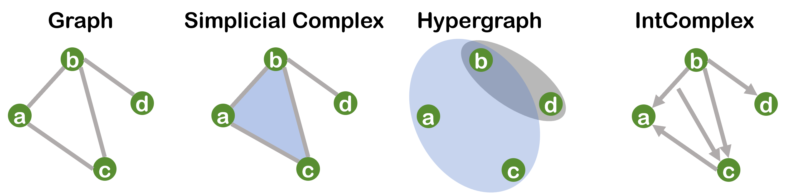
Figure 1: Comparison among a graph, simplicial complex, hypergraph and IntComplex. The simplicial complex and hypergraph can represent the high-order (3-order) interactions among a, b and c that cannot be captured in the graph representation. Specifically, the 3-order interaction among a, b and c are represented by a 2-simplex {a,b,c} and a 2-hyperedge {a,b,c} respectively. So the interaction from the interaction a and b to c cannot be captured in the simplicial complex and hypergraph but can be represented as a 3-interaction ((b, a), c) in the IntComplex.

As shown in Figure 1, the 3-interaction from the 2-interaction of b and a to c cannot be represented by the graph, simplicial complex and hypergraph but can be naturally modeled as a 3-interaction ((b, a), c) in the IntComplex. Consequently, simplicial complexes and hypergraphs are inadequate for modeling such high-order interactions. These high-order interactions are prevalent in various complex systems but have been explored in only a few studies[23, 24, 25] and remains an important research area [26]. And for the general high-order interaction from an $n$-interaction to an $m$-interaction, there is no mathematically well-defined modeling method as far as we know.

Here we present IntComplex for the modeling of high-order interactions, an IntComplex is a collection of interactions and the interaction from an $n$-interactoin to an $m$-interaction is modeled as an $(m+n)$-interaction. Further, we give the homology theory for analyzing the topological structures within the IntComplex, including the standard homology for the structures between adjacent-order interactions, $p$-layer homology for the loop structures within $p$-interactions, and multilayer homology for the loop structures among interactions of several orders. By considering a filtration of the IntComplex, we propose the persistent homology of IntComplex to give a multiscale quantitative characterization of the topological structures within the IntComplex, and give the stability theorem of the persistent homology to ensure its robustness. The paper is organized as follows: in section 2, we give the construction of IntComplexes and two representations of an interaction and its face operation, in section 3, we construct the homology theory of IntComplex and show that the homology is a simple homotopy invariant and a functor, in section 4, we give the persistent homology of IntComplexes and its stability, in section 5 , we give some experimental tests, a conclusion is in section 6.

2 IntComplex

In this section, we present the definition of IntComplex along with two different representations of the interactions and the face operation of the interactions.

2.1 Interaction and IntComplex

Definition 1 (Interaction of a set).

Given a set V, $\forall v\in V$ is called an 1-interaction of V. Take any $s$-interaction $\sigma_{s}$ and $t$-interaction $\sigma_{t}$ of V, the ordered pair $(\sigma_{s},\sigma_{t})$ is called an $(t+s)$-interaction of V $(t,s>0)$. Denote the set of all $p$-interactions of V by $Int_{p}(V)(p>0)$, $Int(V)=\bigcup_{p}Int_{p}(V)$.

From definition 1, $\forall\sigma_{p}\in Int_{p}(V)(p>1)$, there exists unique $\sigma_{i}\in Int_{i}(V),\sigma_{j}\in Int_{j}(V)(i+j=p)$ such that $\sigma_{p}=(\sigma_{i},\sigma_{j}).$ We call $\sigma_{i}$ and $\sigma_{j}$ the left daughter and right daughter of $\sigma_{p}$. We let the left and right daughters of any 1-interaction $\sigma_{1}$ be the empty set. Any interaction represents an interaction from its left daughter to its right daughter. For example, $\sigma_{p}=(\sigma_{i},\sigma_{j})$ represents an interaction from $\sigma_{i}$ to $\sigma_{j}$.

Definition 2 (IntComplex).

An IntComplex $\mathcal{I}$ over a set $V$ is a nonempty subcollection of $Int(V)$.

Denote the set of $p$-interactions of $\mathcal{I}$ by $\mathcal{I}_{p}$. We also call $\mathcal{I}_{p}$ the $p$-th layer of $\mathcal{I}$. The elements of $\mathcal{I}_{1}$ are called vertices of $\mathcal{I}$. Clearly, $\mathcal{I}_{1}$ is a subset of $V$, we remove from $V$ all the non-vertices so that $V=\mathcal{I}_{1}$. The IntComplex $\mathcal{I}^{\prime}$ is a subcomplex of the IntComplex $\mathcal{I}$ if $\mathcal{I}^{\prime}_{p}\subset\mathcal{I}_{p}(p\geqslant 1)$.

Example 1.

Figure 2 A shows an IntComplex $\mathcal{I}$ over $V=\{a,b,c,d\}$. $\mathcal{I}_{1}=\{a,b,c,d\}$, $\mathcal{I}_{2}=\{(b,a),(d,d)\}$, $\mathcal{I}_{3}=\{((b,a),c),(c,(d,d))\}$, $\mathcal{I}_{6}=\{(((b,a),c),(c,(d,d)))\}$, $\mathcal{I}_{p}=\emptyset(p\neq 1,2,3,6)$

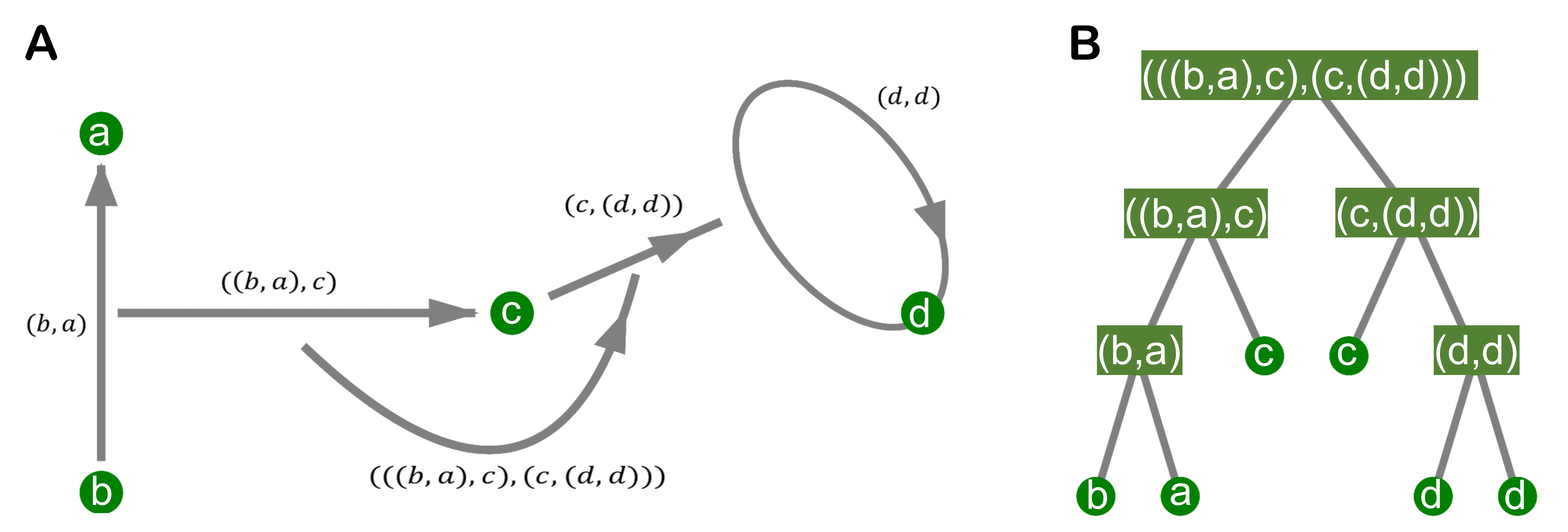
Figure 2: Illustration of the IntComplex and the binary tree representation of its interactions. A: An IntComplex over $V=\{a,b,c,d\}$. B: The binary tree representation of the interactions, every interaction $\sigma$ is represented by a binary tree whose root node is $\sigma$.

Example 2.

Given a directed graph $G$ with vertex set $V$ and edge set $E$. Let $\mathcal{I}_{1}=V,\mathcal{I}_{2}=E,\mathcal{I}_{p}=\emptyset(p>2)$, then $\mathcal{I}$ is an IntComplex. Hence any directed graph is a special IntComplex.

2.2 Interaction representation

2.2.1 Number Pair (NP) representation

Proposition 1.

Each n-interaction $\sigma_{n}\in Int_{n}(V)$ can be equivalently represented by a sequence of n ordered vertices $v_{1},v_{2},...,v_{n}$ and n-1 pairs of intergers $\{(l_{i},r_{i})|i=1,2,...,n-1\}$. And $\forall(l_{i_{1}},r_{i_{1}}),(l_{i_{2}},r_{i_{2}})$, they satisfy one of the followings

1. $[l_{i_{1}},r_{i_{1}}]\subsetneqq[l_{i_{2}},r_{i_{2}}]$ or $[l_{i_{2}},r_{i_{2}}]\subsetneqq[l_{i_{1}},r_{i_{1}}]$

2. $[l_{i_{1}},r_{i_{1}}]\cap[l_{i_{2}},r_{i_{2}}]=r_{i_{1}}=l_{i_{2}}$ or $[l_{i_{1}},r_{i_{1}}]\cap[l_{i_{2}},r_{i_{2}}]=l_{i_{1}}=r_{i_{2}}$ or $[l_{i_{1}},r_{i_{1}}]\cap[l_{i_{2}},r_{i_{2}}]=\emptyset$

Proof.

By induction, we can prove that each $n$-interaction $\sigma_{n}$ can be uniquely represented by a sequence of $n$ ordered vertices $v_{1},v_{2},...,v_{n}$ and $n$-1 round brackets “()”. These $n$ ordered vertices provide $n$+1 positions for the brackets to be put in. We number these positions by 1, 2,…, $n$+1 from left to right. Then each bracket “()” uniquely corresponds to a pair of numbers $(i,j)$ that are the positions of the bracket.

For the two properties of the number pairs. Each number pair corresponds to a bracket $``()"$, so the result follows by definition 1. ∎

We denote the $n$-interaction by $\sigma_{n}=[v_{1}...v_{n},\{(l_{i},r_{i})\}_{i=1}^{n-1}]$ and call it the NP representation of $\sigma_{n}$. The number pairs $\{(l_{i},r_{i})\}_{i=1}^{n-1}$ are positions of the $n-1$ brackets. For example, $[ba,\{(1,3)\}]$, $[dd,\{(1,3)\}]$, $[bac,\{(1,3),(1,4)\}]$, $[cdd,\{(2,4),(1,4)\}]$ and $[baccdd,\{(1,3),(1,4),(5,7),(4,7),(1,7)\}]$ are the NP representations of $(b,a)$, $(d,d)$, $((b,a),c)$, $(c,(d,d))$ and $(((b,a),c),(c,(d,d)))$ respectively.

Algorithm 1 Int2Tree

Input: an interaction $\sigma$ and the corresponding node $v$
  Output: the binary tree of $\sigma$

1:if $\sigma$ is an 1-interaction then

2:  return $v$

3:else

4:  $\sigma=(\sigma_{i},\sigma_{j})$

5:  add two nodes $v_{i},v_{j}$ as the left and right daughters of $v$

6:  return $T(v,{\rm Int2Tree}(\sigma_{i},v_{i}),{\rm Int2Tree}(\sigma_{j},v_{j}))$

Algorithm 2 Tree2Int

Input: a binary tree $bt$
  Output: the interaction of $bt$

1:if $bt$ has only one node $v$  then

2:  return $v$

3:else

4:  denote the left daughter and right daughter of $bt$ by $bt_{1}$ and $bt_{2}$ respectively.

5:  return ( Tree2Int($bt_{1}$), Tree2Int($bt_{2}$) )

2.2.2 Binary Tree (BT) representation

A binary tree is a tree in which each node has at most two daughter nodes. We denote a binary tree with $v$ as root node and $v_{i},v_{j}$ as the left and right daughters by $T(v,v_{i},v_{j})$. Each $n$-interaction $\sigma_{n}\in Int_{n}(V)$ can be represented as a binary tree by Algorithm 1. On the contrary, every binary tree $bt$ can be represented by an interaction by Algorithm 2. Let $T(\sigma_{n})=\rm Int2Tree(\sigma_{n})$, $S(bt)=\rm Tree2Int(bt)$.

Figure 2 B gives an example of the binary tree representation of the interactions in A. Each interaction $\sigma$ is represented by a binary tree whose root node is $\sigma$. For example, the 2-interaction $(b,a)$ is represented by the binary tree with two leaf nodes $b$ and $a$. The 3-interaction $(c,(d,d))$ is represented by the binary tree with three leaf nodes $c$, $d$ and $d$.

Proposition 2.

For any $n$-interaction $\sigma_{n}$, $\sigma_{n}=S(T(\sigma_{n}))$, for any binary tree $bt$, $bt=T(S(bt))$.

Proof.

Algorithm 1 and Algorithm 2 are inverse to each other. ∎

From proposition 2, we know each $n$-interaction has an equivalent NP representation containing $n$ vertices and $n-1$ pairs of position numbers, and an equivalent BT representation with $n$ leaf nodes. The binary tree representaiton can be derived by Algorithm 1. We call $T(\sigma_{n})$ the binary tree of $\sigma_{n}$.

2.3 Face

Given an interaction $\sigma$, consider its binary tree $T(\sigma)$, the $i$-th (from left to right) leaf node $v_{i}$ of $T(\sigma)$ has a minimal binary tree that contains $v_{i}$ as a daughter, denoted by $T_{i}$. Removing the $i$-th leaf node of $T(\sigma)$ is equivalent to repalce this subtree $T_{i}$ by the other daughter of $T_{i}$. In the NP representation, it is to remove the vertex $v_{i}$ and the number pair corrsponding to $T_{i}$.

Proposition 3.

Consider an $n$-interaction $\sigma_{n}=[v_{1}...v_{n},\{(l_{i},r_{i})\}_{i=1}^{n-1}]$. $\forall v_{p}(1\leqslant p\leqslant n)$, $\exists q$ such that $l_{q}\leqslant p<r_{q}$. Among such numbers q, there is a unique $q^{\prime}$ such that $r_{q^{\prime}}-l_{q^{\prime}}$ is the smallest one.

Proof.

The existance is obvious. For the uniqueness, suppose there are two number pairs $(l_{q_{1}},r_{q_{1}})$, $(l_{q_{2}},r_{q_{2}})$ such that $l_{q_{1}}\leqslant p<r_{q_{1}}$, $l_{q_{2}}\leqslant p<r_{q_{2}}$, then the interaction of these two pairs are not just one number, which contradicts with Proposition 1. ∎

We denote the number $q^{\prime}$ by $T(v_{i},\sigma_{n})=q^{\prime}$. The unique number pair of $v_{i}$ just corresponds to the minimal binary tree $T_{i}$ of $v_{i}$. Now we can give the face operation.

Definition 3 (Face).

Given an n-interaction $\sigma_{n}=[v_{1}...v_{n},\{(l_{i},r_{i})\}_{i=1}^{n-1}]$ over V, let $M_{\sigma_{n}}^{j}=\{(l_{i},r_{i})|1\leqslant i\leqslant n-1,i\neq T(v_{j},\sigma_{n})\}$. For each $(l_{t},r_{t})\in M^{j}_{\sigma_{n}}$, if $l_{t}>j$, replace $l_{t}$ by $l_{t}-1$, if $r_{t}>j$, replace $r_{t}$ by $r_{t}-1$. Perform this replacement for all elements of $M^{j}_{\sigma_{n}}$, denote the resulting set by $N^{j}_{\sigma_{n}}$. Then $[v_{1}...v_{j-1}v_{j+1}...v_{n},N_{\sigma_{n}}^{j}]$ is an $(n-1)$-interaction, define it as the $j$-th face of $\sigma_{n}$, denoted by $F_{j}(\sigma_{n})$. Given a binary tree T, define the $j$-th face of T to be the binary tree derived from T by removing the $j$-th leaf node, denoted by $F_{j}(T)$.

The $n$-interaction $\sigma_{n}$ has $n$ faces $\{F_{1}(\sigma_{n}),F_{2}(\sigma_{n}),...,F_{n}(\sigma_{n})\}$. The binary tree of $j$-th face of $\sigma_{n}$ is exactly the binary tree derived from $T(\sigma_{n})$ by removing the $j$-th leaf node. That is, $F_{j}(T(\sigma_{n}))=T(F_{j}(\sigma_{n})).$

Proposition 4.

$\forall i<j,F_{i}F_{j}=F_{j-1}F_{i}$.

Proof.

For any binary tree $bt$, $F_{i}F_{j}(bt)$ is the binary tree from $bt$ by first removing the $j$-th and then the $i$-th leaf nodes. $F_{j-1}F_{i}(bt)$ is the binary tree from $bt$ by first removing the $i$-th and then the $(j-1)$-th leaf nodes. Hence $F_{i}F_{j}(bt)=F_{j-1}F_{i}(bt)$.

$\forall\sigma_{n}\in Int_{n}(V)$, We have $F_{i}F_{j}(T(\sigma_{n}))=F_{j-1}F_{i}T(\sigma_{n})$, so $S(F_{i}F_{j}T(\sigma_{n}))=SF_{j-1}F_{i}T(\sigma_{n})$, $STF_{i}F_{j}(\sigma_{n})=STF_{j-1}F_{i}(\sigma_{n})$, that is, $F_{i}F_{j}=F_{j-1}F_{i}$. ∎

3 Homology of IntComplex

In this section, we introduce three types of homology groups for the IntComplex. First, we present homology for the structure composed of adjacent-layer interactions. Next, we describe layer-homology for structures formed by interactions within specific layers. Lastly, we discuss multilayer-homology for structures arising from interactions across multiple layers. Specifically, our focus lies on analyzing loop structures for layer-homology and multilayer-homology.

3.1 Boundary operator and Homology

Fix a field $\mathbb{F}$ as the coefficient. Given an IntComplex $\mathcal{I}$ over $V$, Let $\Lambda_{p}(\mathcal{I})$ be the $\mathbb{F}$-vector space spanned by $Int_{p}(V)(p>0)$.

Definition 4 (Boundary operator).

For the $n$-interaction $\sigma_{n}=[v_{1}...v_{n},\{(l_{i},r_{i})\}_{i=1}^{n-1}]\in Int_{n}(V)$, We define the boundary operator $\partial_{n}:\Lambda_{n}(\mathcal{I})\rightarrow\Lambda_{n-1}(\mathcal{I})$ as follows:

$$\partial_{n}(\sigma_{n})=\sum_{j=1}^{k}(-1)^{j+1}F_{j}(\sigma_{n})$$

That is,

$$\partial_{n}([v_{1}...v_{n},\{(l_{i},r_{i})\}_{i=1}^{n-1}])=\sum_{j=1}^{k}(-1)^{j+1}[v_{1}...v_{i-1}v_{i+1}...v_{n},N_{\sigma_{n}}^{j}]$$

Further, we define $\Lambda_{0}(\mathcal{I})=0$ and $\partial:\Lambda_{1}(\mathcal{I})\rightarrow\Lambda_{0}(\mathcal{I})$ to be zero. In the binary tree representation, we have

$$\partial_{n}(T(\sigma_{n}))=\sum_{j=1}^{n}(-1)^{j+1}T(F_{j}(\sigma_{n}))$$

where $T(F_{j}(\sigma_{n}))$ is derived by removing the $j$-th leaf node of $T(\sigma_{n})$. Figure 3 shows the binary tree representation of the boundary operator for $\partial((a,b),c)=((b),c)-((a),c)+(a,b)=(b,c)-(a,c)+(a,b)$

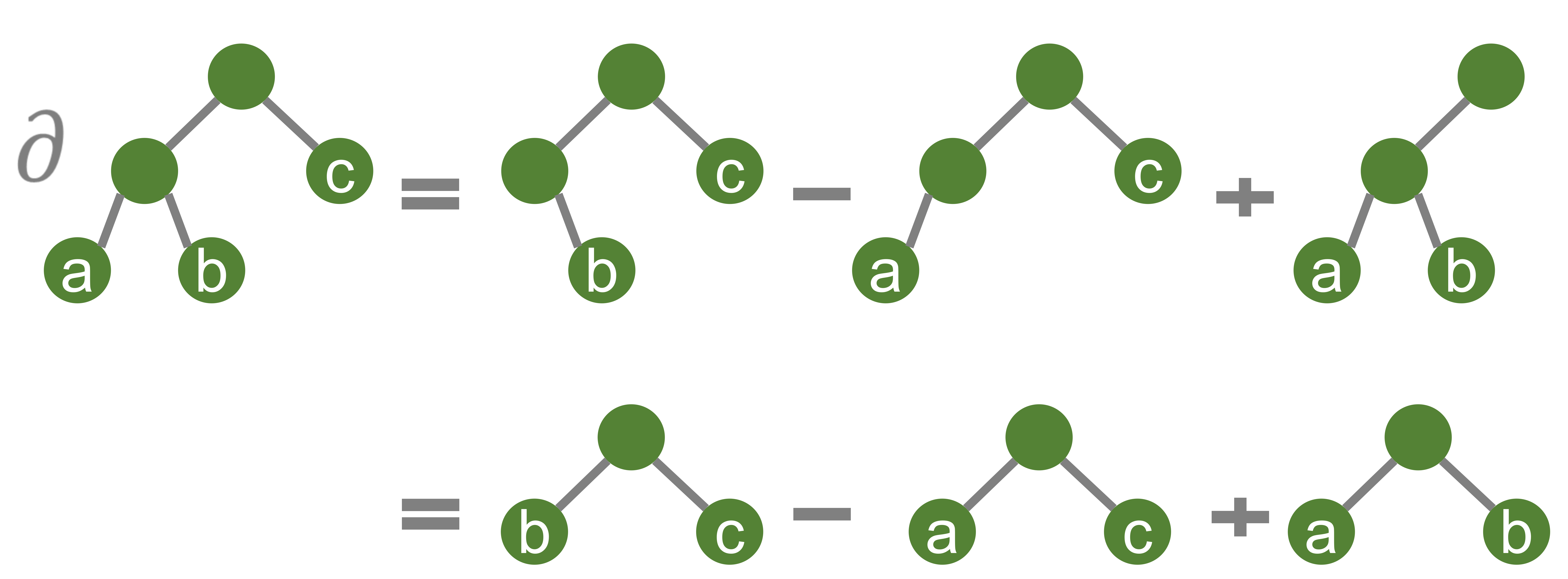
Figure 3: Illustration of the boundary operation bybinary tree.

Proposition 5.

$\partial\partial=0$

Proof.

$\forall\sigma_{n}\in Int_{n}(V)$,

$$\begin{split}\partial(\partial(\sigma_{n}))&=\partial(\sum_{i=1}^{n}(-1)^{i}F_{i}(\sigma_{n}))\\ &=\sum_{i=1}^{n}(-1)^{i}\partial(F_{i}(\sigma_{n}))\\ &=\sum_{i=1}^{n}(-1)^{i}\sum_{j=1}^{i-1}(-1)^{j+1}F_{j}(F_{i}(\sigma_{n}))+\sum_{i=1}^{n}(-1)^{i}\sum_{j=i+1}^{n}(-1)^{j}F_{j-1}(F_{i}(\sigma_{n}))\\ &=\sum_{1\leqslant j<i\leqslant n}(-1)^{i+j+1}F_{j}(F_{i}(\sigma_{n}))+\sum_{1\leqslant i<j\leqslant n}(-1)^{i+j}F_{j-1}(F_{i}(\sigma_{n}))\\ &=\sum_{1\leqslant i<j\leqslant n}(-1)^{i+j+1}F_{i}(F_{j}(\sigma_{n}))+\sum_{1\leqslant i<j\leqslant n}(-1)^{i+j}F_{j-1}(F_{i}(\sigma_{n}))~(shift~i~and~j~of~the~first~part)\\ &=\sum_{1\leqslant i<j\leqslant n}(-1)^{i+j+1}F_{i}(F_{j}(\sigma_{n}))-\sum_{1\leqslant i<j\leqslant n}(-1)^{i+j+1}F_{i}(F_{j}(\sigma_{n}))~(by~proposition~\ref{prop:11})\\ &=0\end{split}$$

∎

Consequently, we get a chain complex

$$...\rightarrow\Lambda_{p+1}(\mathcal{I})\xrightarrow{\partial}\Lambda_{p}(\mathcal{I})\xrightarrow{\partial}\Lambda_{p-1}(\mathcal{I})\xrightarrow{.}..\rightarrow\Lambda_{1}(\mathcal{I})\xrightarrow{0}\Lambda_{0}(\mathcal{I})=0$$

Denoted by $(\Lambda_{*}(\mathcal{I}),\partial_{*})$. Let $\mathcal{A}_{p}(\mathcal{I})$ be the $\mathbb{F}$-vector space spanned by $\mathcal{I}_{p}$, $\mathcal{A}_{p}(\mathcal{I})\subset\Lambda_{p}(\mathcal{I})$, but generally, $\partial(\mathcal{A}_{p}(\mathcal{I}))\not\subset\mathcal{A}_{p-1}(\mathcal{I})$. Considering the following subspace of $\mathcal{A}_{p}(\mathcal{I})$

$$\Omega_{p}(\mathcal{I})=\{\alpha_{p}\in\mathcal{A}_{p}(\mathcal{I})|\partial(\alpha_{p})\in\mathcal{A}_{p-1}(\mathcal{I})\}$$

We have $\partial(\Omega_{p}(\mathcal{I}))\subset\Omega_{p-1}(\mathcal{I})$, so we get a chain complex

$$...\rightarrow\Omega_{p+1}(\mathcal{I})\xrightarrow{\partial}\Omega_{p}(\mathcal{I})\xrightarrow{\partial}\Omega_{p-1}(\mathcal{I})\rightarrow...\rightarrow\Omega_{1}(\mathcal{I})\xrightarrow{0}0$$

Denoted by $(\Omega_{*}(\mathcal{I}),\partial_{*}(\mathcal{I}))$.

Definition 5 (Homology of IntComplex).

Define the p-th homology of the IntComplex $\mathcal{I}$ as the p-th homology of $(\Omega_{*}(\mathcal{I}),\partial_{*}(\mathcal{I}))$

$$H_{p}(\mathcal{I})=H_{p}(\Omega_{*}(\mathcal{I}),\partial_{*}(\mathcal{I}))=Ker\partial_{p}|_{\Omega_{*}(\mathcal{I})}/Im\partial_{p+1}|_{\Omega_{*}(\mathcal{I})}$$

Define the $p$-th betti number of $\mathcal{I}$ as the dimension of $H_{p}(\mathcal{I})$, denoted by $\beta_{p}=dim(H_{p}(\mathcal{I}))$.

3.2 Simple Homotopy type

Definition 6.

Given an IntComplex $\mathcal{I}$, a pair of interactions $(\sigma_{p},\tau_{p+1})$ is called free if $\sigma_{p}$ is a face of $\tau_{p+1}$ and not face of any other $(p+1)$-interactions.

Definition 7.

Given an IntComplex $\mathcal{I}$, assume $(\sigma,\tau)$ is a free pair of $\mathcal{I}$, $\mathcal{I}^{\prime}=\mathcal{I}\setminus\{\sigma,\tau\}$ is also an IntComplex. We call $\mathcal{I}^{\prime}$ is derived by an collapse from $\mathcal{I}$ and $\mathcal{I}$ is derived from $\mathcal{I}^{\prime}$ by an expansion.

Definition 8.

Given two IntComplexes $\mathcal{I}$ and $\mathcal{I}^{\prime}$, we say they have the same simple homotopy type if $\mathcal{I}$ can be derived from $\mathcal{I}^{\prime}$ by finite collapses and expansions.

Theorem 1.

If two IntComplexes $\mathcal{I}$ and $\mathcal{I}^{\prime}$ have the same simple homotopy type, then for any $p\geqslant 0$

$$H_{p}(\mathcal{I})\cong H_{p}(\mathcal{I}^{\prime})$$

Proof.

Assume $\mathcal{I}^{\prime}$ is derived from $\mathcal{I}$ by a collapse of the free pair $(\sigma_{n},\tau_{n+1})$ where $\sigma_{n}$ is an $n$-interaction and $\tau$ is an $(n+1)$-interaction. It suffices to prove that $H_{p}(\mathcal{I})\cong H_{p}(\mathcal{I}^{\prime})$. We have the chain complexes $(\Omega_{*}(\mathcal{I},\partial_{*}),(\Omega_{*}(\mathcal{I}^{\prime},\partial_{*})$ for $\mathcal{I}$ and $\mathcal{I}^{\prime}$ respectively. Note that $(\Omega_{*}(\mathcal{I}^{\prime}),\partial_{*})$ is a subchain complex of $(\Omega_{*}(\mathcal{I}),\partial_{*})$, so we have the quotient complex $(\Omega_{*}(\mathcal{I}/\mathcal{I}^{\prime}),\partial_{*})$ where

$$\Omega_{p}(\mathcal{I}/\mathcal{I}^{\prime})=\Omega_{p}(\mathcal{I})/\Omega_{p}(\mathcal{I}^{\prime})$$

and the exact sequence of chain complex

$$0\rightarrow\Omega_{*}(\mathcal{I}^{\prime})\xrightarrow{i}\Omega_{*}(\mathcal{I})\xrightarrow{j}\Omega_{*}(\mathcal{I}/\mathcal{I}^{\prime})\rightarrow 0$$

where $i$ is the subcomplex injection and $j$ is the quotient projection. Consequently, it suffices to prove the quotient complex $(\Omega_{*}(\mathcal{I}/\mathcal{I}^{\prime}),\partial_{*})$ is acyclic, that is, $H_{p}(\Omega_{*}(\mathcal{I}/\mathcal{I}^{\prime}))=0(p\geqslant 0)$.

1. if there not exists $\alpha\in\Omega_{n}(\mathcal{I})$ such that $\sigma_{n}\in\alpha$, $\tau_{n+1}\notin\Omega_{n+1}(\mathcal{I})$. In this case, $\Omega_{p}(\mathcal{I})=\Omega_{p}(\mathcal{I}^{\prime})(\forall p\geqslant 0)$, so $\Omega_{*}(\mathcal{I}/\mathcal{I}^{\prime})=0(\forall p\geqslant 0)$, it follows that the quotient complex is acyclic.

2. if there exists $\alpha\in\Omega_{n}(\mathcal{I})$ such that $\sigma_{n}\in\alpha$, there is $\gamma\in\Omega_{n+1}(\mathcal{I})$ such that $\tau_{n+1}\in\gamma$ and $\partial(\gamma)=\alpha$. In this case,

   $$\begin{cases}\Omega_{p}(\mathcal{I})=\Omega_{p}(\mathcal{I}^{\prime})&p<n\\ \Omega_{p}(\mathcal{I})=\Omega_{p}(\mathcal{I}^{\prime})\oplus<\alpha>&p=n\\ \Omega_{p}(\mathcal{I})=\Omega_{p}(\mathcal{I}^{\prime})\oplus<\gamma>&p=n+1\\ \Omega_{p}(\mathcal{I})=\Omega_{p}(\mathcal{I}^{\prime})&p>n+1\\ \end{cases}$$

   So the quotient complex has nonzero chain group only in dimension $n$ and $n+1$. We have the following quotient complex

   $$0\rightarrow<\gamma>\xrightarrow{\partial}<\alpha>\rightarrow 0$$

   $Ker\partial=0$, so $H_{n+1}(\Omega_{*}(\mathcal{I}/\mathcal{I}^{\prime}))=0$. $\partial(\gamma)=\alpha$, so $H_{n}(\mathcal{I}/\mathcal{I}^{\prime})=0$. It follows that he quotient complex is acyclic.

∎

3.3 Connected components and $H_{1}$

Given an IntComplex $\mathcal{I}$, a path of $\mathcal{I}$ is a sequence of vertices $v_{0},v_{1},...,v_{n}$ such that $(v_{i},v_{i+1})\in\mathcal{I}_{2}$ or $(v_{i+1},v_{i})\in\mathcal{I}_{2}$ for all $0\leqslant i<n$. Two vertices $u,v$ are called in the same connected component if there is a path connecting $u,v$. $\mathcal{I}$ is called connected if it only has one connected component.

Definition 9 (Disjoint union).

Given two IntComplexs $\mathcal{I}^{\prime}$ and $\mathcal{I}^{\prime\prime}$ over $V^{\prime}$ and $V^{\prime\prime}$. The disjoint union of $\mathcal{I}$ and $\mathcal{I}^{\prime}$ is the IntComplex $\mathcal{I}=\mathcal{I}^{\prime}\coprod\mathcal{I}^{\prime\prime}$ with vertex set $V\coprod V^{\prime}$, and $\mathcal{I}_{n}=\mathcal{I}_{n}^{\prime}\coprod\mathcal{I}_{n}^{\prime\prime}$. Here $\coprod$ means disjoint union.

Proposition 6.

Given two IntComplex $\mathcal{I}$ and $\mathcal{I}^{\prime}$ over $V$ and $V^{\prime}$, we have

$$H_{p}(\mathcal{I}\coprod\mathcal{I}^{\prime})=H_{p}(\mathcal{I})\oplus H_{p}(\mathcal{I}^{\prime})$$

Proof.

This is from the obvious identity: $\Omega_{p}(\mathcal{I}\coprod\mathcal{I}^{\prime})=\Omega_{p}(\mathcal{I})\oplus\Omega_{p}(\mathcal{I}^{\prime})$, $\partial(\Omega_{p}(\mathcal{I}))\subset\Omega_{p-1}(\mathcal{I})$, $\partial(\Omega_{p}(\mathcal{I}^{\prime}))\subset\Omega_{p-1}(\mathcal{I}^{\prime})$. ∎

Proposition 7.

For a connected IntComplex $\mathcal{I}$ over $V$, $dim(H_{1}(\mathcal{I}))=1$.

Proof.

Assume $V=\{v_{1},...,v_{n}\}$. $\forall v_{i},v_{j}(i\neq j)$, there is a path connecting $v_{i}$ and $v_{j}$, which means $\exists\sigma_{2}\in\mathcal{I}_{2}$ such that $\partial(\sigma_{2})=v_{j}-v_{i}$. So $v_{j}-v_{i}\in Im(\partial_{2})(\forall i\neq j)$. So $dim(Ker(\partial_{1}))-dim(Im(\partial_{2}))=dim(\mathcal{I}_{1})-dim(Im(\partial_{2}))\leqslant 1$. Note that $v_{1}\in\mathcal{I}_{1},v_{1}\notin Im(\partial_{2})$. So $dim(\mathcal{I}_{1})-dim(Im(\partial_{2}))=1$. That is $dim(H_{1}(\mathcal{I}))=1$. ∎

Proposition 8.

For any IntComplex $\mathcal{I}$, we have

$$dim(H_{1}(\mathcal{I}))=C$$

where $C$ is the number of connected components of $\mathcal{I}$.

Proof.

This is obvious from Proposition 6 and Proposotion 7. ∎

3.4 $p$-Layer-Homology

Definition 10 (Layer-homology).

Given an IntComplex $\mathcal{I}$, consider $\mathcal{I}_{p}(p>1)$, let $V^{\mathcal{I}}_{p}=\{\tau|\tau$ is the daughter of $\sigma,\sigma\in\mathcal{I}_{p}\}$, $E^{\mathcal{I}}_{p}=\{\sigma=(\sigma_{1},\sigma_{2})|\sigma\in\mathcal{I}_{p}\}$, then $G^{\mathcal{I}}_{p}=(V^{\mathcal{I}}_{p},E^{\mathcal{I}}_{p})$ forms an IntComplex. We define the 1-th and 2-th homology of the IntComplex $G^{\mathcal{I}}_{p}$ as the $p$-layer-homology of $\mathcal{I}$.

$$H_{p}^{L}(\mathcal{I})=(H_{1}(G^{\mathcal{I}}_{p}),H_{2}(G^{\mathcal{I}}_{p}))$$

denoted by $H_{p}^{L}(\mathcal{I})=(H_{p}^{L_{1}}(\mathcal{I}),H_{p}^{L_{2}}(\mathcal{I}))$. Define the $p$-layer betti number as the dimension of $p$-layer-homology, denoted by $\beta_{p}^{L}=(\beta_{p}^{L_{1}},\beta_{p}^{L_{2}})=(dim(H_{p}^{L_{1}}(\mathcal{I})),dim(H_{p}^{L_{2}}(\mathcal{I})))$

The $p$-layer-homology of $\mathcal{I}$ reflects the structure of $p$-interactions of $\mathcal{I}$. $H_{p}^{L_{1}}(\mathcal{I})$ corresponds to the connected components clustered by the daughters of $p$-interactions, $H_{p}^{L_{2}}(\mathcal{I})$ correspond to the loop structures formed by $p$-interactions.

Example 3.

Consider the IntComplex in Figure 4, $\mathcal{I}_{1}=V=\{1,2,3,4\}$, $\mathcal{I}_{2}=\{(1,2),(2,3),(3,4),(1,4)\}$, $\mathcal{I}_{p}=\emptyset(p>2)$. The homology are shown in the right table. $\beta_{1}=1$ corresponds to the connected component $\{1,2,3,4\}$. $\beta_{2}=1$ corresponds to the loop formed by $\{(1,2),(2,3),(3,4),(1,4)\}$. For the layer-homology, $\beta_{2}^{L_{1}}=1$ corresponds to the connected component $\{1,2,3,4\}$. $\beta_{2}^{L_{2}}=1$ corresponds to the loop formed by the 2-interactions $\{(1,2),(2,3),(3,4),(1,4)\}$.

Generally, for the IntComplex $\mathcal{I}$ over $V=\{1,2,...,n\}$ with $\mathcal{I}_{2}=\{[1,2],[2,3],...,[n-1,n],[1,n]\}$ where $[i,j]$ represents the 2-interaction $(i,j)$ or $(j,i)$. The homology are exactly same with the above example.

	$\beta_{1}$	$\beta_{2}$	$\beta_{p}(p>2)$
homology	1	1	0
Layer-Homology	-	(1,1)	(0,0)

Figure 4: An IntComplex and it homology.

Example 4.

Consider the IntComplex in Figure 5, $\mathcal{I}_{1}=V=\{1,2,3,4\}$, $\mathcal{I}_{2}=\{(1,2),(2,1)\}$, $\mathcal{I}_{3}=\{((1,2),3),((2,1),3),((1,2),4),((2,1),4)\}$, $\mathcal{I}_{p}=\emptyset(p>3)$. The homology are shown in the right table. $\beta_{1}=3$ corresponds to the three connected components $\{1,2\},\{3\}$ and $\{4\}$. $\beta_{3}=1$ corresponds to the two dimensional cone structure formed by 3-interactions $\{((1,2),3),((2,1),3),((1,2),4),((2,1),4)\}$. $\beta_{2}^{L_{1}}=1$ corresponds to the connected component $\{1,2\}$. $\beta_{2}^{L_{2}}=1$ corresponds to the loop formed by $\{(1,2),(2,1)\}$. $\beta_{3}^{L_{1}}=1$ corresponds the connected component $\{(1,2),(2,1),3,4\}$. $\beta_{3}^{L_{2}}=1$ corresponds to the loop formed by 3-interactions $\{((1,2),3),((2,1),3),((1,2),4),((2,1),4)\}$.

Figure 5: An IntComplex and its homology.

Example 5.

Consider the IntComplex in Figure 6, $\mathcal{I}_{1}=V=\{1,2,3,4\}$, $\mathcal{I}_{2}=\{(1,2),(3,4)\}$, $\mathcal{I}_{4}=\{((1,2),(3,4)),((3,4),(1,2))\}$, $\mathcal{I}_{p}=\emptyset(p\neq 1,2,4)$. The homology are shown in the right table. $\beta_{1}=2$ corresponds to the connected components $\{1,2\}$ and $\{3,4\}$. $\beta_{2}^{L_{1}}=2$ corresponds to the connected components $\{1,2\}$ and $\{3,4\}$. $\beta_{4}^{L_{1}}=1$ corresponds to the connected component $\{(1,2),(3,4)\}$, $\beta_{4}^{L_{2}}=1$ corresponds to the loop formed by 4-interactions $\{((1,2),(3,4)),((3,4),(1,2))\}$.

Figure 6: An IntComplex and its homology.

3.5 Multilayer-Homology

The Multilayer-homology is for the structures composed of interactions in several layers, that is, a subset of the IntComplex that has interactions from several dimensions.

Definition 11 (Multilayer-Homology).

Given an IntComplex $\mathcal{I}$, consider its subset $S$ that contains interactions of several dimensions. Let $V_{S}^{\mathcal{I}}=\{\tau|\tau$ is the daughter of $\sigma,\sigma\in S\}$. $E_{S}^{\mathcal{I}}=\{\sigma=(\sigma_{1},\sigma_{2})|\sigma\in S\}$. Then $G^{\mathcal{I}}_{S}=(V^{\mathcal{I}}_{S},E^{\mathcal{I}}_{S})$ forms an IntComplex. We define the 2-th homology of $G^{\mathcal{I}}_{S}$ as the multilayer-homology of S.

$$H(S)=H_{2}(G_{S}^{\mathcal{I}})$$

Define the betti number of S as the dimension of the multilayer-homology, denoted by $\beta_{S}=dim(H_{2}(G_{S}^{\mathcal{I}}))$.

The multilayer-homology of $S\subset\mathcal{I}$ reflects the loop structure formed by the interactions of $S$.

Example 6.

Consider the IntComplex in Figure 7 A, $\mathcal{I}_{1}=V=\{1,2,3,4,5,6,7,8,9\}$, $\mathcal{I}_{2}=\{(1,2),(4,5),(6,7),(8,9)\}$, $\mathcal{I}_{3}=\{((1,2),3),(3,(4,5)),(3,(6,7))\}$ $\mathcal{I}_{4}=\{((4,5),(8,9)),((6,7),(8,9))\}$, $\mathcal{I}_{6}=\{((1,2),((6,7),(8,9))),(((6,7),(8,9)),(4,5))\}$ $\mathcal{I}_{p}=\emptyset(p\neq 1,2,3,4,6)$. Assume $S=\mathcal{I}$, dimension of the multilayer-homology of $S$ is 2, which means the interactions of $S$ form two loops. One is formed by $((1,2),((6,7),(8,9)))$, $(((6,7),(8,9)),(4,5))$, $((1,2),3)$ and $(3,(4,5))$. The other is formed by $((6,7),(8,9))$, $((8,9),(4,5))$, $(3,(4,5))$ and $(3,(6,7))$, which are shown in the blue parts of Figure 7 B and C.

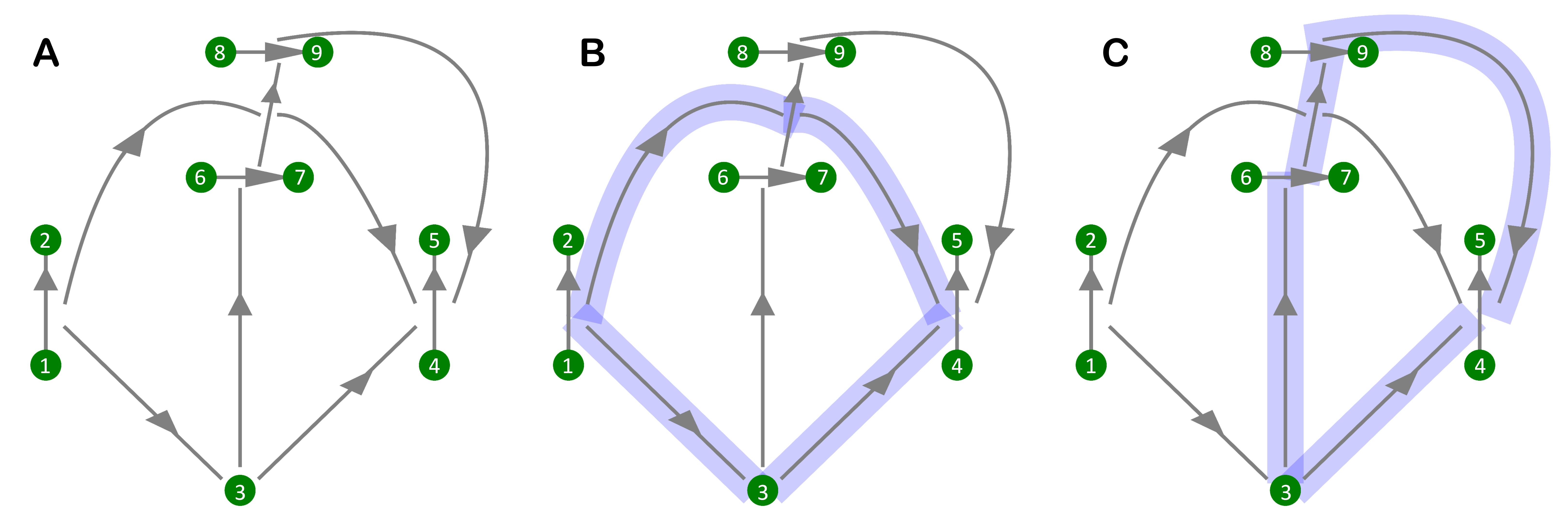
Figure 7: The subset $S$ of an IntComplex and its multilayer-homology. A: An IntComplex over $V=\{1,2,3,4,5,6,7,8,9\}$. The blue loops in B and C corresponds to the two multilayer-homology classes of $S$ respectively.

3.6 Join

Definition 12 (Join of Interactions).

Given two interactions $\sigma_{p}\in Int_{p}(V),\sigma_{q}\in Int_{q}(V)(1\leqslant p,q)$, define the join of $\sigma_{p}$ and $\sigma_{q}$ as the $(p+q)$-interaction $(\sigma_{p},\sigma_{q})\in Int_{p+q}(V).$

Clearly, join of interactions is a bilinear operation that does not satisfy associative law. Assume $\sigma_{p}=[v_{i_{1}}...v_{i_{p}},\{(l^{a}_{s},r^{a}_{s})\}_{s=1}^{p-1}]\in Int_{p}(V),\sigma_{q}=[v_{j_{1}}...v_{j_{q}},\{(l^{b}_{t},r^{b}_{t})\}_{t=1}^{q-1}]\in Int_{q}(V)$, then $(\sigma_{p},\sigma_{q})=[v_{i_{1}}...v_{i_{p}}v_{j_{1}}...v_{j_{q}},\{(l_{s}^{a},r_{s}^{a})\}_{s=1}^{p-1}\cup\{(l_{t}^{b}+p,r_{t}^{b}+p)\}_{t=1}^{q-1}\cup\{(1,p+q+1)\}]$.

Proposition 9 (Product rule).

$\forall\sigma_{p}\in Int_{p}(V),\sigma_{q}\in Int_{q}(V)$, $\partial(\sigma_{p},\sigma_{q})=(\partial(\sigma_{p}),\sigma_{q})+(-1)^{p}(\sigma_{p},\partial(\sigma_{q}))$.

Proof.

Assume $\sigma_{p}=[v_{i_{1}}...v_{i_{p}},\{(l^{a}_{s},r^{a}_{s})\}_{s=1}^{p-1}],\sigma_{q}=[v_{j_{1}}...v_{j_{q}},\{(l^{b}_{t},r^{b}_{t})\}_{t=1}^{q-1}]$.

$$\begin{split}\partial(\sigma_{p})&=\partial([v_{i_{1}}...v_{i_{p}},\{(l_{s}^{a},r_{s}^{a})\}_{s=1}^{p-1}])\\ &=\sum_{k=1}^{p}(-1)^{k+1}[v_{i_{1}}...v_{i_{k-1}}v_{i_{k+1}}...v_{i_{p}},N_{\sigma_{p}}^{k}].\\ (\partial(\sigma_{p}),\sigma_{q})&=\sum_{k=1}^{p}(-1)^{k+1}[v_{i_{1}}...v_{i_{k-1}}v_{i_{k+1}}...v_{i_{p}}v_{j_{1}}...v_{j_{q}},N_{\sigma_{p}}^{k}\cup\{(l_{t}^{b}+p,r_{t}^{b}+p)\}_{t=1}^{q-1}\cup\{(1,p+q)\}].\\ \partial(\sigma_{q})&=\partial([v_{j_{1}}...v_{j_{q}},\{(l_{t}^{b},r_{t}^{b})\}_{t=1}^{q-1}])\\ &=\sum_{k=1}^{q}(-1)^{k+1}[v_{j_{1}}...v_{j_{k-1}}v_{j_{k+1}}...v_{j_{q}},N_{\sigma_{q}}^{k}]\\ (-1)^{p}(\sigma_{p},\partial(\sigma_{q}))&=\sum_{k=1}^{q}(-1)^{p+k}[v_{i_{1}}...v_{i_{p}}v_{j_{1}}...v_{j_{k_{1}}}v_{j_{k+1}}...v_{j_{q}},\{(l_{s}^{a},r_{s}^{a})\}_{s=1}^{p-1}\cup(N_{\sigma_{q}}^{k}+p)\cup\{(1,p+q)\}]\end{split}$$

Here $N_{\sigma_{q}}^{k}+p=\{(a+p,b+p)|(a,b)\in N_{\sigma_{q}}^{k}\}$

$$\begin{split}&\quad(\partial(\sigma_{p}),\sigma_{q})+(-1)^{p}(\sigma_{p},\partial(\sigma_{q}))\\ &=\sum_{k=1}^{p}(-1)^{k+1}[v_{i_{1}}...v_{i_{k-1}}v_{i_{k+1}}...v_{i_{p}}v_{j_{1}}...v_{j_{q}},N_{\sigma_{p}}^{k}\cup\{(l_{t}^{b}+p,r_{t}^{b}+p)\}_{t=1}^{q-1}\cup\{(1,p+q)\}]\\ &+\sum_{k=1}^{q}(-1)^{p+k}[v_{i_{1}}...v_{i_{p}}v_{j_{1}}...v_{j_{k_{1}}}v_{j_{k+1}}...v_{j_{q}},\{(l_{s}^{a},r_{s}^{a})\}_{s=1}^{p-1}\cup(N_{\sigma_{q}}^{k}+p)\cup\{(1,p+q)\}\cup\{(1,p+q)\}]\\ &=\sum_{k=1}^{p}(-1)^{k+1}[v_{i_{1}}...v_{i_{k-1}}v_{i_{k+1}}...v_{i_{p}}v_{j_{1}}...v_{j_{q}},N_{\sigma_{p}}^{k}\cup\{(l_{t}^{b}+p,r_{t}^{b}+p)\}_{t=1}^{q-1}\cup\{(1,p+q)\}]\\ &+\sum_{k=p+1}^{p+q}(-1)^{k}[v_{i_{1}}...v_{i_{p}}v_{j_{1}}...v_{j_{k_{1}}}v_{j_{k+1}}...v_{j_{q}},\{(l_{s}^{a},r_{s}^{a})\}_{s=1}^{p-1}\cup(N_{\sigma_{q}}^{k-p}+p)\cup\{(1,p+q)\}]\\ &=\sum_{k=1}^{p}(-1)^{k+1}[v_{i_{1}}...v_{i_{k-1}}v_{i_{k+1}}...v_{i_{p}}v_{j_{1}}...v_{j_{q}},N_{(\sigma_{p},\sigma_{q})}^{k}]\\ &+\sum_{k=p+1}^{p+q}(-1)^{k+1}[v_{i_{1}}...v_{i_{p}}v_{j_{1}}...v_{j_{k-1}}v_{j_{j+1}}...v_{j_{q}},N_{(\sigma_{p},\sigma_{q})}^{k}]\\ &=\partial(\sigma_{p},\sigma_{q})\end{split}$$

∎

3.7 Interaction map

Definition 13 (Interaction map).

Given two IntComplex $\mathcal{I},\mathcal{I}^{\prime}$ over $V$ and $V^{\prime}$ respectively, assume $f:V\rightarrow V^{\prime}$ is a vertex map. For an interaction $\sigma=[v_{1}...v_{k},\{(l_{i},r_{i})\}_{i=1}^{k-1}]\in\mathcal{I}$, let $f(\sigma)=[f(v_{1})...f(v_{k}),\{(l_{i},r_{i})\}_{i=1}^{k-1}]$, if $f(\sigma)\in\mathcal{I}^{\prime}$ for $\forall\sigma\in\mathcal{I}$, $f$ is called an interaction map from $\mathcal{I}$ to $\mathcal{I}^{\prime}$.

The interaction map $f:\mathcal{I}\rightarrow\mathcal{I}^{\prime}$ sends an $n$-interaction of $\mathcal{I}$ to an $n$-interaction of $\mathcal{I}^{\prime}$.

Proposition 10.

Given an interaction map $f:\mathcal{I}\rightarrow\mathcal{I}^{\prime}$, $\forall\sigma=(\sigma_{p},\sigma_{q})\in\mathcal{I}$ $f(\sigma)=f(\sigma_{p},\sigma_{q})=(f(\sigma_{p}),f(\sigma_{q}))$

Proof.

Assume $\sigma_{p}=[v_{i_{1}}...v_{i_{p}},\{(l^{a}_{s},r^{a}_{s})\}_{s=1}^{p-1}],\sigma_{q}=[v_{j_{1}}...v_{j_{q}},\{(l^{b}_{t},r^{b}_{t})\}_{t=1}^{q-1}]$, we have

$(\sigma_{p},\sigma_{q})=[v_{i_{1}}...v_{i_{p}}v_{j_{1}}...v_{j_{q}},\{(l_{s}^{a},r_{s}^{a})\}_{s=1}^{p-1}\cup\{(l_{t}^{b}+p,r_{t}^{b}+p)\}_{t=1}^{q-1}\cup\{(1,p+q+1)\}]$.

$$\begin{split}f(\sigma_{p},\sigma_{q})&=[f(v_{i_{1}})...f(v_{i_{p}})f(v_{j_{1}})...f(v_{j_{q}}),\{(l_{s}^{a},r_{s}^{a})\}_{s=1}^{p-1}\cup\{(l_{t}^{b}+p,r_{t}^{b}+p)\}_{t=1}^{q-1}\cup\{(1,p+q+1)\}]\\ &=([f(v_{i_{1}})...f(v_{i_{p}}),\{(l_{s}^{a},r_{s}^{a})\}_{s=1}^{p-1}],[f(v_{j_{1}})...f(v_{j_{q}}),\{(l_{t}^{b},r_{t}^{b})\}_{t=1}^{q-1}])\\ &=(f(\sigma_{p}),f(\sigma_{q}))\end{split}$$

∎

Proposition 11.

Given an interaction map $f:\mathcal{I}\rightarrow\mathcal{I}^{\prime}$, $f\partial=\partial f$.

Proof.

$\forall\sigma_{1}\in\mathcal{I}_{1},$ $f(\partial(\sigma_{1}))=0=\partial(f(\sigma_{1}))$. Assume $f(\partial(\sigma_{p}))=\partial(f(\sigma_{p}))$ for $\forall\sigma_{p}\in\mathcal{I}_{p},\forall p<n$. Now we consider $n$-interactions, $\forall\sigma_{n}\in\mathcal{I}_{n}$, $\exists\sigma_{p}\in\mathcal{I}_{p},\sigma_{q}\in\mathcal{I}_{q},p,q<n$ such that $\sigma_{n}=(\sigma_{p},\sigma_{q})$.

$$\begin{split}\partial(f(\sigma_{n}))&=\partial(f(\sigma_{p},\sigma_{q}))\\ &=\partial(f(\sigma_{p}),f(\sigma_{q}))\\ &=(\partial(f(\sigma_{p}),f(\sigma_{q})+(-1)^{p}(f(\sigma_{p}),\partial(f(\sigma_{q})))\\ &=(f(\partial(\sigma_{p})),f(\sigma_{q}))+(-1)^{p}(f(\sigma_{p}),f(\partial(\sigma_{q})))~~(by~induction)\\ &=f(\partial(\sigma_{p}),\sigma_{q})+(-1)^{p}f(\sigma_{p},\partial(\sigma_{q}))\\ &=f(\partial(\sigma_{p},\sigma_{q}))\\ &=f(\partial(\sigma_{n}))\end{split}$$ (1)

Hence the result follows. ∎

Consequently, $f:\mathcal{I}\rightarrow\mathcal{I}^{\prime}$ induces a chain map $f_{*}:(\Lambda_{*}(\mathcal{I}),\partial_{*})\rightarrow(\Lambda_{*}(\mathcal{I}^{\prime}),\partial_{*})$.

Proposition 12.

Given an interaction map $f:\mathcal{I}\rightarrow\mathcal{I}^{\prime}$, the map $f_{*}|_{\Omega_{*}(\mathcal{I})}$ provides a chain map

$$f_{*}|_{\Omega_{*}(\mathcal{I})}:\Omega_{*}(\mathcal{I})\rightarrow\Omega_{*}(\mathcal{I}^{\prime})$$

consequently, a homomorphism of homology groups

$$f_{\#}:H_{*}(\mathcal{I})\rightarrow H_{*}(\mathcal{I}^{\prime})$$

Proof.

It suffices to prove that $f(\Omega_{p}(\mathcal{I}))\subset\Omega_{p}(\mathcal{I}^{\prime})$. Firstly we have $f(\mathcal{A}_{p}(\mathcal{I}))\subset\mathcal{A}_{p}(\mathcal{I}^{\prime})$. $\forall\sigma\in\Omega_{p}(\mathcal{I})$, we have $\sigma\in\mathcal{A}_{p}(\mathcal{I}),\partial(\sigma)\in\mathcal{A}_{p-1}(\mathcal{I})$, so $f(\sigma)\in\mathcal{A}_{p}(\mathcal{I}^{\prime})$, $\partial(f(\sigma))=f(\partial(\sigma))\in\mathcal{A}_{p-1}(\mathcal{I}^{\prime})$, which means $f(\sigma)\in\Omega_{p}(\mathcal{I}^{\prime})$. Hence $f(\Omega_{p}(\mathcal{I}))\subset\Omega_{p}(\mathcal{I}^{\prime})$. ∎

Proposition 13 (Functoriality of Homology).

Let $\mathcal{I},\mathcal{I}^{\prime},\mathcal{I}^{\prime\prime}$ be three IntComplexes.

1. Let $id_{\mathcal{I}}:\mathcal{I}\rightarrow\mathcal{I}$ be the identity interaction map. Then $({id_{\mathcal{I}}}_{\#})_{p}:H_{p}(\mathcal{I})\rightarrow H_{p}(\mathcal{I})$ is the identity linear map for each $p>0$.

2. Let $f:\mathcal{I}\rightarrow\mathcal{I}^{\prime}$, $g:\mathcal{I}^{\prime}\rightarrow\mathcal{I}^{\prime\prime}$ be interaction maps. Then $((gf)_{\#})_{p}=(g_{\#})_{p}(f_{\#})_{p}$ for each $p>0$.

Proof.

For the first claim: $\forall\sigma_{p}=[v_{1}...v_{p},\{(l_{i},r_{i})\}_{i=1}^{p-1}]\in\Omega_{p}(\mathcal{I})$,

$$\begin{split}(id_{\mathcal{I}_{*}})_{p}(\sigma_{p})&=[id_{\mathcal{I}}(v_{1})...id_{\mathcal{I}}(v_{p}),\{(l_{i},r_{i})\}_{i=1}^{p-1}]\\ &=[v_{1}...v_{p},\{(l_{i},r_{i})\}_{i=1}^{p-1}]\\ &=\sigma_{p}\end{split}$$

It follows that $(id_{\mathcal{I}_{*}})_{p}$ is the identity map on $\Omega_{p}(\mathcal{I})$, and thus $(id_{\mathcal{I}_{\#}})_{p}$ is the identity map on $H_{p}(\mathcal{I})$.

For the second claim: $\forall\sigma_{p}=[v_{1}...v_{p},\{(l_{i},r_{i})\}_{i=1}^{p-1}]\in\Omega_{p}(\mathcal{I})$,

$$\begin{split}((gf)_{*})_{p}(\sigma_{p})&=[gf(v_{1})...gf(v_{p}),\{(l_{i},r_{i})\}_{i=1}^{p-1}]\\ &=[g(f(v_{1}))...g(f(v_{p})),\{(l_{i},r_{i})\}_{i=1}^{p-1}]\\ &=(g_{*})_{p}([f(v_{1})...f(v_{p}),\{(l_{i},r_{i})\}_{i=1}^{p-1}])\\ &=(g_{*})_{p}(f_{*})_{p}([v_{1}...v_{p},\{(l_{i},r_{i})\}_{i=1}^{p-1}])\\ &=(g_{*})_{p}(f_{*})_{p}(\sigma_{p})\end{split}$$

The result follows. ∎

4 Persistent Homology of IntComplex

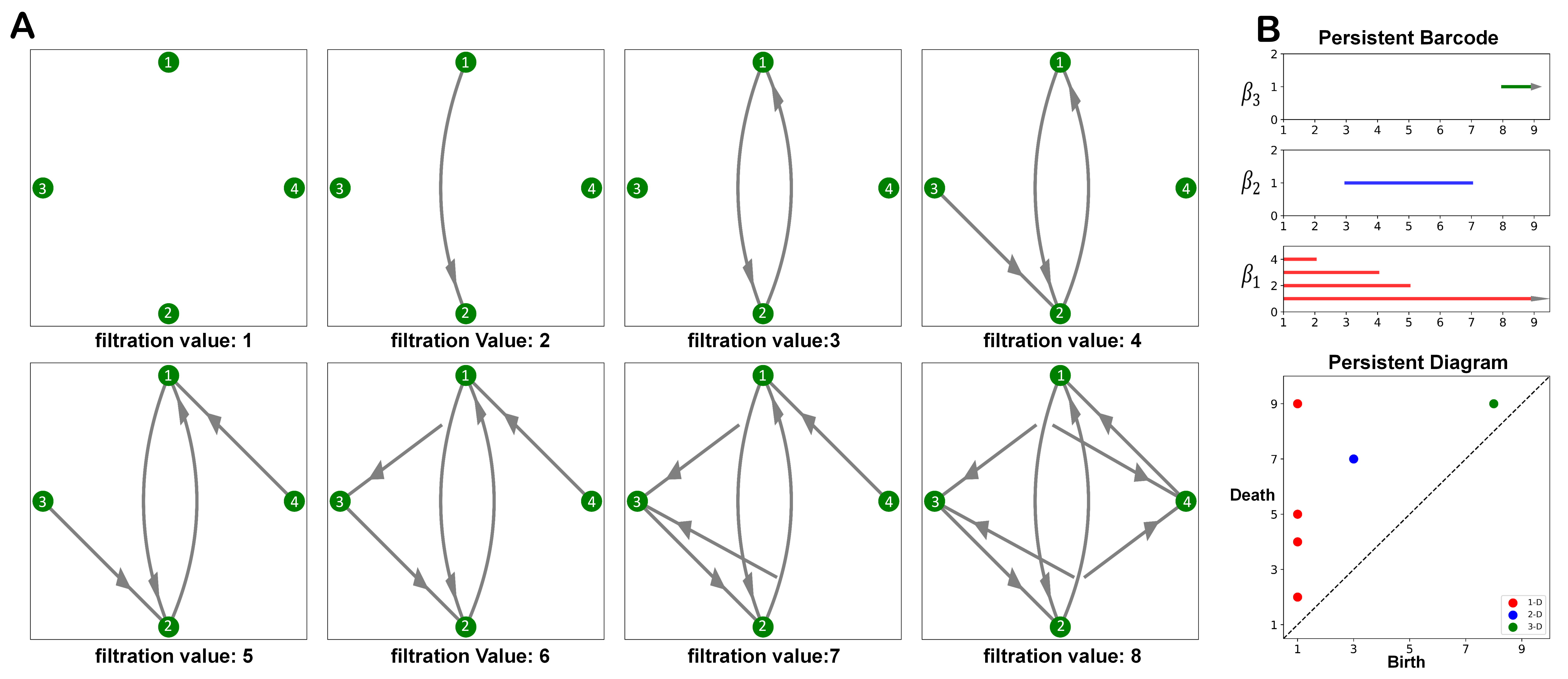
Figure 8: Illustration of the persistent homology of an IntComplex. A: the filtration of an IntComplex. B: the persistent barcode and peristent diagram representation of the persistent homology.

As a key theory of topological data analysis (TDA), persistent homology has been successfully applied to various fields. Here we give the persistent homology of IntComplex.

4.1 Persistent homology

Definition 14 (IntComplex filtration).

A filtration of the IntComplex $\mathcal{I}$ is a sequence of IntComplexes

$$\mathcal{I}(1)\subset\mathcal{I}(2)\subset...\subset\mathcal{I}(n)=\mathcal{I}$$

where $\mathcal{I}(p)$ is a subcomplex of $\mathcal{I}(p+1)$, they are connected by inclusion map $(1\leqslant p<n).$

The functoriality of homology enables us to obtain a persistent vector spaces from an IntComplex filtration, we give the definition as follows:

Definition 15 (Persistent homology of IntComplex).

Given an IntComplex filtration $\{\mathcal{I}(k)\xrightarrow{i_{k}}\mathcal{I}(k+1)\}_{0\leqslant k}$ of $\mathcal{I}$. Then for each $p>0$, the p-th persistent homology of the filtration is defined as the following persistent vector space:

$$H_{p}^{q}(\mathcal{I})=Im\{H_{p}(\mathcal{I}(k))\xrightarrow{(i_{k,k+q})_{\#}}H_{p}(\mathcal{I}(k+q))\}_{q>0,k>0}$$

Then define the p-th persistent diagram of the filtration $\mathcal{I}$ to be the persistent diagram of $H_{p}^{q}(\mathcal{I})$.

Definition 16 (Weighted InComplex).

A weighted IntComplex is a pair $(\mathcal{I},f)$ where $\mathcal{I}$ is an IntComplex $\mathcal{I}$ and $f$ is a function $f:\mathcal{I}\rightarrow R$, denoted by $\mathcal{I}^{f}$. let $\mathcal{I}(r)=\{\sigma|f(\sigma)\leqslant r\}$, then we get an IntComplex filtration $\{\mathcal{I}(r)\xrightarrow{i}\mathcal{I}(s)\}_{r<s}$. We denote the persistent homology and persistent diagram of this filtration by $H(\mathcal{I},f)$ and $\mathcal{D}(\mathcal{I}^{f})$ respectively.

Example 7.

Consider a weighted IntComplex $\mathcal{I}$ over $V=\{1,2,3,4\}$, $\mathcal{I}=\{[1,1]$, $[2,1]$, $[3,1]$, $[4,1]$, $[(1,2),2]$, $[(2,3),3]$, $[(3,2),4]$, $[(4,1),5]$, $[((1,2),3),6]$, $[((2,1),3),7]$, $[((1,2),4),8]$, $[((2,1),4),8]\}$ where $[\sigma,v]$ represents an interaction $\sigma$ with weight $v$, denoted by $w(\sigma)=v$. Let $\mathcal{I}(k)=\{\sigma|w(\sigma)\leqslant k\}$. Then we get a filtration of $\mathcal{I}$,

$$\mathcal{I}(1)\subset\mathcal{I}(2)\subset\mathcal{I}(3)\subset\mathcal{I}(4)\subset\mathcal{I}(5)\subset\mathcal{I}(6)\subset\mathcal{I}(7)\subset\mathcal{I}(8)$$

which is shown in Figure 8 A. The persistent homology is computed and represented by persistent barcode and persistent diagram as in Figure 8 B.

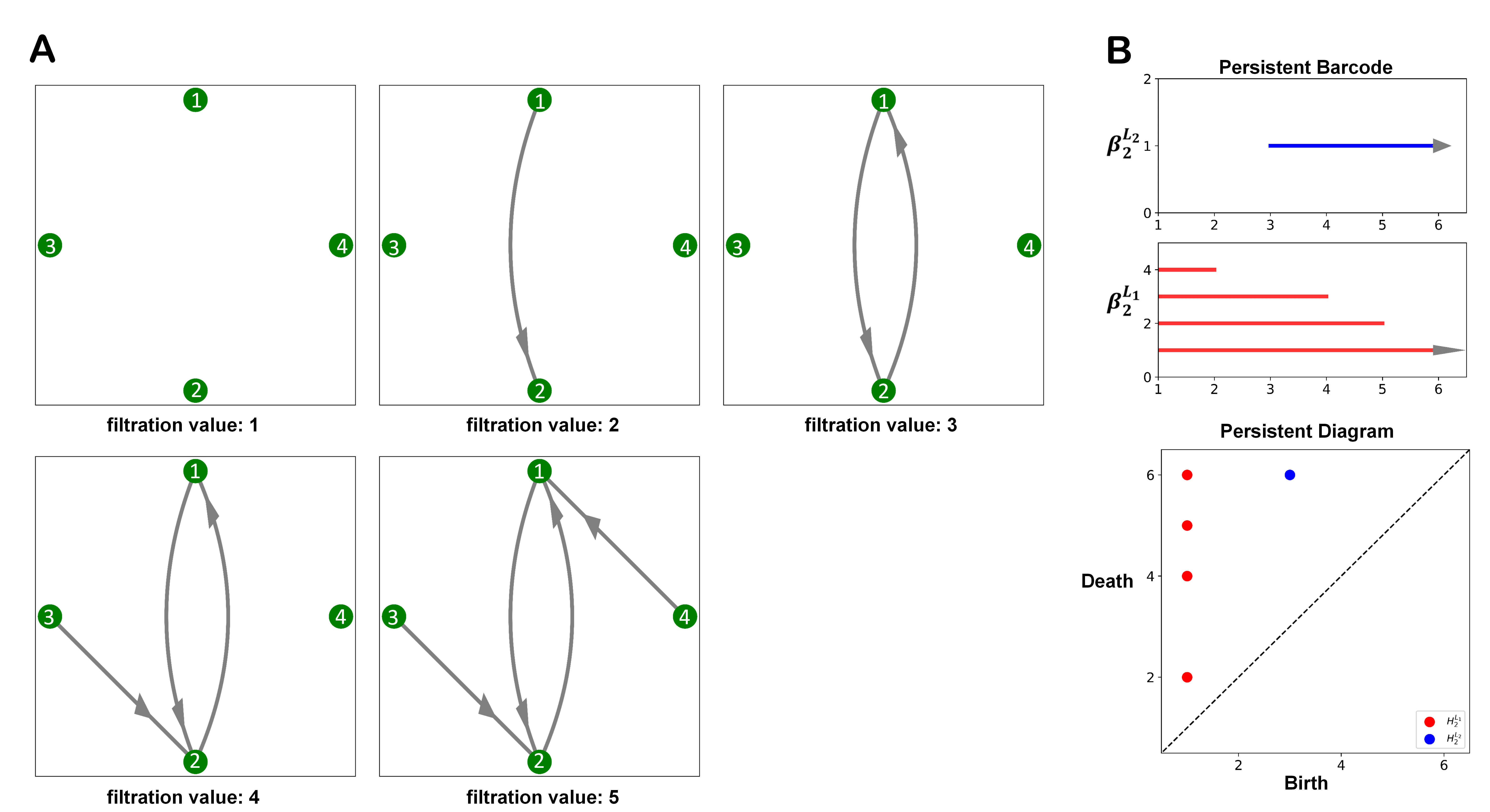
Figure 9: Illustration of the persistent $p$-layer-homology of an weighted IntComplex. A: the induced filtration for $p=2$. B: the persistent barcode and peristent diagram representation of the persistent 2-layer-homology.

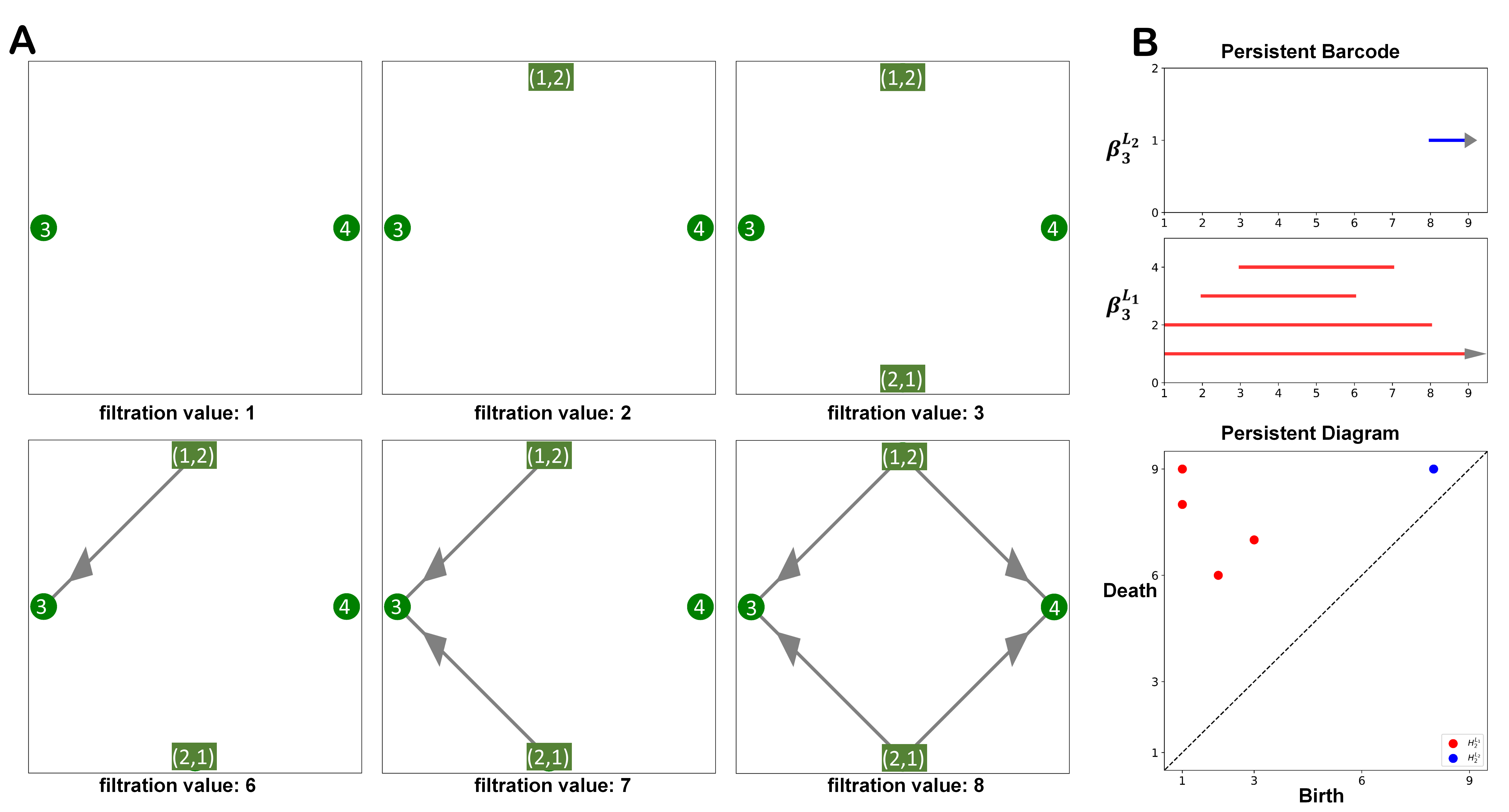
Figure 10: Illustration of the persistent $p$-layer-homology of an weighted IntComplex. A: the induced filtration for $p=3$. B: the persistent barcode and peristent diagram representation of the persistent 3-layer-homology.

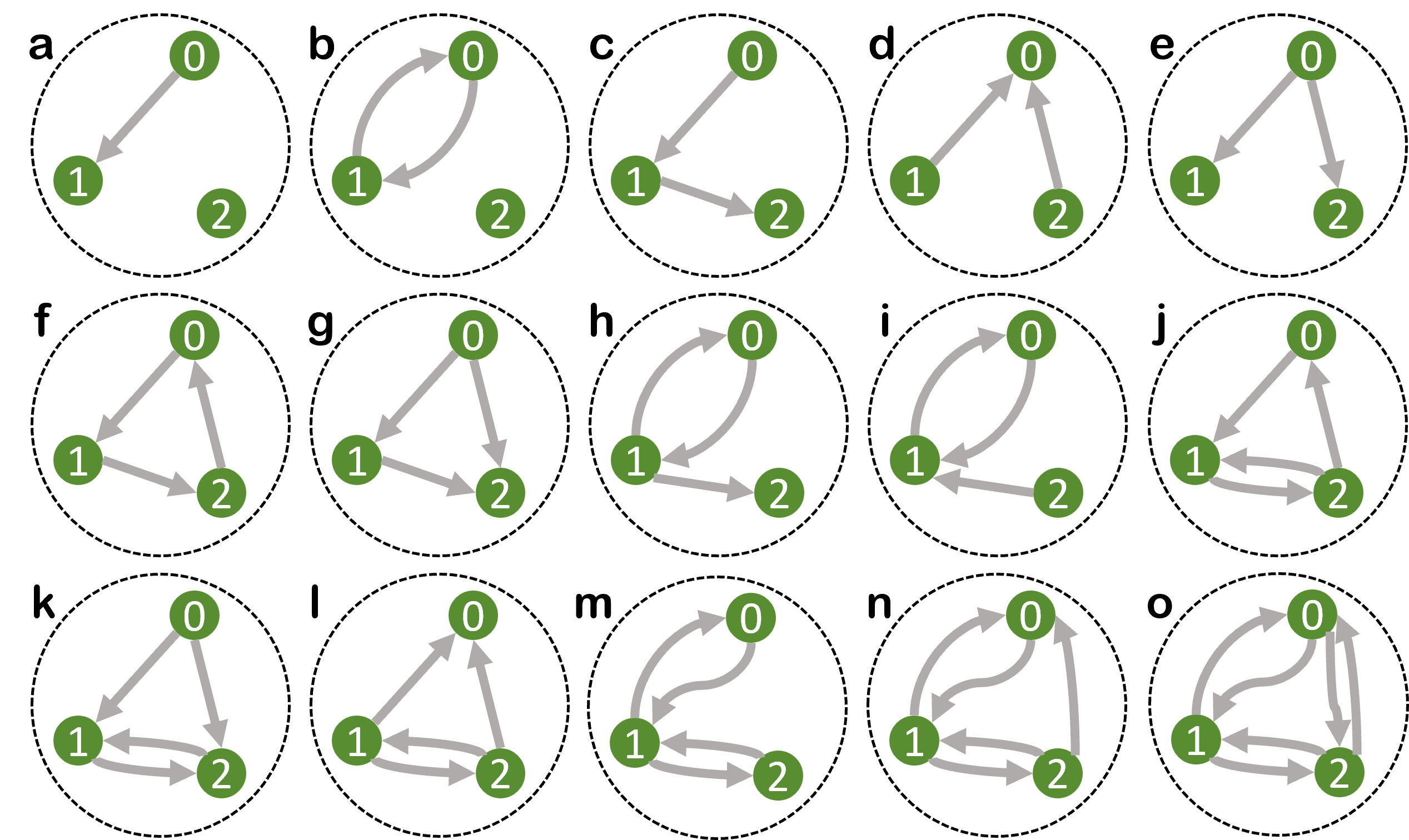
Figure 11: Fifteen types of digraphs with at least one arrow over three vertices.

4.2 Stability of persistent homology

The persistent diagram of an IntComplex filtration is a multi-set of pairs in which each pair $(b_{i},d_{i})$ represents a homology class that appears at filtration $b_{i}$ and disappears at filtration $d_{i}$. Note that $d_{i}$ can be $\infty$ and we define $|(+\infty)-(+\infty)|=|(-\infty)-(-\infty)|=0$. For any two pairs $p_{i}=(b_{i},d_{i}),p_{j}=(b_{j},d_{j})$, define $d^{\infty}(p_{i},p_{j})=\max\{|b_{i}-b_{j}|,|d_{i}-d_{j}|\}$ and $d^{\infty}(p_{i})=(d_{i}-b_{i})/2$.

Definition 17 (Partial matching).

A partial matching between multi-sets $A$ and $B$ is a collection of pairs $\psi=\{(\alpha,\beta)\in A\times B\}$ where $\alpha$ and $\beta$ can occur in at most one pair. If $(\alpha,\beta)\in\psi$, we say that $\alpha$ is matched with $\beta$, otherwise if $\alpha$ does not belong to any pair in $\psi$, we say $\alpha$ is unmatched.

Definition 18 ($\delta$-matching).

A partial matching $\psi$ between A and B is called a $\delta$-matching if

• $\forall(\alpha,\beta)\in\psi$, $d^{\infty}(\alpha,\beta)\leqslant\delta$

• if $\alpha\in A\cup B$ is unmatched, $d^{\infty}(\alpha)\leqslant\delta$

Definition 19 (Bottleneck distance).

The bottleneck distance between two multi-sets $A$ and $B$ is defined as

$$d_{B}(A,B)=\inf\{\delta|there~exists~a~\delta\text{-}matching~between~A~and~B\}$$

As with any category, a homomorphism of degree $\epsilon$ between two persistence modules $\mathbb{U}=\{U_{s}\xrightarrow{u_{s}^{t}}{U_{t}}\}$ and $\mathbb{V}=\{V_{s}\xrightarrow{v_{s}^{t}}V_{t}\}$ is a collection $\Phi$ of module morphisms $\phi_{t}:U_{t}\rightarrow V_{t+\epsilon}$ such that $\phi_{t}u_{s}^{t}=v_{s+\epsilon}^{t+\epsilon}\phi_{s}$ for all $s\leqslant t$. Let ${\rm Hom}^{\epsilon}(\mathbb{U},\mathbb{V})$ be the collection of all homomorphism of degree $\epsilon$ from $\mathbb{U}$ to $\mathbb{V}$.

Definition 20 ($\epsilon$-interleaved).

Two persistence modules $\mathbb{U}$ and $\mathbb{V}$ are called $\epsilon$-interleaved if there are maps

$$\Phi\in{\rm Hom}^{\epsilon}(\mathbb{U},\mathbb{V}),\Psi\in{\rm Hom}^{\epsilon}(\mathbb{V},\mathbb{U})$$

such that

$$\Phi\Psi=1_{\mathbb{V}}^{2\epsilon},\Psi\Phi=1_{\mathbb{U}}^{2\epsilon}$$

Definition 21 (Interleaving distance).

The interleaving distance between two persistence modules $\mathbb{U}$ and $\mathbb{V}$ is defined as

$$d_{I}(\mathbb{U},\mathbb{V})=\inf\{\epsilon|\mathbb{U}~and~\mathbb{V}~are~\epsilon\text{-}interleaved\}$$

Let $f,g$ be two real-valued functions defined on an finite IntComplex $\mathcal{I}$, $||f-g||_{\infty}=\sup\limits_{\sigma\in\mathcal{I}}{|f(\sigma)-g(\sigma)|}$, $\mathcal{D}(\mathcal{I}^{f})$ and $\mathcal{D}(\mathcal{I}^{g})$ be the persistence diagrams of $\mathcal{I}$ induced by $f$ and $g$ respectively. We have the following result:

Theorem 2 (Stability of persistent homology).

$$d_{B}(\mathcal{D}(\mathcal{I}^{f}),\mathcal{D}(\mathcal{I}^{g}))\leqslant||f-g||_{\infty}$$

.

Proof.

From the algebraic stability, we have

$$d_{I}(H(\mathcal{I},f),H(\mathcal{I},g))=d_{I}(\mathcal{D}(\mathcal{I}^{f}),\mathcal{D}(\mathcal{I}^{g}))$$

Considering the category $\mathcal{C}$ of filtered IntComplex in which objects are filtered IntComplexs and morphisms are the interaction maps between them. $\mathcal{I}^{f},\mathcal{I}^{g}\in\mathcal{C}$. Let $\epsilon=||f-g||_{\infty}$, we prove that $\mathcal{I}^{f}$ and $\mathcal{I}^{g}$ are $\epsilon$-interleaved in $\mathcal{C}$.

We have the inclusions of IntComplexs $\mathcal{I}^{f}_{a}\hookrightarrow\mathcal{I}^{f}_{a+\epsilon}$, $\mathcal{I}^{g}_{a}\hookrightarrow\mathcal{I}^{g}_{a+\epsilon}$. Note that $\mathcal{I}^{f}_{a}$ and $\mathcal{I}^{g}_{a}$ are subcomplexes of $\mathcal{I}^{g}_{a+\epsilon}$ and $\mathcal{I}^{f}_{a+\epsilon}$ respectively. So we have the homomorphisms

$$\Phi:\mathcal{I}^{f}_{\star}\hookrightarrow\mathcal{I}^{g}_{\star+\epsilon},\Psi:\mathcal{I}^{g}_{\star}\hookrightarrow\mathcal{I}^{f}_{\star+\epsilon}$$

All the morphisms are inclusions, so we have

$$\Psi\Phi=1_{\mathcal{I}^{f}_{\star}}^{2\epsilon},\Phi\Psi=1_{\mathcal{I}^{g}_{\star}}^{2\epsilon}$$

Consequently, $\mathcal{I}^{f}$ and $\mathcal{I}^{g}$ are $\epsilon$-interleaved, which means

$$d_{I}(\mathcal{I}^{f},\mathcal{I}^{g})\leqslant\epsilon$$

by the functoriality of IntComplex homology, we have

$$d_{I}(H(\mathcal{I}^{f}),H(\mathcal{I}^{g}))\leqslant d_{I}(\mathcal{I}^{f},\mathcal{I}^{g})\leqslant\epsilon$$

So

$$d_{I}(\mathcal{D}(\mathcal{I}^{f})\mathcal{D}(\mathcal{I}^{g}))\leqslant\epsilon$$

from the result in, we have

$$d_{B}(\mathcal{D}(\mathcal{I}^{f}),\mathcal{D}(\mathcal{I}^{g})\leqslant||f-g||_{\infty}$$

∎

Definition 22 (Persistent $p$-layer-homology of weighted IntComplex).

Given a weighted IntComplex $\hat{\mathcal{I}}=(\mathcal{I},f)$, consider $G_{p}^{\mathcal{I}}$, we get a weighted IntComplex $\mathcal{I}^{\prime}=(G_{p}^{\mathcal{I}},f|_{G_{p}^{\mathcal{I}}})$. Then we can get a IntComplex filtration from $\mathcal{I}^{\prime}$ by definition 16, the persistent homology of this filtration is defined as the persistent $p$-layer homology of $\hat{\mathcal{I}}$.

Example 8.

For the weighted IntComplex $\mathcal{I}$ in Example 7, we consider the persistent $p$-layer homology, the induced filtration for $p=2$ is shown in Figure 9 A. And the associated persistent $2$-layer homology is illustrated by persistent barcode and persistent diagram in Figure 9 B.

The induced filtration for $p=3$ is shown in Figure 10 A. And the associated persistent $3$-layer homology is illustrated by persistent barcode and persistent diagram in Figure 10 B.

Note that for $p=3$, the 1-interaction set is $\{3,4,(1,2),(2,1)\}$, 2-interaction set is all the 3-interactions of $\mathcal{I}$.

5 Experimental analysis

In this section, we give experimental test to show the importance of high-order interactions for network analysis.

Considering the digraphs without self-loops over three vertices. There are 15 types of such digraphs with at least one arrow up to graph isomorphism, which is shown in Figure 11.

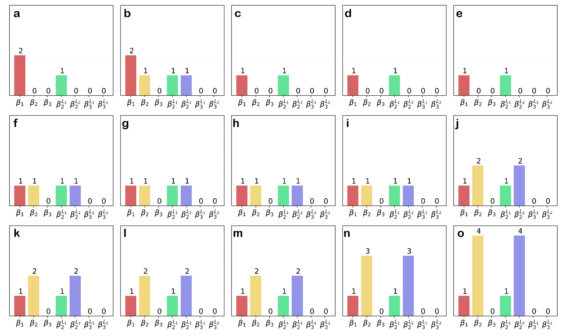
Figure 12: Homology, 2-layer homology and 3-layer homology of the 15 digraphs in Figure 11. It can be seen that some non-isomorphic digraphs share the same homology information.

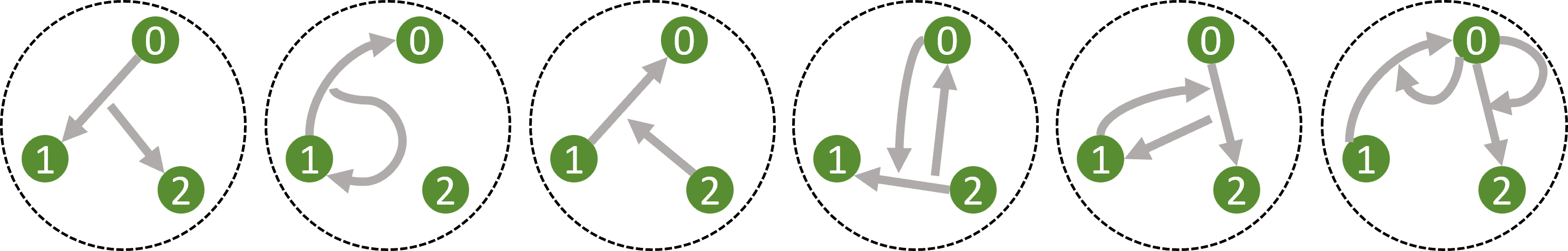
Figure 13: The 3-interactions that are added to the 15 digraphs in Figure 12.

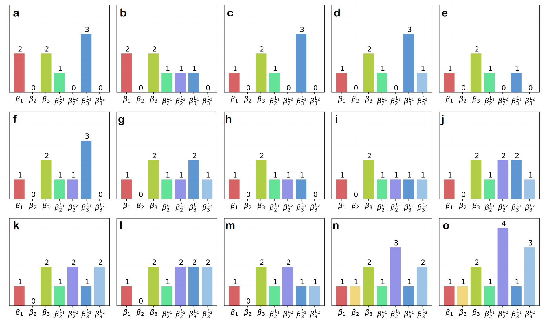
Figure 14: Homology, 2-layer homology and 3-layer homology of the IntComplexes derived from the 15 digraphs by adding the 3-interactions in Figure 13. It can be seen that the homology information can clearly differentiate all 15 IntComplexes.

Among these digraphs, there is one digraph with one arrow (a), four digraphs with two arrows (b,c,d,e), four digraphs with three arrows (f,g,h,i), four digraphs with four arrows (j,k,l,m), one digraph with five arrows (n) and one digraph with six arrows (o).

Each digraph $G=(V,E)$ can be seen as an IntComplex $\mathcal{I}$ where $\mathcal{I}_{0}=V,\mathcal{I}_{1}=E$ and $\mathcal{I}_{p}=\emptyset(p>1)$. We compute the homology, 2-layer homology and 3-layer homology of these 15 digraphs. The results are shown in Figure 12. It can be seen that the four digraphs with three arrows (f,g,h,i) have the same homology information, the four digraphs with four arrows (j,k,l,m) have the same homology information, and three digraphs (c,d,e) with two arrows have the same homology information, which means the homology information cannot differentiate them.

As IntComplexes, these digraphs only have 1-interaction of independent identities and 2-interaction of pair-wise interactions. We add the following 3-interactions into all 15 IntComplexes to get 15 new IntComplexes with high-order interactions: ((0,1),2), ((1,0),1), (2,(1,0)), (0,(2,1)), ((2,1),0), (1,(0,2)), ((0,2),1), (0,(1,0)), (0,(0,2)). Figure 13 shows all these 3-interactions.

Then, we compute the homology, 2-layer homology and 3-layer homology of the new IntComplexes, the results are shown in Figure 14.

It can be seen that there are no two IntComplexes have the same homology information for all 15 IntComplexes. In a summary, before adding the 3-interactions, the fifteen digraphs cannot be differentiated by the homology information, while after adding some 3-interactions, all 15 digraphs can be clearly differentiated by the homology information.

6 Conclusion

In the work, we present IntComplex as a novel model for high-order interactions that existing graph, simplicial complex, and hypergraph models cannot represent. We introduce the homology theory, including the standard homology for adjacent order interactions, layer-homology for a specific order interactions and multi-layer homology for interactions across several orders, to give quantitative characterization of the IntComplex, enabling a detailed dissection of the topological structure of high-order interactions. Further, we introduce the persistent homology by considering the filtration process and give the stability result to ensure its robustness. IntComplex provides a foundational framework for analyzing the topological properties of high-order interactions, offering significant potential for advancing complex network analysis.

References

- [1] Narsingh Deo. Graph theory with applications to engineering and computer science. Courier Dover Publications, 2017.
- [2] Jonathan L Gross, Jay Yellen, and Mark Anderson. Graph theory and its applications. Chapman and Hall/CRC, 2018.
- [3] Antonio Ortega, Pascal Frossard, Jelena Kovačević, José MF Moura, and Pierre Vandergheynst. Graph signal processing: Overview, challenges, and applications. Proceedings of the IEEE, 106(5):808–828, 2018.
- [4] Wei Wang, Quan-Hui Liu, Junhao Liang, Yanqing Hu, and Tao Zhou. Coevolution spreading in complex networks. Physics Reports, 820:1–51, 2019.
- [5] Renaud Lambiotte, Martin Rosvall, and Ingo Scholtes. From networks to optimal higher-order models of complex systems. Nature physics, 15(4):313–320, 2019.
- [6] Federico Battiston, Giulia Cencetti, Iacopo Iacopini, Vito Latora, Maxime Lucas, Alice Patania, Jean-Gabriel Young, and Giovanni Petri. Networks beyond pairwise interactions: Structure and dynamics. Physics Reports, 874:1–92, 2020.
- [7] Leo Torres, Ann S Blevins, Danielle Bassett, and Tina Eliassi-Rad. The why, how, and when of representations for complex systems. SIAM Review, 63(3):435–485, 2021.
- [8] Federico Battiston, Enrico Amico, Alain Barrat, Ginestra Bianconi, Guilherme Ferraz de Arruda, Benedetta Franceschiello, Iacopo Iacopini, Sonia Kéfi, Vito Latora, Yamir Moreno, et al. The physics of higher-order interactions in complex systems. Nature Physics, 17(10):1093–1098, 2021.
- [9] Per Sebastian Skardal and Alex Arenas. Abrupt desynchronization and extensive multistability in globally coupled oscillator simplexes. Physical review letters, 122(24):248301, 2019.
- [10] Iacopo Iacopini, Giovanni Petri, Alain Barrat, and Vito Latora. Simplicial models of social contagion. Nature communications, 10(1):2485, 2019.
- [11] Leonie Neuhäuser, Andrew Mellor, and Renaud Lambiotte. Multibody interactions and nonlinear consensus dynamics on networked systems. Physical Review E, 101(3):032310, 2020.
- [12] Unai Alvarez-Rodriguez, Federico Battiston, Guilherme Ferraz de Arruda, Yamir Moreno, Matjaž Perc, and Vito Latora. Evolutionary dynamics of higher-order interactions in social networks. Nature Human Behaviour, 5(5):586–595, 2021.
- [13] James R Munkres. Elements of algebraic topology. CRC press, 2018.
- [14] Claude Berge. Hypergraphs: combinatorics of finite sets, volume 45. Elsevier, 1984.
- [15] Kelin Xia and Guo-Wei Wei. Persistent homology analysis of protein structure, flexibility, and folding. International journal for numerical methods in biomedical engineering, 30(8):814–844, 2014.
- [16] Zixuan Cang, Lin Mu, and Guo-Wei Wei. Representability of algebraic topology for biomolecules in machine learning based scoring and virtual screening. PLoS computational biology, 14(1):e1005929, 2018.
- [17] Xiang Liu, Xiangjun Wang, Jie Wu, and Kelin Xia. Hypergraph-based persistent cohomology (hpc) for molecular representations in drug design. Briefings in Bioinformatics, 22(5):bbaa411, 2021.
- [18] Xiang Liu, Huitao Feng, Jie Wu, and Kelin Xia. Dowker complex based machine learning (dcml) models for protein-ligand binding affinity prediction. PLoS Computational Biology, 18(4):e1009943, 2022.
- [19] Yasuaki Hiraoka, Takenobu Nakamura, Akihiko Hirata, Emerson G Escolar, Kaname Matsue, and Yasumasa Nishiura. Hierarchical structures of amorphous solids characterized by persistent homology. Proceedings of the National Academy of Sciences, 113(26):7035–7040, 2016.
- [20] Yongjin Lee, Senja D Barthel, Paweł Dłotko, S Mohamad Moosavi, Kathryn Hess, and Berend Smit. Quantifying similarity of pore-geometry in nanoporous materials. Nature communications, 8(1):1–8, 2017.
- [21] Mohammad Saadatfar, Hiroshi Takeuchi, Vanessa Robins, Nicolas Francois, and Yasuaki Hiraoka. Pore configuration landscape of granular crystallization. Nature communications, 8(1):15082, 2017.
- [22] D Vijay Anand, Qiang Xu, JunJie Wee, Kelin Xia, and Tze Chien Sum. Topological feature engineering for machine learning based halide perovskite materials design. npj Computational Materials, 8(1):203, 2022.
- [23] Kai Wang, Masumichi Saito, Brygida C Bisikirska, Mariano J Alvarez, Wei Keat Lim, Presha Rajbhandari, Qiong Shen, Ilya Nemenman, Katia Basso, Adam A Margolin, et al. Genome-wide identification of post-translational modulators of transcription factor activity in human b cells. Nature biotechnology, 27(9):829–837, 2009.
- [24] Dror Y Kenett, Xuqing Huang, Irena Vodenska, Shlomo Havlin, and H Eugene Stanley. Partial correlation analysis: Applications for financial markets. Quantitative Finance, 15(4):569–578, 2015.
- [25] Juan Zhao, Yiwei Zhou, Xiujun Zhang, and Luonan Chen. Part mutual information for quantifying direct associations in networks. Proceedings of the National Academy of Sciences, 113(18):5130–5135, 2016.
- [26] Anthony Baptista, Marta Niedostatek, Jun Yamamoto, Ben MacArthur, Jurgen Kurths, Ruben Sanchez Garcia, and Ginestra Bianconi. Mining higher-order triadic interactions. arXiv preprint arXiv:2404.14997, 2024.